Performance Analysis of Metaheuristic Optimization Algorithms in Estimating the Interfacial Heat Transfer Coefficient on Directional Solidification

Abstract

In this paper is proposed an evaluation of ten metaheuristic optimization algorithms applied on the inverse optimization of the Interfacial Heat Transfer Coefficient (IHTC) coupled on the solidification phenomenon. It was considered an upward directional solidification system for Al-7wt.% Si alloy and, for IHTC model, a exponential time function. All thermophysical properties of the alloy were considered constant. Scheil Rule was used as segregation model ahead phase-transformation interface. Optimization results from Markov Chain Monte Carlo method (MCMC) were considered as reference. Based on average, quantiles 95% and 5%, kurtosis, average iterations and absolute errors of the metaheuristic methods, in relation to MCMC results, the Flower Pollination Algorithm (FPA) and Moth-Flame Optimization (MFO) presented the most appropriate results, outperforming the other methods in this particular phenomenon, based on these metrics. The regions with the most probable values for parameters in IHTC time function were also determined.

Keywords— Casting process optimization, Stochastic method application, Nature-inspired algorithms, A444.0 alloy, Permanent mold casting

1 Introduction

Many problems in science deal with parameters uncertainty. As a result, predictions of nature’s behavior may lose accuracy and scientific conclusions may be compromised. To overcome this problem several algorithms, called optimization methods, have been proposed. These computational strategies play an important role: parameter estimation using numerical routines derived from differential operators, bayesian methodologies or even nature observations techniques. In the last case, studies involving the so-called Nature-Inspired Optimization Algorithms (NIOA) and Metaheuristic Optimization Algorithms (MOA) are usual. These methods are based on a local and global random search and use weighting mechanisms adapted from the behavior of, for example, living beings, celestial bodies and natural phenomena. In this group of algorithms, it is worth pointing out widely used ones to predict parameters, such as Simulated Annealing [27], Ant Colony Optimization [17, 30], Cuckoo Search [64, 13], Wind Driven Algorithm [5, 2], Tree-Seed Algorithm [26, 7], Water Wave Optimization [67, 45], Tree-Growth Algorithm [12], Sailfish Optimizer [44] and Manta Ray Foraging Optimization [66]. Due to easy of implementation, exploration and exploitation search, convergence speed and operational versatility, these algorithms have become popular in parameter estimation in several applications, such as crack propagation [11], design of heat exchangers [15], photovoltaic systems [53], power control of wind turbine [6], strategic aircraft deconfliction [14], optimal power flow problems [3], hybrid renewable systems [41] and others.

By No Free Lunch (NFL) theorems [63, 24], originally established for search in [56] and for optimization in [57], it is known that no optimization algorithm is better than others over all possible functions and real-world problems. However, ss reminded by [31], despite of some incorrect ideas about NFL, the original statement does not ignore the fact that there is some algorithm $A$ that can outperform $B$, once $A$ could be specialized to the set of problems analyzed in the case. NFL encourages researchers to identify this specialization [61]. One can do that by creating a tailored-hand algorithm to the problem to achieve better than random performance or identifying among all developed algorithms one that is already specialized to some or a particular problem subset. So, it is necessary to analyze case-by-case the performance of metaheuristic methods to define, in a restrictive way to the physical model, which method outperforms others in terms of parameter estimation, processing time, operational cost and other quantitative and qualitative requirements.

In this context, there has been little information available about the effectiveness of optimization metaheuristic methods in specific applications of Mechanical Engineering and Metallurgy. Even though in many papers the optimization of test functions is approached [58, 19], there is also great utility in verifying the numerical performance of the optimization methods in more complex, real-world problems. One of these is the transient heat and mass transfer coupled with phase transformation, that is, the phenomenon of solidification on permanent metallic mold castings. In this process, the Interfacial Heat Transfer Coefficient (IHTC) represents one of the most important thermal coefficients since it predominantly controls the heat transfer of the metallic system, then directly influencing several thermal parameters. These can be explicitly related to the physical [42, 43] and mechanical [48, 8] metallurgy of the ingot. Although its relevance, this coefficient is of difficult estimation since it is not easy to measure experimentally and comes from a numerical ill-posed problem. In this way, it is necessary to use an optimization method that, from the experimental data, can infer this parameter from an inverse approach.

So, in this paper, ten optimization methods will be analyzed in order to determine which of them, in a solidification problem, returns the best temperature prediction, which are: Particle Swarm Optimization [25], Differential Evolution [50], Bat Algorithm [59], Flower Pollination Algorithm [60], Grey Wolf Optimizer [36], Moth-Flame Optimization [32], Sine Cosine Algorithm [34], Whale Optimization Algorithm [35], Dragonfly Algorithm [33] and Harris Hawks Optimization [22]. These methods were chosen based on their scientific relevance and applicability, once these methods have already been applied by several researchers in the most varied areas of science and their performances are notoriously recognized.

Markov Chain Monte Carlo (MCMC) method will be used in order to determine the statistical consistency of the results provided by the optimization algorithms under study. This method is widely used for estimations in materials and thermal science, such as thermal diffusivity of metals [20], heat flux [29], heat transfer coefficient [52] and metallic fatigue [4].

Therefore, the main contribution of this paper is a performance analysis of various metaheuristic algorithms on the inverse optimization of the IHTC in directional solidification. Results obtained via Markov Chain Monte Carlo will be considered, in order to determine, given the physical phenomenon, which method stands for the most appropriated for inference.

An aluminum-based alloy was the material chosen to be analyzed. This type of alloy has a notorious importance, since, in an effort to improve vehicle fuel efficiency by lower consumption, lightweight aluminum alloys have been replacing other materials for use in automotive integrated systems and components [23] such as engine blocks and cylinder heads [51] and also on aerospace and marine applications [28]. Among aluminum-based alloys, the aluminum-silicon (Al-Si) system has considerable prestige. Al-Si alloys are widely used in the automotive industry, especially on engines [9], due to their attractive strength to weight ratio as well as superior casting characteristics [40]. Regarding the production volume, Al-Si alloys account for 80 to 90% of the aluminum castings produced commercially [47]. Based on this author, there is an optimum range of silicon content, depending on the casting process: 5 to 7wt.% Si for slow cooling-rate processes, such as casting in plaster, investment, and sand molds; 7 to 9wt. % Si for permanent molds; and 8 to 12wt. % Si for die casting.

Therefore, given the industrial and academic relevance of this non-ferrous system and its usage ranges, this paper chose Al-7wt.% Si (also registered by the Aluminum Association (AA) under the number A444.0) as the study alloy. This alloy, especially on permanent mold casting, exhibit excellent proprieties such as resistance to hot cracks, corrosion resistance and good fluidity, shrinkage tendency, castability and weldability [46].

The remainder of this paper is organized as follows. Section 2 describes the numerical methodology, in which the Finite Volume Method and boundary conditions are presented. In Section 3 is expressed the optimization strategies contained on the metaheuristic optimizers applied in this paper. After, Section 4 presents a brief statistical review of MCMC, stochastic method that will be used as reference for this performance analysis. In Section 5 is explained the heat transfer inverse methodology applied on parameter estimation via MOA and MCMC. Section 6 holds the contributions of this paper, including MCMC analysis, evaluation of MOA, comparison of experimental and simulated thermal profiles, convergence, error analysis and posterior probability distribution for the IHTC parameters. Finally, Section 7 concludes the paper by presenting the overall results obtained in this contribution.

2 Mathematical and Numerical Descriptions for Direct Problem

In this Section an introduction is done in order to present the heat problem in analysis. We consider a numerical model based on Finite Volume Method. In this technique, the domain is divided into a set of interconnected volumes and, afterwards, the conservation law is applied to each volume. More details of the mathematical approach can be seen in [37].

To model the phenomenon of solidification, the transient heat transfer equation for an arbitrary volume $\Omega$, bounded by a surface $S$, is used,

$$\int_{\Omega}{\rho c\frac{\partial T}{\partial t}d\Omega}+\int_{S}{\mathbf{F}\cdot d\mathbf{A}}=\int_{\Omega}{\dot{q}d\Omega}$$ (1)

where $T\equiv T(\mathbf{z},t)$ represents temperature, $\mathbf{z}$ is a spatial vector, $t$ is time, $\rho~{}\equiv~{}\rho(\mathbf{z},t)$ represents the material density and $c\equiv c(\mathbf{z},t)$ the specific heat. $\mathbf{F}$ is the heat flux through the boundary surface $S$, $d\mathbf{A}$ the elemental area projected on the surface $S$ and $\dot{q}$ the internal energy generated or consumed within the control volume due to the energy sources. Here, the contribution of the internal energy $\dot{q}$ is only by latent heat, which is defined as,

$$\dot{q}=\rho L\frac{\partial f_{s}}{\partial t}$$ (2)

where $L$ is the latent heat coefficient and $f_{s}$ the local solid fraction. To estimate $f_{s}$ in the mushy zone, Scheil’s rule was used (which is well used as segregation model ahead phase-transformation interface), given by Eq. (3),

$$f_{s}=1-\left(\frac{T_{f}-T}{T_{f}-T_{liq}}\right)^{\frac{1}{k_{0}-1}}$$ (3)

where $T_{f}$ represents the melting temperature of the pure solvent, $T_{liq}$ the liquidus temperature of the metal alloy and $k_{0}$ the partition coefficient. The derivative $\frac{\partial f_{s}}{\partial t}$ in Eq. 2 may be computed as a function of $\frac{\partial T}{\partial t}$ using a pseudo specific heat,

$$c_{p}=c_{m}-L\frac{\partial f_{s}}{\partial T}$$ (4)

where $c_{m}$ is the specific heat at mushy zone, which is given by a simple mixing law as,

$$c_{m}=f_{s}c_{s}+(1-f_{s})c_{l}$$ (5)

where $c_{s}$ and $c_{l}$ are the specific heats of solid and liquid zones, respectively. Thermal conductivity and density are given by,

$$k = f_{s}k_{s}+(1-f_{s})k_{l}$$ (6)

$$\rho = f_{s}\rho_{s}+(1-f_{s})\rho_{l}$$ (7)

where $k_{s}$ and $k_{l}$ are thermal conductivity of solid and liquid zones, as well as $\rho_{s}$ and $\rho_{l}$ are density of solid and liquid zones, respectively. All thermophysical properties from the alloy are considered constant. Supposing an upward solidification device, the boundary conditions for the mathematical approach are: the lateral walls of the mold are thermal insulated, and the heat is extracted only from the lower boundary, so that solidification occurs only on vertical upward direction. The convection effect is not considered, once its effect is very low in upward solidification [55].

To represent the IHTC, the model expressed in Eq. 8 [18, 65, 37, 54] was chosen, once is one of the most applied non-constant model of IHTC. In this equation, $t$ represents time and $t_{0}$ a referential time ($t_{0}$ = 1 s) and $A$ $\left[\frac{\text{W}}{\text{m}^{2}\text{K}}\right]$ and $B$ $\left[-\right]$ constants.

$$h_{i}=A\left(\dfrac{t}{t_{0}}\right)^{B}$$ (8)

3 Metaheuristic Optimization Algorithms

This Section presents a description of the ten metaheuristic methods applied in this paper. For primary source information and details of each algorithm, see [25, 49, 50, 59, 60, 36, 62, 32, 34, 35, 33, 22].

3.1 Particle Swarm Optimization

The Particle Swarm Optimization (PSO) method was developed by [25] in 1995, which was inspired by the observation of natural clusters, such as migratory behavior of fish and birds [62]. It was created as an alternative to the genetic algorithm that, until that time, was restricted to modeling with binaries. This method is based on the social behavior of various species, trying to balance the individuality and sociability of individuals in order to find an optimal interest [38].

The PSO method is convenient because it does not use the differential concept, performing heuristic optimization only by consulting the objective function and weighting particles. Thus, the method is in many cases superior in processing and simulation time than other heuristic methods such as genetic algorithm and simulated annealing [21].

In this algorithm, consider $\mathbf{X}=x^{t}_{i}$ and $\mathbf{V}=v^{t}_{i}$, respectively, the position and velocity for particle $i$ at generation or iteration $t$. The particles $x^{t}_{*}$ and $g_{*}$ represent the best position on the iteration $t$ and the best ones obtained so far on the simulation, respectively. The velocity upgrade is determined by Eq. 9,where $\theta_{\text{PSO}}$ represents the inertia constant, $\alpha_{\text{PSO}}$ and $\beta_{\text{PSO}}$ the acceleration constants and $u_{1}$ and $u_{2}$ random numbers uniformly distributed, such that $u_{\Box}=\text{U}\left[0,1\right]$. The initial velocity of the particle can be zero, that is, $v_{i}^{0}=0$. The new particle position is updated as Eq. 10.

$$v^{t+1}_{i}=\theta_{\text{PSO}}\cdotp v^{t}_{i}+\alpha_{\text{PSO}}\cdot u_{1}\cdotp\left[g_{*}-x^{t}_{i}\right]+\beta_{\text{PSO}}\cdotp u_{2}\cdotp\left[x^{t}_{*}-x^{t}_{i}\right]$$ (9)

$$x^{t+1}_{i}=x^{t}_{i}+v^{t+1}_{i}$$ (10)

In Algorithm 1 a pseudo-code of this method is presented. The mathematical explanation of the equations below was taken from [62].

Algorithm 1 Pseudo-code of PSO algorithm [62]

Objective function $\mathcal{F}\left(\mathbf{X}\right),\mathbf{X}=x^{t}_{i}$

Initialize locations $\mathbf{X}$ and velocity $\mathbf{V}$ of $n_{\text{part}}$, where $n_{\text{part}}$ is the number of particles

Find $g_{*}$ for min$\left[\mathcal{F}(\mathbf{X})\right](\text{at $t$ = 0})$

while (criterion) do

    for each search agent do

         Generate new velocity $v^{t+1}_{i}$ using Eq. 9

         Calculate new locations using Eq. 10

         Evaluate objective functions at new locations $x^{t+1}_{i}$

         Find the current best for each particle $x^{t}_{*}$     

    end for

    Find the current global best $g_{*}$

end while

Output the final results $x^{t}_{*}$ and $g_{*}$

3.2 Differential Evolution

Differential Evolution (DE) is a vector-based algorithm created by [49, 50] to minimize nonlinear and non-differentiable continuous space functions. This method consists in mutation, crossover and selection. Consider $\mathbf{X}=x^{t}_{i}$ and $\mathbf{V}=v^{t}_{i}$, respectively, the position and velocity for particle $i$ at generation or iteration $t$. A velocity $v^{t}_{i}$, generated by randomly selected $x^{t}_{i}$ positions, here established as $x^{t}_{k_{i}}$, is used for mutation. In this paper, $\mathbf{V}$ is created by a DE/Rand/2/Bin scheme [62], which includes five $x^{t}_{k_{i}}$ positions, upgrading mutation, as can be seen in Eq. 11. In this equation, $F^{1}_{\text{DE}}$ and $F^{2}_{\text{DE}}$ are differential weights, such that $F^{\Box}_{\text{DE}}\in\left[0,2\right]$.

$$v_{i}^{t+1}=x^{t}_{k_{1}}+F^{1}_{\text{DE}}\cdotp\left(x^{t}_{k_{2}}-x^{t}_{k_{3}}\right)+F^{2}_{\text{DE}}\cdotp\left(x^{t}_{k_{4}}-x^{t}_{k_{5}}\right)$$ (11)

After mutation, crossover is used to select randomly if $v_{i}^{t}$ or $x^{t}_{i}$ will be used in the next step of optimization. That decision is based on a crossover parameter $C_{r_{\text{DE}}}\in\left[0,1\right]$, as expressed in Eq. 12. In this equation, $u_{1}$ represents a uniformly distributed random number, such that $u_{\Box}=\text{U}\left[0,1\right]$.

$$u^{t+1}_{i}=\left\{\begin{matrix}v^{t}_{i},\ \ \ \text{if}\ u_{1}\leq C_{r_{\text{DE}}}\\ \\ x_{i}^{t},\ \ \ \ \ \ \ \text{otherwise}\end{matrix}\right.$$ (12)

At last, in selection, the position $u_{i}^{t+1}$ and $x^{t}_{i}$ will be compared in terms of the direct problem output for each vector $(\mathcal{F}(\Box))$, as in Eq. 13.

$$x^{t+1}_{i}=\left\{\begin{matrix}u_{i}^{t+1},&\text{if}\ \ \ \mathcal{F}\left(u_{i}^{t+1}\right)\leq\mathcal{F}\left(x_{i}^{t}\right),\\ \\ x_{i}^{t},&\text{otherwise}.\end{matrix}\right.$$ (13)

This process continues until convergence. The principal steps to implement DE can be seen on Algorithm 2.

Algorithm 2 Pseudo-code of DE algorithm [62]

Initialize the population $\mathbf{X}$ with randomly generated solutions

Set the weights $F^{1}_{\text{DE}}$ and $F^{2}_{\text{DE}}\in\left[0,2\right]$ and crossover probability $C_{r_{\text{DE}}}\in\left[0,1\right]$

while (criterion) do

    for each search agent do

         Select randomly $x^{t}_{k_{1}}$, $x^{t}_{k_{2}}$, $x^{t}_{k_{3}}$, $x^{t}_{k_{4}}$ and $x^{t}_{k_{5}}$

         Generate velocity $\mathbf{V}$ by Eq. 11

         Generate an uniformly distributed random number $u_{1}=\text{U}\left[0,1\right]$

         Select and update the solution by Eq. 12 and 13     

    end for

end while

Post-process and output the best solution found

3.3 Bat Algorithm

Bat Algorithm (BA) was created by [59] in 2010. This method is inspired on the behavior of bats, especially by their capacity of echolocation. Based on [62], the algorithm follows the approximate rules:

1. All bats use echolocation to sense distance, and they also “know” the difference between food/prey and background barriers;

2. Bats fly randomly with velocity $v_{i}^{t}$ at position $x_{i}^{t}$. They can automatically adjust the frequency of their emitted pulses and adjust the rate of pulse emission $r_{\text{BA}}\in\left[0,1\right]$, depending on the proximity of their target;

3. Although the loudness can vary in many ways, we assume that the loudness $\varphi_{\text{BA}_{i}}$ varies from a large (positive) $\varphi_{\text{BA}_{0}}$ to a minimum value $\varphi_{\text{BA}_{min}}$.

Defining the rules of how position $\mathbf{X}$ and velocities $\mathbf{V}$ are updated, Eq. 14, 15 and 16 express the numerical update procedure. In these expressions, $f_{\text{BA}}\in\left[f_{\text{BA}_{min}},f_{\text{BA}_{max}}\right]$ is the frequency value, $u_{\Box}=\text{U}\left[0,1\right]$ is an uniformly distribution random number and $x^{t}_{*}$ is the current best global location or solution.

$$f_{\text{BA}_{i}}=f_{\text{BA}_{min}}+u_{1}\cdotp\left(f_{\text{BA}_{max}}-f_{\text{BA}_{min}}\right)$$ (14)

$$v^{t+1}_{i}=v^{t}_{i}+f_{\text{BA}_{i}}\cdotp\left(x^{t}_{i}-x^{t}_{*}\right)$$ (15)

$$x^{t+1}_{i}=x^{t}_{i}+v^{t+1}_{i}$$ (16)

After this computation, an uniformly distributed random number $u_{\Box}$ is generated. If it is greater than the pulse rate $r_{\text{BA}}$, $x_{i}^{t+1}$ suffers a perturbation as in Eq. 17, where $\varphi_{\text{BA}_{mean}}$ is the average loudness of all the bats at this time step, $n_{\Box}=\text{N}\left(0,1\right)$ is a normally distributed random number and $\sigma_{\text{BA}}$ is a scaling factor.

$$x_{i}^{t+1}=x_{i}^{t}+\sigma_{\text{BA}}\cdotp n_{1}\cdotp\varphi_{\text{BA}_{mean}}$$ (17)

After this procedure, an $u_{\Box}$ is selected again. Two conditions need to be confirmed: if $u_{\Box}$ is lower than the loudness $\varphi_{\text{BA}_{i}}$ and the fitness $\mathcal{F}\left(x^{t}_{i}\right)$ is lower than the fitness $\mathcal{F}\left(x^{t}_{*}\right)$, the new point is accept as the new solution and the pulse rate and loudness suffer alterations, as expressed in Eq. 18. Is assumed that $\varphi_{\text{BA}_{0}}=1$, $\varphi_{\text{BA}_{min}}=0$, $\gamma_{\text{BA}}$ and $\alpha_{\text{BA}}$ are constants and $k_{int}$ represents iteration. For better understanding on Algorithm 3 is summarized all the steps to code this method.

$$\varphi_{\text{BA}_{i}}^{t+1}=\alpha_{\text{BA}}\varphi_{\text{BA}_{i}}^{t},\ \ \ r^{t+1}_{\text{BA}_{i}}=\varphi_{\text{BA}_{i}}^{0}\left[1-\text{exp}\left(-\gamma_{\text{BA}}k_{int}\right)\right]$$ (18)

Algorithm 3 Pseudo-code of BA [62]

Initialize $\mathbf{X}$ and $\mathbf{V}$

Initialize $f_{\text{BA}_{i}}$, pulse rate $r_{\text{BA}_{i}}$ and loudness $\varphi_{\text{BA}_{i}}$

while (criterion) do

    Generate new solutions by adjusting frequency

    Update velocities and locations/solutions by Eq. 14, 15 and 16

    if $u_{1}>r_{\text{BA}_{i}}$ then

         Select a solution among the best solutions

         Generate a local solution around the selected best solution by Eq. 17     

    end if

    Generate a new solution by flying randomly

    if $u_{2}<\varphi_{\text{BA}_{i}}$ and $\mathcal{F}(x^{t}_{i})<\mathcal{F}(x^{t}_{*})$ then

         Accept the new solution

         Increase $r_{\text{BA}_{i}}$ and reduce $\varphi_{\text{BA}_{i}}$ by Eq. 18     

    end if

    Rank the bats and find the current best $x^{t}_{*}$

end while

3.4 Flower Pollination Algorithm

Flower Pollination Algorithm (FPA) was created by [60] in 2012 based on the behavior of the flow pollination process of flowering plants. As written in [62], this method can be explained by four rules:

1. Biotic and cross-pollination can be considered processes of global pollination, and pollen-carrying pollinators move in a way that obeys Lévy flights;

2. For local pollination, abiotic pollination and self-pollination are used;

3. Pollinators such as insects can develop flower constancy, which is equivalent to a reproduction probability that is proportional to the similarity of two flowers involved;

4. The interaction or switching of local and global pollination can be controlled by a switch probability $p_{\text{FPA}}\in\left[0,1\right]$, slightly biased toward local pollination.

Mathematically, rule 1 and 3 can be represented as in Eq. 19, where $\mathbf{X}=x^{t}_{i}$ is the pollen (particle) $i$ at iteration $t$, $x^{t}_{*}$ is the current best solution found among all solutions, $\gamma_{\text{FPA}}$ is a scaling factor, $L_{\text{FPA}}$ is a step-size parameter, which can be observed in Eq. 20, and $\lambda_{\text{FPA}}$ is a step-size constant. In this equation, $\Gamma$ represents the Gamma Function.

$$x^{t+1}_{i}=x^{t}_{i}+\gamma_{\text{FPA}}\cdotp L_{\text{FPA}}\left(\lambda_{\text{FPA}}\right)\cdotp\left(x^{t}_{*}-x^{t}_{i}\right)$$ (19)

$$L_{\text{FPA}}\left(\lambda_{\text{FPA}}\right)=\dfrac{\lambda_{\text{FPA}}\cdotp\Gamma\left(\lambda_{\text{FPA}}\right)\cdotp\text{sin}\left(\frac{\pi\cdotp\lambda_{\text{FPA}}}{2}\right)}{\pi}\cdotp\dfrac{1}{\left(s_{\text{FPA}}\right)^{1+\lambda_{\text{FPA}}}}$$ (20)

The step-size $s_{\text{FPA}}$ can be expressed by Eq. 21, which relates $\lambda_{\text{FPA}}$ and two Gaussian distributions: $n_{g}=\text{N}\left(0,\sigma^{2}_{\text{FPA}}\right)$ and $n_{1}=\text{N}\left(0,1\right)$. The variance $\sigma^{2}_{\text{FPA}}$ can be calculated by Eq. 22.

$$s_{\text{FPA}}=\dfrac{n_{g}}{|n_{1}|^{\frac{1}{\lambda_{\text{FPA}}}}}$$ (21)

$$\sigma^{2}_{\text{FPA}}=\left[\dfrac{\Gamma\left(1+\lambda_{\text{FPA}}\right)}{\lambda_{\text{FPA}}\cdotp\Gamma\left(\frac{1+\lambda_{\text{FPA}}}{2}\right)}\cdotp\dfrac{\text{sin}\left(\frac{\pi\cdotp\lambda_{\text{FPA}}}{2}\right)}{2^{\frac{\lambda_{\text{FPA}}-1}{2}}}\right]^{\frac{1}{\lambda_{\text{FPA}}}}$$ (22)

For local pollination, rules 2 and 3 can be mathematically expressed as in Eq. 23, where $x^{t}_{j}$ and $x^{t}_{k}$ are pollen from different flower of the same plant species. In this equation, $u_{1}=\text{U}\left[0,1\right]$.

$$x^{t+1}_{i}=x^{t}_{i}+u_{1}\cdotp\left(x^{t}_{j}-x^{t}_{k}\right)$$ (23)

For better understanding of this method, Algorithm 4 explains by a pseudo-code its numerical implementation.

Algorithm 4 Pseudo-code of FPA [62]

Objective min or max $\mathcal{F}\left(\mathbf{X}\right)$, $\mathbf{X}=x^{t}_{i}$

Initialize a population of $n_{\text{part}}$ flower/pollen gametes with random solutions

Find the best solution $x^{*}_{i}$ in the initial population

Define a switch probability $p_{\text{FPA}}\in\left[0,1\right]$

while (criterion) do

    for each search agent do

         if $u_{\Box}=\text{U}\left[0,1\right]<p_{\text{FPA}}$ then

             Global pollination via Eq. 19

         else

             Local pollination via Eq. 23          

         end if

         Evaluate new solutions

         If new solutions are better, update them in the population     

    end for

    Find the current best solution $x^{t}_{*}$

end while

Output the best solution found

3.5 Grey Wolf Optimizer

The Grey Wolf Optimizer (GWO) method was conceived by [36] in 2014, which were inspired on hunting technique and the social hierarchy of grey wolves. The understanding of this method requires a piece of information of how to manipulate mathematically the behavior of these animals. Comparing the social hierarchy of wolves and optimization language, the alpha wolf $(\alpha_{w})$ is considered the fittest solution. The second and third best solutions are named beta $\left(\beta_{w}\right)$ and delta $\left(\delta_{w}\right)$. The rest of the solutions is named omega $\left(\omega_{w}\right)$. In this method, $\alpha_{w}$, $\beta_{w}$ and $\delta_{w}$ wolves are the hunters and $\omega_{w}$ wolves follow them.

The mathematical approach for encircling prey are expressed by Eq. 24, where $A_{\text{GWO}}$ (in Eq. 25) and $C_{\text{GWO}}$ (in Eq. 26) are coefficients, $x^{t}_{p}$ is the position of the prey, $x^{t}_{i}$ is the position of a grey wolf, $a_{int}$ is a linearly decreasing parameter that goes from 2 to 0 based on the number of iterations and $u_{1}$ and $u_{2}$ are uniformly distributed random numbers.

$$x^{t}_{i}=x_{p}^{t}-A_{\text{GWO}}\cdotp|C_{\text{GWO}}\cdotp x_{p}^{t}-x^{t}_{i}|$$ (24)

$$A_{\text{GWO}}=2\cdotp a_{int}\cdotp u_{1}-a_{int}$$ (25)

$$C_{\text{GWO}}=2\cdotp u_{2}$$ (26)

As the analogy suggests, because we do not know the solution to the problem, that is, the position of the prey, the new position suggested by the formulation of this method is obtained from the position of the $\alpha_{w}$, $\beta_{w}$ and $\delta_{w}$ wolves. Replacing $x^{t}_{p}$ by $x^{t}_{i}$, it is suggested that the location of the prey (optimal point) is close to the location of the wolves (points with the best position until the current iteration). The Equations 27, 28 and 29 expose this behavior, where $x^{t}_{\text{I}}$, $x^{t}_{\text{II}}$ and $x^{t}_{\text{III}}$ represent, respectively, the best, second and third best positions, guided by the wolves position, that is, $x^{t}_{\alpha_{w}}$, $x^{t}_{\beta_{w}}$ and $x^{t}_{\delta_{w}}$. The new position is determined by the arithmetic mean of the best positions constructed by the location of the dominant lobes (best positions previously obtained), as expressed in Eq. 30.

$$x^{t}_{\text{I}}=x^{t}_{\alpha_{w}}-A_{\text{GWO}}\cdotp|C_{\text{GWO}}\cdotp x^{t}_{\alpha_{w}}-x^{t}_{i}|$$ (27)

$$x^{t}_{\text{II}}=x^{t}_{\beta_{w}}-A_{\text{GWO}}\cdotp|C_{\text{GWO}}\cdotp x^{t}_{\beta_{w}}-x^{t}_{i}|$$ (28)

$$x^{t}_{\text{III}}=x^{t}_{\delta_{w}}-A_{\text{GWO}}\cdotp|C_{\text{GWO}}\cdotp x^{t}_{\delta_{w}}-x^{t}_{i}|$$ (29)

$$x^{t+1}_{i}=\dfrac{x^{t}_{\text{I}}+x^{t}_{\text{II}}+x^{t}_{\text{III}}}{3}$$ (30)

On Algorithm 5 it is possible to observe a pseudo-code containing the programming procedure of this method based on the formulations presented above.

Algorithm 5 Pseudo-code of GWO algorithm [36]

Initialize the grey wolf population $\mathbf{X}$

Initialize $a_{\text{GWO}}$, $A_{\text{GWO}}$ and $A_{\text{GWO}}$

Calculate the fitness of each search agent

Identify $x^{t}_{\alpha_{w}},x^{t}_{\beta_{w}}$ and $x^{t}_{\delta_{w}}$ (first, second and third best solutions)

while (criterion) do

    for each search agent do

         Update the position of the current search agent by Eq. 30     

    end for

    Update $a_{int}$, $A_{\text{GWO}}$ and $C_{\text{GWO}}$

    Calculate the fitness of all search agent

    Update $x^{t}_{\alpha_{w}},x^{t}_{\beta_{w}}$ and $x^{t}_{\delta_{w}}$

    $t=t+1$

end while

3.6 Moth-Flame Optimization

The Moth-Flame Optimization (MFO) algorithm was conceived by [32] in 2015, which was inspired on the navigation method of moths in nature called transverse orientation.

Consider $\mathbf{M}=m_{i}^{t}$ and $\mathbf{F}=f_{i}^{t}$ the moth and flame positions, respectively, in which $i$ and $t$ are, respectively, the particle and iteration index. $\mathbf{OM}=om_{i}^{t}$ and $\mathbf{OF}=of_{i}^{t}$ represents the fitness values of the moth and flame particles, such that $\mathbf{OM}=\mathcal{F}\left(\mathbf{M}\right)$ and $\mathbf{OF}=\mathcal{F}\left(\mathbf{F}\right)$. As exposed in [32], it is worth pointing out that moths and flames are both solutions. The difference between them is the way we treat and update them in each iteration. The moths are actual search agents that move around the search space, whereas flames are the best position of moths that obtains so far. In other words, $\mathbf{F}$ is a sorted vector obtained by the best particles in $\mathbf{M}$ during the entire simulation. Flames, in this method, are considered as flags that are dropped by moths when searching the search space. Equation 31 represents the modification of the moth position with respect to the geometry $\left(\mathcal{S\left(\Box\right)}\right)$ used to search the best position.

$$m_{i}^{t+1}=\mathcal{S}\left(m_{i}^{t},f_{i}^{t}\right)$$ (31)

In the original paper a logarithmic spiral was chosen, which formulation can be seen in Eq. 32, where $d_{i}^{t}$ indicates the distance between moth and flame (Eq. 33), $b_{\text{MFO}}$ is a constant for defining the shape of the logarithmic spiral, and $t_{int}$ is a random number in $[-1,1]$.

$$\mathcal{S}\left(m_{i}^{t},f^{t}_{i}\right)=d_{i}^{t}\cdotp\text{e}^{\left(b_{\text{MFO}}\cdotp t_{int}\right)}\cdotp\text{cos}\left(2\cdotp\pi\cdotp t_{int}\right)+f_{i}^{t}$$ (32)

$$d^{t}_{i}=|f_{i}^{t}-m_{i}^{t}|$$ (33)

In order to balance exploration and exploitation during the iterative process, it was observed that the number of flames should be reduced in order to favor exploitation in the search for more promising solutions. Thus, a formulation was proposed with the objective of reducing the number of search positions in a given iteration number, which can be seen in Eq. 34,

$$f_{n}=\left\lfloor N_{max}-t\cdotp\dfrac{N_{max}-1}{T_{int}}\right\rceil$$ (34)

where $t$ is the current number of iteration and $N_{max}$ and $T_{int}$ represent the maximum number of flames and iterations, respectively. In Equation 34, $\left\lfloor\Box\right\rceil$ represents rounding to the nearest integer, such that $\left\lfloor\Box\right\rceil=\left\lfloor\Box+0.5\right\rfloor$.

A pseudo-code containing the programming procedure of this method based can be seen on Algorithm 6.

Algorithm 6 Pseudo-code of MFO algorithm [32]

Update $f_{n}$ by Eq. 34

Create $\mathbf{M}$ and $\mathbf{OM}$

if iteration == 1 then

    $\mathbf{F}$ = sort($\mathbf{M}$)

    $\mathbf{OF}$ = sort($\mathbf{OM}$)

else

    $\mathbf{F}$ = sort($\mathbf{M}_{t-1},\mathbf{M}_{t}$)

    $\mathbf{OF}$ = sort($\mathbf{M}_{t-1},\mathbf{M}_{t}$)

end if

while (criterion) do

    for each search agent do

         Calculate $d_{i}^{t}$ using Eq. 33 with respect to the corresponding moth

         Update $m^{t}_{i}$ using Eqs. 31 and 32 with respect to the corresponding moth     

    end for

end while

3.7 Sine Cosine Algorithm

Sine Cosine Algorithm (SCA) is population-based optimization algorithm published by [34] in 2016 that uses a mathematical model based on sine and cosine functions for solving optimization problems. This method is easy to implement because it uses only two search functions, which are changeable according to a random number. The construction of this algorithm, based on the following equations, can be observed in Algorithm 7.

Consider $\mathbf{X}=x^{t}_{i}$ the $i$-th position of the current solution at $t$-th iteration. In Equation 35 the random exchange mechanism between the two search equations is shown. In this equation, $r_{iter}$ is a parameter given by Eq. 36, $r^{1}_{\text{U}}$ and $r^{2}_{\text{U}}$ are random numbers such that $r^{1}_{\text{U}}=2\pi u_{1}$ and $r^{2}_{\text{U}}=2u_{2}$, in which $u_{1}$ and $u_{2}$ are uniformly distributed random numbers $\left(u_{\Box}=\text{U}\left[0,1\right]\right)$ and $g_{*}$ is the best position obtained so far.

$$x^{t+1}_{i}=\left\{\begin{matrix}x^{t+1}_{i}=x^{t}_{i}+r_{int}\cdotp\text{sin}\left(r^{1}_{\text{U}}\right)\cdot|r^{2}_{\text{U}}\cdotp g_{*}-x^{t}_{i}|,\ \ \ \text{if}\ \ u_{3}<0.5\\ x^{t+1}_{i}=x^{t}_{i}+r_{int}\cdotp\text{cos}\left(r^{1}_{\text{U}}\right)\cdot|r^{2}_{\text{U}}\cdotp g_{*}-x^{t}_{i}|,\ \ \ \text{if}\ \ u_{3}\geq 0.5\end{matrix}\right.$$ (35)

In Equation 36, $t$ is the current iteration, $k_{max}$ is the maximum number of iterations and $a_{\text{SCA}}$ is a constant.

$$r_{int}=a_{\text{SCA}}-t\cdotp\dfrac{a_{\text{SCA}}}{k_{max}}$$ (36)

Algorithm 7 Pseudo-code of SCA [34]

Initialize a set of search agents $\mathbf{X}$

while (criterion) do

    Evaluate each of the search agents by the objective function

    Update the position of search agents using Eq. 35 and 36

end while

3.8 Whale Optimization Algorithm

Whale Optimization Algorithm (WOA) was developed by [35] in 2016. This optimizer mimics the social behavior of humpback whales. As expressed in the original paper, whales can recognize the location of prey and encircle them. Since the position of the optimal design in the search space is not known a priori, the WOA algorithm assumes that the current best candidate solution is the target prey or is close to the optimum, which is a similar strategy applied in Section 3.5 and is represented by Eq. 37. In this equation, $A_{\text{WOA}}$ (Eq. 38) and $C_{\text{WOA}}$ (Eq. 39) are coefficients, $a_{int}$ is linearly decreased parameter from 2 to 0 over the course of iterations, $u_{1}$ and $u_{2}$ is an uniformly distributed random number, such that $u_{\Box}=\text{U}\left[0,1\right]$, $g_{*}$ is the best solution obtained so far and $\mathbf{X}=x^{t}_{i}$ is the particle position.

$$x^{t+1}_{i}=g_{*}-A_{\text{WOA}}\cdotp|C_{\text{WOA}}\cdotp g_{*}-x^{t}_{i}|$$ (37)

$$A_{\text{WOA}}=2\cdotp a_{int}\cdotp u_{1}-a_{int}$$ (38)

$$C_{\text{WOA}}=2\cdotp u_{2}$$ (39)

For exploitation, Eq. 40 is used to perform a spiral updating position, which mimics the helix-shaped movement of humpback whales, very similar to the one presented in Section 3.6,

$$x^{t+1}_{i}=d_{i}^{t}\cdotp\text{e}^{\left(b_{\text{WOA}}\cdotp t_{int}\right)}\cdotp\text{cos}\left(2\cdotp\pi\cdotp t_{int}\right)+g_{*}$$ (40)

where $d_{i}^{t}=|g_{*}-x^{t}_{i}|$ indicates the distance of the $i$-th position to the best solution obtained so far, $b_{\text{WOA}}$ is a constant related to the shape of the spiral and $t_{int}$ is a random number in $[-1,1]$.

Two mechanisms are presented simultaneously by humpback whales: swim around the prey within a shrinking circle and along a spiral-shaped path. In the original paper is assumed probability of 50% for occurrence of both models, as expressed in Eq. 41.

$$x^{t+1}_{i}=\left\{\begin{matrix}g_{*}-A_{\text{WOA}}\cdotp|C_{\text{WOA}}\cdotp g_{*}-x_{i}^{t}|,\ \ \ \text{if}\ \ u_{3}<0.5\\ d_{i}^{t}\cdotp\text{e}^{\left(b_{\text{WOA}}\cdotp t_{int}\right)}\cdotp\text{cos}\left(2\cdotp\pi\cdotp t_{int}\right)+g_{*},\ \ \ \text{if}\ \ u_{3}\geq 0.5\end{matrix}\right.$$ (41)

According to the behavior of $A_{\text{WOA}}$, the prey search equations are altered in order to favor exploitation, as seen in Eq. 42. This search modification can be observed on Algorithm 8.

$$x_{i}^{t+1}=x_{k_{1}}^{t}-A_{\text{WOA}}\cdotp|C_{\text{WOA}}\cdotp x_{k_{1}}^{t}-x^{t}_{i}|$$ (42)

where $x_{k_{i}}^{t}$ is a random position chosen from the current population.

Algorithm 8 Pseudo-code of WOA [35]

Initialize the whales population $\mathbf{X}$

Calculate the fitness of each search agent

$g_{*}$ = the best search agent

while (criterion) do

    for earch search agent do

         Update $a_{int}$, $A_{\text{WOA}}$, $C_{\text{WOA}}$, $t_{int}$ and $u_{3}$

         if $u_{3}<0.5$ then

             if $|A_{\text{WOA}}|<1$ then

                 Update the position of the current search agent by the Eq. 37

             else if $|A_{\text{WOA}}|\geq 1$ then

                 Update the position of the current search agent by the Eq. 42              

             end if

         else if $u_{3}\geq 0.5$ then

             Update the position of the current search by the Eq. 40          

         end if     

    end for

    Check if any search agent goes beyond the search space and amend it

    Calculate the fitness of each search agent

    Update $g_{*}$ if there is a better solution

    $t=t+1$

end while

Return $g_{*}$

3.9 Dragonfly Algorithm

Dragonfly Algorithm (DA) was created by [33] in 2016. This method is inspired on the static and dynamic swarming behaviors of dragonflies in nature. As expressed on the original paper, based on [1], the behavior of swarms follows three primitive principles:

1. Separation: Static collision avoidance of the individuals from other individuals in the neighbourhood;

2. Alignment: Velocity matching of individuals to that of other individuals in neighbourhood;

3. Cohesion: Tendency of individuals towards the center of the mass of the neighbourhood.

So, the principal goal for any swarm is survival, so all of the individuals should be attracted towards food sources and distracted outward enemies. Mathematically, separation is calculated by Eq. 43.

$$S_{i}^{\text{DA}}=-\sum^{N_{\text{nb}}}_{j=1}\left(x_{i}^{t}-x_{j}^{t}\right)$$ (43)

where $x_{i}^{t}$ is the position of the current individual, $x_{j}^{t}$ is the position $j$-th neighboring individual and $N_{\text{nb}}$ is the number of neighboring individuals. Alignment is calculated as in Eq. 44, where $v_{j}^{t}$ represents the velocity of $j$-th neighboring individual.

$$A_{i}^{\text{DA}}=\dfrac{\sum_{j=1}^{N_{nb}}v_{j}^{t}}{N_{nb}}$$ (44)

Cohesion is calculated by Eq. 45, where $x^{t}_{i}$ is the position of the current individual and $x_{j}^{t}$ shows the position $j$-th neighboring individual.

$$C_{i}^{\text{DA}}=\dfrac{\sum_{j=1}^{N_{nb}}x_{j}^{t}}{N_{nb}}-x^{t}_{i}$$ (45)

Attraction towards a food source $\left(F_{i}^{\text{DA}}\right)$ is calculated as Eq. 46, where $x^{+}_{i}$ shows the position of the food source. Distraction outwards an enemy $\left(E_{i}^{\text{DA}}\right)$ is calculated as Eq. 47, where $x^{-}_{i}$ shows the position of the enemy.

$$F_{i}^{\text{DA}}=x^{+}_{i}-x^{t}_{i}$$ (46)

$$E_{i}^{\text{DA}}=x^{-}_{i}-x_{i}^{t}$$ (47)

The step $\Delta x^{t+1}_{i}$ shows the movement direction of the dragonflies, which is defined in Eq. 48, where $s_{\text{DA}}$ shows the separation weight, $S_{i}^{\text{DA}}$ indicates the separation of the $i$-th individual, $a_{\text{DA}}$ is the alignment weight, $A_{i}^{\text{DA}}$ is the alignment of $i$-th individual, $c_{\text{DA}}$ indicates the cohesion weight, $C_{i}^{\text{DA}}$ is the cohesion of the $i$-th individual, $f_{\text{DA}}$ is the food factor, $F_{i}^{\text{DA}}$ is the food source of the $i$-th individual, $e_{\text{DA}}$ is the enemy factor, $E_{i}^{\text{DA}}$ is the position of enemy of the $i$-th individual and $w_{\text{DA}}$ is the inertia weight. After that, the position vector are updated as Eq. 49.

$$\Delta x^{t+1}_{i}=\left(s_{\text{DA}}\cdotp S_{i}^{\text{DA}}+a_{\text{DA}}\cdotp A_{i}^{\text{DA}}+c_{\text{DA}}\cdotp C_{i}^{\text{DA}}+f_{\text{DA}}\cdotp F_{i}^{\text{DA}}+e_{\text{DA}}\cdotp E_{i}^{\text{DA}}\right)+w_{\text{DA}}\cdotp\Delta x^{t}_{i}$$ (48)

$$x^{t+1}_{i}=x^{t}_{i}+\Delta x^{t+1}_{i}$$ (49)

One mechanism to enhance the stochastic behavior and exploration of the particles is by adding a random walk by Lévy flight where there is no neighboring solutions. So, the position of dragonflies can be updated by Eq. 50. The Lévy flight can be calculated by Eq. 51, where $u_{1}$ and $u_{2}$ are uniformly distributed random numbers in $[0,1]$, $\lambda_{\text{DA}}$ is a constant and $\sigma_{\text{DA}}$ is calculated by Eq. 52, where $\Gamma$ represents the Gamma Function.

$$x^{t+1}_{i}=x^{t}_{i}+L_{\text{DA}}\left(\lambda_{\text{DA}}\right)\cdotp x^{t}_{i}$$ (50)

$$L_{\text{DA}}\left(\lambda_{\text{DA}}\right)=0.01\cdotp\dfrac{u_{1}\cdotp\sigma_{\text{DA}}}{|u_{2}|^{\frac{1}{\lambda_{\text{DA}}}}}$$ (51)

$$\sigma_{\text{DA}}=\left[\dfrac{\Gamma\left(1+\lambda_{\text{DA}}\right)}{\lambda_{\text{DA}}\cdotp\Gamma\left(\frac{1+\lambda_{\text{DA}}}{2}\right)}\cdotp\dfrac{\text{sin}\left(\frac{\pi\cdotp\lambda_{\text{DA}}}{2}\right)}{2^{\frac{\beta-1}{2}}}\right]^{\frac{1}{\lambda_{\text{DA}}}}$$ (52)

A better understanding of the code building process can be obtained from the pseudo-code expressed on Algorithm 9.

Algorithm 9 Pseudo-code of DA [33]

Initialize the dragonflies population $x_{i}^{t}$

Initialize step $\Delta x^{t}_{i}$

while (criterion) do

    Calculate the objective values of all dragonflies

    Update the food source and enemy

    Update $w_{\text{DA}}$, $s_{\text{DA}}$, $a_{\text{DA}}$, $c_{\text{DA}}$, $f_{\text{DA}}$ and $e_{\text{DA}}$

    Calculate $S_{i}^{\text{DA}}$, $A_{i}^{\text{DA}}$, $C_{i}^{\text{DA}}$, $F_{i}^{\text{DA}}$ and $E_{i}^{\text{DA}}$ using Eqs. 43 to 47

    Update neighbouring radius

    if a dragonfly has at least one neightbouring dragonfly then

         Update velocity using Eq. 48

         Update position using Eq. 49

    else

         Update position using Eq. 50     

    end if

    Check and correct the new positions based on the boundaries of variables

end while

3.10 Harris Hawks Optimization

Harris Hawks Optimization (HHO) was developed by [22] in 2019, which were inspired on the behavior and chasing style of Harris hawks in nature called “surprise pounce”.

In this method, as expressed in the original paper, the Harris hawks are the candidate solutions and the best candidate solution in each step is considered as the intended prey or nearly the optimum. The Harris’ hawks perch randomly on some locations and wait to detect a prey based on two strategies, resulting on an equal chance for each perching strategy. They perch based on the positions of other family members and the rabbit, which is modeled in Eq. 53, where $x^{t+1}_{i}$ is the position of hawks in the next iteration, $x^{t}_{*}$ is the position of rabbit, that is, the best solution in the iteration $t$, $x^{t}_{i}$ is the current position vector of hawks, $u_{1}$, $u_{2}$, $u_{3}$, $u_{4}$ and $u_{5}$ are uniformly distributed random numbers $\left(u_{\Box}=\text{U}\left(0,1\right)\right)$, $LB$ and $UB$ show the upper and lower bounds of the variable, $x_{k_{i}}^{t}$ is a randomly selected hawk from the current population and $x^{t}_{mean}$ is the average position of the current population of hawks. In Equation 54, $n_{\text{part}}$ denotes the total number of hawks.

$$x^{t+1}_{i}=\left\{\begin{matrix}x_{k_{1}}^{t}-u_{1}\cdotp|x_{k_{1}}^{t}-2\cdotp u_{2}\cdotp x^{t}_{i}|,\ \ \ \ \ \ \ \ \ \ \ \ \ \ \ \ \ \ \ \ \ \ \ \ \ \ \ \text{if}\ \ u_{5}\geq 0.5\\ \left(x^{t}_{k_{i}}-x^{t}_{mean}\right)-u_{3}\cdotp\left[LB+u_{4}\cdotp\left(UB-LB\right)\right],\ \ \ \text{if}\ \ u_{5}<0.5\end{matrix}\right.$$ (53)

$$x_{mean}^{t}=\dfrac{1}{n_{\text{part}}}\sum^{n_{\text{part}}}_{i=1}x^{t}_{i}$$ (54)

To transit from exploration to exploitation the parameter $E^{\text{HHO}}$ is applied, which can be seen in Eq. 55, where $E^{\text{HHO}}$ indicates the escaping energy of the prey, $k_{max}$ is the maximum number of iterations and $E^{\text{HHO}}_{0}\in[-1,1]$ is the initial state of its energy. From the calculation of $E^{\text{HHO}}$ the algorithm will alternate the mechanism of search. If $|E^{\text{HHO}}|\geq 1$, exploration phase take account. If $|E^{\text{HHO}}|<1$, exploitation phase is considered. Besides that parameter, a random number $u_{6}$ is used to determine if the prey has or has not successfully escaped. Numerically, this controls besieges with progressive rapid dives, that is, more rigorous exploitation of the method.

$$E^{\text{HHO}}=2\cdotp E^{\text{HHO}}_{0}\cdotp\left(1-\dfrac{t}{k_{max}}\right)$$ (55)

If $u_{6}\geq 0.5$ and $|E^{\text{HHO}}|\geq 0.5$, Eqs. 56 and 57 will be used for “soft besiege”, where $\Delta x_{i}^{t}$ is the difference between the position of the rabbit and the current location in iteration $t$ and $J^{\text{HHO}}=2\cdotp(1-u_{6})$ represents the random jump strength of the rabbit throughout the escaping procedure. The $J^{\text{HHO}}$ value changes randomly in each iteration to simulate the nature of rabbit motions.

$$x^{t+1}_{i}=\Delta x^{t}_{i}-E^{\text{HHO}}\cdotp|J^{\text{HHO}}\cdotp x_{*}^{t}-x^{t}_{i}|$$ (56)

$$\Delta x^{t}_{i}=|x^{t}_{*}-x^{t}_{i}|$$ (57)

When $u_{6}\geq 0.5$ and $|E^{\text{HHO}}|<0.5$, Eq. 58 is used. This mechanism is called “hard besiege”.

$$x^{t+1}_{i}=x_{*}^{t}-E^{\text{HHO}}\cdotp|\Delta x_{i}^{t}|$$ (58)

For “soft besiege with progressive rapid dives”, that is $u_{6}<0.5$ and $|E^{\text{HHO}}|\geq 0.5$, Eqs. 59, 60, 61, 62 and 63 are used. In these equations $L_{\text{HHO}}$ is the Lévy flight function. For Lévy flight computation, two Gaussian distributions are used, $n_{g}=\text{N}\left(0,\sigma_{\text{HHO}}\right)$ and $n_{1}=\text{N}\left(0,1\right)$, $\lambda_{\text{HHO}}$ is a default constant and $\Gamma$ represents the Gamma function.

$$y_{i}^{t}=x^{t}_{*}-E^{\text{HHO}}\cdotp|J^{\text{HHO}}\cdotp x^{t}_{*}-x^{t}_{i}|$$ (59)

$$z^{t}_{i}=y^{t}_{i}+u_{7}\cdotp L_{\text{HHO}}\left(\lambda_{\text{HHO}}\right)$$ (60)

$$L_{\text{HHO}}\left(\lambda_{\text{HHO}}\right)=0.01\cdotp\dfrac{n_{g}\cdotp\sigma_{\text{HHO}}}{|n_{1}|^{\frac{1}{\lambda_{\text{HHO}}}}}$$ (61)

$$\sigma_{\text{HHO}}=\left[\dfrac{\Gamma\left(1+\lambda_{\text{HHO}}\right)}{\lambda_{\text{HHO}}\cdotp\Gamma\left(\frac{1+\lambda_{\text{HHO}}}{2}\right)}\cdotp\dfrac{\text{sin}\left(\frac{\pi\cdotp\lambda_{\text{HHO}}}{2}\right)}{2^{\frac{\lambda_{\text{HHO}}-1}{2}}}\right]^{\frac{1}{\lambda_{\text{HHO}}}}$$ (62)

$$x^{t+1}_{i}=\left\{\begin{matrix}y_{i}^{t},\ \ \ \text{if}\ \ \mathcal{F}\left(y_{i}^{t}\right)<\mathcal{F}\left(x_{i}^{t}\right)\\ z^{t}_{i},\ \ \ \text{if}\ \ \mathcal{F}\left(z_{i}^{t}\right)<\mathcal{F}\left(x_{i}^{t}\right)\end{matrix}\right.$$ (63)

At last, for “hard besiege with progressive rapid dives”, that is $u_{6}<0.5$ and $|E^{\text{HHO}}|<0.5$, Eq. 64 and Eq. 65 can be used to calculate the next position by Eq. 66.

$$y_{i}^{t}=x^{t}_{*}-E^{\text{HHO}}\cdotp|J^{\text{HHO}}\cdotp x^{t}_{*}-x^{t}_{mean}|$$ (64)

$$z^{t}_{i}=y^{t}_{i}+u_{7}\cdotp L_{\text{HHO}}\left(\lambda_{\text{HHO}}\right)$$ (65)

$$x^{t+1}_{i}=\left\{\begin{matrix}y_{i}^{t},\ \ \ \text{if}\ \ \mathcal{F}\left(y_{i}^{t}\right)<\mathcal{F}\left(x_{i}^{t}\right)\\ z^{t}_{i},\ \ \ \text{if}\ \ \mathcal{F}\left(z_{i}^{t}\right)<\mathcal{F}\left(x_{i}^{t}\right)\end{matrix}\right.$$ (66)

A more detailed view of the iterative process considered in this method can be seen on Algorithm 10.

Algorithm 10 Pseudo-code of HHO algorithm [22]

Initialize the random population $\mathbf{X}$

while (criterion) do

    Calculate the fitness values of hawks

    Set $x^{t}_{*}$ as the location of rabbit (best location)

    for earch search agent do

         Update the initial energy $E^{\text{HHO}}_{0}$ and jump strength $J^{\text{HHO}}$

         Update the $E^{\text{HHO}}$ using Eq. 55

         if  ($|E^{\text{HHO}}|\geq 1$) then

             Update location using Eq. 53          

         end if

         if ($|E^{\text{HHO}}|<1$) then

             if ($u_{6}\geq$ 0.5 and $|E^{\text{HHO}}|\geq 0.5$ )  then

                 Update using Eq. 56

             else if ($u_{6}\geq$ 0.5 and $|E^{\text{HHO}}|<0.5$ )  then

                 Update using Eq. 58

             else if ($u_{6}<$0.5 and $|E^{\text{HHO}}|\geq 0.5$ )  then

                 Update using Eq. 63

             else if ($u_{6}<$0.5 and $|E^{\text{HHO}}|<0.5$ )  then

                 Update using Eq. 66              

             end if          

         end if     

    end for

end while

Return $x_{*}^{t}$

4 Markov Chain Monte Carlo

Markov Chain Monte Carlo (MCMC) is an statistical approach that consists in three methods: Monte Carlo, Markov Chain and, in this paper, Metropolis-Hasting algorithm. Monte Carlo refers to methods that are based on the generation of random numbers from a distribution. Mathematically, the Monte Carlo method can be expressed as a random walk with a normal distribution given by $\theta_{t}=\mu_{\theta}\left(1+\sigma^{2}_{\theta}\xi\right)$, where $\theta_{t}$ represents the parameter under analysis, $\mu_{\theta}$ and $\sigma^{2}_{\theta}$, respectively, the mean and variance of $\theta$ and $\xi$ is a random variable with zero mean. Here, we assumed $\xi_{i}\in[-1,1]$ with uniform distribution and $\theta\in\Theta$.

A Markov Chain is a stochastic process $\left\{\theta_{0},\theta_{1},\theta_{2},...\right\}$ such that the distribution of $\theta_{i}$ given all previous values $\theta$ depends only on the immediately preceding $\theta$, that is, $\theta_{i-1}$. Mathematically, in Eq. 67, is observed that,

$$\mathbf{P}\left(\theta_{i}\in R|\theta_{0},...,\theta_{i-1}\right)=\mathbf{P}\left(\theta_{i}\in R|\theta_{i-1}\right)$$ (67)

for any subset R.

Thus, MCMC is an iterative version of the usual Monte Carlo method. From a bayesian view, the solution of an inverse problem is a probability density function of $\theta$ given the observations $X$ a posteriori $\mathbf{P}\left(\theta|X\right)$, where $X$ represents the data vector and $\theta$ the parameter vector. The probability density function of $\theta$, given $X$, can be written according to Bayes rule as Eq. 68,

$$\mathbf{P}\left(\theta|X\right)=\dfrac{\mathbf{P}\left(X|\theta\right)\cdotp\mathbf{P}\left(\theta\right)}{\mathbf{P}\left(X\right)}$$ (68)

where the likelihood is $\mathbf{P}\left(X|\theta\right)$, $\mathbf{P}\left(\theta\right)$ is the a priori distribution of the parameters and $\mathbf{P}\left(X\right)=\int_{\Theta}\mathbf{P}\left(X|\theta\right)\cdotp\mathbf{P}\left(\theta\right)d\theta$ is a normalizing factor [10]. However, once $\mathbf{P}\left(X\right)$ is a constant, this information may be temporarily disregarded in order to obtain a posteriori probability density function as Eq. 69,

$$\mathbf{P}\left(\theta|X\right)\propto\mathbf{P}\left(X|\theta\right)\cdotp\mathbf{P}\left(\theta\right)$$ (69)

Considering that the parameters are linearly independent, equally distributed and presents Gaussian probability density, $\mathbf{P}\left(\theta\right)$ can be modeled as shown in Eq. 70.

$$\mathbf{P}\left(\theta\right)\propto\text{exp}\left[-\dfrac{1}{2}\cdotp\left(\dfrac{\theta-\mu_{\theta}}{\sigma_{\theta}}\right)^{2}\right]$$ (70)

where $\theta$ is the parameter, $\mu$ is the average of the Gaussian distribution and $\sigma_{\theta}$ is the Gaussian priori standard deviation. The priori is the product of the prioris at each point, that is, by Eq. 71,

$$\mathbf{P}\left(\theta\right)=\prod_{i=1}^{\text{Nvar}}\mathbf{P}\left(\theta_{i}\right)$$ (71)

where $\text{N}_{\text{var}}$ is the number of state variables. Thus, using the Eqs. 70 and 71:

$$\mathbf{P}\left(\theta\right)=\text{exp}\left[-\dfrac{1}{2}\cdotp\sum_{i=1}^{\text{Nvar}}\left(\dfrac{\theta_{i}-\mu_{\theta_{i}}}{\sigma_{\theta_{i}}}\right)^{2}\right]$$ (72)

Similarly, likelihood is proportional to an exponential function, as stated in Eq. 73, and total likelihood is equal to the likelihood output of each parameter, as indicated in Eq. 74,

$$\mathbf{P}\left(X|\theta\right)\propto\text{exp}\left\{-\dfrac{1}{2}\left[\dfrac{\left(X^{*}-X(\theta_{i})\right)\cdotp\left(X^{*}-X(\theta_{i})\right)^{T}}{\sigma_{i}^{2}}\right]\right\}$$ (73)

$$\mathbf{P}\left(X|\theta\right)=\prod_{i=1}^{\text{Nvar}}\mathbf{P}\left(X|\theta_{i}\right)$$ (74)

where $X^{*}$ are the experimental data and $X\left(\theta\right)$ is the state variable value in $\theta$. So, as seen in Eq. 75, the likelihood can be expressed as:

$$\mathbf{P}\left(X|\theta\right)=\text{exp}\left\{-\dfrac{1}{2}\sum_{i=1}^{\text{Nvar}}\left[\left(\dfrac{\left(X^{*}-X(\theta_{i})\right)\left(X^{*}-X(\theta_{i})\right)^{T}}{\sigma^{2}_{\theta_{i}}}\right)\right]\right\}$$ (75)

The Metropolis-Hasting algorithm is used to decide which values to accept or discard. We begin by calculating the later probability of the new parameter and the previously accepted parameter, as stated in Eq. 76.

$$\alpha\left(\theta,\theta^{*}\right)=\text{min}\left[1,\dfrac{\mathbf{P}\left(\theta|X\right)^{*}}{\mathbf{P}\left(\theta|X\right)}\right]=\text{min}\left[1,\dfrac{\mathbf{P}\left(X|\theta^{*}\right)\mathbf{P}\left(\theta^{*}\right)}{\mathbf{P}\left(X|\theta\right)\mathbf{P}\left(\theta\right)}\right]$$ (76)

This method will be used to optimize the interface parameters of the temporal model exposed in Eq. 8. After obtaining the uncertainty interval of these parameters, it will be considered as reference data to evaluate the performance of the metaheuristic methods.

5 Inverse Methodology

The experimental data related of the thermal profile of Al-7wt.%Si alloy, as well as thermophysical properties considered in this paper, can be found in [39]. For performance analysis of the metaheuristic algorithms presented in Section 3, the following settings have been standardized:

• Search range of parameter $A$ : [0, 10000] $\frac{\text{W}}{\text{m}^{2}\text{K}}$;

• Search range of parameter $B$: [-0.5, -0.005];

• Maximum number of iterations on each optimization: 100;

• Number of particles: 20;

• Stop criterion: 10 iterations resulting on the same best parameter particle.

Table 1 contains the parameters intrinsic to each algorithm considered in this research.

Table 1: Parameter values used on the metaheuristic algorithms.

Method	Parameters	Reference
Particle Swarm Optimization	Acceleration constants $\alpha_{\text{PSO}}$ and $\beta_{\text{PSO}}=2$ Inertia constant $\theta_{\text{PSO}}$ = 1	[25]
Differential Evolution	Differential weights $F^{1}_{\text{DE}}=F^{2}_{\text{DE}}=0.5$ Crossover parameter $C_{r_{\text{DE}}}=0.8$	[50]
Bat Algorithm	Loudness $\varphi_{\text{BA}}=0.25$ Pulse rate $r_{\text{BA}}=0.5$ Frequency $f_{\text{BA}}\in\left[0,2\right]$ Constants $\gamma_{\text{BA}}$ and $\alpha_{\text{BA}}$ = 0.9 Scaling factor $\sigma_{\text{BA}}$ = 1	[59]
Flower Pollination Algorithm	Switch probability $p_{\text{FPA}}=0.8$ Lévy flight parameter $\lambda_{\text{FPA}}=1.5$ Scaling factor $\gamma_{\text{FPA}}=0.1$	[60]
Grey Wolf Optimizer	-	[36]
Moth-Flame Optimization	Spiral shape parameter $b_{\text{MFO}}=1$	[32]
Sine Cosine Algorithm	Weighting factor $a_{\text{SCA}}=2$	[34]
Whale Optimization Algorithm	Spiral shape parameter $b_{\text{WOA}}=1$	[35]
Dragonfly Algorithm	Lévy flight parameter $\lambda_{\text{DA}}=1.5$	[33]
Harris Hawks Optimization	Lévy flight parameter $\lambda_{\text{HHO}}=1.5$	[22]

The metrics to be analyzed in this contribution, for metaheuristic methods, will be: Sample mean, standard deviation and kurtosis of the optimal points, average number of iterations, convergence and error analysis. Regarding the MCMC method (presented in Section 4), the parameters considered were as follows:

• Priori information of parameter $A$: 6430 $\frac{\text{W}}{\text{m}^{2}\text{K}}$ [37];

• Priori information of parameter $B$: -0.153 [37];

• Number of Markov Chains analyzed: 7;

• Markov Chain starting points: 40%, 60%, 80%, 100%, 120%, 140% and 160% from the a priori information (Fig. 1);

• Number of states for each Markov Chain: 40000;

• Search Step: $0.005\times\text{N}\left(0,1\right)\times\theta_{\left(i-1\right)}$;

• Standard deviation of the experimental measures considered: 5 K.

After removing the burn-in samples, as can be seen in Fig. 1, the Markov chains were concatenated and analyzed to obtain the expected value, standard deviation, percentiles 95% and 5% of each parameter under analysis. The concatenation of Markov chains, resulting in 267000 states, can be seen in Fig. 2.

Figure 1: Markov Chains initial states: Burn-in regions and evolution for the two parameters.

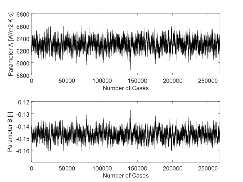
Figure 2: Markov chains obtained by MCMC.

6 Results and Discussion

6.1 Results via Markov Chain Monte Carlo

The posterior probability distribution obtained by MCMC of parameters $A$ and $B$ can be seen in Fig. 3. The 267000 states are represented, in this figure, by 20 bins, based on Doane’s formula [16]. Presenting a positive excess-kurtosis and skewness of $3\times$10^-2 each, these histograms are leptokurtic and approximately symmetrical.

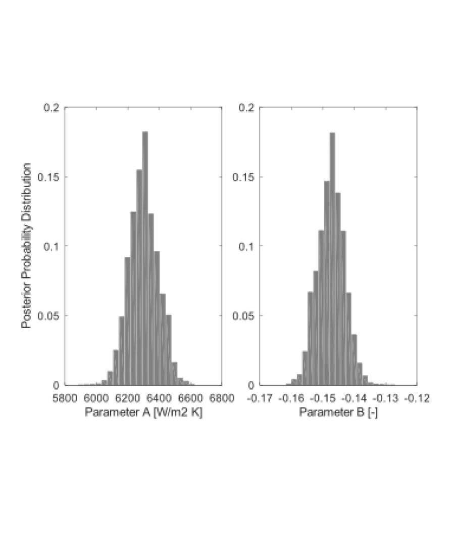
Figure 3: Histograms obtained by MCMC.

Based on Fig. 3, the parameter value that minimizes the model error with experimental data, ie, has the highest posterior probability value, is between 6200 and 6400 $\frac{\text{W}}{\text{m}^{2}\text{K}}$ for parameter $A$ and between -0.15 and -0.14 for parameter $B$. The expected value, such as percentile of 95%, 5% and standard deviation of the Markov Chain states are show in Tab. 2. Here, percentiles of 95% and 5% are denominated, respectively, the maximum and minimum value of each parameter.

Table 2: Expected value, standard deviation, maximum and minimum values of the parameters obtained by MCMC.

Parameter	Expected Value	Standard Deviation	Minimum Value	Maximum Value
A [W/m2 K]	6301	91	6126	6476
B [-]	-0.147	0.004	-0.156	-0.139

In Figure 4 is shown the numerical thermal profile resulted by the expected value of A and B obtained by MCMC. The small distance between the experimental and numerical curves corroborates the accuracy of the values raised for the heat exchange interface parameters. Applying the expected value obtained by MCMC in the simulatin, the standard deviation between the experimental and simulated thermal profile for the thermocouples in 4 mm, 8 mm and 12 mm were, respectively, 4.05 K, 3.72 K and 2.82 K.

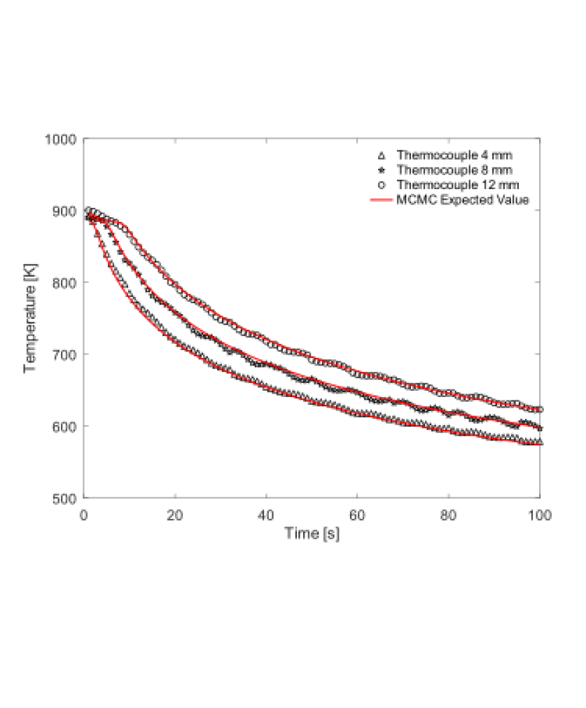
Figure 4: Experimental and simulated thermal profiles of Al-7wt.%Si solidification.

6.2 Performance Analysis of Metaheuristic Algorithms

In this section a performance analysis of all metaheuristic algorithms expressed on Section 3 is exposed. In order to present the results more coherently, this section will have four subsections: Sample Mean, Percentiles and Kurtosis (6.2.1), Error Analysis (6.2.2), Average Number of Iterations and Convergence (6.2.3) and Overall Performance (6.2.4).

An evaluation table of all the information present in this section can be seen in Tab. 3. The quantitative data were represented qualitatively based on parameters derived both from the information obtained by MCMC method and the performance of each metaheuristic algorithm. In this table, “Relative Performance” is based on the comparison of the results between the metaheuristic methods and MCMC. “Number of Iterations” stands for the average number of iterations of each optimizer. “Convergence” represents how the method was able to search the best minimum on the domain without being trapped on a local one. “Average Error” is a qualitative evaluation of the average error of the optimized values of each method under analysis. “Overall Performance” indicates a subjective evaluation of the authors about the results available during this research, taking into account all the metrics analyzed.

Table 3: Comparative performance analysis of the metaheuristic optimizers.

Methods	Relative Performance	Number of Iterations	Convergence	Average Error	Overral Performance
PSO	Excellent	High	Satisfactory	Low	Excellent
DE	Excellent	Medium	Good	Medium	Good
BA	Regular	Low	Premature	High	Regular
FPA	Regular	Low	Premature	High	Regular
GWO	Good	Medium	Satisfactory	Low	Excellent
MFO	Excellent	High	Satisfactory	Low	Excellent
SCA	Regular	Low	Premature	Medium	Regular
WOA	Regular	Medium	Good	Low	Good
DA	Regular	Low	Premature	Medium	Regular
HHO	Good	Low	Premature	High	Regular

6.2.1 Sample Mean, Percentiles and Kurtosis

In Figure 5, it is shown the quantitative results related to the studied optimizers. In this, the methods on the horizontal axis of the charts are in chronological sequence with respect to their publication. The horizontal lines represent the results obtained by MCMC. The circles represent the sample mean of the optimal values of each method, along with the standard deviation bars above and below that point. The second graphic shows the kurtosis of each method, in which the yellow horizontal line on the blue bars indicates the value 3, that guides the argument about tail size of the distribution presented in each method.

Figure 5: Uncertainty range and kurtosis of the metaheuristic methods and MCMC, for parameter $A$.

It is clear, based on the uncertainty range of each method, that all methods were able, at different coherence levels, to estimate the value of parameter $A$, considering the uncertainty range obtained by MCMC method. It is observed that, in a range from 0 to 10000 $\frac{\text{W}}{\text{m}^{2}\text{K}}$, the results of all methods are quite consistent, indicating that any method out of ten can retrieve the value of this parameter. However, some considerations can be taken from the chart:

• BA, FPA, and WOA presented a sample mean outside the uncertainty range of MCMC method. Considering the kurtosis of each method, it is observed that they do not recover exactly and precisely the expected value of MCMC. Even though the uncertainty range of each method covers part or all of MCMC uncertainty range, the probability that these methods will optimize the parameter to the exact range is quite small;

• PSO, GWO, SCA and DA presented a sample mean within MCMC uncertainty range, but exposed a wide range compared to the other methods, covering a region of approximately 2000 $\frac{\text{W}}{\text{m}^{2}\text{K}}$, or a small range that not cover all MCMC uncertainty range;

• Among the analyzed methods, DE, MFO and HHO stand out. The sample mean of these methods is quite consistent with the reference range and the standard deviation comprises a small range of values (even thought HHO does not presents a small range, its sample mean is very satisfactory, combined with a good kurtosis value). It is noteworthy the ability of MFO to recover, in a small uncertainty range and very high kurtosis, the optimal value of parameter $A$.

In Figure 6 is expressed the same quantitative parameters of statistical analysis as shown in Fig. 5, but relative to parameter $B$.

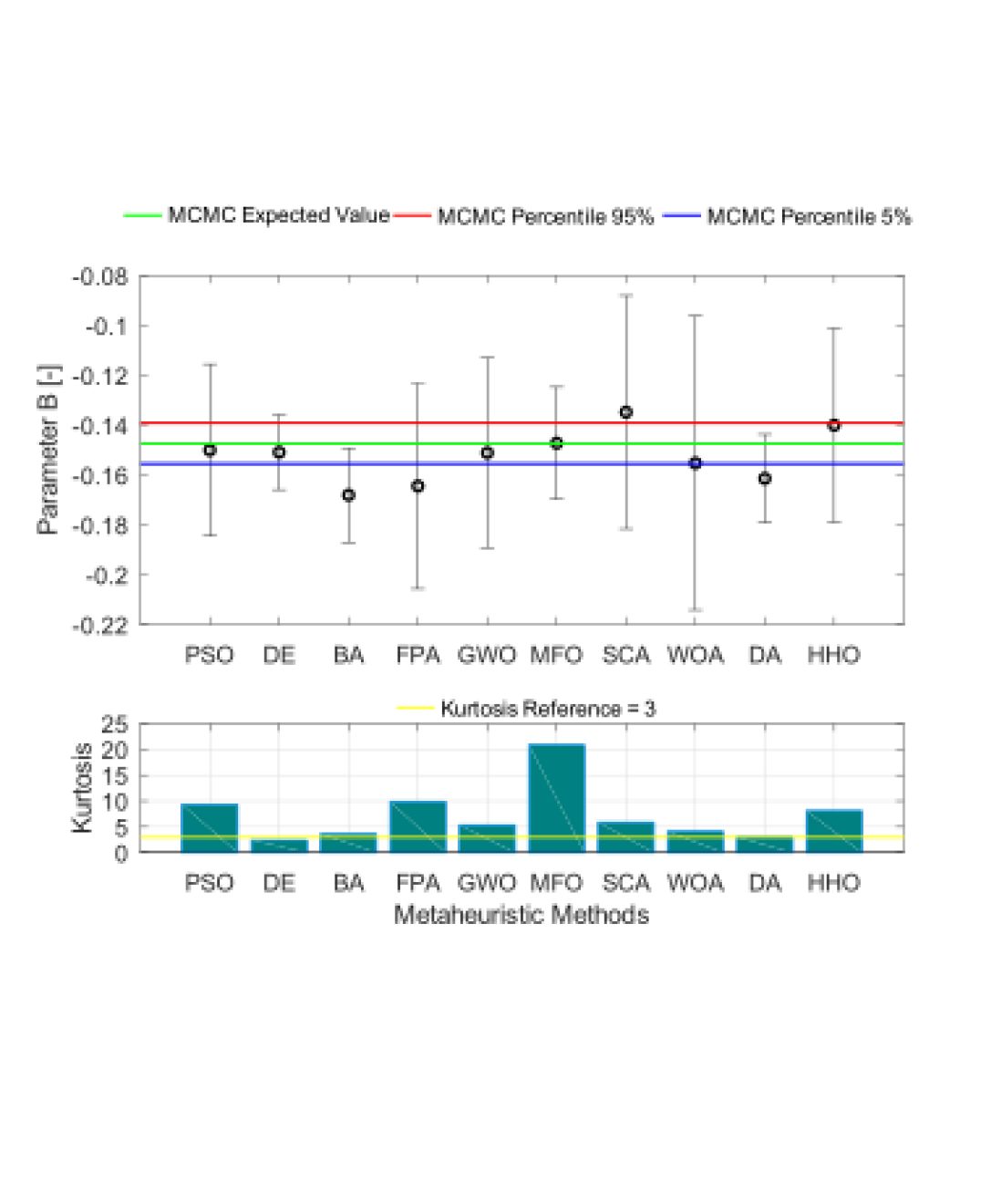
Figure 6: Uncertainty range and kurtosis of the metaheuristic methods and MCMC, for parameter $B$.

As expressed on parameter $A$ analysis, at different levels, all methods were able to estimate the value of parameter $B$, considering the MCMC uncertainty range. In the interval from -0.005 to -0.5, the results of all methods are consistent. However, it can be seen that the methods had greater difficulty in optimizing parameter $B$, which can be seen in the figure above. From the chart it is possible to visualize that:

• BA, FPA, SCA, WOA and DA presented a sample mean out of the uncertainty range of MCMC method. Even if WOA has a sample mean within the uncertainty range, the standard deviation presented is so large that it does not characterize the method satisfactorily.

• HHO presented a sample mean almost within MCMC uncertainty range, but exposed a very wide range compared to other methods (but not so wide as WOA);

• PSO, DE, GWO and MFO stand out. The consistency of the sample mean in relation to the reference range and the small standard deviation corroborate the excellent result of these methods. DE did not present high kurtosis value, but its performance is satisfactory. It is noteworthy the performance of MFO, which presented an almost exact sample mean and reaches a kurtosis value above 20. This indicates that MFO, besides being accurate, is extremely precise.

6.2.2 Error Analysis

In this subsection, the optimization errors of the metaheuristic algorithms under study will be analyzed. Consider, by notation, that $\mathcal{F}\left(\Box\right)$ is the fitness function and $\mathbf{G}_{*}$ is the vector that corresponds to the optimized values of each method. $\mathcal{F}\left(\mathbf{G}_{*}\right)$ stands for the error of each optimized parameter vector. Considering that we are evaluating three thermocouple positions and the error parameter is the standard deviation between experimental and numerical thermal profiles $\left(\sigma^{\text{therm}}_{i}\right)$, $\mathcal{F}\left(\mathbf{G}_{*}\right)$ can be represented as $\mathcal{F}\left(\mathbf{G}_{*}\right)=\sum_{1}^{3}\sigma^{\text{therm}}_{i}$.

Five metrics will be considered in terms of error: absolute sum $\left(\sum\mathcal{F}\left(\mathbf{G}_{*}\right)\right)$, expected value $\left(\text{E}\left[\mathcal{F}\left(\mathbf{G}_{*}\right)\right]\right)$, standard deviation $\left(\sigma\left(\mathcal{F}\left(\mathbf{G}_{*}\right)\right)\right)$ and maximum $\left(\text{max}\left(\mathcal{F}\left(\mathbf{G}_{*}\right)\right)\right)$ and minimum $\left(\text{min}\left(\mathcal{F}\left(\mathbf{G}_{*}\right)\right)\right)$ values. In Table 4 is shown the abovementioned metrics for each metaheuristic method analyzed.

Table 4: Absolute sum, expected value, standard deviation, maximum and minimum values of error for the metaheuristic algorithms under analysis.

Methods	$\sum\mathcal{F}\left(\mathbf{G}_{*}\right)$	$\text{E}\left[\mathcal{F}\left(\mathbf{G}_{*}\right)\right]$	$\sigma\left(\mathcal{F}\left(\mathbf{G}_{*}\right)\right)$	$\text{max}\left(\mathcal{F}\left(\mathbf{G}_{*}\right)\right)$	$\text{min}\left(\mathcal{F}\left(\mathbf{G}_{*}\right)\right)$
PSO	418.78	10.47	0.34	12.07	10.31
DE	447.49	11.19	0.79	13.40	10.34
BA	1030.30	25.76	18.05	78.89	10.66
FPA	960.91	24.02	16.15	84.36	10.80
GWO	420.71	10.52	0.15	10.91	10.32
MFO	413.71	10.34	0.05	10.60	10.31
SCA	469.8	11.75	1.31	14.75	10.41
WOA	428.56	10.71	0.61	13.19	10.32
DA	457.57	11.44	1.55	17.14	10.39
HHO	490.56	12.26	3.26	29.41	10.42

Considering only $\sum\mathcal{F}\left(\mathbf{G}_{*}\right)$ and $\text{E}\left[\mathcal{F}\left(\mathbf{G}_{*}\right)\right]$, it is possible to comment that:

• MFO, PSO, GWO and WOA, in this order, presented very good results, outperforming the other methods in these metrics. The data show that, on average, the optimization of these methods was quite satisfactory, reaching low error values and presenting a very low $\text{E}\left[\mathcal{F}\left(\mathbf{G}_{*}\right)\right]$, sometimes being less than the error obtained by the expected value of MCMC method;

• DE showed good results, such as low accumulated error and expected value. However, its expected value was almost 10% higher than the best result of this parameter (MFO), reducing its relative efficiency;

• DA, SCA, HHO, FPA and BA, in that order, presented unsatisfactory results in these metrics. In comparison with better performance methods, these presented very high values of accumulated error and expected error values of 1.1 to 2.5 times greater than the lowest expected value and accumulated error found (MFO).

Based on $\sigma\left(\mathcal{F}\left(\mathbf{G}_{*}\right)\right)$, $\text{max}\left(\mathcal{F}\left(\mathbf{G}_{*}\right)\right)$ and $\text{min}\left(\mathcal{F}\left(\mathbf{G}_{*}\right)\right)$, it is possible to argue that:

• MFO and GWO presented very small maximum intervals, indicating high precision. The two methods remained in the error range 10 to 11, providing the best results compared to all methods. The small standard deviation value presented by MFO is highlighted, which, corroborated by the high kurtosis presented in subsection 6.2.1, indicates that this method is the most accurate and precise of all;

• PSO and WOA showed good results such as small maximum interval and standard deviation. However, the maximum value presented by the two methods is at least 10 % higher than the lowest maximum values found (MFO);

• DE, SCA, DA, HHO, BA and FPA did not present satisfactory results. In addition to high standard deviation, their maximum value are 1.25 to 8 times greater than the best maximum value (MFO).

It is important to note that, due to the results of $\text{min}\left(\mathcal{F}\left(\mathbf{G}_{*}\right)\right)$, it is observed that at least in one optimization, all methods were able to satisfactorily minimize the parameters of the IHTC under study.

6.2.3 Average Number of Iterations and Convergence

In Figure 7 is shown the average number of iterations of each method until convergence. As stated in the Section 5, the stopping criterion considered in this paper is the repetition of the same parameter vector for 10 iterations.

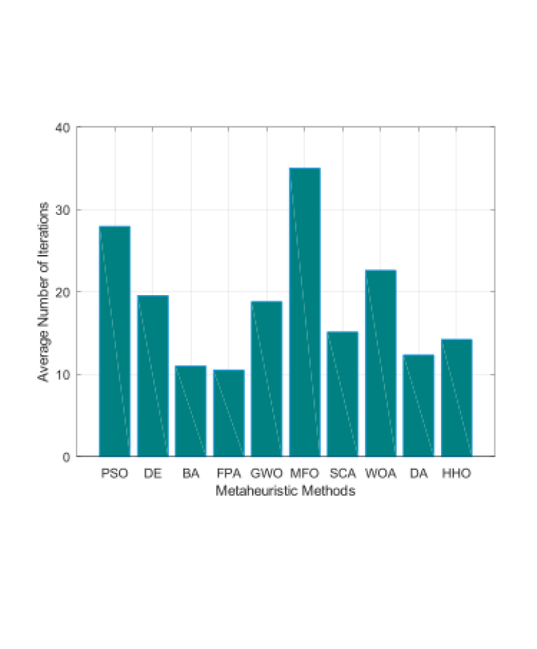
Figure 7: Average number of iterations for each optimization method.

It is possible to note from results that:

• BA, FPA, SCA, DA and HHO presented low average number of iterations, since the average of iterations were very close to the minimum stopping criterion. Given their poor performance shown in Figs. 5 and 6, it is possible to assume that this regular performance in parameter optimization indicates premature convergence;

• DE, GWO and WOA presented an average number of iterations twice greater than the stopping criterion.This is not necessarily a good thing. The price for the largest number of iterations should be rewarded with increased efficiency in finding a better critical point. In this case, the DE and WOA methods were good, with useful results. However, GWO showed a better iteration/result ratio among the three, with satisfactory convergence;

• Finally, PSO and MFO presented an average of iterations three times higher than the stopping criterion. This indicates that the search space was better explored. This actually corroborates the quantitative results. Even though the method required a higher average number of iterations, its results were quite satisfactory.

6.2.4 Overall Performance

From the previous analysis it is possible to draw conclusions about the parameter estimation in each metaheuristic method studied. One should keep in mind that the reference values used in this study are relative to MCMC results presented on Subsection 6.1 and .

Particle Swarm Optimization (PSO) presented excellent relative performance. The sample mean of parameters $A$ and $B$ was into the uncertainty range of reference and presented one of the highest excess-kurtosis for both parameters. PSO’s average number of iterations was high but it converged satisfactorily. In terms of error analysis, it presented the lowest minimum value of all methods and very good results, such as low expected value, accumulated error and standard deviation. It can be said, based on the above, that this method was one of the best in optimizing the IHTC parameters, presenting excellent overall performance.

Differential Evolution (DE) exposed excellent relative performance in both parameters under analysis. The uncertainty range produced by the method was consistent with the reference, indicating accuracy and precision. The average number of interactions was reasonable, indicating that the method did not show premature convergence. However, in the error analysis, it did not obtain as satisfactory results as other methods. In general, the method showed acceptable convergence and results. Thus, DE represents a good method to optimize this kind of physical problem.

Bat Algorithm (BA) showed regular relative performance in both parameters under analysis. The uncertainty interval produced by the method was quite inconsistent with the reference. This may be due to a very premature convergence, based on the average number of iterations, which has a value very close to the minimum number of acceptable iterations. This is reflected in the error analysis, which presented very bad metrics, both in accumulated error and expected value. Therefore, BA has not behaved as an adequate method for this type of inverse estimate in this case, showing regular overall performance.

Flower Pollination Algorithm (FPA) also presented regular relative performance in both parameters under analysis. The uncertainty range presented was quite inconsistent with the reference. This method, as BA, suffered very premature convergence, presenting a low number of iterations. In view of this, the error data presented by this method were not satisfactory. This presented a very high accumulated error, as well as expected value. That said, FPA had a regular overall performance.

Grey Wolf Optimizer (GWO) showed good relative performance. The uncertainty interval presented was consistent with the reference. The average number of iterations of this method was median, however it presented satisfactory convergence. This is demonstrated by the error analysis, which presented a low expected value and accumulated error. This presented one of the smallest maximum intervals among all methods, also standing out for the small standard deviation. Given this, GWO was one of the best methods analyzed, presenting excellent overall performance.

Moth-Flame Optimization (MFO) exposed excellent relative performance. The uncertainty range presented was quite consistent with the reference, both due to the proximity of the sample mean to the reference average and the small standard deviation presented. This fact is accentuated by the kurtosis of the distribution of the optimized parameters, higher than all the other methods. The average number of iterations of this method was high, however it presented very satisfactory convergence. In error analysis, MFO stood out. All the metrics presented by this model were the best, managing to be able to estimate as well, or even better, than the reference method itself. This presented the smallest maximum interval among all methods, also standing out for the small standard deviation. Given this, MFO was the best method analyzed, presenting a very satisfactory overall performance.

Sine Cosine Algorithm (SCA) presented regular relative performance. Its parameter uncertainty interval did not stand out when compared with the reference. The average number of iterations of this method was low and it showed premature convergence. When observing the performance through the error analysis, the algorithm presents median results, not as satisfactory as other methods analyzed. Based on the above, SCA presented itself as a regular method for this type of application.

Whale Optimization Algorithm (WOA) showed regular relative performance. The uncertainty range presented was quite bad compared to the reference. The standard deviation of the parameter estimate was one of the highest of all methods. The average number of iterations of this method was relatively high but presented acceptable convergence. By the error analysis, this method was satisfactory, presenting low average error in several metrics. Thus, WOA presented itself as a good method in this specific case.

Dragonfly Algorithm (DA) exposed regular relative performance. The uncertainty interval presented by the method, in both parameters under analysis, did not contain the reference interval. The average number of iterations of this method was small, which resulted in premature convergence and somewhat high error metrics. In view of these characteristics, DA did not present good results in general, being classified at the end as a regular method.

Harris Hawks Optimization (HHO) presented good relative performance. The uncertainty range exposed by the method was acceptable, with sample mean within the reference range and standard deviation, even though sharp, but with relative coherence with the reference range. However, the average number of iterations of this method was small, which resulted in premature convergence and high error metrics. In view of these characteristics, HHO did not present good results in comparison with the other methods, presenting itself as a regular method in this optimization application.

It is worth pointing out that some metaheuristic methods studied had difficulty in optimizing the parameters contained in the IHTC because the experimental data considered in this study are not smooth, presenting disturbances that create several local minimum near the optimal point. This enables premature convergence by creating dense local minimum zones. Therefore, the behavior of the metaheuristic methods considered in this paper may change when optimizing the same physical problem, but with smoother experimental data.

7 Conclusions

This paper presented a qualitative and quantitative performance analysis of ten nature-inspired metaheuristic algorithms in order to verify which metaheuristic method excels in the optimization of the Interfacial Heat Transfer Coefficient (IHTC) parameters in a unidirectional permanent mold casting process for Al-7wt.%Si alloy. For this purpose, was selected the optimizers: Particle Swarm Optimization (PSO), Differencial Evolution (DE), Bat Algorithm (BA), Flower Pollination Algorithm (FPA), Grey Wolf Optimizer (GWO), Moth-Flame Optimization (MFO), Sine Cosine Algorithm (SCA), Whale Optimization Algorithm (WOA), Dragonfly Algorithm (DA) and Harris Hawks Optimization (HHO). For that, a numerical discretization based on Finite Volume Method of the energy conservation equation in its integral form was taken into account [37]. It was considered, as uncertainty range of reference, simulated data extracted from the Markov Chain Monte Carlo (MCMC) method, from 267000 number of states, taken from 7 Markov chains initiated from different starting vectors. The considered IHTC in this analysis is the temporal function $A\left(t/t_{0}\right)^{B}$, where $A$ [$\frac{\text{W}}{\text{m}^{2}\text{K}}$] and $B$ [-] are constants, $t$ represents time [s] and $t_{0}$ a referential time [s] (here $t_{0}=1s$). The priori information of these methods were collected on [37]. This performance analysis considered as parameters for each metaheuristic method: Expected value, standard deviation and kurtosis (for parameters $A$ and $B$), average number of iterations, convergence and absolute sum, expected value, standard deviation, maximum and minimum value of the errors between numerical and experimental thermal profiles.

From the posterior probability distribution of MCMC, based on percentile 5 %, expected value and percentile 95 %, the optimal uncertainty range for parameter $A$ is, respectively, 6126 $\frac{\text{W}}{\text{m}^{2}\text{K}}$, 6301 $\frac{\text{W}}{\text{m}^{2}\text{K}}$ and 6476 $\frac{\text{W}}{\text{m}^{2}\text{K}}$ and, for parameter $B$, -0.156, -0.147 and -0.139. This range of uncertainty covers the a priori information collected by [37], validating it statistically.

Among the results obtained from the metaheuristic methods, it can be said that all of them would be able to reasonably optimize parameters $A$ and $B$. However, based on qualitative and quantitative metrics, BA, FPA SCA, DA and HHO did not present significant results. In general, these methods showed premature convergence, low correlation of the optimized values with the reference uncertainty range and high error values related to the optimized parameters. Thus, it can be said that these methods are not the most suitable for optimizing parameters in this specific problem.

On the other hand, DE and WOA showed reasonably good results, with adequate convergence, good average number of iterations and acceptable error metrics. They presented significantly superior results in relation to the aforementioned methods, however they did not provide a satisfactory level of error. Thus, it can be said that these methods provide good results when applied to this type of physical problem, however they are not the most suitable.

Unlike the others, PSO, GWO and MFO exposed promising results. These three presented the best quantitative results, well above the average of the previous methods. In general, the sample mean of these methods was very close to the reference expected value, their standard deviation was quite small when compared to the others, and kurtosis was quite high. The convergence of these three methods was satisfactory, with a reasonable average number of iterations. Their level of error were quite satisfactory, classifying them as excellent methods for this type of problem and application. It is important to note that MFO was the one that best optimized the parameters and reduced the uncertainty. This algorithm presented a very reduced uncertainty range, as well as the greater kurtosis. MFO was superior to the other methods in all error metrics, standing out even in comparison with the reference range itself. This fact shows that MFO is very accurated, presenting about 80% of the optimized points within the uncertainty range resulting from MCMC.

As PSO, GWO and especially MFO outperformed the other methods in different quantitative parameters, they have total potential to optimize the IHTC parameters $A$ and $B$ coupled in the solidification phenomenon applied in the permanent metal mold casting. Then, all of them can be used without loss of accuracy and precision. Finally, it is worthy pointing out that the performance of all the methods analyzed in this article is extremely influenced by the values of the constants intrinsic to the numerical methodology. Thus, research on the best values to be used in the constants is encouraged in order to expand the applicability and efficiency of numerical methods in engineering and metallurgy applications such as the one studied in this contribution.

References

- [1] Flocks, herds and schools: A distributed behavioral model, volume 21. ACM, 1987.
- [2] O. Abdalla, H. Rezk, and E. M. Ahmed. Wind driven optimization algorithm based global mppt for pv system under non-uniform solar irradiance. Solar Energy, 180:429–444, 2019.
- [3] M. Abdullah, N. Javaid, I. U. Khan, Z. A. Khan, A. Chand, and N. Ahmad. Optimal power flow with uncertain renewable energy sources using flower pollination algorithm. In International Conference on Advanced Information Networking and Applications, pages 95–107. Springer, 2019.
- [4] I. Babuška, Z. Sawlan, M. Scavino, B. Szabó, and R. Tempone. Bayesian inference and model comparison for metallic fatigue data. Computer Methods in Applied Mechanics and Engineering, 304:171–196, 2016.
- [5] Z. Bayraktar, M. Komurcu, J. A. Bossard, and D. H. Werner. The wind driven optimization technique and its application in electromagnetics. IEEE transactions on antennas and propagation, 61(5):2745–2757, 2013.
- [6] A. Benamor, M. Benchouia, K. Srairi, and M. Benbouzid. A new rooted tree optimization algorithm for indirect power control of wind turbine based on a doubly-fed induction generator. ISA transactions, 88:296–306, 2019.
- [7] A. Beşkirli, D. Özdemir, and H. Temurtaş. A comparison of modified tree–seed algorithm for high-dimensional numerical functions. Neural Computing and Applications, pages 1–35, 2019.
- [8] C. Brito, T. A. Costa, T. A. Vida, F. Bertelli, N. Cheung, J. E. Spinelli, and A. Garcia. Characterization of dendritic microstructure, intermetallic phases, and hardness of directionally solidified al-mg and al-mg-si alloys. Metallurgical and Materials Transactions A, 46(8):3342–3355, 2015.
- [9] S. Chen, K. Liu, and X.-G. Chen. Effect of mo on elevated-temperature low-cycle fatigue behavior of al-si 356 cast alloy. In Light Metals 2020, pages 261–266. Springer, 2020.
- [10] Z. Chen et al. Bayesian filtering: From kalman filters to particle filters, and beyond. Statistics, 182(1):1–69, 2003.
- [11] Z. Cheng and H. Wang. How to control the crack to propagate along the specified path feasibly? Computer Methods in Applied Mechanics and Engineering, 336:554–577, 2018.
- [12] A. Cheraghalipour, M. Hajiaghaei-Keshteli, and M. M. Paydar. Tree growth algorithm (tga): A novel approach for solving optimization problems. Engineering Applications of Artificial Intelligence, 72:393–414, 2018.
- [13] R. Chi, Y.-x. Su, D.-h. Zhang, X.-x. Chi, and H.-j. Zhang. A hybridization of cuckoo search and particle swarm optimization for solving optimization problems. Neural Computing and Applications, 31(1):653–670, 2019.
- [14] V. Courchelle, M. Soler, D. González-Arribas, and D. Delahaye. A simulated annealing approach to 3d strategic aircraft deconfliction based on en-route speed changes under wind and temperature uncertainties. Transportation Research Part C: Emerging Technologies, 103:194–210, 2019.
- [15] E. H. de Vasconcelos Segundo, V. C. Mariani, and L. dos Santos Coelho. Design of heat exchangers using falcon optimization algorithm. Applied Thermal Engineering, 156:119 – 144, 2019.
- [16] D. P. Doane. Aesthetic frequency classifications. The American Statistician, 30(4):181–183, 1976.
- [17] M. Dorigo and G. Di Caro. Ant colony optimization: a new meta-heuristic. In Proceedings of the 1999 congress on evolutionary computation-CEC99 (Cat. No. 99TH8406), volume 2, pages 1470–1477. IEEE, 1999.
- [18] N. El-Mahallawy and A. Assar. Effect of melt superheat on heat transfer coefficient for aluminium solidifying against copper chill. Journal of Materials Science, 26(7):1729–1733, 1991.
- [19] A. E. Ezugwu, O. J. Adeleke, A. A. Akinyelu, and S. Viriri. A conceptual comparison of several metaheuristic algorithms on continuous optimisation problems. Neural Computing and Applications, pages 1–45, 2019.
- [20] N. Gnanasekaran and C. Balaji. Markov chain monte carlo (mcmc) approach for the determination of thermal diffusivity using transient fin heat transfer experiments. International Journal of Thermal Sciences, 63:46–54, 2013.
- [21] G. Hanrahan. Swarm intelligence metaheuristics for enhanced data analysis and optimization. Analyst, 136(18):3587–3594, 2011.
- [22] A. A. Heidari, S. Mirjalili, H. Faris, I. Aljarah, M. Mafarja, and H. Chen. Harris hawks optimization: Algorithm and applications. Future Generation Computer Systems, 97:849–872, 2019.
- [23] S. C. Johnson, C. D. Clark, and J. S. Alvarez. Development and analysis of al7075 alloy materials using press and sinter processing. In Light Metals 2020, pages 233–240. Springer, 2020.
- [24] T. Joyce and J. M. Herrmann. A review of no free lunch theorems, and their implications for metaheuristic optimisation. In Nature-Inspired Algorithms and Applied Optimization, pages 27–51. Springer, 2018.
- [25] J. Kennedy and R. Eberhart. Particle swarm optimization: Proceedings. In IEEE international conference on neural networks, volume 4, pages 1942–1948. Piscataway NJ, IEEE Service Center, 1995.
- [26] M. S. Kiran. Tsa: Tree-seed algorithm for continuous optimization. Expert Systems with Applications, 42(19):6686–6698, 2015.
- [27] S. Kirkpatrick, C. D. Gelatt, and M. P. Vecchi. Optimization by simulated annealing. Science, 220(4598):671–680, 1983.
- [28] A. Kordijazi, S. K. Behera, O. Akbarzadeh, M. Povolo, and P. Rohatgi. A statistical analysis to study the effect of silicon content, surface roughness, droplet size and elapsed time on wettability of hypoeutectic cast aluminum–silicon alloys. In Light Metals 2020, pages 185–193. Springer, 2020.
- [29] H. Kumar and G. Nagarajan. A bayesian inference approach: estimation of heat flux from fin for perturbed temperature data. Sādhanā, 43(4):62, 2018.
- [30] S. Lakshmanaprabu, K. Shankar, S. S. Rani, E. Abdulhay, N. Arunkumar, G. Ramirez, and J. Uthayakumar. An effect of big data technology with ant colony optimization based routing in vehicular ad hoc networks: Towards smart cities. Journal of Cleaner Production, 217:584–593, 2019.
- [31] J. McDermott. When and why metaheuristics researchers can ignore “no free lunch” theorems. Metaheuristics, pages 1–18, 2019.
- [32] S. Mirjalili. Moth-flame optimization algorithm: A novel nature-inspired heuristic paradigm. Knowledge-Based Systems, 89:228–249, 2015.
- [33] S. Mirjalili. Dragonfly algorithm: a new meta-heuristic optimization technique for solving single-objective, discrete, and multi-objective problems. Neural Computing and Applications, 27(4):1053–1073, 2016.
- [34] S. Mirjalili. Sca: a sine cosine algorithm for solving optimization problems. Knowledge-Based Systems, 96:120–133, 2016.
- [35] S. Mirjalili and A. Lewis. The whale optimization algorithm. Advances in Engineering Software, 95:51–67, 2016.
- [36] S. Mirjalili, S. M. Mirjalili, and A. Lewis. Grey wolf optimizer. Advances in Engineering Software, 69:46–61, 2014.
- [37] E. P. Oliveira, G. M. Stieven, E. F. Lins, and J. R. P. Vaz. An inverse approach for the interfacial heat transfer parameters in alloys solidification. Applied Thermal Engineering, 155:365–372, 2019.
- [38] H. R. Orlande, O. Fudym, D. Maillet, and R. M. Cotta. Thermal measurements and inverse techniques. CRC Press, 2011.
- [39] M. D. Peres. Desenvolvimento da macroestrutura e da microestrutura na solidificação unidirecional transitoria de ligas Al-Si. Doctoral thesis, Federal University of Campinas, 2005.
- [40] J. Rakhmonov, G. Timelli, F. Bonollo, and L. Arnberg. Influence of grain refiner addition on the precipitation of fe-rich phases in secondary alsi7cu3mg alloys. International Journal of Metalcasting, 11(2):294–304, 2017.
- [41] M. Samy, S. Barakat, and H. Ramadan. A flower pollination optimization algorithm for an off-grid pv-fuel cell hybrid renewable system. International Journal of Hydrogen Energy, 44(4):2141–2152, 2019.
- [42] G. Santos, P. Goulart, A. Couto, and A. Garcia. Primary dendrite arm spacing effects upon mechanical properties of an al–3wt% cu–1wt% li alloy. In Properties and Characterization of Modern Materials, pages 215–229. Springer, 2017.
- [43] O. Satbhai, S. Roy, and S. Ghosh. A parametric multi-scale, multiphysics numerical investigation in a casting process for al-si alloy and a macroscopic approach for prediction of ect and cet events. Applied Thermal Engineering, 113:386–412, 2017.
- [44] S. Shadravan, H. Naji, and V. K. Bardsiri. The sailfish optimizer: A novel nature-inspired metaheuristic algorithm for solving constrained engineering optimization problems. Engineering Applications of Artificial Intelligence, 80:20–34, 2019.
- [45] Z. Shao, D. Pi, and W. Shao. A novel multi-objective discrete water wave optimization for solving multi-objective blocking flow-shop scheduling problem. Knowledge-Based Systems, 165:110–131, 2019.
- [46] G. Sigworth. Aluminum Casting Alloys and Casting Processes. In Aluminum Science and Technology. ASM International, 2018.
- [47] G. Sigworth. Solidification and Castability of Foundry Alloys. In Aluminum Science and Technology. ASM International, 2018.
- [48] J. E. Spinelli, N. Cheung, P. R. Goulart, J. M. Quaresma, and A. Garcia. Design of mechanical properties of al-alloys chill castings based on the metal/mold interfacial heat transfer coefficient. International Journal of Thermal Sciences, 51:145 – 154, 2012.
- [49] R. Storn. On the usage of differential evolution for function optimization. In Proceedings of North American Fuzzy Information Processing, pages 519–523. IEEE, 1996.
- [50] R. Storn and K. Price. Differential evolution - a simple and efficient heuristic for global optimization over continuous spaces. Journal of Global Optimization, 11(4):341–359, 1997.
- [51] J. Stroh, A. Piche, D. Sediako, A. Lombardi, and G. Byczynski. The effects of solidification cooling rates on the mechanical properties of an aluminum inline-6 engine block. In Light Metals 2019, pages 505–512. Springer, 2019.
- [52] S. Szénási and I. Felde. Using multiple graphics accelerators to solve the two-dimensional inverse heat conduction problem. Computer Methods in Applied Mechanics and Engineering, 336:286–303, 2018.
- [53] K. S. Tey, S. Mekhilef, and M. Seyedmahmoudian. Implementation of bat algorithm as maximum power point tracking technique for photovoltaic system under partial shading conditions. In 2018 IEEE Energy Conversion Congress and Exposition (ECCE), pages 2531–2535. IEEE, 2018.
- [54] P. Vishweshwara, N. Gnanasekaran, and M. Arun. Inverse estimation of interfacial heat transfer coefficient during the solidification of sn-5wt% pb alloy using evolutionary algorithm. In Advances in Materials and Metallurgy, pages 227–237. Springer, 2019.
- [55] H. Wang, M. Hamed, and S. Shankar. Interaction between primary dendrite arm spacing and velocity of fluid flow during solidification of al–si binary alloys. Journal of Materials Science, 53:9771–9789, 07 2018.
- [56] D. H. Wolpert, W. G. Macready, et al. No free lunch theorems for search. Technical report, Technical Report SFI-TR-95-02-010, Santa Fe Institute, 1995.
- [57] D. H. Wolpert, W. G. Macready, et al. No free lunch theorems for optimization. IEEE Transactions on Evolutionary Computation, 1(1):67–82, 1997.
- [58] Y. Xue, J. Jiang, B. Zhao, and T. Ma. A self-adaptive artificial bee colony algorithm based on global best for global optimization. Soft Computing, pages 1–18, 2018.
- [59] X.-S. Yang. A new metaheuristic bat-inspired algorithm. In Nature inspired cooperative strategies for optimization (NICSO 2010), pages 65–74. Springer, 2010.
- [60] X.-S. Yang. Flower pollination algorithm for global optimization. In International conference on unconventional computing and natural computation, pages 240–249. Springer, 2012.
- [61] X.-S. Yang. Free lunch or no free lunch: that is not just a question? International Journal on Artificial Intelligence Tools, 21(03):1240010, 2012.
- [62] X.-S. Yang. Nature-inspired optimization algorithms. Elsevier, 2014.
- [63] X.-S. Yang. Mathematical analysis of nature-inspired algorithms. In Nature-Inspired Algorithms and Applied Optimization, pages 1–25. Springer, 2018.
- [64] X.-S. Yang and S. Deb. Cuckoo search via lévy flights. In 2009 World Congress on Nature & Biologically Inspired Computing (NaBIC), pages 210–214. IEEE, 2009.
- [65] L. Zeng, W. Zhang, Y. Ji, Y. Huang, and J. Li. Improving cooling rate during solidification by eliminating the metal–mold interfacial gap. Metallurgical and Materials Transactions A, 46(7):2819–2822, 2015.
- [66] W. Zhao, Z. Zhang, and L. Wang. Manta ray foraging optimization: An effective bio-inspired optimizer for engineering applications. Engineering Applications of Artificial Intelligence, 87:103300, 2020.
- [67] Y.-J. Zheng. Water wave optimization: a new nature-inspired metaheuristic. Computers & Operations Research, 55:1–11, 2015.