Quadratic Word Equations with Length Constraints, Counter Systems, and Presburger Arithmetic with Divisibility

Abstract.

Word equations are a crucial element in the theoretical foundation of constraint solving over strings. A word equation relates two words over string variables and constants. Its solution amounts to a function mapping variables to constant strings that equate the left and right hand sides of the equation. While the problem of solving word equations is decidable, the decidability of the problem of solving a word equation with a length constraint (i.e., a constraint relating the lengths of words in the word equation) has remained a long-standing open problem. We focus on the subclass of quadratic word equations, i.e., in which each variable occurs at most twice. We first show that the length abstractions of solutions to quadratic word equations are in general not Presburger-definable. We then describe a class of counter systems with Presburger transition relations which capture the length abstraction of a quadratic word equation with regular constraints. We provide an encoding of the effect of a simple loop of the counter systems in the existential theory of Presburger Arithmetic with divisibility (PAD).

Since PAD is decidable (NP-hard and is in NEXP), we obtain a decision procedure for quadratic words equations with length constraints for which the associated counter system is flat (i.e., all nodes belong to at most one cycle). In particular, we show a decidability result (in fact, also an NP algorithm with a PAD oracle) for a recently proposed NP-complete fragment of word equations called regular-oriented word equations, when augmented with length constraints. We extend this decidability result (in fact, with a complexity upper bound of PSPACE with a PAD oracle) in the presence of regular constraints.

1. Introduction

Reasoning about strings is a fundamental problem in computer science and mathematics. The first order theory over strings and concatenation is undecidable. A seminal result by Makanin [Mak77] (see also [Die02, J1́3]) shows that the satisfiability problem for the existential fragment is decidable, by giving an algorithm for the satisfiability of word equations. A word equation $L=R$ consists of two words $L$ and $R$ over an alphabet of constants and variables. It is satisfiable if there is a mapping $\sigma$ from the variables to strings over the constants such that $\sigma(L)$ and $\sigma(R)$ are syntactically identical.

An original motivation for studying word equations was to show undecidability of Hilbert’s 10th problem (see, e.g., [Mat68]). This was motivated among others by an earlier result by Quine [Qui46] that first-order theory over word equations essentially coincides with first-order theory of arithmetic. While Makanin’s later result shows that word equations could not, by themselves, show undecidability, Matiyasevich in 1968 considered an extension of word equations with length constraints as a possible route to showing undecidability of Hilbert’s 10th problem [Mat68]. A length constraint constrains the solution of a word equation by requiring a linear relation to hold on the lengths of words in a solution $\sigma$ (e.g., $|x|=|y|$, where $|\cdot|$ denotes the string-length function). The decidability of word equations with length constraints remains open.

In recent years, reasoning about strings with length constraints has found renewed interest through applications in program verification and reasoning about security vulnerabilities. The focus of most research has been on developing practical string solvers (cf. [YABI14, TCJ14, BTV09, AAC⁺14, LRT⁺14, K⁺12, BGZ17, HJL⁺18, WTL⁺16, SAH⁺10]). These solvers are sound but make no claims of completeness. Relatively few results are known about the decidability status of strings with length and other constraints (see [D⁺18] for an overview of the results in this area). The main idea in most existing decidability results is the encoding of length constraints into Presburger arithmetic [G⁺13, D⁺18, AAC⁺14, LB16]. However, as we shall see in this paper, the length abstraction of a word equation (i.e. the set of possible lengths of variables in its solutions) need not be Presburger definable.

In this paper, we consider the case of quadratic word equations, in which each variable can appear at most twice [Len72, DR99], together with length constraints and regular constraints (conjunctions $\bigwedge_{i=1}^{n}x\in L_{i}$ of assertions that the variable $x$ must be assigned a string in the regular language $L_{i}$ for each $i$). For quadratic word equations, there is a simpler decision procedure (called the Nielsen transform or Levi’s method) based on a non-deterministic proof graph construction. The technique can be extended to handle regular constraints [DR99]. However, we show that already for this class (even for a simple equation like $xaby=yabx$, where $x,y$ are variables and $a,b$ are constants), the length abstraction need not be Presburger-definable. Thus, techniques based on Presburger encodings are not sufficient to prove decidability.

Our first observation in this paper is a connection between the problem of quadratic word equations with length constraints and a class of terminating counter systems with Presburger transitions. Informally, the counter system has control states corresponding to the nodes of the proof graph constructed by Levi’s method, and a counter standing for the length of a word variable. Each counter value either remains the same or gets decreased in each step of Levi’s method. When all of the counters remain the same, the counter system goes to a state, from which the previous state can no longer be visited. Thus, from any initial state, the counter system terminates. We show that the set of initial counter values which can lead to a successful leaf (i.e., one containing the trivial equation $\epsilon=\epsilon$) is precisely the length abstraction of the word equation.

Our second observation is that the reachability relation for a simple loop of the counter system can be encoded in the existential theory of Presburger arithmetic with divisibility (PAD). As PAD is decidable [Lip76, LOW15], we obtain a technique to symbolically represent the reachability relation for flat counter systems, in which each node belongs to at most one loop.

Moreover, the same encoding shows decidability for word equations with length constraints, provided the proof tree is associated with flat counter systems. In particular, we show that the class of regular-oriented word equations, introduced by [DMN17], have flat proof graphs. Thus, the satisfiability problem for quadratic regular-oriented word equations with length constraints is decidable. In fact, we obtain an NP algorithm with an oracle access to PAD; the best complexity bound for the latter is NEXP and NP-hardness [LOW15]. A standard monoid technique for handling regular constraints in word equations (e.g. see [DR99]) can then be used to extend our decidability result in the presence of regular constraints. This results in a PSPACE algorithm with an oracle access to PAD.

While our decidability result is for a simple subclass, this class is already non-trivial without length and regular constraints: satisfiability of regular-oriented word equations is NP-complete [DMN17]. Notice that in the presence of regular constraints the complexity (without length constraints, and even without word equations) jumps to PSPACE, by virtue of the standard PSPACE-completeness of intersection of regular languages [Koz77]. Moreover, we believe that the techniques in this paper — the connection between acceleration and word equations, and the use of existential Presburger with divisibility — can pave the way to more sophisticated decision procedures based on counter system acceleration.

2. Preliminaries

General notation: Let $\mathbb{N}=\mathbb{Z}_{\geq 0}$ be the set of all natural numbers. For integers $i\leq j$, we use $[i,j]$ to denote the set $\{i,i+1,\ldots,j-1,j\}$ of integers. If $i\in\mathbb{N}$, let $[i]$ denote $[0,i]$. We use $\preceq$ to denote the component-wise ordering on $\mathbb{N}^{k}$, i.e., $(x_{1},\ldots,x_{k})\preceq(y_{1},\ldots,y_{k})$ iff $x_{i}\leq y_{i}$ for all $i\in[1,k]$. If $\bar{x}\preceq\bar{y}$ and $\bar{x}\neq\bar{y}$, we write $\bar{x}\prec\bar{y}$.

If $S$ is a set, we use $S^{*}$ to denote the set of all finite sequences, or words, $\gamma=s_{1}\ldots s_{n}$ over $S$. The length $|\gamma|$ of $\gamma$ is $n$. The empty sequence is denoted by $\epsilon$. Notice that $S^{*}$ forms a monoid with the concatenation operator $\cdot$. If $\gamma^{\prime}$ is a prefix of $\gamma$, we write $\gamma^{\prime}\preceq\gamma$. Additionally, if $\gamma^{\prime}\neq\gamma$ (i.e. a strict prefix of $\gamma$), we write $\gamma^{\prime}\prec\gamma$. Note that the operator $\preceq$ is overloaded here, but the meaning should be clear from the context.

Words and automata: We assume basic familiarity with word combinatorics and automata theory. Fix a (finite) alphabet $A$. For each finite word $w:=w_{1}\ldots w_{n}\in A^{*}$, we write $w[i,j]$, where $1\leq i\leq j\leq n$, to denote the segment $w_{i}\ldots w_{j}$.

Two words $x$ and $y$ are conjugates if there exist words $u$ and $v$ such that $x=uv$ and $y=vu$. Equivalently, $x=\mathrm{cyc}^{k}(y)$ for some $k$ and for the cyclic permutation operation $\mathrm{cyc}:A^{*}\rightarrow A^{*}$, defined as $\mathrm{cyc}(\epsilon)=\epsilon$, and $\mathrm{cyc}(a\cdot w)=w\cdot a$ for $a\in A$ and $w\in A^{*}$.

Given a nondeterministic finite automaton (NFA) $\mathcal{A}:=(A,Q,\Delta,q_{0},{{F}})$, where $\Delta\subseteq Q\times A\times Q$, a run of $\mathcal{A}$ on $w=a_{1}\cdots a_{n}$ is a function $\rho:[0,n]\to Q$ with $\rho(0)=q_{0}$ that obeys the transition relation $\Delta$: $(\rho(i),a_{i+1},\rho(i+1))\in\Delta$, for all $i\in[0,n-1]$. We may also denote the run $\rho$ by the word $\rho(0)\cdots\rho(n)$ over the alphabet $Q$. The run $\rho$ is said to be accepting if $\rho(n)\in F$, in which case we say that the word $w$ is accepted by $\mathcal{A}$. The language $\mathcal{L}(\mathcal{A})$ of $\mathcal{A}$ is the set of words in $A^{*}$ accepted by $\mathcal{A}$. In the sequel, for $p,q\in Q$ we will write $\mathcal{A}_{p,q}$ to denote the NFA $\mathcal{A}$ with initial state replaced by $p$ and final state replaced by $q$.

Word equations: Let $A$ be a (finite) alphabet of constants and ${V}$ a set of variables; we assume $A\cap{V}=\emptyset$. A word equation $E$ is an expression of the form $L=R$, where $(L,R)\in(A\cup{V})^{*}\times(A\cup{V})^{*}$. A system of word equations is a nonempty set ${\{L_{1}=R_{1},L_{2}=R_{2},\ldots,L_{k}=R_{k}\}}$ of word equations. The length of a system of word equations is the length $\sum_{i=1}^{k}(|L_{i}|+|R_{i}|)$. A system is called quadratic if each variable occurs at most twice in the entire system. A solution to a system of word equations is a homomorphism ${\sigma}:(A\cup{V})^{*}\rightarrow A^{*}$ which maps each $a\in A$ to itself that equates the l.h.s. and r.h.s. of each equation, i.e., ${\sigma}(L_{i})={\sigma}(R_{i})$ for each $i=1,\ldots,k$.

For each variable $x\in{V}$, we shall use $|x|$ to denote a formal variable that stands for the length of variable $x$, i.e., for any solution $\sigma$, the formal variable $|x|$ takes the value $|\sigma(x)|$. Let $L_{{V}}$ be the set ${\{|x|\mid x\in{V}\}}$. A length constraint is a formula in Presburger arithmetic whose free variables are in $L_{V}$.

A solution to a system of word equations with a length constraint $\Phi(|{x_{1}}|,\ldots,|{x_{n}}|)$ is a homomorphism ${\sigma}:(A\cup{V})^{*}\rightarrow A^{*}$ which maps each $a\in A$ to itself such that ${\sigma}(L_{i})={\sigma}(R_{i})$ for each $i=1,\ldots,k$ and moreover $\Phi(|{\sigma}(x_{1})|,\ldots,|{\sigma}(x_{n})|)$ holds. That is, the homomorphism maps each variable to a word in $A^{*}$ such that each word equation is satisfied, and the lengths of these words satisfy the length constraint.

The satisfiability problem for word equations with length constraints asks, given a system of word equations and a length constraint, whether it has a solution.

We also consider the extension of the problem with regular constraints. For a system of word equations, a variable $x\in{V}$, and a regular language $\mathcal{L}\subseteq A^{*}$, a regular constraint $x\in\mathcal{L}$ imposes the additional restriction that any solution ${\sigma}$ must satisfy ${\sigma}(x)\in\mathcal{L}$. Given a system of word equations, a length constraint, and a set of regular constraints, the satisfiability problem asks if there is a solution satisfying the word equation, the length constraints, as well as the regular constraints.

In this paper we consider only a system consisting of a single word equation. We note quickly that there are various possible satisfiability-preserving reductions that reduce a system of word equations to a single word equation (e.g. [KMP00]), but most of them do not in general preserve desirable properties such as the quadraticity of the constraints. One simple method that preserves the quadraticity of the constraints is to simply concatenate the left/right hand sides of the equations and simply introduce some length constraints. For example, suppose we have constraints $xy=yz\wedge zz_{1}=z_{1}z_{2}\wedge|x|=|z_{2}|$. The resulting constraint involving only a single word equation would be $xyzz_{1}=yzz_{1}z_{2}\wedge|x|=|z_{2}|\wedge|x|+|y|=|y|+|z|$. In general, even this reduction does not preserve the properties that we consider in this paper (flatness, regularity, orientedness), unless further restrictions are imposed. See Section 5 for the definitions. We will remark this further in the relevant parts of the paper.

Linear arithmetic with divisibility: Let $\mathcal{P}$ be a first-order language over the domain $\mathbb{N}$ of natural numbers with equality = and inequality $\leq$ of numbers relations, and with terms being linear polynomials with integer coefficients. We write $f(x)$, $g(x)$, etc., for terms in integer variables $x=x_{1},\ldots,x_{n}$. Atomic formulas in Presburger arithmetic have the form $f(x)\leq g(x)$ or $f(x)=g(x)$. The language PAD of Presburger arithmetic with divisibility extends the language $\mathcal{P}$ with a binary relation $|$ (for divides). An atomic formula has the form $f(x)\leq g(x)$ or $f(x)=g(x)$ or $f(x)|g(x)$, where $f(x)$ and $g(x)$ are linear polynomials with integer coefficients. The full first order theory of PAD is undecidable, but the existential fragment is decidable [Lip76, LOW15].

Note that the divisibility predicate $x|y$ is not expressible in Presburger arithmetic: a simple way to see this is that ${\{(x,y)\in\mathbb{N}^{2}\mid x|y\}}$ is not a semi-linear set.

Counter systems: In this paper, we specifically use the term “counter systems” to mean counter systems with Presburger transition relations (e.g. see [BFLP08]). These more general transition relations can be simulated by standard Minsky’s counter machines, but they are more useful for coming up with decidable subclasses of counter systems. A counter system $\mathcal{C}$ is a tuple $(X,Q,\Delta)$, where $X=\{x_{1},\ldots,x_{m}\}$ is a finite set of counters, $Q$ is a finite set of control states, and $\Delta$ is a finite set of transitions of the form $(q,\Phi(\bar{}x,\bar{}x^{\prime}),q^{\prime})$, where $q,q^{\prime}\in Q$ and $\Phi$ is a Presburger formula with free variables $x_{1},\ldots,x_{m},x_{1}^{\prime},\ldots,x_{m}^{\prime}$. A configuration of $\mathcal{C}$ is a tuple $(q,\text{\rm v})\in Q\times\mathbb{N}^{m}$.

The semantics of counter systems is given as a transition system. A transition system is a tuple $\mathfrak{S}:=\langle S;\to\rangle$, where $S$ is a set of configurations and $\to\ \subseteq S\times S$ is a binary relation over $S$. A path in $\mathfrak{S}$ is a sequence $s_{0}\to\cdots\to s_{n}$ of configurations $s_{0},...,s_{n}\in S$. If $S^{\prime}\subseteq S$, let ${\rm Phys.~{}Rev.~{}E}^{*}(S^{\prime})$ denote the set of $s\in S$ such that $s\to^{*}s^{\prime}$ for some $s^{\prime}\in S^{\prime}$. We might write ${\rm Phys.~{}Rev.~{}E}_{\to}^{*}(S^{\prime})$ to disambiguate the transition system.

A counter system $\mathcal{C}$ generates the transition system $\mathfrak{S}_{\mathcal{C}}=\langle S;\to\rangle$, where $S$ is the set of all configurations of $\mathcal{C}$, and $(q,\text{\rm v})\to(q^{\prime},\text{\rm v}^{\prime})$ if there exists a transition $(q,\Phi(\bar{}x,\bar{}x^{\prime}),q^{\prime})\in\Delta$ such that $\Phi(\text{\rm v},\text{\rm v}^{\prime})$ is true.

In the sequel, we will be needing the notion of flat counter systems [BIL09, LS06, BFLS05, BFLP08]. Given a counter system $\mathcal{C}=(X,Q,\Delta)$, the control structure of $\mathcal{C}$ is an edge-labeled directed graph $G=(V,E)$ with the set $V=Q$ of nodes and the set $E=\Delta$. The counter system $\mathcal{C}$ is flat if each node $v\in V$ is contained in at most one simple cycle. We now define the notion of “skeletons” in $\mathcal{C}$, which we will use in Section 5. Intuitively, a skeleton is simply a simple path with simple cycles along the way in the graph $\mathcal{C}$. More precisely, considering $\mathcal{C}$ a dag of SCCs, we define the signature $s_{\mathcal{C}}$ of $\mathcal{C}$ as the (directed) graph whose nodes are SCCs in $\mathcal{C}$ and there is an edge from $v$ to $w$ if there is a state in the SCC $v$ that can go to a state in SCC $w$. A skeleton in $\mathcal{C}$ is simply a subgraph $G^{\prime}=(V^{\prime},E^{\prime})$ of $\mathcal{C}$ that is obtained by taking a (simple) path in $s_{\mathcal{C}}$ and expanding each node into the corresponding SCC in $\mathcal{C}$.

3. Solving Quadratic Word Equations

We start by recalling a simple textbook recipe (Nielsen transformation, a.k.a., Levi’s Method) [Die02, Len72] for solving quadratic word equations, both for the cases with and without regular constraints. We then discuss the length abstractions of solutions to quadratic word equations, and provide a natural example that is not Presburger-definable.

3.1. Nielsen transformation

We will define a rewriting relation $E\Rightarrow E^{\prime}$ between quadratic word equations $E,E^{\prime}$. Let $E$ be an equation of the form $\alpha w_{1}=\beta w_{2}$ with $w_{1},w_{2}\in(A\cup{V})^{*}$ and $\alpha,\beta\in A\cup{V}$. Then, there are several possible $E^{\prime}$:

• Rules for erasing an empty prefix variable. These rules can be applied if $\alpha\in{V}$ (symmetrically, $\beta\in{V}$). We nondeterministically guess that $\alpha$ be the empty word $\epsilon$, i.e., $E^{\prime}$ is $(w_{1}=\beta w_{2})[\epsilon/\alpha]$. The symmetric case of $\beta\in{V}$ is similar.

• Rules for removing a nonempty prefix. These rules are applicable if each of $\alpha$ and $\beta$ is either a constant or a variable that we nondeterministically guess to be a nonempty word. There are several cases:

  (P1):

  $\alpha\equiv\beta$ (syntactic equality). In this case, $E^{\prime}$ is $w_{1}=w_{2}$.

  (P2):

  $\alpha\in A$ and $\beta\in{V}$. In this case, $E^{\prime}$ is $w_{1}[\alpha\beta/\beta]=\beta(w_{2}[\alpha\beta/\beta])$. In the sequel, to avoid notational clutter we will write $\beta w_{2}[\alpha\beta/\beta]$ instead of $\beta(w_{2}[\alpha\beta/\beta])$.

  (P3):

  $\alpha\in{V}$ and $\beta\in A$. In this case, $E^{\prime}$ is $\alpha(w_{1}[\beta\alpha/\alpha])=w_{2}[\beta\alpha/\alpha]$.

  (P4):

  $\alpha,\beta\in{V}$. In this case, we nondeterministically guess if $\alpha\preceq\beta$ or $\beta\preceq\alpha$. In the former case, the equation $E^{\prime}$ is $w_{1}[\alpha\beta/\beta]=\beta(w_{2}[\alpha\beta/\beta])$. In the latter case, the equation $E^{\prime}$ is $E^{\prime}$ is $\alpha(w_{1}[\beta\alpha/\alpha])=w_{2}[\beta\alpha/\alpha]$.

Note that the transformation keeps an equation quadratic.

Proposition .

$E$ is solvable iff $E\Rightarrow^{*}(\epsilon=\epsilon)$. Furthermore, checking if $E$ is solvable is in PSPACE.

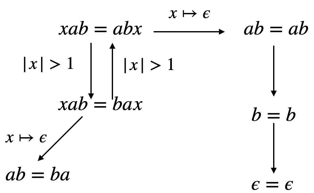
Figure 1. An example of Levi’s method applied to a simple example. This shows that $xab=abx$ is satisfiable.

The proof is standard (e.g. see [Die02]). For the sake of completeness, we illustrate this with an example and provide the crux of the proof. Figure 1 depicts an application of Nielsen’s transformation to show that $xab=abx$ is satisfiable. It is not a coincidence that this is a finite graph because the set of reachable nodes from any quadratic equation $E$ is actually finite. This finiteness property essentially can be seen as a corollary of the following two easily checked properties: (1) each rule of Nielsen transformation preserves the quadratic nature of an equation, and (2) each rule of Nielsen transformation never increases the length of an equation. This directly gives us a PSPACE algorithm: each step can be implemented in polynomial space, and the size never increases. The IFF statement in the above proposition can essentially be proven as follows. The ($\Leftarrow$) direction follows from the fact that each rule of Nielsen transformation preserves satisfiability. The ($\Rightarrow$) direction follows from the fact that, when applied to quadratic equations, each step either decreases the size of the equation, or the length of a length-minimal solution.

3.2. Handling regular constraints

Nielsen transformation easily extends to quadratic word equations with regular constraints (e.g. see [DR99]).

Recall that we are given a finite set $S=\{x_{1}\in\mathcal{L}(\mathcal{A}^{1}),\ldots,x_{n}\in\mathcal{L}(\mathcal{A}^{n})\}$ of regular constraints. We assume that the automata $\mathcal{A}^{1},\ldots,\mathcal{A}^{n}$ have disjoint state-space. This sequence $x_{1},\ldots,x_{n}$ might contain repetition of variables. Instead of allowing multiple regular constraints per variable $x$, we will assign one monoid element over boolean matrices for each variable $x$ in the following way. Suppose $\mathcal{A}^{i}$ has $r_{i}$ states, and we let $r=\sum_{i=1}^{n}r_{i}$. Let $\mathcal{A}$ be the automaton with $r$ states obtained by taking the union of $\mathcal{A}^{1},\ldots,\mathcal{A}^{n}$. Let $\mathbb{B}$ be the usual boolean algebra with two elements $0,1$. For any given word $w\in A^{*}$, we can construct the characteristic matrix $M=(m_{i,j})\in\mathbb{B}^{r\times r}$ (indexed by the states of $\mathcal{A}$ without loss of generality) as follows: for any pair $i,j$ of states, $m_{i,j}=1$ iff $w\in\mathcal{L}(\mathcal{A}_{i,j})$. Therefore, we can assign a monoid element to each variable $x$ in the following way. Take the subsequence $\mathcal{B}^{1},\ldots,\mathcal{B}^{m}$ of $\mathcal{A}^{1},\ldots,\mathcal{A}^{n}$, for which there is a regular constraint $x\in\mathcal{L}(\mathcal{B}^{i})$. Suppose $(q_{0}^{1},F^{1}),\ldots,(q_{0}^{m},F^{m})$ are the pairs of initial state and set of final states of $\mathcal{B}^{1},\ldots,\mathcal{B}^{m}$. Then, there exist a homomorphism $\phi:A^{*}\to\mathbb{B}^{r\times r}$, such that

$$w\in\bigcap_{i=1}^{m}\mathcal{L}(\mathcal{B}^{i})\quad\text{iff}\quad\forall i\in\{1,\ldots,m\}:\bigvee_{q_{F}\in F^{i}}\phi(w)[q_{0}^{i},q_{F}]=1.$$

Note that the term homomorphism here is justified since $\mathbb{B}^{r\times r}$ is a monoid with the boolean matrix multiplication operator. In the following, we will always restrict ourselves to the submonoid of $\mathbb{B}^{r\times r}$ containing only realisable characteristic matrices, i.e., those matrices $M=\phi(w)$, for some $w\in A^{*}$. Note that checking whether a boolean matrix is realisable is PSPACE-complete since it is equivalent to checking emptiness of intersection of automata [Koz77].

Our rewriting relation $\Rightarrow$ now works over a pair $(E,f)$ consisting of a word equation $E$ and a function mapping each variable $x$ in $E$ to a monoid element $M\in\mathbb{B}^{r\times r}$. Let $E$ be an equation of the form $\alpha w_{1}=\beta w_{2}$ with $w_{1},w_{2}\in(A\cup{V})^{*}$ and $\alpha,\beta\in A\cup{V}$. We now define $(E,f)\Rightarrow(E^{\prime},f^{\prime})$ by extending the previous definition of $\Rightarrow$ without regular constraints. More precisely, $(E,f)\Rightarrow(E^{\prime},f^{\prime})$ iff $E\Rightarrow E^{\prime}$ and additionally do the following:

• Rules for erasing an empty prefix variable $\alpha$. When applied, ensure that $\phi(\epsilon)=f(\alpha)$. Without loss of generality, we may assume that all our automata have no $\epsilon$-transitions, in which case $f(\alpha)$ is the identity matrix. We define $f^{\prime}$ as the restriction of $f$ to ${V}\setminus\{\alpha\}$.

• Rules for removing a nonempty prefix. For (P1), we set $f^{\prime}$ to be the restriction of $f$ to ${V}\setminus\{\alpha\}$. For (P2)–(P4), assume that $E^{\prime}$ is $w_{1}[\alpha\beta/\beta]=\beta(w_{2}[\alpha\beta/\beta])$; the other case is symmetric. We nondeterministically guess a monoid element $M_{\beta^{\prime}}$. If $\alpha\in A$, we check that $f(\beta)=\phi(\alpha)\cdot M_{\beta^{\prime}}$. If $\alpha\in{V}$, we make sure that $f(\beta)=f(\alpha)\cdot M_{\beta^{\prime}}$. Note that both of these checks can be done in polynomial time. We set $f^{\prime}$ to be the same function $f$, but differs only on $\beta$: $f^{\prime}(\beta)=M_{\beta^{\prime}}$.

We now state the main property of the above algorithm. To this end, a function $f:{V}\to\mathbb{B}^{r\times r}$ is said to be consistent with the set $S$ of regular constraints if, whenever $(x\in\mathcal{L}(\mathcal{B}))\in S$ where $\mathcal{B}$ has initial state (resp. set of final states) $p$ (resp. $F$), it is the case that $\bigvee_{q\in F}M[p,q]=1$, where $M:=f(x)$.

Proposition .

$(E,S)$ is solvable iff there exists $f:{V}\to\mathbb{B}^{r\times r}$ consistent with $S$ such that $(E,f)\Rightarrow^{*}(\epsilon=\epsilon,\emptyset)$, where $\emptyset$ denotes the function with the empty domain. Furthermore, checking if $(E,S)$ is solvable is in PSPACE.

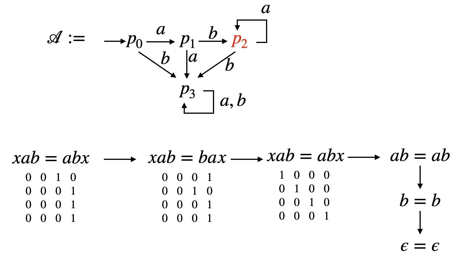
Figure 2. Building on Example from Figure 1, we add the regular constraint $x\in aba^{*}$ given by automaton $\mathcal{A}$. The automaton is quite large, but we show only the path from $(E,f)$ with consistent $f$ to $(\epsilon=\epsilon,\emptyset)$. Note that $f$ can be realized by $w=ab$.

See Figure 2 for an example. Note that the above algorithm is a nondeterministic polynomial-space algorithm (because of the guessing of $f$ in the above proposition, and also the relation $\Rightarrow$), which still gives us a PSPACE algorithm because of the standard Savitch’s Theorem that PSPACE = NPSPACE [Sip97].

3.3. Generating all solutions using Nielsen transformation

One result that we will need in this paper is that Nielsen transformation is able to generate all solutions of quadratic word equations with regular constraints. To clarify this, we extend the definition of $\Rightarrow$ so that each configuration $E$ or $(E,f)$ in the graph of $\Rightarrow$ is also annotated by an assignment ${\sigma}$ of the variables in $E$ to concrete strings. We write $E_{1}[{\sigma}_{1}]\Rightarrow E_{2}[{\sigma}_{2}]$ if $E_{1}\Rightarrow E_{2}$ and ${\sigma}_{2}$ is the modification from ${\sigma}_{1}$ according to the operation used to obtain $E_{2}$ from $E_{1}$. Observe that the domain of ${\sigma}_{2}$ is a subset of the domain of ${\sigma}_{1}$; in fact, some rules (e.g., erasing an empty prefix variable) could remove a variable in the prefix in $E_{1}$ from ${\sigma}_{1}$. The following example illustrates how $\Rightarrow$ works with this extra annotated assignment. Suppose that ${\sigma}_{1}(x)=ab$ and ${\sigma}_{1}(y)=abab$ and $E_{1}:=xy=yx$ and $E_{2}$ is obtained from $E_{1}$ using rule (P4), i.e., substitute $xy$ for $y$. In this case, ${\sigma}_{2}(x)={\sigma}_{2}(y)={\sigma}_{1}(x)=ab$. Observe that $E_{2}[{\sigma}_{2}]\Rightarrow E_{3}[{\sigma}_{3}]\Rightarrow E_{4}[{\sigma}_{4}]$, where $E_{3}:=E_{2}$, ${\sigma}_{3}(x)=ab$, ${\sigma}_{3}(y)=\epsilon$, $E_{4}:=x=x$, and ${\sigma}_{4}(x)=ab$. The definition for the case with regular constraints is identical.

Proposition .

$(E,f)[{\sigma}]\to^{*}(\epsilon=\epsilon,\emptyset)[{\sigma}^{\prime}]$ where ${\sigma}^{\prime}$ has the empty domain iff ${\sigma}$ is a solution of $(E,f)$.

This proposition immediately follows from the proof of correctness of Nielsen transformation for quadratic word equations (cf. [Die02]).

3.4. Length abstractions and semilinearity

Below we tacitly assume an implicit ordering of the set of variables ${V}=\{x_{1},\ldots,x_{k}\}$ — which ordering is immaterial, so long as one is fixed. Given a quadratic word equation $E$ with constants $A$ and variables ${V}=\{x_{1},\ldots,x_{k}\}$, its length abstraction is defined as follows

$$\text{{Len}}(E)=\{(|{\sigma}(x_{1})|,\ldots,|{\sigma}(x_{k})|):\text{${\sigma}$ is a solution to $E$}\},$$

namely the set of tuples of numbers corresponding to lengths of solutions to $E$.

Example .

Consider the quadratic equation $E:=\ xaby=yz$, where ${V}=\{x,y,z\}$ and $A$ contains at least two letters $a$ and $b$. We will show that its length abstraction $\text{{Len}}(E)$ can be captured by the Presburger formula $|z|=|x|+2$. Observe that each $(n_{x},n_{y},n_{z})\in\text{{Len}}(E)$ must satisfy $n_{z}=n_{x}+2$ by a length argument on $E$. Conversely, we will show that each triple $(n_{x},n_{y},n_{z})\in\mathbb{N}^{3}$ satisfying $n_{z}=n_{x}+2$ must be in $\text{{Len}}(E)$. To this end, we will define a solution ${\sigma}$ to $E$ such that $(|{\sigma}(x)|,|{\sigma}(y)|,|{\sigma}(z)|)=(n_{x},n_{y},n_{z})$. Consider ${\sigma}(x)=a^{n_{x}}$. Then, for some $q\in\mathbb{N}$ and $r\in[n_{x}+1]$, we have $n_{y}=q(n_{x}+2)+r$. Let $w$ be a prefix of ${\sigma}(x)ab$ of length $r$. Therefore, for some $v$, we have $wv={\sigma}(x)ab$. Define ${\sigma}(y)=({\sigma}(x)ab)^{q}w$. We then have ${\sigma}(x)ab{\sigma}(y)={\sigma}(y)vw$. Thus, setting ${\sigma}(z)=vw$ gives us a satisfying assignment for $E$ which satisfies the desired length constraint. ∎

However, it turns out that Presburger Arithmetic is not sufficient for capturing length abstractions of quadratic word equations.

Theorem .

There is a quadratic word equation whose length abstraction is not Presburger-definable.

To this end, we show that the length abstraction of $xaby=yabx$, where $a,b\in A$ and $x,y\in{V}$, is not Presburger definable.

Lemma .

The length abstraction $\text{{Len}}(xaby=yabx)$ coincides with tuples $(|x|,|y|)$ of numbers satisfying the expression $\varphi(|x|,|y|)$ defined as:

$$|x|=|y| \vee (|x|=0\wedge|y|\equiv 0\pmod{2})\vee(|y|=0\wedge|x|\equiv 0\pmod{2})$$

$$\vee (|x|,|y|>0\wedge\gcd(|x|+2,|y|+2)>1)$$

Observe that this would imply non-Presburger-definability: for otherwise, since the first three disjuncts are Presburger-definable, the last disjunct would also be Presburger-definable, which is not the case since the property that two numbers are relatively prime is not Presburger-definable. Let us prove this lemma. Let $S=\text{{Len}}(xaby=yabx)$. We first show that given any numbers $n_{x},n_{y}$ satisfying $\varphi(n_{x},n_{y})$, there are solutions ${\sigma}$ to $xaby=yabx$ with $|{\sigma}(x)|=n_{x}$ and $|{\sigma}(y)|=n_{y}$. If they satisfy the first disjunct in $\varphi$ (i.e., $n_{x}=n_{y}$), then set ${\sigma}(x)={\sigma}(y)$ to an arbitrary word $w\in A^{n_{x}}$. If they satisfy the second disjunct, then $aby=yab$ and so set ${\sigma}(x)=\epsilon$ and ${\sigma}(y)\in(ab)^{*}$. The same goes with the third disjunct, symmetrically. For the fourth disjunct (assuming the first three disjuncts are false), let $d=\gcd(n_{x}+2,n_{y}+2)$. Define ${\sigma}(x),{\sigma}(y)\in(a^{d-1}b)^{*}(a^{d-2})$ so that $|{\sigma}(\alpha)|=n_{\alpha}$ for $\alpha\in{V}$. It follows that ${\sigma}(x)ab{\sigma}(y)={\sigma}(y)ab{\sigma}(x)$.

We now prove the converse. So, we are given a solution ${\sigma}$ to $xaby=yabx$ and let $u:={\sigma}(x)$, $v:={\sigma}(y)$. Assume to the contrary that $\varphi(|u|,|v|)$ is false and that $u$ and $v$ are the shortest such solutions. We have several cases to consider:

• $u=v$. Then, $|u|=|v|$, contradicting that $\varphi(|u|,|v|)$ is false.

• $u=\epsilon$. Then, $abv=vab$ and so $v\in(ab)^{*}$, which implies that $|v|\equiv 0\pmod{2}$. Contradicting that $\varphi(|u|,|v|)$ is false.

• $v=\epsilon$. Same as previous item and that $|u|\equiv 0\pmod{2}$.

• $|u|>|v|>0$. Since $\varphi(|u|,|v|)$ is false, we have $\gcd(|u|+2,|v|+2)=1$. It cannot be the case that $|u|=|v|+1$ since then, comparing prefixes of $uabv=vabu$, the letter at position $|u|+2$ would be $b$ on l.h.s. and $a$ on r.h.s., which is a contradiction. Therefore $|u|\geq|v|+2$. Let $u^{\prime}=u[|v|+3,|u|]$, i.e., $u$ but with its prefix of length $|v|+2$ removed. By Nielsen transformation, we have $u^{\prime}abv=vabu^{\prime}$. It cannot be the case that $u^{\prime}=\epsilon$; for, otherwise, $abv=vab$ implies $v\in(ab)^{*}$ and so $u=vab$, implying that 2 divides both $|u|+2$ and $|v|+2$, contradicting that $\gcd(|u|+2,|v|+2)=1$. Therefore, $|u^{\prime}|>0$. Since $\gcd(|u^{\prime}|+2,|v|+2)=\gcd(|u|+2,|v|+2)=1$, we have a shorter solution to $xaby=yabx$, contradicting minimality.

• $|v|>|u|>0$. Same as previous item.

4. Reduction to Counter Systems

In this section, we will provide an algorithm for computing a counter system from $(E,S)$, where $E$ is a quadratic word equation and $S$ is a set of regular constraints. We will first describe this algorithm for the case without regular constraints, after which we show the extension to the case with regular constraints.

Given the quadratic word equation $E$, we show how to compute a counter system $\mathcal{C}(E)=(X,Q,\Delta)$ such that the following theorem holds.

Theorem .

The length abstraction of $E$ coincides with

$${\{v\in\mathbb{N}^{|{V}|}\mid(E,v)\in{\rm Phys.~{}Rev.~{}E}_{\mathcal{C}(E)}^{*}(\{\epsilon=\epsilon\}\times\mathbb{N}^{|{V}|})\}}$$

Before defining $\mathcal{C}(E)$, we define some notation. Define the following formulas:

• $\text{{ID}}(\bar{x},\bar{x}^{\prime}):=\bigwedge_{x\in\bar{x}}x^{\prime}=x$

• $\text{{SUB}}_{y,z}(\bar{x},\bar{x}^{\prime}):=\text{{{$0<$}}}z\leq y\wedge y^{\prime}=y-z\wedge\bigwedge_{x\in\bar{x},x\neq y}x^{\prime}=x$

• $\text{{DEC}}_{y}(\bar{x},\bar{x}^{\prime}):=y>0\wedge y^{\prime}=y-1\wedge\bigwedge_{x\in\bar{x},x\neq y}x^{\prime}=x$

Note that the $\neq$ symbol in the guard of $\bigwedge$ denotes syntactic equality (i.e. not equality in Presburger Arithmetic). We omit mention of the free variables $\bar{x}$ and $\bar{x}^{\prime}$ when they are clear from the context.

We now define the counter system. Given a quadratic word equation $E$ with constants $A$ and variables ${V}$, we define a counter system $\mathcal{C}(E)=(X,Q,\Delta)$ as follows. The counters $X$ will be precisely all variables that appear in $E$, i.e., $X:={V}$. The control states are precisely all equations $E^{\prime}$ that can be rewritten from $E$ using Nielsen transformation, i.e., $Q:=\{E^{\prime}:E\Rightarrow^{*}E^{\prime}\}$. The set $Q$ is finite (at most exponential in $|E|$) as per our discussion in the previous section.

We now define the transition relation $\Delta$. We use $\bar{x}$ to enumerate ${V}$ in some order. Given $E_{1}\Rightarrow E_{2}$ with $E_{1},E_{2}\in Q$, we then add the transition $(E_{1},\Phi(\bar{x},\bar{x}^{\prime}),E_{2})$, where $\Phi$ is defined as follows:

(r1):

If $E_{1}\Rightarrow E_{2}$ applies a rule for erasing an empty prefix variable $y\in\bar{x}$, then $\Phi:=y=0\wedge\text{{ID}}$.

(r2):

If $E_{1}\Rightarrow E_{2}$ applies a rule for removing a nonempty prefix:

• If (P1) is applied, then $\Phi=\text{{ID}}$.

• If (P2) is applied, then $\Phi=\text{{DEC}}_{\beta}$.

• If (P3) is applied, then $\Phi=\text{{DEC}}_{\alpha}$.

• If (P4) is applied and $\alpha\preceq\beta$, then $\Phi=\text{{SUB}}_{\beta,\alpha}$. If $\beta\preceq\alpha$, then $\Phi=\text{{SUB}}_{\alpha,\beta}$.

Lemma .

The counter system $\mathcal{C}(E)$ terminates from every configuration $(E_{0},\text{\rm v}_{0})$.

Proof.

By checking each transition rule defined for $\mathcal{C}(E)$, it is easy to verify that if $(E_{1},\text{\rm v}_{1})\to(E_{2},\text{\rm v}_{2})$, then $|E_{1}|\leq|E_{2}|$ and $\text{\rm v}_{1}\preceq\text{\rm v}_{2}$. In addition, if $\text{\rm v}_{1}=\text{\rm v}_{2}$, then $|E_{1}|<|E_{2}|$. Indeed, $\text{\rm v}_{1}=\text{\rm v}_{2}$ could hold only in the case of applying (r1) or (r2,P1); the other rules would guarantee that $\text{\rm v}_{2}\prec\text{\rm v}_{1}$ because of the nonzero assumption for the decrementing counter. It is clear that (r1) and (r2,P1) would ensure that $|E_{2}|<|E_{1}|$. This guarantees that it takes at most $|E_{0}|+\|\text{\rm v}_{0}\|$ steps before $\mathcal{C}(E)$ terminates from $(E_{0},\text{\rm v}_{0})$, where $\|\text{\rm v}\|$ denotes the sum of all the components in v. This completes the proof of the lemma. ∎

The proof of Theorem 4 immediately follows from Proposition 3.3 that Nielsen transformation generates all solutions. We illustrate how such a counter system is constructed on the simple example $xy=yz$ in Figure 3.

Figure 3. A depiction of parts of $\mathcal{C}(xy=yz)$.

Extension to the case with regular constraints:

In this extension, we will only need to assert that initial counter values belong to the length abstractions of the regular constraints, which are effectively semilinear due to Parikh’s Theorem [Par66]. Given a quadratic word equation $E$ with a set $S$ of regular constraints, we define the counter system $\mathcal{C}(E,S)=(X,Q,\Delta)$ as follows. Let $\mathcal{C}(E)=(X_{1},Q_{1},\Delta_{1})$ be the counter system from the previous paragraph, obtained by ignoring the regular constraints. We define $X=X_{1}$. Let $Q$ be the finite set of all configurations reachable from some $(E,f)$ where $f$ is a monoid element consistent with $S$, i.e., $Q=\{(E^{\prime},f^{\prime}):(E,f)\Rightarrow^{*}(E^{\prime},f^{\prime})\}$. Given $(E_{1},f_{1})\Rightarrow(E_{2},f_{2})$, we add the transition $((E_{1},f_{2}),\Phi(\bar{x},\bar{x}^{\prime}),(E_{2},f_{2}))$ to $\mathcal{C}(E,S)$ if $(E_{1},\Phi(\bar{x},\bar{x}^{\prime}),E_{2})$ was added to $\Delta_{1}$ by $E_{1}\Rightarrow E_{2}$. The following theorem generalises Theorem 4 by asserting that the initial counter values belong to the length abstractions of a monoid element consistent with the regular constraints.

Theorem .

The length abstraction of $(E,S)$ coincides with

$$\bigcup_{f}\left({\{v\in\mathbb{N}^{{V}}\mid((E,f),v)\in{\rm Phys.~{}Rev.~{}E}_{\mathcal{C}(E,S)}^{*}(\{(\epsilon=\epsilon,\emptyset)\}\times\mathbb{N}^{{V}})\}}\cap\text{{Len}}_{\bar{x}}(\phi^{-1}(f))\right),$$

where $f$ ranges over partial functions mapping ${V}$ to $\mathbb{B}^{r\times r}$ that are consistent with $S$, and $\text{{Len}}_{\bar{x}}(\phi^{-1}(f))$ is a shorthand for $\{v\in\mathbb{N}^{{V}}\mid v(x)\in\text{{Len}}(\phi^{-1}(f(x))),\text{{{for all $x\in{V}$}}}\}$.

As for the case without regular constraints, the proof of Theorem 4 immediately follows from Proposition 3.3 that Nielsen transformation generates all solutions. As previously mentioned, $\text{{Len}}_{\bar{x}}(\phi^{-1}(f))$ is semilinear by Parikh’s Theorem [Par66]. Unlike Theorem 4, however, Theorem 4 is not achieved by a polynomial-time reduction for two reasons. Firstly, there could be exponentially many functions $f$ that are consistent with $S$, and that checking this consistency is PSPACE-complete. Secondly, the size of the NFA for $\phi^{-1}(f(x))$ is exponential in the total number of states in automata in the set $S$ of regular constraints. It turns out that this reduction can be made to run in polynomial-space. Enumerating the candidate function $f$ can be done in polynomial space, as previously remarked.

Lemma .

There is a polynomial-space algorithm which enumerates linear sets corresponding to $\text{{Len}}_{\bar{x}}(\phi^{-1}(f))$.

This lemma essentially follows from the proof of the result of Kopczynski and To [KT10] that one can compute a union of $n^{k^{O(1)}}$ linear sets each with at most $k$ periods with numbers represented in unary (with time complexity $n^{k^{O(1)}}$, and polynomial space) representing the Parikh image of an NFA with $k$ letters in the alphabet. This result can be easily adapted to show that, given NFAs $\mathcal{A}_{1},\ldots,\mathcal{A}_{n}$, one can enumerate in polynomial space a union of exponentially many linear sets of polynomial size (with at most $k$ periods and numbers represented in binary) representing the Parikh image of $\mathcal{L}(\mathcal{A}_{1})\cap\cdots\cap\mathcal{L}(\mathcal{A}_{n})$. Since $\phi^{-1}(f(x))$ can be represented by an intersection of polynomially many NFA, Lemma 4 immediately follows.

5. Decidability via Linear Arithmetic with Divisibility

5.1. Accelerating a 1-variable-reducing cycle

Consider a counter system $\mathcal{C}=(X,Q,\Delta)$ with $Q=\{q_{0},\ldots,q_{n-1}\}$, such that for some $y\in X$ the transition relation $\Delta$ consists of precisely the following transition $(q_{i},\Phi_{i},q_{i+1\pmod{n}})$, for each $i\in[n-1]$, and each $\Phi_{i}$ is either $\text{{SUB}}_{y,z}$ (with $z$ a variable distinct from $y$) or $\text{{DEC}}_{y}$. Such a counter system is said to be a 1-variable-reducing cycle.

Lemma .

There exists a polynomial-time algorithm which given a 1-variable-reducing cycle $\mathcal{C}=(X,Q,\Delta)$ and two states $p,q\in Q$ computes a formula $\varphi_{p,q}(\bar{x},\bar{x}^{\prime})$ in existential Presburger arithmetic with divisibility such that $(p,\text{\rm v})\to_{\mathcal{C}}^{*}(q,\text{\rm w})$ iff $\varphi_{p,q}(\text{\rm v},\text{\rm w})$ is satisfiable.

This lemma can be seen as a special case of the acceleration lemma for flat parametric counter automata [BIL09] (where all variables other than $y$ are treated as parameters). However, its proof is in fact quite simple. Without loss of generality, we assume that $q=q_{0}$ and $p=q_{i}$, for some $i\in[0,n-1]$. Any path $(q_{0},\text{\rm v})\to_{\mathcal{C}}^{*}(q_{i},\text{\rm w})$ can be decomposed into the cycle $(q_{0},\text{\rm v})\to^{*}(q_{0},\text{\rm v}^{\prime})$ and the simple path $(q_{0},\text{\rm w}_{0})\to\cdots\to(q_{i},\text{\rm w}_{i})$ of length $i$. Therefore, the reachability relation $(q_{0},\text{\rm x})\to_{\mathcal{C}}^{*}(q_{i},\text{\rm y})$ can be expressed as

$$\exists\text{\rm z}_{0},\cdots,\text{\rm z}_{i-1}:\varphi_{q_{0},q_{0}}(\text{\rm x},\text{\rm z}_{0})\wedge\Phi_{0}(\text{\rm z}_{0},\text{\rm z}_{1})\wedge\cdots\wedge\Phi_{i-1}(\text{\rm z}_{i-1},\text{\rm y}).$$

Thus, it suffices to show that $\varphi_{q_{0},q_{0}}(\text{\rm x},\text{\rm x}^{\prime})$ is expressible in PAD. Consider a linear expression $M=a_{0}+\sum_{x\in X\setminus{\{y\}}}a_{x}x$, where $a_{0}$ is the number of instructions $i$ in the cycle such that $\Phi_{i}=\text{{DEC}}_{y}$ and $a_{x}$ is the number of instructions $i$ such that $\Phi_{i}=\text{{SUB}}_{y,x}$. Each time around the cycle, $y$ decreases by $M$. Thus, for some $n\in\mathbb{N}$ we have $y^{\prime}=y-nM$, or equivalently

$$nM=y-y^{\prime}$$

The formula $\varphi_{q_{0},q_{0}}$ can be defined as follows:

$$\varphi_{q_{0},q_{0}}:=\ M\mid(y-y^{\prime})\wedge y^{\prime}\leq y\wedge\bigwedge_{x\in X\setminus\{y\}}x^{\prime}=x.$$

5.2. An extension to flat control structures

The following generalisation to flat control structures is an easy corollary of Lemma 5.1.

Theorem .

There exists an NP algorithm with a PAD oracle for the following problem: given a flat Presburger counter system $\mathcal{C}=(X,Q,\Delta)$, each of whose simple cycle is 1-variable-reducing two states $p,q\in Q$, and an existential Presburger formula $\psi(\bar{x},\bar{y})$, decide if $(p,\text{\rm v})\to_{\mathcal{C}}^{*}(q,\text{\rm w})$ for some $\text{\rm v},\text{\rm w}$ such that $\psi(\text{\rm v},\text{\rm w})$ is a valid Presburger formula. That is, the problem is solvable in time NEXP.

Proof.

Consider the control graph $G=(V,E)$ of $\mathcal{C}$. To witness $(p,\text{\rm v})\to_{\mathcal{C}}^{*}(q,\text{\rm w})$ for some $\text{\rm v},\text{\rm w}$ such that $\psi(\text{\rm v},\text{\rm w})$ is true, it is sufficient and necessary that the execution of $\mathcal{C}$ corresponds to a skeleton of $G$ from $p$ to $q$ with a specific entry point (together with a specific incoming transition) and a specific exit point (together with a specific outgoing transition) for each cycle. Namely, this path can be described as:

$$\pi:=v_{0}\to_{E}^{*}v_{0}^{\prime}\to_{e_{1}}v_{1}\to_{E}^{*}v_{1}^{\prime}\to_{e_{2}}\cdots\to_{e_{k}}v_{k}\to_{E}^{*}v_{k}^{\prime}$$

where

• $v_{0}=p$ and $v_{k}^{\prime}=q$

• $v_{i}$ and $v_{i}^{\prime}$ belong to the same SCC in $G$

• $v_{i}^{\prime}$ and $v_{i+1}$ belong to different SCCs in $G$.

In other words, each $v_{i}$ (resp. $v_{i}^{\prime}$) describes the entry (resp. exit) node for the $i$th SCC that is used in this path. Our algorithm first guesses this path $\pi$. We construct the formula $\varphi_{v_{i},v_{i}^{\prime}}(\bar{x}_{i},\bar{x}_{i}^{\prime})$ by means of Lemma 5.1. We then only need to use a PAD solver to check satisfiability for the formula

$$\Phi:=\left(\bigwedge_{i=0}^{k}\varphi_{v_{i},v_{i}^{\prime}}(\bar{x}_{i},\bar{x}_{i}^{\prime})\right)\wedge\left(\bigwedge_{i=1}^{k}\theta_{i}(\bar{x}_{i-1}^{\prime},\bar{x}_{i})\right)\wedge\psi(\bar{x}_{1},\bar{x}_{k}^{\prime}),$$

where $\theta_{i}$ applies the transition $e_{i}$ to $\bar{x}_{i-1}^{\prime}$ to obtain $\bar{x}_{i}$. That is, we have $e_{i}=(v_{i}^{\prime},\theta_{i}(\bar{x},\bar{x}^{\prime}),v_{i})$. Altogether, we obtain an NP algorithm with an access to PAD oracle for the problem. The NEXP upper bound [LOW15] for PAD gives us also an NEXP upper bound for our problem. ∎

Remark .

Note that the reduction from system of word equations to a single word equation that we remark in Section 2 may preserve flatness, but that is not necessarily the case. The positive example where flatness is preserved is given in Section 2, but an example where flatness is not preserved is $xy=yz\wedge z=x$.

5.3. Application to word equations with length constraints

Theorem 5.2 gives rise to a simple and sound (but not complete) technique for solving quadratic word equations with length constraints: given a quadratic word equation $(E,S)$ with regular constraints, if the counter system $\mathcal{C}(E,S)$ is flat, each of whose simple cycle is 1-variable-reducing with unary Presburger guards, then apply the decision procedure from Theorem 5.2. In this section, we show completeness of this method for the class of regular-oriented word equations recently defined in [DMN17], which can be extended with regular constraints given as 1-weak NFA [BRS12]. A word equation is regular if each variable $x\in{V}$ occurs at most once on each side of the equation. Observe that $xy=yx$ is regular, but $xxyy=zz$ is not. It is easy to see that a regular word equation is quadratic. A word equation $L=R$ is said to be oriented if there is a total ordering $<$ on ${V}$ such that the occurrences of variables on each side of the equation preserve $<$, i.e., if $w=L$ or $w=R$ and $w=w_{1}\alpha w_{2}\beta w_{3}$ for some $w_{1},w_{2},w_{3}\in(A\cup{V})^{*}$ and $\alpha,\beta\in{V}$, then $\alpha<\beta$. Observe that $xy=yz$ (i.e. that $x$ and $z$ are conjugates) is oriented, but $xy=yx$ is not oriented. It was shown in [DMN17] that the satisfiability for regular-oriented word equations is NP-hard. We show satisfiability for this class with length constraints is decidable.

Theorem .

The satisfiability problem of regular-oriented word equations with length constraints is decidable in nondeterministic exponential time. In fact, it is solvable in NP with PAD oracles.

This decidability (in fact, an NP upper bound) for the strictly regular-ordered subcase, in which each variable occurs precisely once on each side, was proven in [D⁺18]. For this subcase, it was shown that Presburger Arithmetic is sufficient, but the decidability for the general class of regular-oriented word equations with length constraints remained open.

We start with a simple lemma that $\Rightarrow$ preserves regular-orientedness.

Lemma .

If $E\Rightarrow E^{\prime}$ and $E$ is regular-oriented, then $E^{\prime}$ is also regular-oriented.

Proof.

It is easy to see each rewriting rule preserves regularity. Now, because $E^{\prime}$ is regular, to show that $E^{\prime}:=L=R$ is also oriented it is sufficient and necessary to show that there are no two variables $x,y$ such that $x$ occurs before $y$ in $L$, but $y$ occurs before $x$ in $R$. All rewriting rules except for (P2)–(P4) are easily seen to preserve orientedness. Let us write $E:=\alpha w_{1}=\beta w_{2}$ with $\alpha\neq\beta$, and assume $E^{\prime}=E[\alpha\beta/\beta]$; the case of $E^{\prime}=E[\beta\alpha/\alpha]$ is symmetric. So, $\beta$ is some variable $y$. If $\beta$ does not occur in $w_{1}$, then $L=w_{1}$ and $R=\beta w_{2}$ and that $E$ is oriented implies that $E^{\prime}$ is oriented. So assume that $\beta$ appears in $w_{1}$, say, $w_{1}=u\beta v$. Then, $R=\beta w_{2}$ and $L=u\alpha\beta v$. Thus, if $\alpha\in A$, $E^{\prime}$ is oriented because we can use the same variable ordering that witnesses that $E$ is oriented. So, assume $\alpha\in{V}$. It suffices to show that $\alpha$ occurs at most once in $E$. For, if $\alpha$ also occurs on the other side of the equation $E$ (i.e. in $w_{2}$), $\alpha$ precedes $\beta$ on l.h.s. of $E$, while $\beta$ precedes $\alpha$ on r.h.s. of $E$, which would show that $E$ is not oriented. ∎

Next, we show a bound on the lengths of cycles and paths of the counter system associated with a regular-oriented word equation.

Lemma .

Given a regular-oriented word equation $E$, the counter system $\mathcal{C}(E)$ is flat, where each simple cycle is 1-variable-reducing. Moreover, the length of each simple cycle (resp. path) in the control structure of $\mathcal{C}(E)$ is $O(|E|)$ (resp. $O(|E|^{2})$).

As an example, the reader can confirm the flatness of $\mathcal{C}(xy=yz)$ by studying the counter system in Figure 3.

Proof.

We now show Lemma 5.3. Let $E:=L=R$. We first analyze the shape of a simple cycle, from which we will infer most of the properties claimed in Lemma 5.3. Given a simple cycle $E_{0}\Rightarrow E_{1}\Rightarrow\cdots\Rightarrow E_{n}$ with $n>0$ (i.e. $E_{0}=E_{n}$ and $E_{i}\neq E_{j}$ for all $0\leq i<j<n$), it has to be the case that each rewriting in this cycle applies one of the (P2)–(P4) rules since the other rules reduce the size of the equation. We have $|E_{0}|=|E_{1}|=\cdots=|E_{n}|$. Let $E_{i}:=L_{i}=R_{i}$ with $L_{i}=\alpha_{i}w_{i}$ and $R_{i}=\beta_{i}w_{i}^{\prime}$. Let us assume that $E_{1}$ be $w_{0}[\alpha_{0}\beta_{0}/\beta_{0}]=\beta_{0}w_{0}^{\prime}[\alpha_{0}\beta_{0}/\beta_{0}]$; the case with $E_{1}$ be $\alpha_{0}w_{0}[\beta_{0}\alpha_{0}/\alpha_{0}]=w_{0}^{\prime}[\beta_{0}\alpha_{0}/\alpha_{0}]$ will be easily seen to be symmetric. This assumption implies that $\beta_{0}$ is a variable $y$, and that $L_{0}=uyv$ for some words $u,v\in(A\cup{V})^{*}$ (for, otherwise, $|E_{1}|<|E_{0}|$ because of regularity of $E$). Furthermore, it follows that, for each $i\in[n-1]$, $E_{i+1}$ is $w_{i}[\alpha_{i}y/{{y}}]=yw_{i}^{\prime}$ and $\beta_{i}=y$, i.e., the counter system $\mathcal{C}(E)$ applies either $\text{{SUB}}_{y,x}$ (in the case when $x=\alpha_{i}$) or $\text{{DEC}}_{y}$ (in the case when $\alpha_{i}\in A$). For, otherwise, taking a minimal $i\in[1,n-1]$ with $E_{i+1}$ being $\alpha_{i}w_{i}[y\alpha_{i}/\alpha_{i}]=w_{i}^{\prime}[y\alpha_{i}/\alpha_{i}]$ for some variable $x=\alpha_{i}$ shows that $E_{i}$ is of the form $x...y...=y...x...$ (since $|E_{i+1}|=|E_{i}|$) contradicting that $E_{i}$ is oriented. This shows that this simple cycle is 1-variable-reducing. Consequently, we have

• $R_{i}=R_{j}$ for all $i,j$, and

• $L_{i}=\mathrm{cyc}^{i}(u)yv$ for all $i\in[n]$

The shape of the equations in this simple cycle guarantees also that any edge out of this simple cycle reduces the length of the equation, which guarantees that each of the nodes $E_{1},\ldots,E_{n}$ only has this as the unique cycle. Finally, the length of the cycle is at most $|L_{0}|-1\leq|L|-1$. Since this simple cycle is taken arbitrarily, it follows that the structure of $\mathcal{C}(E)$ is flat, each of whose simple cycle is 1-variable-reducing and is of length at most $N=\max\{|L|,|R|\}-1$.

Consider the signature (i.e. dag of SCCs) of the control structure $\mathcal{C}(E)$; see Preliminaries for the definition of “signature”. In this dag, each edge from one SCC to the next is size-reducing. Therefore, the maximal length of a path in this dag is $|E|$. Therefore, since the maximal path of each SCC is $N$ (from the above analysis), the maximal length of a simple path in the control structure is at most $N^{2}$. ∎

This Lemma implies Theorem 5.3 for the following reason. We nondeterministically guess one skeleton of $\mathcal{C}(E)$ from initial node $E:=L=R$ to $\epsilon=\epsilon$. By Lemma 5.3, this is of polynomial-size and so we can apply Theorem 5.2 to obtain a nondeterministic polynomial-time algorithm with a PAD oracle.

Remark .

Note that the same example in Remark 5.2 shows that the reduction from a system of word equations — where each equation is regular-oriented — to a single word equation does not preserve regular-orientedness. It might be possible to extend the notion of regular-orientedness appropriately to a system of word equations (similar to the extension of the definition of regular word equations to a regular system of word equations given in [DM20]). We leave this for future work.

Handling regular constraints: We now extend Theorem 5.3 with regular constraints.

Theorem .

The satisfiability problem of regular-oriented word equations with regular constraints and length constraints is solvable in nondeterministic exponential time. In fact, it is solvable in PSPACE with PAD oracles.

Let us prove this theorem. The first key lemma to prove this theorem is the following:

Lemma .

The counter system $\mathcal{C}(E,S)$ is flat, where each cycle is 1-variable-reducing. Moreover, the length of each simple cycle in the control structure of $\mathcal{C}(E,S)$ is exponential in $|E|$. The maximal length of a skeleton in the control structure of $\mathcal{C}(E,S)$ is the same as the maximal length of a skeleton in the control structure of $\mathcal{C}(E)$, which is polynomial in $|E|$.

Note that this does not immediately imply the complexity upper bound of PSPACE with PAD oracles (which we will show later below), but it does imply decidability in the same way as Lemma 5.3 implies Theorem 5.3. More precisely, we nondeterministically guess a skeleton in $\mathcal{C}(E,S)$, say, starting from $(E,f)$, where $f$ is a monoid element consistent with $S$. By Theorem 5.2, we obtain the PAD formula $\psi(\bar{x},\bar{x}^{\prime}):=\lambda_{(E,f),(\epsilon=\epsilon,\emptyset)}(\bar{x},\bar{x}^{\prime})$. If the length constraint is $\theta(\bar{x})$, following Theorem 4 and Lemma 4, our polynomial-space algorithm enumerates linear sets $\eta(\bar{x})$ representing the semilinear set $\text{{Len}}_{\bar{x}}(\phi^{-1}(f))$. We will then ask the query

$$\theta(\bar{x})\wedge\eta(\bar{x})\wedge\exists\bar{x}^{\prime}\psi(\bar{x},\bar{x}^{\prime})$$

to the PAD solver.

Proof of Lemma 5.3.

By Lemma 5.3, we know that $\mathcal{C}(E)$ is flat. So, suppose that $\mathcal{C}(E,S)$ is not flat. Therefore, we may take two different cycles $\pi,\pi^{\prime}$ both visiting some node $(E,f)$. We write $\pi:(E_{0},f_{0})\to\cdots\to(E_{n},f_{n})$, and $\pi^{\prime}:(E_{0}^{\prime},f_{0}^{\prime})\to\cdots\to(E_{m}^{\prime},f_{m}^{\prime})$, where $(E_{0},f_{0})=(E_{0}^{\prime},f_{0}^{\prime})=(E_{n},f_{n})=(E_{m}^{\prime},f_{m}^{\prime})=(E,f)$. Projecting to the first argument, it must be the case that $C=E_{0}\to\cdots\to E_{n}$ and $C^{\prime}=E_{0}^{\prime}\to\cdots\to E_{m}^{\prime}$ are the same cycle in $\mathcal{C}(E)$, repeated several times. In particular, this means that, for some counter $y$, each counter instruction in these cycles are either of the form $\text{{DEC}}_{y}$ or $\text{{SUB}}_{y,x}$. Without loss of generality, let us assume that $n\leq m$ (otherwise, we swap $\pi$ and $\pi^{\prime}$). We may assume that $\pi$ and $\pi^{\prime}$ are length-minimal. We will show that $n=m$, and that $f_{i}=f_{i}^{\prime}$ for all $i$. Since $C$ and $C^{\prime}$ are the same cycle in $\mathcal{C}(E)$, there is a unique sequence of monoid elements $M_{0},\ldots,M_{m-1}$ such that:

1. $f_{i}(y)=M_{i}\cdot f_{i+1}(y)$ for all $i\in\{0,\ldots,n-1\}$, and

2. $f_{i}^{\prime}(y)=M_{i}\cdot f_{i+1}^{\prime}(y)$ for all $i\in\{0,\ldots,m-1\}$.

This implies that

$$f_{0}(y) = \left(\prod_{i=0}^{n-1}M_{i}\right)\cdot f_{0}(y)$$

$$f_{0}(y) = \left(\prod_{i=0}^{m-1}M_{i}\right)\cdot f_{0}(y)$$

implying that both $\prod_{i=1}^{n-1}M_{i}$ and $\prod_{i=1}^{m-1}M_{i}$ are the (unique) identity matrix $I$. This implies that if $m>n$, we would have that

$$f_{n}^{\prime}(y)=\left(\prod_{i=n}^{m-1}M_{i}\right)\cdot f_{0}(y)$$

which contradicts minimality of the cycle $\pi^{\prime}$. Therefore, we have $n=m$. Since $f_{n}=f_{n}^{\prime}=f$, by the equations in (1) and (2) we have that $f_{i}=f_{i}^{\prime}$ for all $i\in\{0,\ldots,n\}$. This proof also contradicts the fact that $\pi$ and $\pi^{\prime}$ are different cycles. Therefore, $\mathcal{C}(E,S)$ is flat, and we also conclude from the above proof that each cycle is 1-variable-reducing.

Let us now analyze the length of the cycles and paths in $\mathcal{C}(E,S)$. Note that in the above argument $n$ is at most the size of the monoid $\mathbb{B}^{n\times n}$, which is exponential in $n$. Observe that taking a projection of each skeleton in $\mathcal{C}(E,S)$ to the first component (i.e. omitting the monoid elements) gives us a unique skeleton in $\mathcal{C}(E)$. The converse is of course also true: given a skeleton $\pi$ in $\mathcal{C}(E)$, there is at least one skeleton $\pi^{\prime}$ in $\mathcal{C}(E,S)$ whose projection to the first component corresponds to $\pi$. This shows that the maximal length of skeletons in $\mathcal{C}(E,S)$ coincides with the maximal length of skeletons in $\mathcal{C}(E)$. ∎

To conclude the complexity bound, it suffices to provide a polynomial-space algorithm which accelerates the exponentially-sized cycles in the control structure of $\mathcal{C}(E,S)$.

Lemma .

There is a polynomial-space algorithm which given two control states $p:=(E,f),q:=(E^{\prime},f^{\prime})$ in a cycle in $\mathcal{C}:=\mathcal{C}(E,S)$ computes a formula $\varphi_{p,q}(\bar{x},\bar{x}^{\prime})$ in PAD such that $(p,\text{\rm v})\to^{*}_{\mathcal{C}}(q,\text{\rm w})$ iff $\varphi_{p,q}(\text{\rm v},\text{\rm w})$ is satisfiable.

Proof.

Firstly, observe that checking that $p$ and $q$ are in the same cycle $\pi$ can be checked in polynomial space. The proof of this lemma is exactly the same as the proof of Lemma 5.1, but with one important difference: we store the coefficients for each variable in binary, and we find these coefficients in polynomial space.

We elaborate the details below. Assume that the cycle has length $n$ and is of the form $q_{0}\to q_{1}\to\cdots\to q_{n-1}\to q_{0}$, where $q_{0}=p$ and $q_{j}=q$ for some $j\in[n-1]$. Assume further that the $i$th transition is $(q_{i},\Phi_{i},q_{i+1\pmod{n}})$, for each $i\in[n-1]$, and each $\Phi_{i}$ is either $\text{{SUB}}_{y,z}$ (with $z$ a variable distinct from $y$) or $\text{{DEC}}_{y}$. Note that we are not enumerating these nodes explicitly, but instead we will do this on the fly by means of a polynomial-space machine. The desired formula is of the form

$$\exists\text{\rm z}_{0},\text{\rm z}_{1}:\varphi_{p,p}(\text{\rm x},\text{\rm z}_{0})\wedge\Phi(\text{\rm z}_{0},\text{\rm z}_{1}).$$

We first define $\varphi_{p,p}(\text{\rm x},\text{\rm x}^{\prime})$. Compute a linear expression $M=a_{0}+\sum_{x\in X\setminus{\{y\}}}a_{x}x$, where $a_{0}$ is the number of instructions $i$ in the cycle from $p$ to $p$ such that $\Phi_{i}=\text{{DEC}}_{y}$ and $a_{x}$ is the number of instructions $i$ such that $\Phi_{i}=\text{{SUB}}_{y,x}$. This can be computed easily by a polynomial machine that keeps $|X|$ counters. Each time around the cycle, $y$ decreases by $M$. Thus, for some $n\in\mathbb{N}$ we have $y^{\prime}=y-nM$, or equivalently

$$nM=y-y^{\prime}$$

The formula $\varphi_{p,p}$ can be defined as follows:

$$\varphi_{p,p}:=\ M\mid(y-y^{\prime})\wedge y^{\prime}\leq y\wedge\bigwedge_{x\in X\setminus\{y\}}x^{\prime}=x.$$

The formula $\Phi(\text{\rm x},\text{\rm x}^{\prime})$ can also be defined in a similar way, but we look at a simple path from $p$ to $q$. More precisely, compute a linear expression $M^{\prime}=a_{0}^{\prime}+\sum_{x\in X\setminus{\{y\}}}a_{x}^{\prime}x$, where $a_{0}^{\prime}$ is the number of instructions $i$ in the simple path from $p$ to $q$ such that $\Phi_{i}=\text{{DEC}}_{y}$ and $a_{x}^{\prime}$ is the number of instructions $i$ such that $\Phi_{i}=\text{{SUB}}_{y,x}$. The formula $\Phi$ can be defined as follows:

$$\Phi:=\ y^{\prime}=y-M^{\prime}\wedge\bigwedge_{x\in X\setminus\{y\}}x^{\prime}=x.$$

We conclude this section with the following complementary lower bound relating to expressivity of length abstractions of regular-oriented word equations with regular constraints.

Proposition .

There exists a regular-oriented word equation with regular constraints whose length abstraction is not Presburger.

Proof.

Take the regular-oriented word equation $xy=yz$ over the alphabet ${\{a,b,\#\}}$, together with regular constraints $x,y\in\#(a+b)^{*}$. We claim that its length abstraction is precisely the set of triples $(n_{x},n_{y},n_{z})\in\mathbb{N}^{3}$ satisfying the formula

$$\varphi(l_{x},l_{y},l_{z}):=l_{x}=l_{y}\wedge l_{x}>0\wedge l_{x}\mid l_{z}.$$

Since divisibility is not Presburger-definable, the theorem immediately follows. To show that for each triple $\bar{n}=(n_{x},n_{y},n_{z})$ satisfying $\varphi$ there exists a solution ${\sigma}$ to $E$ and the constraint $x,y\in\#(a+b)^{*}$, simply consider ${\sigma}$ with ${\sigma}(x)={\sigma}(y)=\#a^{l_{x}-1}$, and ${\sigma}(z)={\sigma}(z)={\sigma}(x)^{n_{z}/n_{x}}$. Conversely, consider a solution ${\sigma}$ satisfying $xz=zy$ and $x,y\in\#(a+b)^{*}$. We must have $x=y$ since two conjugates $x,y\in\#(a+b)^{*}$ must apply a full cyclical permutation, i.e., the same words. We then have $|{\sigma}(x)|=|{\sigma}(y)|>0$. To show that $|{\sigma}(x)|\mid|{\sigma}(z)|$, let $|{\sigma}(z)|=q|{\sigma}(x)|+r$ for some $q\in\mathbb{N}$ and $r\in[|{\sigma}(x)|-1]$. It suffices to show that $r=0$. To this end, matching both sides of $E$, we obtain $z=x^{q}w$, where $w$ is a prefix of ${\sigma}(x)$ of length $r$. If $r>0$, then matching both sides of the equation from the right reveals that the last $|{\sigma}(y)|-1$ letters on l.h.s. of ${\sigma}(E)$ contains $\#$, which is not the case on r.h.s. of ${\sigma}(E)$, contradicting that ${\sigma}$ is a solution to $E$. Therefore, $r=0$, proving the claim. ∎

This shows that Presburger with divisibility is crucial for this fragment. We leave as an open problem whether the same lower bound holds even when regular constraints are not imposed.

6. Conclusion

In this paper we revisit the problem of word equations with length constraints. We show that there is a tight connection between word equations and Presburger with divisibility constraints (PAD). More precisely, the usual Nielsen transformation for quadratic word equations can be adapted to incorporate length constraints, whereby a variant of counter machines (instead of a finite graph) is generated to represent the proof graph. Through this connection, we have obtained decidability in the case when this counter machine contains only 1-variable-reducing cycles; this is achieved via acceleration by means of PAD constraints. We have applied this to a class of word equations considered in the literature called regular-oriented word equations, and obtain its decidability in the presence of length constraints. We have also shown that our result can be easily adapted to incorporate regular constraints using the standard monoid techniques. For these results, we have achieved close-to-optimal complexity: NP and PSPACE with oracles to PAD for regular-oriented word equations with length constraints, respectively, with and without regular constraints. Note that without length constraints these problems are already NP-complete [DMN17] and PSPACE-complete [DR99, RD99], respectively.

There are many future research directions. The big open question is of course whether we can use the technique in this paper to prove decidability of word equations with length constraints. Similarly, can we show that the length abstractions of quadratic word equations are necessarily definable in PAD? Using our technique in this paper, it is easy to show that the set of solutions of every PAD formula can be captured by some (not necessarily quadratic) word equations. Perhaps, an easier question is whether one can discover other interesting classes of word equations with length constraints that can be proven decidable using our technique (or something similar). One candidate fragment is the class of regular (but not necessarily oriented) word equations, e.g., $xyz=zyx$. Recently, Day and Manea [DM20] proved an amazing result that regular word equations without regular constraints are NP-complete, which was achieved by also analyzing the graph structure generated by Nielsen’s transformation. It is, however, not clear the result could be extended when length constraints are incorporated, especially because the resulting counter system is no longer flat (even for $xy=yx$). To this end, new acceleration techniques for counter systems must therefore be developed, which can handle non-flat counter systems and do provide at least existential Presburger Arithmetic formulas with divisibility.

Acknowledgment.

We thank Jatin Arora, Dmitry Chistikov, Volker Diekert, Matthew Hague, Artur Jeż, Philipp Rümmer, James Worrell, as well as anonymous LMCS reviewers for the helpful feedback. This research was partially funded by the ERC Starting Grant AV-SMP (grant agreement no. 759969), the ERC Synergy Grant IMPACT (grant agreement no. 610150), and the Max-Planck Fellowship.

References

- [AAC+14] Parosh Aziz Abdulla, Mohamed Faouzi Atig, Yu-Fang Chen, Lukás Holík, Ahmed Rezine, Philipp Rümmer, and Jari Stenman. String constraints for verification. In CAV, pages 150–166, 2014.
- [BFLP08] Sébastien Bardin, Alain Finkel, Jérôme Leroux, and Laure Petrucci. FAST: acceleration from theory to practice. STTT, 10(5):401–424, 2008.
- [BFLS05] Sébastien Bardin, Alain Finkel, Jérôme Leroux, and Ph. Schnoebelen. Flat acceleration in symbolic model checking. In ATVA, pages 474–488, 2005.
- [BGZ17] Murphy Berzish, Vijay Ganesh, and Yunhui Zheng. Z3str3: A string solver with theory-aware heuristics. In FMCAD, pages 55–59, 2017.
- [BIL09] Marius Bozga, Radu Iosif, and Yassine Lakhnech. Flat parametric counter automata. Fundam. Inform., 91(2):275–303, 2009.
- [BRS12] Tomás Babiak, Vojtech Rehák, and Jan Strejcek. Almost linear Büchi automata. Mathematical Structures in Computer Science, 22(2):203–235, 2012.
- [BTV09] Nikolaj Bjørner, Nikolai Tillmann, and Andrei Voronkov. Path feasibility analysis for string-manipulating programs. In TACAS, pages 307–321, 2009.
- [D+18] Joel D. Day et al. The satisfiability of extended word equations: The boundary between decidability and undecidability. CoRR, abs/1802.00523, 2018.
- [Die02] Volker Diekert. Makanin’s Algorithm. In M. Lothaire, editor, Algebraic Combinatorics on Words, volume 90 of Encyclopedia of Mathematics and its Applications, chapter 12, pages 387–442. Cambridge University Press, 2002.
- [DM20] Joel D. Day and Florin Manea. On the structure of solution sets to regular word equations. In Artur Czumaj, Anuj Dawar, and Emanuela Merelli, editors, 47th International Colloquium on Automata, Languages, and Programming, ICALP 2020, July 8-11, 2020, Saarbrücken, Germany (Virtual Conference), volume 168 of LIPIcs, pages 124:1–124:16. Schloss Dagstuhl - Leibniz-Zentrum für Informatik, 2020.
- [DMN17] Joel D. Day, Florin Manea, and Dirk Nowotka. The hardness of solving simple word equations. In MFCS, pages 18:1–18:14, 2017.
- [DR99] Volker Diekert and John Michael Robson. Quadratic word equations. In Jewels are Forever, Contributions on Theoretical Computer Science in Honor of Arto Salomaa, pages 314–326, 1999.
- [G+13] Vijay Ganesh et al. Word equations with length constraints: what’s decidable? In Hardware and Software: Verification and Testing, pages 209–226. Springer, 2013.
- [HJL+18] Lukás Holík, Petr Janku, Anthony W. Lin, Philipp Rümmer, and Tomás Vojnar. String constraints with concatenation and transducers solved efficiently. PACMPL, 2(POPL):4:1–4:32, 2018.
- [J1́3] A. Jéz. Recompression: a simple and powerful technique for word equations. In STACS 2013, LIPIcs, Vol. 20, pages 233–244, 2013.
- [K+12] Adam Kiezun et al. HAMPI: A solver for word equations over strings, regular expressions, and context-free grammars. ACM Trans. Softw. Eng. Methodol., 21(4):25, 2012.
- [KMP00] Juhani Karhumäki, Filippo Mignosi, and Wojciech Plandowski. The expressibility of languages and relations by word equations. J. ACM, 47(3):483–505, 2000.
- [Koz77] Dexter Kozen. Lower bounds for natural proof systems. In FOCS, pages 254–266, 1977.
- [KT10] E. Kopczynski and A. W. To. Parikh images of grammars: Complexity and applications. In LICS, 2010.
- [LB16] Anthony Widjaja Lin and Pablo Barceló. String solving with word equations and transducers: towards a logic for analysing mutation XSS. In POPL, pages 123–136, 2016.
- [Len72] A. Lentin. Equations dans les Monoides Libres. Gauthier-Villars, Paris, 1972.
- [Lip76] L. Lipshitz. The Diophantine problem for addition and divisibility. Transactions of the American Mathematical Society, 235:271–283, 1976.
- [LOW15] A. Lechner, J. Ouaknine, and J. Worrell. On the complexity of linear arithmetic with divisibility. In LICS 15: Logic in Computer Science. IEEE, 2015.
- [LRT+14] Tianyi Liang, Andrew Reynolds, Cesare Tinelli, Clark Barrett, and Morgan Deters. A DPLL(T) theory solver for a theory of strings and regular expressions. In CAV, pages 646–662, 2014.
- [LS06] Jérôme Leroux and Grégoire Sutre. Flat counter automata almost everywhere! In Software Verification: Infinite-State Model Checking and Static Program Analysis, 19.02. - 24.02.2006, 2006.
- [Mak77] Gennady S Makanin. The problem of solvability of equations in a free semigroup. Sbornik: Mathematics, 32(2):129–198, 1977.
- [Mat68] Y.V. Matiyasevich. A connection between systems of words-and-lengths equations and Hilbert’s tenth problem. Zapiski Nauchnykh Seminarov POMI, 8:132–144, 1968.
- [Par66] R. Parikh. On context-free languages. J. ACM, 13(4):570–581, 1966.
- [Qui46] W. V. Quine. Concatenation as a basis for arithmetic. J. Symb. Log., 11:105–114, 1946.
- [RD99] John Michael Robson and Volker Diekert. On quadratic word equations. In STACS 99, 16th Annual Symposium on Theoretical Aspects of Computer Science, Trier, Germany, March 4-6, 1999, Proceedings, pages 217–226, 1999.
- [SAH+10] Prateek Saxena, Devdatta Akhawe, Steve Hanna, Feng Mao, Stephen McCamant, and Dawn Song. A symbolic execution framework for JavaScript. In S&P, pages 513–528, 2010.
- [Sip97] M. Sipser. Introduction to the Theory of Computation. PWS Publishing Company, 1997.
- [TCJ14] Minh-Thai Trinh, Duc-Hiep Chu, and Joxan Jaffar. S3: A symbolic string solver for vulnerability detection in web applications. In CCS, pages 1232–1243, 2014.
- [WTL+16] Hung-En Wang, Tzung-Lin Tsai, Chun-Han Lin, Fang Yu, and Jie-Hong R. Jiang. String analysis via automata manipulation with logic circuit representation. In CAV, pages 241–260, 2016.
- [YABI14] Fang Yu, Muath Alkhalaf, Tevfik Bultan, and Oscar H. Ibarra. Automata-based symbolic string analysis for vulnerability detection. Formal Methods in System Design, 44(1):44–70, 2014.