Machine-Learning Study using Improved Correlation Configuration
and Application to Quantum Monte Carlo Simulation

Abstract

We use the Fortuin-Kasteleyn representation based improved estimator of the correlation configuration as an alternative to the ordinary correlation configuration in the machine-learning study of the phase classification of spin models. The phases of classical spin models are classified using the improved estimators, and the method is also applied to the quantum Monte Carlo simulation using the loop algorithm. We analyze the Berezinskii-Kosterlitz-Thouless (BKT) transition of the spin 1/2 quantum XY model on the square lattice. We classify the BKT phase and the paramagnetic phase of the quantum XY model using the machine-learning approach. We show that the classification of the quantum XY model can be performed by using the training data of the classical XY model.

Remarkable developments of machine-learning based techniques have been made in the past decade, which have given an impact on many areas in industry including automated driving, healthcare, etc. At the same time, the potential of machine learning for fundamental research has gained increasing interest. Statistical physics is one of such scientific disciplines Carleo et al. (2019).

Carrasquilla and Melko Carrasquilla and Melko (2017) used a technique of supervised learning to propose a paradigm that is complementary to the conventional approach of studying interacting spin systems. By using large data sets of spin configurations, they classified and identified a high-temperature paramagnetic phase and a low-temperature ferromagnetic phase. It was similar to image classification using machine learning. They demonstrated the use of neural networks for the study of the two-dimensional (2D) Ising model and an Ising lattice gauge theory.

Shiina et al. Shiina et al. (2020) reported a machine-learning study on phase transitions. The configuration of a long-range spatial correlation was treated instead of the spin configuration itself. By doing so, a similar treatment was provided to various spin models including the multi-component systems and the systems with a vector order parameter. Not only the second-order and the first-order transitions but also the Berezinskii-Kosterlitz-Thouless (BKT) transition Berezinskii (1971, 1972); Kosterlitz and Thouless (1973); Kosterlitz (1974) was studied. The disordered and the ordered phases, along with the BKT type topological phase, were successfully classified.

Cluster algorithms Swendsen and Wang (1987); Wolff (1989a) have been used to overcome slow dynamics in the Monte Carlo simulation. Swendsen and Wang (SW) Swendsen and Wang (1987) applied the Fortuin-Kasteleyn (FK) Kasteleyn and Fortuin (1969); Fortuin and Kasteleyn (1972) representation to identify clusters of spins. The single-cluster variant of the cluster algorithm was proposed by Wolff Wolff (1989a). Wolff also proposed the idea of the embedded cluster formalism Wolff (1989a, b, 1990) to treat vector spin models. By projecting a vector spin onto a randomly chosen unit vector, the Ising degrees of freedom are picked up. Then, the cluster spin flip can be performed with the FK cluster. A further advantage of cluster algorithms is that they lead to so-called improved estimators Wolff (1990) which are designed to reduce the statistical errors. In calculating spin correlations, only the spin pair belonging to the same FK cluster should be considered. The feature of manifesting the spin correlations in a spin configuration is utilized in the probability-changing cluster algorithm, a self-adapted algorithm to tune the critical point automatically Tomita and Okabe (2001).

Evertz et al. Evertz et al. (1993); Evertz (2003) presented another type of cluster algorithm, which is called loop algorithm. In treating vertex models, closed paths of bonds are flipped. Constraints at the vertices are automatically satisfied. The loop algorithm was applied to quantum spin systems in the worldline representation Beard and Wiese (1996); Kawashima and Harada (2004); Gubernatis et al. (2016). The improvements accomplished on the quantum Monte Carlo simulation was largely due to the global update, in which configurations are updated in units of some non-local clusters. By using the loop algorithm, non-diagonal quantities can be measured.

In this study, we consider the improved estimator for the correlation configuration in the cluster representation. We use the machine-learning method of Shiina et al. Shiina et al. (2020) for the classification of phases using the improved correlation configuration. Then, we apply this technique to quantum spin systems. As an example, we show the results of the spin 1/2 XY model on the square lattice. This model exhibits the BKT transition Harada and Kawashima (1997).

(a)  spin

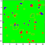
(b)  correlation

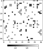
(c)  improved

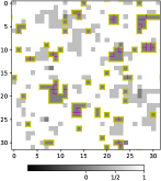
(d)  spin

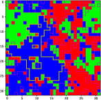
(e)  correlation

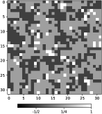
(f)  improved

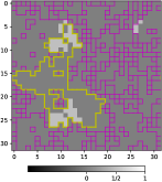
Figure 1: Examples of the spin configuration $\{s_{i}\}$ ((a), (d)), correlation configuration $\{g_{i}(L/2)\}$ ((b), (e)), and improved correlation configuration $\{\tilde{g}_{i}(L/2)\}$ ((c), (f)) of the 2D 3-state Potts model. The upper figures ((a)-(c)) are snapshots at the low temperature, $T=0.9$, and the lower figures ((d)-(f)) are those at the high temperature, $T=1.06$. The borders of FK clusters for spin configuration are drawn by lines. They are copied in improved correlation configuration.

We consider the configuration of the spin correlation with the distance of the half of the system size, $L/2$. We note that this type of correlation function was used along with the generalized scheme for the probability-changing cluster algorithm Tomita and Okabe (2002). For the $q$-state Potts model (including the Ising model), the correlation between two spins becomes 1 for the same spin pair, whereas it becomes $-1/(q-1)$ for the pair of different states. In the improved estimator for the cluster representation, the correlation becomes 1 for the spin pair belonging to the same FK cluster, whereas it becomes 0 for the spins of different clusters. When the embedded algorithm for the continuous spins is used, the projection of spins onto a randomly chosen reflection axis is made. We denote the site-dependent correlation configuration as $g_{i}(L/2)$. For actual calculation, we treat the average value of the $x$-direction and the $y$-direction, that is,

$$g_{i}(L/2)=(g[s_{x_{i},y_{i}},s_{x_{i}+L/2,y_{i}}]+g[s_{x_{i},y_{i}},s_{x_{i},y_{i}+L/2}])/2,$$ (1)

where $g[s,s^{\prime}]$ denotes a spin-spin correlation between a spin pair $s$ and $s^{\prime}$.

In Fig. 1, we show the examples of the spin configuration $\{s_{i}\}$, correlation configuration $\{g_{i}(L/2)\}$, and improved correlation configuration $\{\tilde{g}_{i}(L/2)\}$ of the 2D 3-state Potts model. The spin configuration is generated by the Monte Carlo simulation, and the correlation configuration and the improved correlation configurations are calculated from the spin configuration. The upper figures are snapshots at the low temperature, $T=0.9$, and the lower figures are those at the high temperature, $T=1.06$. Temperatures are measured in the unit of the coupling $J$. We note that the exact second-order transition temperature $T_{c}$ for this model is known as $1/\ln(1+\sqrt{3})\approx 0.995$.

Spins are displayed in one of three colors, red, green, or blue. The ordinary correlation takes a value of $1,-1/2$, or $+1/4$, whereas the improved correlation takes a value of $1,0$, or $+1/2$. The both of correlations from $+1$ to $-1$ are mapped in gray scale from 255 (white) to 0 (black). The permutation of three-state spins yields an essentially identical configuration, and the correlation configurations are invariant under the permutation. The borders of FK clusters for spin configuration are drawn by lines in Figs. 1(a) and (d). They are copied in improved correlation configuration. The border of the largest cluster is drawn by yellow thick line for convenience.

At high temperatures, the spin configurations and the correlation configurations are randomly distributed, and the fluctuation of these quantities gives the susceptibility. In the improved correlation, the cancellation among different FK clusters are automatically satisfied. Figure 1(e) and 1(f) show the difference between the two correlation configurations. While the ordinary correlation configuration in Fig. 1(e) fluctuates in space, a couple of brighter areas in the largest cluster show the improved correlation in Fig. 1(f).

As a supplemental material, we provide animations of the spin configuration, the correlation configuration, and the improved correlation configuration for the 2D Ising model (mp4 files) for convenience Sup . The animations at various temperatures are compared at the low temperature ($T=2.1$), at $T_{c}=2.269$, and at the high temperature ($T=2.4$). The system sizes are $L$=32 and 64.

We use the same technique of supervised learning as Shiina et al. Shiina et al. (2020) for the classification of the phases of spin systems. We consider a fully connected neural network implemented with a standard TensorFlow library Abadi et al. using the 100-hidden unit model to classify the ordered, the BKT, and the disordered phases. For the input layer, we use the improved correlation configurations $\{\tilde{g}_{i}(L/2)\}$. We have used a cross-entropy cost function supplemented with an $L2$ regularization term. The neural networks were trained using the Adam method Kingma and Ba .

(a)

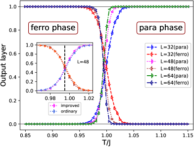
(b)

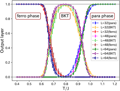
Figure 2: (a) The output layer averaged over a test set as a function of $T$ for the 2D 3-state Potts model. The system sizes are $L$ = 32, 48, and 64. The samples of $T$ within the ranges $0.85\leq T\leq 0.94$ and $1.06\leq T\leq 1.15$ are used for the training data. In the inset, the comparison is made between the results of improved correlation and those of ordinary correlation in the case of $L=48$. The exact $T_{c}$, $1/\ln(1+\sqrt{3})\approx 0.995$, is shown by dashed line for convenience. (b) The same plot for the 2D 6-state clock model. The system sizes are the same. The samples of $T$ within the ranges $0.4\leq T\leq 0.64$, $0.77\leq T\leq 0.83$, and $0.96\leq T\leq 1.2$ are used for the training data.

We first analyzed the 2D 3-state Potts model. The output layer averaged over a test set as a function of $T$ for the 2D 3-state Potts model is shown in Fig. 2(a). The probabilities of predicting the phases, the disordered or the ordered, are plotted for each temperature. The system sizes are $L$ = 32, 48, and 64. The samples of $T$ within the ranges $0.85\leq T\leq 0.94$ and $1.06\leq T\leq 1.15$ were used for the training data. We have not used the samples close to $T_{c}$ for the training data because we assumed the situation that the exact $T_{c}$ is not known. For a whole temperature range, around 35,000 training data sets are used, and we use 500 test data sets for each temperature. Ten independent calculations were performed to provide error analysis. This figure corresponds to Fig. 2(a) of Ref. Shiina et al. (2020), and we again observe that the neural network could successfully classify the disordered and ordered phases using the improved correlation configuration. In the inset of Fig. 2(a), we show the comparison of the results of improved correlation (the present study) and those of the previous study Shiina et al. (2020) of ordinary correlation in the case of $L=48$. We used the same conditions for both training data and test data of improved and ordinary correlations produced from the same spin configurations. The point that the probabilities of predicting two phases are 50% is slightly more close to the exact critical temperature, shown in dashed line in the inset, for the improved correlation, but the difference is small. The advantage of the improved estimator appears at high enough temperatures (compare Fig. 1(f) with 1(e)).

We next consider the 2D 6-state clock model. Because of the discreteness, there are two transitions. One is a higher BKT transition, $T_{2}$, between the disordered and BKT phases, and the other is a lower transition, $T_{1}$, between the BKT and ordered phases. The output layer averaged over a test set as a function of $T$ for the 2D 6-state clock model is shown in Fig. 2(b). The system sizes are $L$ = 32, 48, and 64. The samples of $T$ within the ranges $0.4\leq T\leq 0.64$, $0.77\leq T\leq 0.83$, and $0.96\leq T\leq 1.2$ were used for the low-temperature, mid-range temperature, and high-temperature training data, respectively. The recent numerical estimates of $T_{1}$ and $T_{2}$ for the 6-state clock model are 0.701(5) and 0.898(5), respectively Surungan et al. (2019). This figure corresponds to Fig. 4(a) of Ref. Shiina et al. (2020), and the present figure again shows the successful classification into the three phases.

We have classified the phases of transitions by means of the machine-learning approach by Shiina et al. Shiina et al. (2020) using improved correlation configuration. There is no appreciable difference of accuracy between the use of the correlation configuration and that of the improved correlation configuration. The result indicates that the machine-learning based phase classification is robust; that is, the phase classification does not discriminate the improved correlation configuration from the ordinary one.

Many applications of the loop updating method have been done for quantum systems. Here, we consider the quantum spin 1/2 XY model in two dimensions, which clearly demonstrated the utility of the loop algorithm Harada and Kawashima (1997). The Hamiltonian is written as

$$H=-J\sum_{\langle i,j\rangle}(\hat{S}_{i}^{x}\hat{S}_{j}^{x}+\hat{S}_{i}^{y}\hat{S}_{j}^{y}).$$ (2)

Here, the spin operators $\hat{S}^{x,y}$ are one-half of the Pauli matrices $\sigma^{x,y}$. The summation is taken over the nearest-neighbor pairs. This model exhibits the BKT transition at around $T=0.342$ Harada and Kawashima (1997).

We performed the quantum Monte Carlo simulation using the loop algorithm, and calculated the spatial correlation with the distance of $L/2$. A $D$-dimensional quantum system can be treated as a $(D+1)$-dimensional classical system with an extra dimension of imaginary time. In calculating the spatial correlation, the summation over the imaginary-time axis is taken. The $\hat{S}^{x}$-component of the correlation function is calculated as Brower et al. (1998)

$$\tilde{g}^{x}_{\bm{r}_{i},\bm{r}_{j}} =\frac{4}{\beta^{2}}\int_{0}^{\beta}\int_{0}^{\beta}\hat{S}^{x}(\bm{r}_{i},\tau_{1})\hat{S}^{x}(\bm{r}_{j},\tau_{2})\ d\tau_{1}d\tau_{2}$$

$$=\frac{1}{\beta^{2}}\int_{0}^{\beta}\int_{0}^{\beta}\delta_{\ell}(\bm{r}_{i},\tau_{1};\bm{r}_{j},\tau_{2})\ d\tau_{1}d\tau_{2},$$ (3)

where $\delta_{\ell}(\cdot)$ is the function that returns 1 if the loop of the position $\bm{r}_{i}$ and the time $\tau_{1}$ and that of the position $\bm{r}_{j}$ and the time $\tau_{2}$ belong to the same loop, whereas returns 0 otherwise. Due to the O(2) symmetry of the model, the $\hat{S}^{y}$-component of the correlation function is exactly the same as the $\hat{S}^{x}$-component Brower et al. (1998). The factor 4 is introduced for the comparison of the spin one-half system with the classical model. We checked our calculation by the consistency with the precise calculations at $T=0$ Sandvik and Hamer (1999); Lin et al. (2001).

It is instructive to compare the correlation configurations of the quantum XY model and the classical XY model. In Fig. 3, examples of the snapshots of $\{\tilde{g}_{i}(L/2)\}$ of two models are displayed. At high temperatures above $T_{\mathrm{BKT}}$ ((b), (d)), both improved configurations represent the behavior of finite correlation length. At low temperatures below $T_{\mathrm{BKT}}$ ((a), (c)), they are different from the high-temperature configurations and at the same time they are different from the behavior of the ordered state, which was shown in Fig. 1(c). (Note that the precise estimate of the BKT temperature of the classical XY model is $T_{\mathrm{BKT}}$ = 0.8929 Hasenbusch (2005).)

(a) quantum    $T=0.24$          (b) quantum    $T=0.44$

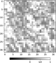
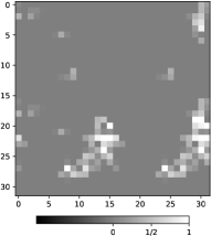
(c) classical    $T=0.6$            (d) classical   $T=1.2$

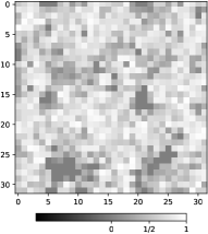
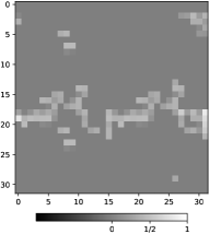
Figure 3: Comparison of snapshots of $\{\tilde{g}_{i}(L/2)\}$ of the 2D quantum ((a), (b)) and classical ((c), (d)) XY models. Examples of snapshots below $T_{\mathrm{BKT}}$ ((a), (c)) and those above $T_{\mathrm{BKT}}$ ((b), (d)) are displayed.

(a)

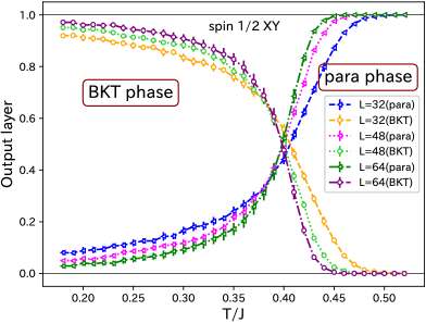
(b)

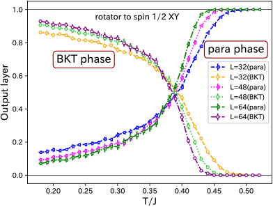
Figure 4: (a) The output layer averaged over a test set as a function of $T$ for the 2D spin 1/2 XY model. The system sizes are $L$ = 32, 48, and 64. The samples of $T$ within the ranges $0.16\leq T\leq 0.32$ and $0.38\leq T\leq 0.54$ are used for the training data. (b) The classification of the quantum XY model using the training data of the classical XY model (plane rotator). The samples of $T$ within the ranges $0.50\leq T\leq 0.84$ and $0.96\leq T\leq 1.30$ for the classical XY model are used for the training data.

The classification of the BKT and paramagnetic phases of the spin 1/2 XY model using the machine-learning technique is shown in Fig. 4(a). The samples of $T$ within the ranges $0.16\leq T\leq 0.32$ and $0.38\leq T\leq 0.54$ were used for the BKT-temperature and high-temperature training data, respectively. If we estimate the value of $T_{\mathrm{BKT}}$ from the point that the probabilities of predicting two phases are 50%, this temperature becomes around $T=0.40$. It is slightly higher than the precise estimate for the infinite system, $T_{\mathrm{BKT}}=0.342$ Harada and Kawashima (1997), although this temperature becomes lower as the system size increases. We also tested the classification of the quantum XY model using the training data of the classical model. For the classical model, not only the classical XY model (plane rotator) but also the anisotropic Heisenberg model with XY interaction was treated. This anisotropic Heisenberg model has out-of-plane fluctuation and the BKT transition temperature is slightly lowered at around $T_{\mathrm{BKT}}=0.70$ Evertz and Landau (1996); Figueiredo et al. (2017). In Fig. 4(b), we show the result of the classification of the quantum XY model using the training data of the classical XY model (plane rotator). We reproduced the BKT transition of the quantum XY model. The same conclusion was obtained when using the anisotropic Heisenberg model as the training data. The classification into two phases is slightly sharper for the anisotropic Heisenberg model than the classical XY model (plane rotator). The opposite direction, using the training data of the quantum model in the classification of the classical models, was also successful.

To summarize, we have proposed a method to use the improved estimator of the correlation configuration in the machine-learning study of the phase classification of spin models. For the classical spin systems, we have demonstrated the machine-learning studies of the 2D 3-state Potts model (the second-order transition) and the 2D 6-state clock model (the BKT transition). The results were compared with those of the previous study Shiina et al. (2020) using the ordinary correlation instead of the improved correlation. The method was also applied to the quantum Monte Carlo simulation using the loop algorithm. We treated the spin 1/2 quantum XY model, and analyzed the BKT transition of the model. We emphasize that the classification scheme based on the training data of the classical XY model can be used for the phase classification of the quantum model. It indicates the universality of the phase transition, and at the same time, the generalized feature of the phase classification based on the machine learning. We also point out the effectiveness of the improved estimators in the loop algorithm to bridge classical and quantum Monte Carlo simulations.

We have opened a door to using the improved estimators for the machine-learning study of quantum systems. It is not trivial whether loop clusters in quantum spin systems can be identified with FK clusters in classical spin systems Nonomura and Tomita (2020). In this study, we clarified that the phase classification using machine learning does not discriminate between loop clusters and FK clusters. The BKT transition of the present study is a thermal phase transition. The investigation of a quantum phase transition at $T=0$ will be interesting. For future studies, we may list up several models for spin and charge degrees of freedom with loop algorithms. Examples are several quantum spin models, strongly-correlated electron models, hard-core boson models, optical lattices, etc.

Another direction of the future study is related to the inverse renormalization group approach Ron et al. (2002). Efthymiou et al. Efthymiou et al. (2019) have proposed a method to increase the size of lattice spin configuration using super-resolution, deep convolutional neural networks. At high temperatures, however, there is a problem that the noise is largely random and difficult to learn. The present improved correlation configuration could reduce this difficulty at high temperatures.

The authors thank Hiroyuki Mori for valuable discussions. This work was supported by a Grant-in-Aid for Scientific Research from the Japan Society for the Promotion of Science Grant Number JP16K05480, JP16K05482. KS is grateful to the A*STAR (Agency for Science, Technology and Research) Research Attachment Programme (ARAP) of Singapore for financial support.

References

- Carleo et al. (2019) G. Carleo, I. Cirac, K. Cranmer, L. Daudet, M. Schuld, N. Tishby, L. Vogt-Maranto, and L. Zdeborová, Rev. Mod. Phys. 91, 045002 (2019).