Spin orientation and magnetostriction of Tb_1-xDy_xFe₂ from first principles

Abstract

The optimal amount of dysprosium in the highly magnetostrictive rare-earth compounds Tb_1-xDy_xFe₂ for room temperature applications has long been known to be $x$=0.73 (Terfenol-D). Here, we derive this value from first principles by calculating the easy magnetization direction and magnetostriction as a function of composition and temperature. We use crystal field coefficients obtained within density-functional theory to construct phenomenological anisotropy and magnetoelastic constants. The temperature dependence of these constants is obtained from disordered local moment calculations of the rare earth magnetic order parameter. Our calculations find the critical Dy concentration required to switch the magnetization direction at room temperature to be $x_{c}$=0.78, with magnetostrictions $\lambda_{111}$=2700 and $\lambda_{100}$=-430 ppm, close to the Terfenol-D values.

I Introduction

The cubic Laves phase compound Terfenol-D (Tb_1-xDy_xFe₂, $x$ = 0.73) has unparalleled magnetostrictive properties at room temperature, developing strains of 1600 ppm when a small magnetic field is applied and rotated between the [100] and [111] crystal directions Abbundi and Clark (1977); Clark (1973); Clark et al. (1977). Originally developed for sonar du Trémolet de Lacheisserie (1993), Terfenol-D has a range of potential applications, including vibrational energy harvesting Staley and Flatau (2005); Deng and Dapino (2017), non-destructive testing Rudd and Myers (2018) and multiferroic devices Wang et al. (2017). The latter concept couples magnetostrictive and piezoelectric materials to control electric polarization (or magnetization) with a magnetic (or electric) field, essential for magnetic sensors or magnetoresistive memory Li et al. (2018).

While remarkable for its magnetostriction, Terfenol-D does suffer from two drawbacks: it is brittle Atulasimha and Flatau (2011) and, due to its reliance on the critical heavy rare earths (REs) Tb and Dy, it is expensive Vincent et al. (2020). Intense research has been aimed at finding new materials with reduced or zero RE content and better mechanical properties, with the notable successes of Fe-Ga and Fe-Al (Galfenol and Alfenol) Clark et al. (2003, 2008). Computational modelling, adopting a first-principles (parameter-free) methodology, provides a complementary approach to experimentally searching for new materials, as well as understanding existing ones Brooks et al. (1991); Richter (1998); Buck and Fähnle (1999); Gavrilenko and Wu (2001); Fähnle and Welsch (2002); Wang et al. (2013). However, despite Terfenol-D’s huge importance as a magnetostrictive material, first-principles modelling has not yet been able to answer a basic question, namely: why is the optimum dysprosium content $x$=0.73?

Experimentally, the question can be answered by considering the spin orientation phase diagram Atzmony et al. (1973), which maps out the preferred (easy) direction of magnetization of Tb_1-xDy_xFe₂ as a function of $x$ and temperature $T$. At $T$=300 K, for $x$ $\leq$ 0.6 the easy direction is along [111]; for $x$ $\geq$ 0.9, it is [100]. The critical concentration $x_{c}$=0.73 lies within the soft boundary between these two regions of the phase diagram, and corresponds to a low magnetocrystalline anisotropy (MCA). The low MCA is essential for the aforementioned applications, since then only a small field is needed to trigger a magnetostrictive response. It is also important to note that this critical concentration $x_{c}$ reduces with temperature Atzmony et al. (1973).

A first-principles understanding of Terfenol-D therefore requires calculating the spin orientation diagram. These have been calculated in the past using crystal field (CF) theory Atzmony et al. (1973); Koon and Williams (1978); Kuz’min (2001); Bowden et al. (2004); Martin et al. (2006), which, although giving physical insight, requires parameters e.g. from experiment or point charge models, which are difficult to fit. For instance, Ref. 22 demonstrates how three different sets of CF parameters can reproduce the same experimental magnetostriction curve for DyFe₂. First-principles calculations are free of these parameters, but are often limited to describing stoichiometric compounds at zero temperature.

Here, we combine non-empirical first-principles calculations with the CF approach in order to calculate the spin orientation diagram of Tb_1-xDy_xFe₂ and the critical concentration $x_{c}(T)$. Our approach takes the recently-introduced yttrium-analogue method of calculating CF coefficients within density-functional theory (DFT) Patrick and Staunton (2019a)— which is numerically stable and avoids problems traditionally associated with describing highly-correlated 4$f$ electrons in DFT— and extends it to compute the phenomenological model parameters associated with magnetostriction. CF theory is then used to calculate the magnetocrystalline and magnetoelastic energies associated with these localized RE-4$f$ electrons. We further include the magnetostrictive contribution from itinerant electrons using the finite temperature DFT-based formulation of the disordered local moment picture. Our calculated spin orientation diagram reproduces experimental measurements of the [111] and [100] easy directions over the full range of temperatures and concentrations. We find the critical concentration $x_{c}$ to be 0.78 at room temperature with magnetostrictions $\lambda_{111}$=2700 and $\lambda_{100}$=-430 ppm, close to the Terfenol-D values.

The rest of our manuscript is organized as follows. Section II describes the theory behind our calculation of the spin orientation diagram. In particular, we introduce the phenomenological expression for the total energy as a function of magnetization direction and strain, and discuss the magnetocrystalline and magnetoelastic constants which enter this expression. We review how the contribution to these constants from RE-4$f$ electrons can be connected to crystal field coefficients, and describe how these coefficients are obtained within DFT. We also discuss the disordered local moment calculations used to obtain the itinerant electron contribution and the temperature dependence of the RE-4$f$ magnetic moments. We then present our results in Sec. III, consisting of the calculated magnetocrystalline and magnetoelastic constants of TbFe₂ and DyFe₂, and then the composition and temperature-dependent spin orientation diagram, which is the main result of this work. Finally in Sec. IV we outline future research directions.

II Methodology

II.1 Spin orientation at zero temperature

Our calculations are based on the following phenomenological expression for the energy of the crystal,

$$E(\bm{\hat{e}},\bm{\varepsilon})=E_{\mathrm{el}}(\bm{\varepsilon})+E_{\mathrm{RE}}(\bm{\hat{e}},\bm{\varepsilon})+E_{\mathrm{itin}}(\bm{\hat{e}},\bm{\varepsilon})$$ (1)

which consists of a magnetization-independent elastic energy $E_{\mathrm{el}}$, a contribution $E_{\mathrm{RE}}$ originating from the 4$f$ electrons localized on the RE atoms, and $E_{\mathrm{itin}}$, which originates from itinerant (delocalized) electrons. $\bm{\varepsilon}$ represents the strain, with components written either in Cartesian form ($\varepsilon_{xx},\varepsilon_{xy}$ etc.) or as linear combinations of these ($\varepsilon^{\alpha}$, $\varepsilon^{\gamma i}$, $\varepsilon^{\epsilon i}$), where $\alpha$, $\gamma$ and $\epsilon$ describe homogeneous, tetragonal and shear strain modes, respectively Clark (1980). $\bm{\hat{e}}$ is a unit vector describing the orientation of the magnetization, which can be alternatively expressed as $\bm{\hat{e}}=(\cos\phi\sin\theta,\sin\phi\sin\theta,\cos\theta)$. The equilibrium strain and magnetization state is taken to be that which minimizes $E(\bm{\hat{e}},\bm{\varepsilon})$.

The magnetization of the entire crystal can be seen as the sum of individual contributions from local magnetic moments, where each local moment with some magnitude $\mu$ is associated with a magnetic atom Györffy et al. (1985). At zero temperature, the local moments form an ordered magnetic structure. Raising the temperature introduces thermal disorder amongst the local moments which generally weakens the overall magnetization, until complete disorder is reached at the Curie temperature Györffy et al. (1985). In the zero temperature case, $\bm{\hat{e}}$ describes equivalently the orientation of a particular local moment or the orientation of the overall magnetization . However, this equivalence does not hold at finite temperature, where the magnetic properties of the crystal are determined as an average over the fluctuating local moments. We concentrate initially on the zero temperature case. The generalization to finite temperature is discussed in Sec. II.6. We now discuss each term in equation 1:

II.1.1 Elastic energy

The elastic energy is quadratic in strain and depends on the three elastic constants $c_{11}$, $c_{12}$ and $c_{44}$ Kittel (1949); Clark (1980):

$$E_{\mathrm{el}}(\bm{\varepsilon}) = \frac{c_{11}}{2}(\varepsilon_{xx}^{2}+\varepsilon_{yy}^{2}+\varepsilon_{zz}^{2})+c_{12}(\varepsilon_{yy}\varepsilon_{zz}+\varepsilon_{zz}\varepsilon_{xx}$$ (2)

$$+\varepsilon_{xx}\varepsilon_{yy})+\frac{c_{44}}{2}(\varepsilon_{xy}^{2}+\varepsilon_{yz}^{2}+\varepsilon_{zx}^{2})$$

Ideally we should calculate these constants from first principles. However, even obtaining zero temperature elastic constants for the stoichiometric end compounds TbFe₂ and DyFe₂ in DFT is not straightforward due to the difficulty in treating the RE-4$f$ electrons Bentouaf et al. (2016). Furthermore, the elastic constants are, in principle, dependent on composition and temperature. For simplicity we instead use a single set of elastic constant values of 141, 65 and 49 GPa for $c_{11}$, $c_{12}$ and $c_{44}$, for all compositions and temperatures. These values were measured experimentally for Tb_0.3Dy_0.7Fe₂ Clark (1980). We have tested the sensitivity of our results to this choice by calculating spin orientation diagrams using different sets of elastic constant values which were either obtained from DFT or measured experimentally, for different compositions Bentouaf et al. (2016); Moulay et al. (2013). The comparison is provided as an Appendix A, and shows the sensitivity to be very weak.

II.1.2 RE-4$f$ electron energy

The energy associated with the RE-4$f$ electrons $E_{\mathrm{RE}}(\bm{\hat{e}},\bm{\varepsilon})$ can be further partitioned as

$$E_{\mathrm{RE}}(\bm{\hat{e}},\bm{\varepsilon})=E_{\mathrm{mca}}(\bm{\hat{e}})+E_{\mathrm{me}}(\bm{\hat{e}},\bm{\varepsilon})$$ (3)

where the MCA energy $E_{\mathrm{mca}}(\bm{\hat{e}})$ depends only on the orientation of the RE-4$f$ magnetic moment, and the magnetoelastic energy $E_{\mathrm{me}}(\bm{\hat{e}},\bm{\varepsilon})$ couples this orientation to the strain. The MCA energy can be written as

$$E_{\mathrm{mca}}(\bm{\hat{e}})=\sum_{l=4,6}\mathcal{K}^{\alpha,l}S^{\alpha,l}(\bm{\hat{e}})$$ (4)

where $\mathcal{K}^{\alpha,l}$ are the anisotropy constants and $S^{X,l}$ are the symmetry basis functions, which are listed in Ref. 26 ($X=\alpha,\gamma,\epsilon$). $\mathcal{K}^{\alpha,l}$ are related to the more conventional anisotropy constants $K_{1}$ and $K_{2}$ as $K_{1}=-2(\mathcal{K}^{\alpha,4}+\frac{1}{22}\mathcal{K}^{\alpha,6})$ and $K_{2}=\mathcal{K}^{\alpha,6}$.

The magnetoelastic energy $E_{\mathrm{me}}(\bm{\hat{e}},\bm{\varepsilon})$ is obtained as the direct product of strain and magnetization basis functions belonging to the same representation Clark (1980):

$$E_{\mathrm{me}}(\bm{\hat{e}},\bm{\varepsilon}) = \varepsilon^{\alpha}\sum_{l=4,6}\mathcal{B}^{\alpha,l}S^{\alpha,l}(\bm{\hat{e}})$$ (5)

$$+\sum_{i=1,2}\varepsilon^{\gamma i}\sum_{l=2,4,6}\mathcal{B}^{\gamma,l}S^{\gamma,l}_{i}(\bm{\hat{e}})$$

$$+\sum_{i=1,2,3}\varepsilon^{\epsilon i}\sum_{l=2,4,6,6^{\prime}}\mathcal{B}^{\epsilon,l}S^{\epsilon,l}_{i}(\bm{\hat{e}})$$

The coefficients $\mathcal{B}^{X,l}$ are the magnetoelastic constants. Note how the lower symmetry of the tetragonal or shear-strained structures ($\gamma$ or $\epsilon$) generates new terms with an $l$=2 dependence on magnetization direction.

Evaluating $E_{\mathrm{RE}}(\bm{\hat{e}},\bm{\varepsilon})$ therefore requires knowing the anisotropy and magnetoelastic constants $\mathcal{K}^{\alpha,l}$ and $\mathcal{B}^{X,l}$. We discuss the calculation of these constants within the framework of the single-ion model and crystal field theory in Secs. II.2, II.3 and II.4.

II.1.3 Itinerant electron energy

The remaining term $E_{\mathrm{itin}}(\bm{\hat{e}},\bm{\varepsilon})$ accounts for the MCA and magnetoelastic contributions to the energy not already included in the RE-4$f$ term, i.e. those coming from itinerant electrons. These itinerant electrons are mainly Fe-3$d$ in character, with a lesser contribution from the RE-5$d$ electrons Brooks et al. (1991). The relative importance of $E_{\mathrm{RE}}$ and $E_{\mathrm{itin}}$ to the magnetostriction can be assessed by comparing TbFe₂ or DyFe₂ to their isostructural counterpart GdFe₂. These three compounds have the same itinerant electronic structure, and therefore should have comparable $E_{\mathrm{itin}}$. However, $E_{\mathrm{RE}}$ is zero in GdFe₂ due to the filled Gd-4$f$ spin subshell having zero orbital moment Kuz’min and Tishin (2008). Comparing the experimentally-measured magnetostrictions of the different compounds, we find TbFe₂ has a magnetostriction which is 50 times larger than GdFe₂ Clark (1980), showing that $E_{\mathrm{RE}}$ is the dominant contribution to equation 1. Nevertheless, for completeness we still include $E_{\mathrm{itin}}$ in our analysis.

In principle, $E_{\mathrm{itin}}(\bm{\hat{e}},\bm{\varepsilon})$ can be split into MCA and magnetoelastic contributions as in equation 3, with a different set of constants. In practice (Sec. III.1), we find the MCA contribution to be negligible, and also that it is sufficient only to consider the $l=2$ term in the magnetoelastic expansion. We therefore have

$$E_{\mathrm{itin}}(\bm{\hat{e}},\bm{\varepsilon})=\mathcal{B}^{\gamma,2}_{\mathrm{itin}}\sum_{i=1,2}\varepsilon^{\gamma i}S^{\gamma,2}_{i}(\bm{\hat{e}})+\mathcal{B}^{\epsilon,2}_{\mathrm{itin}}\sum_{i=1,2,3}\varepsilon^{\epsilon i}S^{\epsilon,2}_{i}(\bm{\hat{e}})$$ (6)

Due to their itinerant electron origin, the constants $\mathcal{B}^{\gamma,2}_{\mathrm{itin}}$ and $\mathcal{B}^{\epsilon,2}_{\mathrm{itin}}$ cannot be obtained from crystal field theory. They are however amenable to treatment in the DFT-based disordered local moment picture Györffy et al. (1985); Marchant et al. (2019). We describe these calculations in Sec. II.5.

II.2 Single-ion treatment of RE-4$f$ contribution and modelling of alloys

We calculate the RE-4$f$ energy $E_{\mathrm{RE}}(\bm{\hat{e}},\bm{\varepsilon})$ within the single-ion model Callen and Callen (1966), which has been used to great effect to understand the behavior of RE-transition metal compounds for many years Kuz’min and Tishin (2008). In this model, the magnetic moment associated with the 4$f$ electrons localized on a particular RE ion behaves independently of its neighbours, which is a reasonable approximation Kuz’min (2001) given the highly-localized nature of these electrons and the relatively weak RE-RE magnetic interactions measured in neutron scattering experiments Loewenhaupt et al. (1996). The 4$f$ electrons localized at different RE sites experience the same potential, which is an atomic-like central potential plus a contribution from the surrounding crystal field. The RE-4$f$ electrons also all experience an exchange field originating from the itinerant electrons and possibly an external magnetic field, which both drive magnetic order Kuz’min and Tishin (2008).

The crystal field is supposed to derive from the valence electronic structure, and therefore is insensitive to (a) the orientations of surrounding RE-4$f$ localized moments, and (b) the chemical species (Tb or Dy) of surrounding RE ions (since these species have the same $6s^{2}5d$ valence electronic structure). This latter aspect allows a simple treatment of Tb-Dy alloying within the single-ion model, since each RE ion is independent: for a given composition Tb_1-xDy_xFe₂, the RE-4$f$ energy per ion is a superposition of the Tb and Dy contributions,

$$E_{\mathrm{RE}}(\bm{\hat{e}},\bm{\varepsilon})=(1-x)E_{\mathrm{Tb}}(\bm{\hat{e}},\bm{\varepsilon})+xE_{\mathrm{Dy}}(\bm{\hat{e}},\bm{\varepsilon}),$$ (7)

where now $E_{\mathrm{Tb}}$ and $E_{\mathrm{Dy}}$ can be seen as the RE-4$f$ energy contributions calculated for the end compounds TbFe₂ and DyFe₂, respectively. These end compounds each have their own set of two anisotropy and nine magnetoelastic constants, so to evaluate $E_{\mathrm{RE}}$ for an arbitrary $x$ we require 22 constants in total.

II.3 RE anisotropy and magnetoelastic constants from crystal field theory

In the single-ion central potential, the RE-4$f$ electrons form atomic-like eigenstates $|L,S,J,M_{J}\rangle$, where $L$ and $S$ are determined by Hund’s rules, $J=L+S$ for Tb and Dy, and $M_{J}=J,J-1,...,-J$ Griffith (1961). Now, we should construct a Hamiltonian for the RE-4$f$ electrons including the crystal, exchange and external fields, and diagonalize it within the manifold of states with different $M_{J}$ Patrick and Staunton (2019b). Without the crystal and external fields, the ground state will be $|L,S,J,-J\rangle$, with the quantization axis (magnetic moment direction) aligned with the exchange field. Taking this axis as $\bm{\hat{z}}$, the RE-4$f$ electron density $\rho^{(\bm{\hat{z}})}_{4f}(\bm{r})$ associated with $|L,S,J,-J\rangle$ is given by Sievers (1982):

$$\rho^{(\bm{\hat{z}})}_{4f}(\bm{r})=n^{0}_{4f}(r)\sum_{l=2,4,6}\mathcal{A}_{l}\left(\frac{2l+1}{4\pi}\right)^{\frac{1}{2}}Y_{l0}(\bm{\hat{r}})$$ (8)

Here, $n^{0}_{4f}(r)$ is the radial density calculated for the unperturbed central potential Kuz’min and Tishin (2008), and $Y_{lm}(\bm{\hat{r}})$ are complex spherical harmonics. $\mathcal{A}_{l}$ are RE-dependent numerical factors formed from $J$ and Stevens coefficients, which for Tb³⁺ are $\mathcal{A}_{2}$ = -(1/3), $\mathcal{A}_{4}$ = (1/11) and $\mathcal{A}_{6}$ = -(5/429), and for Dy³⁺ are $\mathcal{A}_{2}$ = -(1/3), $\mathcal{A}_{4}$ = -(4/33), and $\mathcal{A}_{6}$ = (25/429) Sievers (1982); Stevens (1952). The RE-4$f$ charge density $\rho^{(\bm{\hat{e}})}_{4f}(\bm{r})$ corresponding to a general magnetic moment direction $\bm{\hat{e}}$ is obtained from equation 8 by making the substitution $Y_{l0}(\bm{\hat{r}})\rightarrow\sum_{m}e^{-im\phi}d^{(l)}_{m0}(\theta)Y_{lm}(\bm{\hat{r}})$, where the functions $d^{(l)}_{m0}(\theta)$ are equal to $[(l-m)!/(l+m)!]^{\frac{1}{2}}P^{m}_{l}(\cos\theta)$ and $P^{m}_{l}(x)$ are the associated Legendre polynomials Edmonds (1960).

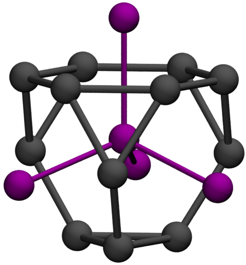
Figure 1: The local $T_{d}$ environment of the RE atom in the cubic Laves phase, showing nearest neighbor (Fe, grey) and next-nearest neighbor (RE, purple) atoms. The RE-RE bonds are oriented along the $\langle 111\rangle$ directions.

The crystal field (CF) characterizes the nonspherical components of the potential at the RE site, $V(\bm{r})=\sum_{lm}V_{lm}(r)Y_{lm}(\bm{\hat{r}})$. If the exchange field is sufficiently strong compared to the CF, the latter will not mix states of different $M_{J}$. Then, the energy shift due to the CF is obtained from first order perturbation theory as

$$E_{4f}(\bm{\hat{e}})=\sum_{l=2,4,6}\mathcal{A}_{l}\sum_{m}(-1)^{m}B_{l-m}e^{-im\phi}d^{(l)}_{m0}(\theta)$$ (9)

where the CF coefficients Patrick and Staunton (2019a) have been introduced as:

$$B_{lm}=\left(\frac{2l+1}{4\pi}\right)^{\frac{1}{2}}\int r^{2}n^{0}_{4f}(r)V_{lm}(r)dr.$$ (10)

For REFe₂ in the cubic Laves phase (Fig. 1), the RE atoms sit at sites with $T_{d}$ symmetry, so the only nonzero CF coefficients which appear in equation 9 are $B_{40}$, $B_{4\pm 4}$, $B_{60}$ and $B_{6\pm 4}$; only $B_{40}$ and $B_{60}$ are independent Bradley and Cracknell (1972).

Here we will assume that the exchange field is strong enough that $E_{4f}(\bm{\hat{e}})$ is given by equation 9, and also that the exchange field and magnetization are isotropic. Then, $E_{4f}$ is the only contribution to the energy which depends on the magnetization angle. At zero strain we can equate $E_{4f}$ and $E_{\mathrm{mca}}$ (equations 4 and 9) to obtain

$$\mathcal{K}^{\alpha,4}=\frac{5}{2}\mathcal{A}_{4}B_{40};\ \mathcal{K}^{\alpha,6}=\frac{231}{2}\mathcal{A}_{6}B_{60}.$$ (11)

Next, to obtain the magnetoelastic constants $\mathcal{B}^{X,l}$ we consider the modifications to the CF coefficients when three different strain modes are applied: $\varepsilon_{xx}=\varepsilon_{yy}=\varepsilon_{zz}=\varepsilon_{I}$ (isotropic), $\varepsilon_{zz}=-2\varepsilon_{xx}=-2\varepsilon_{yy}=\varepsilon_{T}$ (tetragonal) and $\varepsilon_{xy}=\varepsilon_{yz}=\varepsilon_{zx}=\varepsilon_{S}$ (shear). For the shear deformation it is convenient to work in a rotated co-ordinate system where the $z$ axis coincides with the [111] direction. Then, aside from altering the CF coefficients which are already nonzero in the unstrained $T_{d}$ environment, the tetragonal and shear strains affect $E_{4f}(\bm{\hat{e}})$ in equation 9 by generating a nonzero $B_{20}$ coefficient.

Denoting the strain-induced shifts in CF coefficients as $\Delta B_{lm}$, our calculations (Sec. III.1) find that these shifts can be described well by the linear relation $\Delta B_{lm}=\frac{dB_{lm}}{d\varepsilon_{X}}\varepsilon_{X}$. Inserting these relations into equation 9 and comparing to equation 5 gives each magnetoelastic constant in terms of the strain derivative of a CF coefficient, for instance,

$$\mathcal{B}^{\gamma,2}=\frac{2}{3}\mathcal{A}_{2}\frac{dB_{20}}{d\varepsilon_{T}};\ \mathcal{B}^{\epsilon,2}=\mathcal{A}_{2}\frac{dB_{20}}{d\varepsilon_{S}}.$$ (12)

II.4 DFT calculation of CF coefficients

Equations 11 and 12 show how the anisotropy and magnetoelastic constants can be obtained from the CF coefficients $B_{lm}$ and their strain derivatives $dB_{lm}/d\varepsilon_{X}$. These are the quantities which we calculate from first principles within the yttrium-analogue method Patrick and Staunton (2019a). In this approach, the potential $V(\bm{r})$ which determines the CF coefficients is calculated within DFT for the “Y-analogue” of TbFe₂ or DyFe₂, which is YFe₂. Specifically, the components $V_{lm}(r)$ in equation 10 are found from the angular decomposition of the self-consistent Kohn-Sham potential calculated for the desired REFe₂ structure, where the RE is replaced with Y.

We have previously used the Y-analogue method to calculate CF coefficients for various RE/transition-metal compounds Patrick and Staunton (2019a), demonstrating its applicability to describe temperature and pressure-induced spin-reorientation transitions in the RECo₅ compounds Patrick and Staunton (2019b); Kumar et al. (2020a, b). Substituting Tb or Dy with Y to calculate the crystal field is consistent with the assumptions of the single-ion model Callen and Callen (1966), namely that the CF depends on the valence electronic structure and not on the RE-4$f$ electrons themselves. Since the RE ions are in the 3$+$ state and therefore are isovalent (two $s$ and a single $d$ electron), we expect the CF of YFe₂ to be a good approximation for TbFe₂ or DyFe₂. Indeed, using the Y-analogue ensures that there is no double-counting of the RE-4$f$ electrons in equation 10. Any DFT implementation can be used to calculate the CF coefficients, providing the valence charge density is described accurately.

Equation 10 also contains the RE-4$f$ electron density calculated for the unperturbed central potential $n^{0}_{4f}(r)$. Previously we calculated $n^{0}_{4f}(r)$ within self-interaction-corrected DFT Lüders et al. (2005); Däne et al. (2009) for a number of compounds and found that, for a given RE element, it was highly insensitive to the crystalline environment Patrick and Staunton (2019a). Therefore when calculating CF coefficients we use the same previously calculated RE-dependent functions ($n^{0}_{4f,\mathrm{Tb}}(r)$ or $n^{0}_{4f,\mathrm{Dy}}(r)$  ) for all strain states.

II.5 Itinerant electron contribution

The itinerant electrons are (by definition) delocalized, and are responsible for generating the crystal field rather than simply being influenced by it. Accordingly, the CF picture is not appropriate to describe their contribution to the magnetostriction. However, itinerant electron magnetism is amenable to a fully first-principles treatment within DFT Györffy et al. (1985). In Sec. II.1.3 we used GdFe₂ as a comparison system to understand the importance of $E_{\mathrm{itin}}(\bm{\hat{e}},\bm{\varepsilon})$ to the magnetostriction, since it has the same valence electronic structure but zero CF contribution from the filled Gd-4$f$ spin subshell. Building on this idea, we take $E_{\mathrm{itin}}(\bm{\hat{e}},\bm{\varepsilon})$ to be the same for Tb_1-xDy_xFe₂ and GdFe₂, and calculate the latter directly. Similarly to using the Y-analogue, this approach avoids any double-counting of the CF contribution. However, using Gd rather than Y to calculate $E_{\mathrm{itin}}$ has the advantage of capturing any additional on-site polarization of the valence electrons by the large spin moments possessed by Gd, Tb and Dy Patrick et al. (2018); Patrick and Staunton (2018).

We calculate $E_{\mathrm{itin}}(\bm{\hat{e}},\bm{\varepsilon})$ for GdFe₂ using the same method demonstrated recently for bcc Fe and Fe-Ga alloys Marchant et al. (2019). This approach is a Green’s function, multiple-scattering theory-based formulation of the disordered local moment picture within DFT (DFT-DLM Györffy et al. (1985)) which as discussed in Sec. II.6 allows the treatment of finite temperature magnetic disorder. The filled Gd-4$f$ spin subshell is treated efficiently using the local self-interaction correction (LSIC) Lüders et al. (2005). Quantities related to the magnetic anisotropy are obtained by solving the relativistic single-site scattering problem and applying the torque method Staunton et al. (2006). As described in Ref. Marchant et al. (2019), calculating the derivative of the total energy with respect to magnetization angle for different strain states allows the anisotropy and magnetoelastic constants to be obtained.

II.6 Generalization to finite temperature

The methodology described above is sufficient to evaluate equation 1 assuming that all the individual magnetic moments are ordered, corresponding to zero temperature. At finite temperature $T$, equation 1 takes a slightly different form:

$$E(\bm{\hat{n}},\bm{\varepsilon},T)=E_{\mathrm{el}}(\bm{\varepsilon})+E_{\mathrm{RE}}(\bm{\hat{n}},\bm{\varepsilon},T)+E_{\mathrm{itin}}(\bm{\hat{n}},\bm{\varepsilon},T)$$ (13)

The new quantity introduced is the unit vector $\bm{\hat{n}}$ which describes the orientation of the magnetization of the entire crystal, and therefore represents an average over the individual magnetic moments. The degree of magnetic order is quantified through the temperature-dependent order parameters $m_{\mathrm{Tb}}$, $m_{\mathrm{Dy}}$ and $m_{\mathrm{itin}}$ which take values between 1 (zero temperature, fully ordered) and 0 (above the Curie temperature, fully disordered). The relationship between the orientation of the individual moments and their average is given by, for instance, $\langle\bm{\hat{e}_{\mathrm{Tb}}}\rangle_{T}=m_{\mathrm{Tb}}(T)\bm{\hat{n}}$ where $\langle\rangle_{T}$ denotes the statistical mechanical thermal average taken (in this example) over the individual moments of all Tb ions. More generally, the finite and zero temperature energies in equations 1 and 13 are related simply as $E(\bm{\hat{n}},\bm{\varepsilon},T)=\langle E(\bm{\hat{e}},\bm{\varepsilon})\rangle_{T}$.

Evaluating the thermal average $\langle\rangle_{T}$ requires a model for the statistical mechanics of the magnetic moments. The DFT-DLM framework employs a Heisenberg-like Hamiltonian for this purpose Györffy et al. (1985). The probability that a moment is aligned along a direction $\bm{\hat{e}}$ at $T$ is given by $P_{\bm{\hat{n}}}(\bm{\hat{e}})\propto\exp[\beta h\bm{\hat{n}}\cdot\bm{\hat{e}}]$, where $1/\beta=k_{B}T$. The Weiss field felt by each local moment $h(T)$ is determined self-consistently from DFT-DLM calculations at a given temperature using the iterative scheme described in Ref. Patrick et al. (2017). The self-consistency condition ensures (a) that the free energy is minimized, and (b) that the model approximates the true statistical mechanics of the moments as closely as possible Györffy et al. (1985). Each crystallographically inequivalent magnetic atom (Tb, Dy and Fe) experiences its own Weiss field, and within the model the order parameter and Weiss fields are linked according to (again taking Tb as an example):

$$m_{\mathrm{Tb}}(T)=\coth(\beta h_{\mathrm{Tb}}(T))-\frac{1}{\beta h_{\mathrm{Tb}}(T)}$$ (14)

II.6.1 Thermally-averaged rare earth contribution

Recalling that in the crystal field picture the CF is independent of the RE moment orientations, and that the anisotropy and magnetoelastic constants are determined by the CF coefficients, the thermal average of the RE contribution is determined by solely by the average of the symmetry basis functions, e.g.

$$E_{\mathrm{mca}}(\bm{\hat{n}},T)=\sum_{l=4,6}\mathcal{K}^{\alpha,l}\langle S^{\alpha,l}(\bm{\hat{e}})\rangle_{T}.$$ (15)

Due to the local nature of the probability function $P_{\bm{\hat{n}}}(\bm{\hat{e}})$, the general arguments of Callen and Callen Callen and Callen (1966) can be used to show

$$\langle S^{X,l}(\bm{\hat{e}})\rangle_{T}=f_{l}(m)S^{X,l}(\bm{\hat{n}})$$ (16)

where the functions $f_{l}(m)$ depend on $m$ as $m^{\frac{l(l+1)}{2}}$ and $m^{l}$ at low and high temperature respectively Callen and Callen (1966). Then, the explicit expression for the RE contribution at finite temperature is

$$E_{\mathrm{RE}}(\bm{\hat{n}},\bm{\varepsilon},T) = \sum_{l=4,6}\mathcal{K}^{\alpha,l}_{\mathrm{RE}}(T)S^{\alpha,l}(\bm{\hat{n}})$$

$$+\varepsilon^{\alpha}\sum_{l=4,6}\mathcal{B}^{\alpha,l}_{\mathrm{RE}}(T)S^{\alpha,l}(\bm{\hat{n}})$$

$$+\sum_{i=1,2}\varepsilon^{\gamma i}\sum_{l=2,4,6}\mathcal{B}^{\gamma,l}_{\mathrm{RE}}(T)S^{\gamma,l}_{i}(\bm{\hat{n}})$$

$$+\sum_{i=1,2,3}\varepsilon^{\epsilon i}\sum_{l=2,4,6,6^{\prime}}\mathcal{B}^{\epsilon,l}_{\mathrm{RE}}(T)S^{\epsilon,l}_{i}(\bm{\hat{n}})$$

where the finite and zero-temperature constants are simply related by $f_{l}$,

$$\mathcal{K}^{\alpha,l}_{\mathrm{RE}}(T)=\mathcal{K}^{\alpha,l}_{\mathrm{RE}}f_{l}(m_{\mathrm{RE}}(T))$$

$$\mathcal{B}^{X,l}_{\mathrm{RE}}(T)=\mathcal{B}^{X,l}_{\mathrm{RE}}f_{l}(m_{\mathrm{RE}}(T))$$ (18)

and the RE subscript has been inserted as a reminder that the constants and order parameters are calculated either for TbFe₂ or DyFe₂. The RE contribution for the Tb_1-xDy_xFe₂ alloy is obtained through the same linear mixing as at zero temperature, as in equation 7.

The temperature dependence of $E_{\mathrm{RE}}(\bm{\hat{n}},\bm{\varepsilon},T)$ is therefore fixed by the order parameter dependences $m_{\mathrm{Tb}}(T)$ and $m_{\mathrm{Dy}}(T)$, which we determine through finite-temperature, LSIC DFT-DLM calculations on TbFe₂ and DyFe₂. The calculations were performed according to the methodology described in detail in Ref. Patrick and Staunton (2018), and the reader is referred there for a more complete discussion of the underlying theory and technical details of the DFT-DLM scheme.

II.6.2 Thermally-averaged itinerant electron contribution

Performing the thermal average on $E_{\mathrm{itin}}$ gives, in analogy with equation LABEL:eq.ERET,

$$E_{\mathrm{itin}}(\bm{\hat{n}},\bm{\varepsilon},T) = \mathcal{B}^{\gamma,2}_{\mathrm{itin}}(T)\sum_{i=1,2}\varepsilon^{\gamma i}S^{\gamma,2}_{i}(\bm{\hat{n}})$$ (19)

$$+\mathcal{B}^{\epsilon,2}_{\mathrm{itin}}(T)\sum_{i=1,2,3}\varepsilon^{\epsilon i}S^{\epsilon,2}_{i}(\bm{\hat{n}})$$

The finite temperature magnetoelastic constants are obtained from DFT-DLM calculations on GdFe₂, which give directly the temperature dependence of $\mathcal{B}^{X,2}_{\mathrm{itin}}$. As found previously for bcc Fe Marchant et al. (2019), the $\mathcal{B}^{X,2}_{\mathrm{itin}}$ constants do not follow an $f_{2}(m_{\mathrm{itin}})$ dependence on the order parameter. This observation reflects the itinerant origin of the magnetic anisotropy, compared to the single-ion description of the RE moments Staunton et al. (2006).

II.6.3 The need for a phenomenological model

It is reasonable to ask, given that LSIC DFT-DLM calculations can be used to obtain the itinerant electron magnetostriction and also the temperature dependence of the RE order parameters in TbFe₂ and DyFe₂, why we should not perform the entire calculation in the DFT-DLM framework without any reference to crystal field theory. The technical difficulty is that the DFT-DLM calculations are performed within the atomic sphere approximation (ASA) Györffy and Stocks (1979), which means that nonspherical components of the potential at the RE site (i.e. the crystal field) are poorly described in the DFT-DLM calculation of the RE anisotropy. As a result, a separate treatment of the CF is required. In turn, it is important that the calculated energy contribution associated with the itinerant electron anisotropy is free of any contribution from the localized RE-4$f$ electrons interacting with the CF, otherwise this contribution would be counted both in $E_{\mathrm{itin}}$ and $E_{\mathrm{RE}}$ in equation 1. Calculating the itinerant contribution for GdFe₂, which has no CF anisotropy, ensures that this is the case. Similarly, the assumptions of the CF model mean that the CF coefficients themselves should not depend on the asphericity of the RE-4$f$ electrons. This requirement is satisfied by using the Y-analogue model, where the RE-4$f$ electrons do not enter the calculation of the CF potential at all Patrick and Staunton (2019a). These same considerations led us to adopt a similar scheme in the calculation of finite temperature anisotropy of the RCo₅ compounds Patrick and Staunton (2019b).

II.7 Computational details

Crystal field coefficients were calculated for YFe₂ within the projector-augmented formulation of DFT as implemented in the GPAW code Enkovaara et al. (2010), using the local spin-density approximation (LSDA) for exchange and correlation Vosko et al. (1980). A plane wave basis set with a 1200 eV energy cutoff and a 20$\times$20$\times$20 $k$-point sampling was used, as in Ref. 25. A lattice constant of 7.341 Å was used throughout for the equilibrium (cubic) structure, which is the experimentally-measured value for TbFe₂ at room temperature Andreev (1995); the value for DyFe₂ is very similar (7.338 Å). The dependence of the order parameters on temperature were calculated within DFT-DLM Györffy et al. (1985) with the LSIC applied Patrick and Staunton (2018), using the ASA with Wigner-Seitz radii of 1.90 Å for the RE atoms, with angular momentum expansions truncated at $l_{\mathrm{max}}=3$. The same computational setup was used to calculate the temperature-dependent magnetoelastic constants associated with the itinerant electrons for GdFe₂, using the torque method as described in Refs. 33 and 49.

III Results

III.1 Anisotropy and magnetoelastic constants

	$\mathcal{K}^{\alpha,4}$	$\mathcal{K}^{\alpha,6}$	$\mathcal{B}^{\alpha,4}$	$\mathcal{B}^{\alpha,6}$	$\mathcal{B}^{\gamma,2}$	$\mathcal{B}^{\gamma,4}$	$\mathcal{B}^{\gamma,6}$	$\mathcal{B}^{\epsilon,2}$	$\mathcal{B}^{\epsilon,4}$	$\mathcal{B}^{\epsilon,6}$	$\mathcal{B}^{\epsilon,6^{\prime}}$	$\mathcal{B}^{\gamma,2}_{\mathrm{itin}}$	$\mathcal{B}^{\epsilon,2}_{\mathrm{itin}}$
TbFe2	14.10	11.20	-22.87	-27.88	74.69	28.08	6.96	-844.24	258.17	7.22	-4.20	-7.25	33.24
DyFe2	-17.34	-47.52	28.14	116.89	77.12	-30.87	-29.43	-794.88	-307.96	-33.07	17.79	-7.25	33.24

Table 1: Anisotropy and magnetoelastic constants in MJm^-3 calculated for TbFe₂ and DyFe₂.

We previously reported Y-analogue calculations of the CF coefficients of TbFe₂ and DyFe₂ Patrick and Staunton (2019a). The values of $\mathcal{K}^{\alpha,4}$ and $\mathcal{K}^{\alpha,6}$ calculated from equation 11 are given in Table 1. Importantly, due to the differences in $\mathcal{A}_{4}$ and $\mathcal{A}_{6}$ for Tb³⁺ and Dy³⁺, $\mathcal{K}^{\alpha,l}$ have opposite signs for TbFe₂ and DyFe₂ so favor different magnetization directions. From the linear mixing of equation 7, we note that a Dy content of $x=0.45$ would lead to a zero value of $\mathcal{K}^{\alpha,4}$.

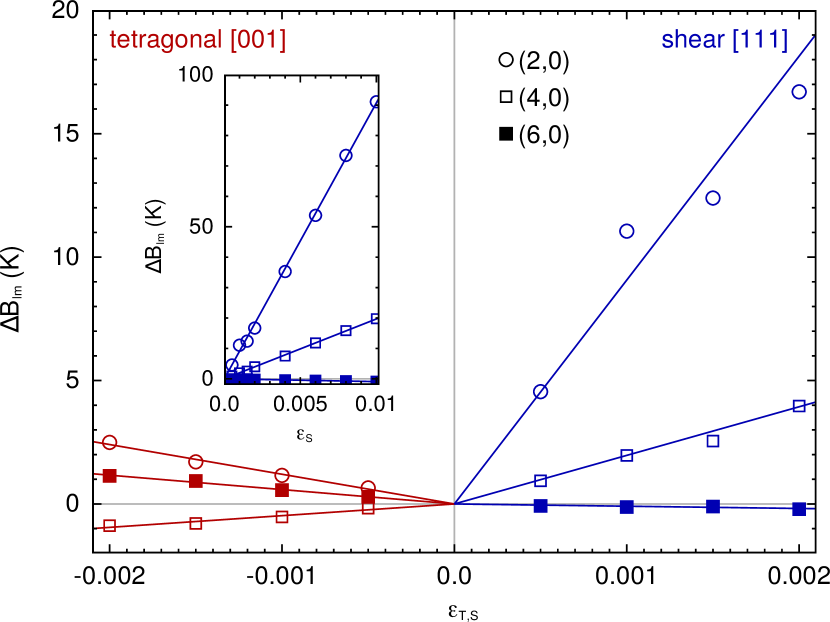
Figure 2: Change in crystal field coefficients $\Delta B_{lm}$ for TbFe₂ for different $(l,m)$ with a shear strain $\varepsilon_{S}$ (blue) or a tetragonal strain $\varepsilon_{T}$ (red) applied. The inset shows $\Delta B_{lm}$ for a larger variation in $\varepsilon_{S}$. The straight lines are fits to the calculations.

Now considering the magnetoelastic constants associated with the RE, in Fig. 2 we plot the strain-induced change in the CF coefficients $\Delta B_{lm}$ for TbFe₂, for $(l,m)$ = (2,0), (4,0) and (6,0). We show $\Delta B_{lm}$ for both tetragonal ($\varepsilon_{T}$) and shear ($\varepsilon_{S}$) strains. Following convention, we divide the CF coefficients by $k_{B}$ so that the quantities have dimensions of temperature.

Although there is some numerical noise in $\Delta B_{20}$ evident for small shear strains $\varepsilon_{S}$, $\Delta B_{lm}$ is linear in $\varepsilon$ over the range of strains considered. Indeed, extending the calculations to larger shear strains confirms this linear relation out to at least $\varepsilon_{S}=0.01$ (inset of Fig. 2). Then, the most striking feature of Fig. 2 is the strong dependence of $B_{20}$ on $\varepsilon_{S}$. At $\varepsilon_{S}$ = 0.002, $\Delta B_{20}$ is 17 K, compared to 2 K for $\varepsilon_{T}$ at -0.002. The corresponding difference between shear and tetragonal strains is much reduced at larger $(l,m)$ values, with $\Delta B_{40}$ = 4 K and -1 K and $\Delta B_{60}$ = 0 K and 1 K respectively.

Converting these derivatives into magnetoelastic constants through relations like equation 12 gives the values shown in Table 1. The large value of $\frac{dB_{20}}{d\varepsilon_{S}}$ is reflected in the coefficient $\mathcal{B}^{\epsilon,2}$, which is an order of magnitude larger than $\mathcal{B}^{\gamma,2}$. Since $\mathcal{B}^{\epsilon,2}$ is negative, this term will favor positive strains along [111]. Furthermore, $\mathcal{B}^{\epsilon,2}$ is the same sign for both TbFe₂ and DyFe₂, since $\mathcal{A}_{2}$ is identical for Tb³⁺ and Dy³⁺ Sievers (1982); Stevens (1952). Therefore, unlike $\mathcal{K}^{\alpha,4}$, there is no cancellation of $\mathcal{B}^{\epsilon,2}$ in the alloy. It is this aspect which allows Tb_1-xDy_xFe₂ to have simultaneously a large magnetostriction and small anisotropy.

Now considering the itinerant electrons, our DFT-DLM calculations on GdFe₂ find the contribution to the MCA to be negligible (of order 1 Jm^-3). The magnetoelastic constants are more significant, and their zero temperature values are given in Table 1 (we stress again that their temperature dependence is more complicated than $f_{l}(m)$) Marchant et al. (2019). The magnetoelastic contribution is well described by constants with $l=2$ only. $\mathcal{B}^{\gamma,2}_{\mathrm{Fe}}$ and $\mathcal{B}^{\epsilon,2}_{\mathrm{Fe}}$ are calculated to have the same sign as observed experimentally for bcc Fe Wedler et al. (2000), but their magnitudes are enhanced (-7.1 and 33 MJm^-3). However, the itinerant electrons still contribute much less than the RE at all of the temperatures considered here.

III.2 Easy directions and magnetostrictions at zero temperature

Using the constants reported in Table 1 we can construct the phenomenological energy for an arbitrary strain, magnetization and composition. Considering the zero temperature case first (equation 1), minimizing $E(\bm{\hat{e}},\bm{\varepsilon})$ with respect to magnetization direction and strain for the end compounds TbFe₂ and DyFe₂ finds easy directions of [111] and [100] respectively. The calculated fractional changes in length along [111] and [100] for TbFe₂ and DyFe₂ are $\lambda_{111}^{\mathrm{TbFe_{2}}}$ = 5200 ppm and $\lambda_{100}^{\mathrm{DyFe_{2}}}$ = -780 ppm at 0 K. Comparing to experimentally-measured values of 4400 and -70 ppm Clark et al. (1977) shows correct qualitative behaviour and numerical agreement within $\sim$1000 ppm, or 0.1% strain; in relative terms, the agreement for $\lambda_{100}^{\mathrm{DyFe_{2}}}$ is less good than for TbFe₂.

Now considering the alloy through equation 7 we find a [111] easy direction for all values of $x$ below $x_{c}=0.56$, above which the easy direction switches abruptly to [100]. This is some way off the experimental optimal concentration of $x=0.73$, but we have not yet included temperature effects. It is also interesting to recompute the magnetization direction ignoring the magnetoelastic contribution to the energy. Then, $x_{c}$ is found to be 0.45, the same value which cancelled $\mathcal{K}^{\alpha,4}$.

III.3 Spin orientation diagram

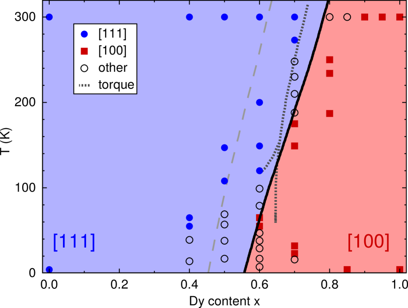
Figure 3: The easy direction of magnetization of Tb_1-xDy_xFe₂, calculated by minimizing $E(\bm{\hat{n}},\bm{\varepsilon},x,T)$ (red and blue shaded regions). The symbols are experimental measurements of the easy direction using Mössbauer spectroscopy Atzmony et al. (1973, 1977). The dotted lines mark the boundaries between different magnetization directions extracted from torque magnetometry Williams et al. (1980), where above 150 K the boundary is between [111] and [100], and below encloses a region of intermediate magnetization direction. The dashed line is the [111]/[100] boundary obtained by minimizing $E_{\mathrm{MCA}}$ only.

We now consider finite temperature, and minimize $E(\bm{\hat{n}},\bm{\varepsilon},T)$ (equation 13) for a grid of $(x,T)$ values. The resulting spin orientation diagram is shown in Fig. 3. As at zero temperature, the easy directions are found either to be [111] or [100] (blue or red regions), and increased Dy content favours [100] magnetization. However, at higher temperatures more Dy is required to maintain the [100] magnetization, i.e. $x_{c}$ increases with temperature.

The reason for the increase in $x_{c}$ is due to the behavior of the RE order parameters with temperature. Our DFT-DLM calculations find that the Dy order parameter $m_{\mathrm{Dy}}$ decreases more quickly with $T$ than $m_{\mathrm{Tb}}$, something which can also be inferred from experimental magnetization measurements Clark (1980). This behavior can be understood as the lower spin moment of Dy weakening the exchange interaction Brooks et al. (1991). Since $\mathcal{K}^{\alpha,4}$ is highly sensitive to $m$ ($\sim m^{10}$, thanks to $f_{4}(m)$), more Dy is required at higher temperatures to maintain the [100] magnetization.

Our calculated value of $x_{c}$ at 300 K is $x_{c}=0.78$. At this concentration we calculate magnetostrictions of $\lambda_{111}$=2700 and $\lambda_{100}$=-430 ppm. As at zero temperature with the end compounds, the calculated values are within $\sim$1000 ppm of the experimental ones, as measured at 300 K for Terfenol-D Abbundi and Clark (1977).

Like for the zero temperature case, we also calculated the spin orientation ignoring the magnetoelastic terms in the energy. The boundary between the [111] and [100] easy directions in this case is shown as the grey dashed line in Fig. 3. The shifted line can be understood from Fig. 2 and surrounding discussion: $\mathcal{B}^{\epsilon,2}$ is large, so while the magnetization points along [111] the material can save energy by distorting. Switching off the magnetoelastic contribution reduces the region where [111] magnetization is favorable, so less Dy is required to make the transition to [100].

Figure 3 also shows experimental measurements of the easy magnetization direction obtained from Mössbauer spectroscopy Atzmony et al. (1973, 1977), and torque magnetometry measurements of the $(x,T)$ boundaries between different magnetization orientations Williams et al. (1980). Our calculations agree with all of the measurements of the [111] and [100] easy directions across different temperatures and compositions (no red symbols appear on blue, and vice versa). However, the open circles in Fig. 3 are measurements where the magnetization points along [$u$$v$0] or [$u$$v$$w$] rather than [111] or [100] Atzmony et al. (1977). Our calculations do not capture these intermediate directions, as we shall discuss in the concluding section.

IV Outlook

We first return to the original question of our work concerning Terfenol-D’s optimum dysprosium content, $x$=0.73. Our calculations actually find that the entire composition range of Tb_1-xDy_xFe₂ is remarkable for having highly anisotropic magnetostrictions. For instance, we find that the end compounds have $\lambda_{111}^{\mathrm{DyFe_{2}}}$ = 5640 and $\lambda_{100}^{\mathrm{TbFe_{2}}}$ = -970 ppm at 0 K (compare to $\lambda_{111}^{\mathrm{TbFe_{2}}}$ = 5200 ppm and $\lambda_{100}^{\mathrm{DyFe_{2}}}$ = -780 ppm reported above). However, what is critical for applications is the ability to rotate the magnetization direction at small fields Clark (1980), i.e. a small MCA, which is achieved at $x_{c}$ where the easy direction switches. Our calculated value of $x_{c}$=0.78 at 300 K rationalizes the experimentally-determined critical concentration from first principles. We stress that we get a very different value if we ignore temperature ($x_{c}$=0.56) or magnetostriction ($x_{c}$=0.62).

Interestingly our calculations have not captured a more subtle feature of the spin orientation diagram, which is the presence of [$u$$v$0] or [$u$$v$$w$] easy magnetization directions (open circles in Fig. 3) Atzmony et al. (1977). The reason for this discrepancy is in our first-order treatment of the CF, which generates terms up to $l=6$ in equation 1. In order to describe [$u$$v$0] or [$u$$v$$w$] easy directions, the energy must contain terms with larger $l$ Martin et al. (2006); Atzmony and Dariel (1976). To proceed, we should go beyond the first-order perturbative treatment of the CF (equation 9) and instead construct the full RE-4$f$ Hamiltonian including the CF potential and the exchange field, and diagonalize it within the $M_{J}$ manifold Patrick and Staunton (2019b). A complete treatment would map out the strain dependence of all terms within the Hamiltonian. This approach could potentially find intermediate easy directions and also allow us to calculate the dependence of Tb_1-xDy_xFe₂ magnetostriction on the external field. Our test calculations using a finite exchange field have indeed found intermediate easy directions for small $T$ and $x\sim$ 0.5, indicating that this is a promising direction for future work.

A further refinement is to account for internal distortions within the unit cell. Indeed, the classic work of Cullen and Clark Cullen and Clark (1977) argued that the internal distortion could provide the key to explaining the huge anisotropy in magnetostriction between the [111] and [100] directions. However, as was shown by the zero temperature calculations of Ref. Buck and Fähnle (1999) and reiterated here, $\lambda_{111}$ is found to be much larger than $\lambda_{100}$ even when no internal distortions are taken into account. Our test calculations of the CF coefficients along different frozen phonon modes have found the variation to be small compared to applying a global strain. However, the (zero temperature) calculations of Ref. Buck and Fähnle (1999) did find a reduction in $\lambda_{111}^{\mathrm{TbFe_{2}}}$ of 1300 ppm when they included an internal distortion, which would bring our value closer to experiment. Therefore, it is important to investigate the inclusion of all possible distortions and couplings at a consistent level.

An additional question concerns the use of the single-ion approximation (e.g. equation 7). This approximation is generally understood to work very well for rare-earth/transition-metal magnets like REFe₂ Kuz’min and Tishin (2008). However, it is reasonable to ask to what extent the crystal field parameters and the exchange field at the RE site might be influenced by fluctuations in its surroundings, including those caused by other RE atoms. Employing our methodology on supercells incorporating such fluctuations will allow this question to be addressed.

Going beyond Terfenol-D, having validated the methodology we can now evaluate other materials’ magnetostrictive properties, ideally with reduced RE content. The ability to calculate phase boundaries is of particular interest to the design of multiferroic architectures, where working at such boundaries will maximise the response Li et al. (2018). For instance, we could easily simulate epitaxial strain by adding additional strain to our calculations or, more ambitiously, model the explicit effects of the interface on the CF. Intriguingly, the calculations also show that there exists a basic property of the Laves phase structure, perhaps the orientation of RE-RE bonds, which makes the CF highly sensitive to shear strain. Elucidating this mechanism could help design more magnetostrictive materials.

*

Appendix A Elastic constants

	$c_{11}$	$c_{12}$	$c_{44}$
Tb0.3Dy0.7Fe2, exp. Clark (1980)	141	65	49
DyFe2, exp. Clark (1980)	146	68	47
TbFe2, calc. Bentouaf et al. (2016)	197	112	84
YFe2, calc. Moulay et al. (2013)	206	132	50

Table 2: Elastic constants, in GPa either measured experimentally (exp.) or calculated (calc.) for different compounds.

In our calculations of the elastic energy (Sec. II.1.1) we used the values of the elastic constants $c_{11}$, $c_{12}$ and $c_{44}$ measured experimentally Clark (1980) for Tb_0.3Dy_0.7Fe₂ for all compositions and temperatures. Here we illustrate the effect on the spin orientation diagram of using different values for these constants. Table 2 lists elastic constants either measured experimentally for Tb_0.3Dy_0.7Fe₂ and DyFe₂ Clark (1980), or calculated within DFT for TbFe₂ and YFe₂ Bentouaf et al. (2016); Moulay et al. (2013). For the DFT calculations a generalized-gradient approximation (GGA) was used for the exchange correlation. We include YFe₂ due to it having the same valence electronic structure.

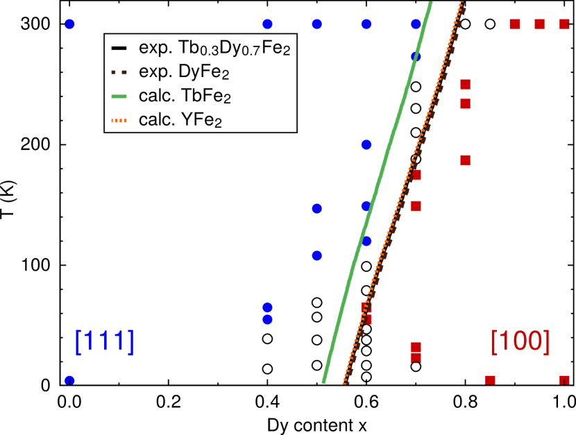
Figure 4: The spin orientation diagram of Tb_1-xDy_xFe₂ calculated with different sets of elastic constants. The same experimental data is shown as in Fig. 3. The diagonal lines represent the boundaries between [111] and [100] directions of magnetization for the different sets of elastic constants listed in Table 2.

We recalculated the spin orientation diagram for each set of constants and show the result in Fig. 4. The qualitative structure of the diagram for each set of constants is identical, consisting of a single boundary between [111] and [100] easy directions. Quantitatively, the three sets of elastic constants corresponding to Tb_0.3Dy_0.7Fe₂ and DyFe₂ (experimental) and YFe₂ Bentouaf et al. (2016); Moulay et al. (2013) (calculated) give effectively identical boundaries. Using the elastic constants calculated for TbFe₂ shifts the critical concentration $x_{c}$ down by approximately 0.05, such that $x_{c}=0.51$ at 0 K and $x_{c}=0.72$ at 300 K. Examining Table 2 would indicate that the critical concentration is most sensitive to $c_{44}$, which is reasonable given crucial role played by the large [111] magnetostriction.

We note that using the elastic constants calculated for TbFe₂ brings the room temperature critical concentration to within 0.01 of the experimental Terfenol-D value. However, since it is not clear that a GGA treatment is sufficiently accurate to describe the Tb-4$f$ electrons Bentouaf et al. (2016); Patrick and Staunton (2018), in this work we prefer to use experimental values for the elastic constants. Furthermore, the effectively identical results for Tb_0.3Dy_0.7Fe₂ and DyFe₂, and the weak sensitivity to $c_{ij}$ in general, justifies the use of a single set of elastic constants for the entire spin orientation diagram.

References

- Abbundi and Clark (1977) R. Abbundi and A. Clark, Anomalous thermal expansion and magnetostriction of single crystal Tb.27Dy.73Fe2, IEEE Trans. Magn. 13, 1519 (1977).
- Clark (1973) A. E. Clark, High-field magnetization and coercivity of amorphous rare-earth-Fe2 alloys, Appl. Phys. Lett. 23, 642 (1973).
- Clark et al. (1977) A. Clark, R. Abbundi, H. Savage, and O. McMasters, Magnetostriction of rare earth-Fe2 Laves phase compounds, Physica B+C 86-88, 73 (1977).
- du Trémolet de Lacheisserie (1993) E. du Trémolet de Lacheisserie, Magnetostriction: Theory and Applications of Magnetoelasticity (CRC Press, 1993).
- Staley and Flatau (2005) M. E. Staley and A. B. Flatau, Characterization of energy harvesting potential of Terfenol-D and Galfenol, in Smart Structures and Materials 2005: Smart Structures and Integrated Systems, Vol. 5764, edited by A. B. Flatau, International Society for Optics and Photonics (SPIE, 2005) pp. 630 – 640.
- Deng and Dapino (2017) Z. Deng and M. J. Dapino, Review of magnetostrictive vibration energy harvesters, Smart Mater. Struct. 26, 103001 (2017).
- Rudd and Myers (2018) J. Rudd and O. Myers, Experimental fabrication and nondestructive testing of carbon fiber beams for delaminations using embedded Terfenol-D particles, J. Intel. Mat. Syst. Str. 29, 600 (2018).
- Wang et al. (2017) Q. Wang, X. Li, C.-Y. Liang, A. Barra, J. Domann, C. Lynch, A. Sepulveda, and G. Carman, Strain-mediated 180∘ switching in CoFeB and Terfenol-D nanodots with perpendicular magnetic anisotropy, Appl. Phys. Lett. 110, 102903 (2017).
- Li et al. (2018) D. Li, X.-M. Zhao, H.-X. Zhao, X.-W. Dong, L.-S. Long, and L.-S. Zheng, Construction of Magnetoelectric Composites with a Large Room-Temperature Magnetoelectric Response through Molecular-Ionic Ferroelectrics, Advanced Materials 30, 1803716 (2018).
- Atulasimha and Flatau (2011) J. Atulasimha and A. B. Flatau, A review of magnetostrictive iron–gallium alloys, Smart Mater. and Struct. 20, 043001 (2011).
- Vincent et al. (2020) J. D. S. Vincent, M. Rodrigues, Z. Leong, and N. A. Morley, Design and Development of Magnetostrictive Actuators and Sensors for Structural Health Monitoring, Sensors 20, 711 (2020).
- Clark et al. (2003) A. E. Clark, K. B. Hathaway, M. Wun-Fogle, J. B. Restorff, T. A. Lograsso, V. M. Keppens, G. Petculescu, and R. A. Taylor, Extraordinary magnetoelasticity and lattice softening in bcc Fe-Ga alloys, J. Appl. Phys. 93, 8621 (2003).
- Clark et al. (2008) A. E. Clark, J. B. Restorff, M. Wun-Fogle, D. Wu, and T. A. Lograsso, Temperature dependence of the magnetostriction and magnetoelastic coupling in Fe100-xAlx (=14.1,16.6,21.5,26.3) and Fe50Co50, J. Appl. Phys. 103, 07B310 (2008).
- Brooks et al. (1991) M. S. S. Brooks, L. Nordström, and B. Johansson, 3d-5d band magnetism in rare earth-transition metal intermetallics: total and partial magnetic moments of the RFe2 (R=Gd-Yb) Laves phase compounds, J. Phys.: Condens. Matter 3, 2357 (1991).
- Richter (1998) M. Richter, Band structure theory of magnetism in 3d-4f compounds, J. Phys. D: Appl. Phys. 31, 1017 (1998).
- Buck and Fähnle (1999) S. Buck and M. Fähnle, Magnetostriction in TbFe2: weak influence of the internal structural distortion, J. Magn. Magn. Mater. 204, L1 (1999).
- Gavrilenko and Wu (2001) V. I. Gavrilenko and R. Q. Wu, Magnetostriction and magnetism of rare earth intermetallic compounds: First principle study, J. Appl. Phys. 89, 7320 (2001).
- Fähnle and Welsch (2002) M. Fähnle and F. Welsch, From the electronic structure to the macroscopic magnetic behaviour of rare-earth intermetallics: a combination of ab initio electron theory with statistical mechanics and elasticity theory, Physica B: Condens. Matt. 321, 198 (2002).
- Wang et al. (2013) H. Wang, Y. N. Zhang, R. Q. Wu, L. Z. Sun, D. S. Xu, and Z. D. Zhang, Understanding strong magnetostriction in Fe100-xGax alloys, Sci. Rep. 3, 3521 (2013).
- Atzmony et al. (1973) U. Atzmony, M. P. Dariel, E. R. Bauminger, D. Lebenbaum, I. Nowik, and S. Ofer, Spin-Orientation Diagrams and Magnetic Anisotropy of Rare-Earth-Iron Ternary Cubic Laves Compounds, Phys. Rev. B 7, 4220 (1973).
- Koon and Williams (1978) N. C. Koon and C. M. Williams, Origins of magnetic anisotropy in cubic RFe2 Laves phase compounds, J. Appl. Phys. 49, 1948 (1978).
- Kuz’min (2001) M. D. Kuz’min, Magnetostriction of DyFe2 and HoFe2: Validity of the single-ion model, J. Appl. Phys. 89, 5592 (2001).
- Bowden et al. (2004) G. J. Bowden, P. A. J. de Groot, J. D. O’Neil, B. D. Rainford, and A. A. Zhukov, On the anomalous temperature-dependent magnetostriction in intermetallic DyFe2, J. Phys. Condens. Matter 16, 2437 (2004).
- Martin et al. (2006) K. N. Martin, P. A. J. de Groot, B. D. Rainford, K. Wang, G. J. Bowden, J. P. Zimmermann, and H. Fangohr, Magnetic anisotropy in the cubic Laves REFe2 intermetallic compounds, J. Phys.: Condens. Matter 18, 459 (2006).
- Patrick and Staunton (2019a) C. E. Patrick and J. B. Staunton, Crystal field coefficients for yttrium analogues of rare-earth/transition-metal magnets using density-functional theory in the projector-augmented wave formalism, J. Phys.: Condens. Matter 31, 305901 (2019a).
- Clark (1980) A. Clark, Magnetostrictive Rare Earth-Fe2 Compounds, in Handbook of Ferromagnetic Materials, Vol. 1 (Elsevier, 1980) p. 531.
- Györffy et al. (1985) B. L. Györffy, A. J. Pindor, J. Staunton, G. M. Stocks, and H. Winter, A first-principles theory of ferromagnetic phase transitions in metals, J. Phys. F: Met. Phys. 15, 1337 (1985).
- Note (1) We note that in a ferrimagnet like REFe2, the itinerant electron magnetic sublattice may be oriented antiparallel to ; however this detail does not affect our discussion, since .
- Kittel (1949) C. Kittel, Physical theory of ferromagnetic domains, Rev. Mod. Phys. 21, 541 (1949).
- Bentouaf et al. (2016) A. Bentouaf, R. Mebsout, H. Rached, S. Amari, A. Reshak, and B. Aïssa, Theoretical investigation of the structural, electronic, magnetic and elastic properties of binary cubic C15-Laves phases TbX2 (X = Co and Fe), J. Alloys Compd. 689, 885 (2016).
- Moulay et al. (2013) N. Moulay, H. Rached, M. Rabah, S. Benalia, D. Rached, A. H. Reshak, N. Benkhettou, and P. Ruterana, First-principles calculations of the elastic, and electronic properties of YFe2, NiFe2 and YNiFe4 intermetallic compounds, Comp. Mater. Sci. 73, 56 (2013).
- Kuz’min and Tishin (2008) M. D. Kuz’min and A. M. Tishin, Theory of Crystal-Field Effects in 3-4 Intermetallic Compounds, in Handbook of Magnetic Materials, Vol. 17 (Elsevier, 2008) p. 149.
- Marchant et al. (2019) G. A. Marchant, C. E. Patrick, and J. B. Staunton, Ab initio calculations of temperature-dependent magnetostriction of Fe and 2 Fe1-xGax within the disordered local moment picture, Phys. Rev. B 99, 054415 (2019).
- Callen and Callen (1966) H. Callen and E. Callen, The present status of the temperature dependence of magnetocrystalline anisotropy, and the power law, J. Phys. Chem. Solids 27, 1271 (1966).
- Loewenhaupt et al. (1996) M. Loewenhaupt, P. Tils, K. Buschow, and R. Eccleston, Exchange interactions in GdFe compounds studied by inelastic neutron scattering, J. Magn. Magn. Mater. 152, 10 (1996).
- Griffith (1961) J. S. Griffith, The Theory of Transition-Metal Ions (Cambridge University Press, 1961).
- Patrick and Staunton (2019b) C. E. Patrick and J. B. Staunton, Temperature-dependent magnetocrystalline anisotropy of rare earth/transition metal permanent magnets from first principles: The light Co5 intermetallics, Phys. Rev. Materials 3, 101401 (2019b).
- Sievers (1982) J. Sievers, Asphericity of 4-shells in their Hund’s rule ground states, Z. Phys. B 45, 289 (1982).
- Stevens (1952) K. W. H. Stevens, Matrix Elements and Operator Equivalents Connected with the Magnetic Properties of Rare Earth Ions, Proc. Phys. Soc. A 65, 209 (1952).
- Edmonds (1960) A. R. Edmonds, Angular momentum in quantum mechanics (Princeton University Press, Princeton, New Jersey, 1960) Chap. 4, p. 59.
- Bradley and Cracknell (1972) C. J. Bradley and A. P. Cracknell, The Mathematical Theory of Symmetry in Solids (Oxford University Press, 1972) Chap. 3, p. 82.
- Kumar et al. (2020a) S. Kumar, C. E. Patrick, R. S. Edwards, G. Balakrishnan, M. R. Lees, and J. B. Staunton, Torque magnetometry study of the spin reorientation transition and temperature-dependent magnetocrystalline anisotropy in NdCo5, J. Phys.: Condens. Matter 32, 255802 (2020a).
- Kumar et al. (2020b) S. Kumar, C. E. Patrick, R. S. Edwards, G. Balakrishnan, M. R. Lees, and J. B. Staunton, Tunability of the spin reorientation transitions with pressure in NdCo5, Appl. Phys. Lett. 116, 102408 (2020b).
- Lüders et al. (2005) M. Lüders, A. Ernst, M. Däne, Z. Szotek, A. Svane, D. Ködderitzsch, W. Hergert, B. L. Györffy, and W. M. Temmerman, Self-interaction correction in multiple scattering theory, Phys. Rev. B 71, 205109 (2005).
- Däne et al. (2009) M. Däne, M. Lüders, A. Ernst, D. Ködderitzsch, W. M. Temmerman, Z. Szotek, and W. Hergert, Self-interaction correction in multiple scattering theory: application to transition metal oxides, J. Phys. Condens. Matter 21, 045604 (2009).
- Note (2) These functions were reported previously in Ref. Patrick and Staunton (2019a), Fig. 1 and are available on request.
- Patrick et al. (2018) C. E. Patrick, S. Kumar, G. Balakrishnan, R. S. Edwards, M. R. Lees, L. Petit, and J. B. Staunton, Calculating the Magnetic Anisotropy of Rare-Earth/Transition-Metal Ferrimagnets, Phys. Rev. Lett. 120, 097202 (2018).
- Patrick and Staunton (2018) C. E. Patrick and J. B. Staunton, Rare-earth/transition-metal magnets at finite temperature: Self-interaction-corrected relativistic density functional theory in the disordered local moment picture, Phys. Rev. B 97, 224415 (2018).
- Staunton et al. (2006) J. B. Staunton, L. Szunyogh, A. Buruzs, B. L. Gyorffy, S. Ostanin, and L. Udvardi, Temperature dependence of magnetic anisotropy: An ab initio approach, Phys. Rev. B 74, 144411 (2006).
- Patrick et al. (2017) C. E. Patrick, S. Kumar, G. Balakrishnan, R. S. Edwards, M. R. Lees, E. Mendive-Tapia, L. Petit, and J. B. Staunton, Rare-earth/transition-metal magnetic interactions in pristine and (Ni,Fe)-doped and , Phys. Rev. Materials 1, 024411 (2017).
- Györffy and Stocks (1979) B. L. Györffy and G. M. Stocks, First principles band theory for random metallic alloys, in Electrons in Disordered Metals and at Metallic Surfaces, Nato Science Series B, edited by P. Phariseau and B. Györffy (Springer US, 1979) Chap. 4, pp. 89–192.
- Enkovaara et al. (2010) J. Enkovaara, C. Rostgaard, J. J. Mortensen, J. Chen, M. Dułak, L. Ferrighi, J. Gavnholt, C. Glinsvad, V. Haikola, H. A. Hansen, et al., Electronic structure calculations with GPAW: a real-space implementation of the projector augmented-wave method, J. Phys. Condens. Matter 22, 253202 (2010).
- Vosko et al. (1980) S. H. Vosko, L. Wilk, and M. Nusair, Accurate spin-dependent electron liquid correlation energies for local spin density calculations: a critical analysis, Can. J. Phys. 58, 1200 (1980).
- Andreev (1995) A. V. Andreev, Thermal expansion anomalies and spontaneous magnetostriction in rare-earth intermetallics with cobalt and iron, in Handbook of Magnetic Materials, Vol. 8, edited by K. H. J. Buschow (Elsevier North-Holland, New York, 1995) Chap. 2, p. 59.
- Wedler et al. (2000) G. Wedler, J. Walz, A. Greuer, and R. Koch, The magnetoelastic coupling constant of epitaxial Fe(001) films, Surf. Sci. 454-456, 896 (2000).
- Atzmony et al. (1977) U. Atzmony, M. P. Dariel, and G. Dublon, Spin-orientation diagram of the pseudobinary Tb1-xDyxFe2 Laves compounds, Phys. Rev. B 15, 3565 (1977).
- Williams et al. (1980) C. Williams, N. Koon, and B. Das, Torque measurements on single crystal DyxTb1-xFe2 compounds, J. Magn. Magn. Mater. 15-18, 553 (1980).
- Atzmony and Dariel (1976) U. Atzmony and M. P. Dariel, Nonmajor cubic symmetry axes of easy magnetization in rare-earth-iron Laves compounds, Phys. Rev. B 13, 4006 (1976).
- Cullen and Clark (1977) J. R. Cullen and A. E. Clark, Magnetostriction and structural distortion in rare-earth intermetallics, Phys. Rev. B 15, 4510 (1977).