TOWARD RELIABLE MODELS FOR AUTHENTICATING MULTIMEDIA CONTENT: DETECTING RESAMPLING ARTIFACTS WITH BAYESIAN NEURAL NETWORKS

Abstract

In multimedia forensics, learning-based methods provide state-of-the-art performance in determining origin and authenticity of images and videos. However, most existing methods are challenged by out-of-distribution data, i.e., with characteristics that are not covered in the training set. This makes it difficult to know when to trust a model, particularly for practitioners with limited technical background.

In this work, we make a first step toward redesigning forensic algorithms with a strong focus on reliability. To this end, we propose to use Bayesian neural networks (BNN), which combine the power of deep neural networks with the rigorous probabilistic formulation of a Bayesian framework. Instead of providing a point estimate like standard neural networks, BNNs provide distributions that express both the estimate and also an uncertainty range.

We demonstrate the usefulness of this framework on a classical forensic task: resampling detection. The BNN yields state-of-the-art detection performance, plus excellent capabilities for detecting out-of-distribution samples. This is demonstrated for three pathologic issues in resampling detection, namely unseen resampling factors, unseen JPEG compression, and unseen resampling algorithms. We hope that this proposal spurs further research toward reliability in multimedia forensics.

Index Terms—  digital image forensics, reliability, Bayesian neural networks, resampling detection

1 Introduction

The goal of image forensics is to validate origin and authenticity of digital images. Most state-of-the-art forensic methods are based on deep learning. Notable example applications are to blindly validate noise statistics [1], to link EXIF tags to noise statistics [2], to detect artifacts of commonly used operators [3, 4], to detect computer-generated imagery [5, 6], or to detect JPEG inconsistencies [7].

The success of learning-based methods can broadly be attributed to their excellent capability in deriving most subtle cues from training examples. However, one notable disadvantage of learning-based methods is their sensitivity to out-of-distribution data: if a test image differs too much from the training dataset, learning-based methods oftentimes exhibit difficulties in detecting these cues [8].

Such out-of-distribution scenarios are, unfortunately, quite common in the practical forensic work: oftentimes, little is known about the exact provenance of an image, particularly when it was found on the internet. For example, there may be only limited knowledge about the type and amount of in-camera processing that an image underwent, and limited knowledge about distribution-related postprocessing such as the implementation of the JPEG library of a web platform. Current forensic methods address this issue with extensive data augmentation [1, 2, 5, 6]. The aim of such data augmentation is to anticipate a rich variety of commonly seen processing steps and compression variants to harden the network against variations of the input data.

However, although current methods achieve impressive results on a wide variety of inputs, augmentation can only extend the horizon of seen data. It does not provide knowledge about potential failure cases from unseen data. This can be a severe practical limitation: a forensic analyst has to understand on which data a method can operate or not in order to assess its output.

In this work, we propose a different direction to mitigate this issue: The first contribution is to propose Bayesian neural networks (BNNs) for image forensics to intrinsically model uncertainty about the data. BNNs combine the strengths of deep neural networks with a rigorous probabilistic framework. Thus, BNNs are also amenable to data augmentation to increase the range of seen data, but they can also detect whenever operating on unseen data. This enables an analyst to know about network uncertainty without requiring expertise in the technical specifics.

The second contribution is to demonstrate the usefulness of the proposed approach on a classical forensic task, namely the detection of resampling. The proposed BNN achieves state-of-the-art detection performance. Additionally, it shows impressive capabilities to detect out-of-distribution inputs on three notorious issues in resampling detection, namely previously unseen rescaling ranges, JPEG postcompression, and rescaling algorithms.

This paper is organized as follows. In Sec. 2, we describe related work on uncertainty modeling in neural networks and on resampling detection. Section 3 introduces the basic concepts of the Bayesian framework for convolutional neural networks (CNNs) and variational inference. Section 4 presents experimental results on various resampling scenarios. Section 5 concludes with a brief summary and outlook.

2 Related Work

Detecting out-of-distribution examples has recently gained popularity in the machine learning community. Hendrycks and Gimpel proposed the softmax activations of a neural network to anticipate incorrect classifications and detect out-of-distribution samples [9]. However, the usefulness of softmax statistics is limited. Guo et al. show that these softmax probabilities do not accurately represent the “true correctness likelihood” [10]. Liang et al. [11] propose to calibrate softmax activations to the model confidence via temperature scaling and input preprocessing similar to the fast gradient sign method introduced by [12]. This approach results in a local distillation of the input space, but it does not solve the general problems that neural networks make confident errors and do not provide information of their predictive uncertainty. To address these issues, DeVries and Taylor [13] propose to learn confidence estimates by training a network with two output branches producing prediction and uncertainty estimate.

Similar goals to model uncertainty can be achieved with a Bayesian framework, which has a more solid theoretical foundation. Gal and Ghahramani [14] show how Bayesian inference can be approximated with standard CNNs using dropout at test time. Inspired by their approach, Lakshminarayanan et al. [15] use an ensemble of networks to obtain uncertainty estimates. Both works, however, do not model the full posterior distribution but are a discrete approximation of the Bayesian approach.

Blundell et al. [16] show that Bayesian methods can be applied to neural networks to model probability distributions over the trainable weights instead of point estimates. This property enables the network to predict uncertainty based on which the analyst can choose whether or not to trust the model’s prediction. Bayesian neural networks have demonstrated impressive results in various tasks, e.g., pixel-wise depth regression [17], biomedical image segmentation [18]. We argue that this framework is also particularly well suited for the field of forensics.

We demonstrate the usefulness of the Bayesian framework on the classical forensic task of resampling detection. In resampling detection, the assumption is that when an object is spliced into an image, it is likely resized or rotated to fit into the target scene. Algorithmically, resizing or rotation is typically implemented as a resampling operation. In the past 15 years, many analytic forensic techniques were proposed to detect resampling, e.g., via quasi-periodic inter-pixel correlations [19], random matrix theory [20], or natural image statistics [21].

Several learning-based methods achieve similar goals, either by directly detecting resampling [22] or the resampling factor [23], or indirectly via camera-based image forgery localization [24] or the detection of image splicing [25]. However, learning-based methods are sensitive to mismatches between training and test data. For example, Liu and Kirchner report that their CNN for rescaling factor estimation suffers from poor generalization to unseen resampling algorithms like bicubic interpolation [23]. They also report that including more diverse training examples lead to a reduction in the overall accuracy. Moreover, it is certainly intractable to cover all possible real-world scenarios in the training data.

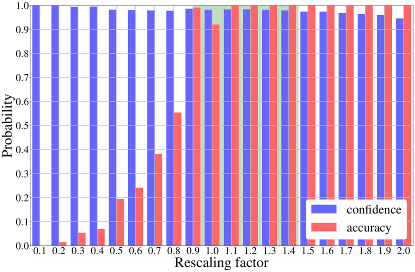
Fig. 1: Baseline CNN: prediction confidence (blue) versus accuracy (red), averaged over $128$ samples for scaling factors from $0.1$ to $2.0$ with step size $0.1$ (see text for details).

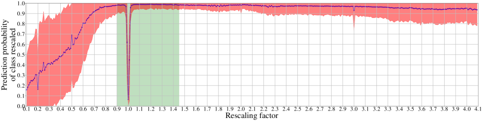
Fig. 2: Uncertainty of the Bayesian CNN. Blue: prediction probability for “rescaled”, averaged over 128 input samples. Red: two standard deviations from the mean, calculated from $50$ Monte Carlo draws from the posterior probability. Green: scaling factors for network training.

3 Bayesian Nets and Variational Inference

Standard neural networks can be seen as universal function approximators, able to represent an arbitrary function $G(\boldsymbol{x})$ within an arbitrary small but fixed distance $\varepsilon$ by a learned function $g_{\boldsymbol{\omega}}(\boldsymbol{x})$,

$$|G(\boldsymbol{x})-g_{\boldsymbol{\omega}}(\boldsymbol{x})|<\varepsilon\enspace.$$ (1)

Here, $\boldsymbol{\omega}\in\rm I\!R^{t}$ denotes the $t$ trainable network parameters or weights. Training is usually formulated as an optimization problem, and solved for the optimal weights $\boldsymbol{\omega}$ via gradient descent. These weights are scalar quantities and hence form a point estimate. Standard neural networks can learn powerful representations. However, they also suffer from overly confident decisions on unseen data. Moreover, these models are by design deterministic, and as such not able to express uncertainty in their decisions.

The BNN does not learn point estimates, but instead the posterior distribution $P(\boldsymbol{\omega}|\mathcal{D})$ over the weights $\boldsymbol{\omega}$ given some training data $\mathcal{D}=\{\left(\boldsymbol{x}_{i},\boldsymbol{y}_{i}\right)\},\;i=1\dots S$. Here, $S$ is the number of training samples, and the samples are tuples of input images $\boldsymbol{x}_{i}$ and their corresponding class label $\boldsymbol{y}_{i}$ that follows a categorical distribution. Exact Bayesian inference, i.e., the exact calculation of the posterior, is intractable due to the large number of parameters in a neural network. Blundell et al. [16] introduced the Bayes by Backprop algorithm, which approaches a variational approximation of the posterior distribution. It enables to learn a probability distribution over the trainable weights in a network.

Variational learning aims to find optimal parameters $\theta$ of the weight distribution $q(\boldsymbol{\omega}|\theta)$, which is achieved when $q(\boldsymbol{\omega}|\theta)$ is similar to the true unknown distribution $P(\boldsymbol{\omega}|\mathcal{D})$. This corresponds to minimizing the Kullback-Leibler divergence

$$\theta^{\ast} =\mathop{\operator@font argmin}_{\theta}KL\left[q(\boldsymbol{\omega}|\theta)||P(\boldsymbol{\omega}|\mathcal{D})\right]$$ (2)

$$=\mathop{\operator@font argmin}_{\theta}\int q(\boldsymbol{\omega}|\theta)\log{\frac{q(\boldsymbol{\omega}|\theta)}{P(\boldsymbol{\omega}|\mathcal{D})}}d\boldsymbol{\omega}$$

$$=\mathop{\operator@font argmin}_{\theta}\int q(\boldsymbol{\omega}|\theta)\log{\frac{q(\boldsymbol{\omega}|\theta)}{P(\boldsymbol{\omega})P(\mathcal{D}|\boldsymbol{\omega})}}d\boldsymbol{\omega}$$

$$=\mathop{\operator@font argmin}_{\theta}\int q(\boldsymbol{\omega}|\theta)\log{\frac{q(\boldsymbol{\omega}|\theta)}{P(\boldsymbol{\omega})}}-q(\boldsymbol{\omega}|\theta)\log{P(\mathcal{D}|\boldsymbol{\omega})}d\boldsymbol{\omega}$$

$$=\mathop{\operator@font argmin}_{\theta}\int q(\boldsymbol{\omega}|\theta)\log{\frac{q(\boldsymbol{\omega}|\theta)}{P(\boldsymbol{\omega})}}d\boldsymbol{\omega}-\int q(\boldsymbol{\omega}|\theta)\log{P(\mathcal{D}|\boldsymbol{\omega})}d\boldsymbol{\omega}$$

$$=\mathop{\operator@font argmin}_{\theta}KL\left[q(\boldsymbol{\omega}|\theta)||P(\boldsymbol{\omega})\right]-\mathord{\rm I\!E}_{q(\boldsymbol{\omega}|\theta)}\left[\log{P(\mathcal{D}|\boldsymbol{\omega})}\right]\enspace.$$

In the last equation, the second term denotes the negative log-likelihood, which is usually optimized via maximum likelihood estimation (MLE). The first term acts as regularizer in a maximum a posteriori (MAP) sense. Overall, Eqn. 2 minimizes the negative log-likelihood while enforcing a small Kullback-Leibler divergence between the weight distribution and the prior distribution. This cost function is known as the evidence lower bound (elbo) loss. Direct optimization of this cost function is computationally expensive. However, it can be approximated as a function of the training data $\mathcal{D}$ and the variational parameters $\theta$ via gradient descent and the dominated convergence theorem, which allows to interchange a derivative with an expectation. This allows to rewrite the optimization problem in Eqn. 2 to

$$f(\boldsymbol{\omega},\theta)=\log{q(\boldsymbol{\omega}|\theta)}-\log{P(\boldsymbol{\omega})}-\log{P(\mathcal{D}|\boldsymbol{\omega})}\enspace.$$ (3)

The exact cost then can be approximated as

$$\mathcal{F}(\mathcal{D},\theta)\approx\sum_{i=1}^{n}\log q(\boldsymbol{\omega}^{i}|\theta)-\log P(\boldsymbol{\omega}^{i})-\log P(\mathcal{D}|\boldsymbol{\omega}^{i})\enspace,$$ (4)

where $\boldsymbol{\omega}^{i}$ denotes the $i$-th sample drawn from the variational posterior. The Bayes by Backprop algorithm introduced by Blundell et al. [16] was formulated for feed-forward neural networks using fully connected layers. Their approach can be generalized to convolutional neural networks by applying flipout convolution [26]. This enables the estimation of the predictive posterior via sampling from the variational posterior, similar to [18],

$$\mathord{\rm I\!E}_{q(\boldsymbol{\omega}|\theta)}\left[P(\boldsymbol{y}^{*}|\boldsymbol{x}^{*})\right] =\int P(\boldsymbol{y}^{*}|\boldsymbol{x}^{*},\boldsymbol{\omega})q(\boldsymbol{\omega}|\theta)d\boldsymbol{\omega}$$ (5)

$$\approx\frac{1}{n}\sum_{i=1}^{n}P_{\boldsymbol{\omega}^{i}}(\boldsymbol{y}^{*}|\boldsymbol{x}^{*})\enspace,$$ (6)

where $\boldsymbol{x}^{*}$ denotes unseen data, $\boldsymbol{y}^{*}$ the predicted class label and $P_{\boldsymbol{\omega}^{i}}(\boldsymbol{y^{*}}|\boldsymbol{x}^{*})$ a draw from the predictive posterior. The approximation in Eqn. 6 samples $n$ times from the trained network on unseen data. The variance of this estimator expresses the network’s uncertainty in its prediction [18],

$$\mathrm{Var}(P(\boldsymbol{y}|\boldsymbol{x}))=\mathord{\rm I\!E}_{q(\boldsymbol{\omega}|\theta)}[\boldsymbol{y}\boldsymbol{y}^{T}]-\mathord{\rm I\!E}_{q(\boldsymbol{\omega}|\theta)}[\boldsymbol{y}]\mathord{\rm I\!E}_{q(\boldsymbol{\omega}|\theta)}[\boldsymbol{y}]^{T}\enspace.$$ (7)

4 Experimental results

We conduct a series of experiments on rescaling detection to evaluate the robustness of the Bayesian CNN (BNN) and its ability to express predictive uncertainty.

Dataset Preparation. We randomly select 1 000 uncompressed high-resolution images from the RAISE dataset [27]. Each RGB color image is converted to grayscale using the ITU-R 601-2 luma transform. The 1 000 images are split into 800 images for training, 100 images for validation, and 100 images for testing. Each image is further processed as follows: one copy is left as original, and one copy is rescaled with a rescaling factor $s=0.9+k\cdot 0.05$, where $k$ is randomly chosen between $0$ and $11$ excluding $2$, i.e., scaling factors are between $0.9$ and $1.45$ excluding the identity $1.00$. From both copies we randomly draw $N=50$ non-overlapping patches of $256\times 256$ pixels. Hence, training, validation, and testing sets consist of 80 000, 10 000, and 10 000 patches from disjunct images.

Network Architectures. As a baseline, we use the popular constrained convolutional architecture by Bayar and Stamm [28]. We implement this architecture in Tensorflow, but omit the extremely randomized trees classifier in order to perform a frictionless comparison of end-to-end deep learning architectures.

The Bayesian network uses the baseline network as template, with the same number of layers, same number and dimensions of the filter kernels per convolution layer, and the same constrained convolution layer. The Bayesian property is obtained via flipout convolution and fully-connected layers [26] from the Tensorflow probability framework [29]. As prior distribution we assume a zero-mean Gaussian distribution with unit-variance. For inference, we use Eqn. 6 with $n=50$ Monte Carlo draws, and we calculate the predictive variance via Eqn. 7. We assume a normally-distributed variational posterior, hence the Bayesian network has twice as many training parameters as the baseline CNN.

Training Parameters We use the Adam optimizer with a learning rate of $l=10^{-3}$, $\beta_{1}=0.9$, $\beta_{2}=0.999$ and $\epsilon=10^{-7}$, and a batch size of $64$. The baseline is trained for 100 000 iterations. The BNN for 150 000 iterations due to twice the network parameters. The reported results use the model that best performs on the validation set, which is evaluated every 1 000 iterations.

4.1 Detection Accuracy

The baseline model and the Bayesian CNN are trained for the detection of rescaling using the same datasets and hyper-parameters. On the test set, the baseline achieves $96.32\%$ accuracy. This is comparable to [28] given that the additional extremely randomised trees for performance boosting are omitted. The Bayesian CNN achieves $97.40\%$ accuracy, which is comparable, even slightly better.

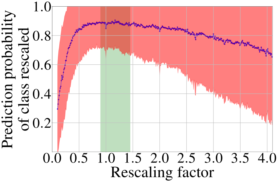
(a) JPEG-compression ($q=85$)

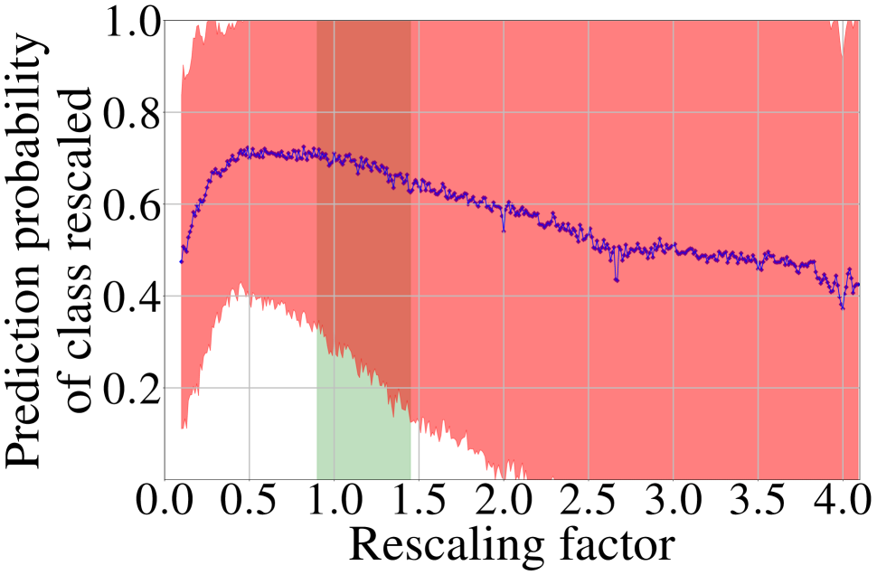
(b) JPEG-compression ($q=50$)

Fig. 3: Uncertainty by the Bayesian CNN on out-of-distribution test samples with JPEG postcompression.

4.2 Standard CNN and Out-of-Distribution Samples

We first show that a standard CNN does not provide helpful information to detect out-of-distribution samples. To this end, recall that the baseline CNN is trained on resampling factors in the range of $s\in\{0.9\dots 1.45\}$. For testing, we create a second test set with resampling factors $s^{\prime}=\{0.1\dots 2.0\}$ in steps of $0.1$. With exception of the resampling range, the test set preparation follows the exact same protocol as the previous dataset. In particular, the test images are unseen during network training. We select $M=128$ patches per rescaling factor, and calculate average accuracy and confidence per rescaling factor. The confidence is calculated as [9]

$$c_{s}=\frac{1}{M}\sum_{m=1}^{M}\max_{y_{k}}P(y_{k}\mid\boldsymbol{x}_{m})\enspace,$$ (8)

i.e., averaging the highest activation per decision per rescaling factor.

The results are shown in Fig. 1. The rescaling factors $0.1$ to $2.0$ are on the $x$-axis. The range of rescaling factors for network training is shown in green. Red bars indicate the accuracy of the baseline method per rescaling factor $s$. Blue bars indicate the associated confidence $c_{s}$. It can be observed that the blue confidence bars are always very high, at or beyond $0.9$. Moreover, the confidence is independent of the actual network accuracy, which significantly varies across resampling factors. This makes it impossible to predict the network performance from the distribution of class activations.

4.3 Uncertainty in Out-of-Distribution Resampling Factors

The previous experiment is repeated with the BNN. To this end, we expand the range of rescaling factors even further to $[0.1;4.1]$ with step size $0.01$, and leave all other experimental parameters identical.

The results are shown in Fig. 2. Green indicates the range of training data. The blue line shows the mean prediction probability for “rescaled”, averaged over $M=128$ randomly selected patches. Red indicates two standard deviations of the uncertainty. The network excellently performs inside the train region, distinguishing the original and rescaled patches with over $99\%$ confidence, while exhibiting very low uncertainty in its decision. The network generalizes very well for scaling factors $s\geq 1.5$. With increasing distance to the training region, the uncertainty grows accordingly with a slight reduction in accuracy, which is the desired behavior. For downscaling, the network is able to detect scaling factors $s\geq 0.7$, i.e., in direct proximity to the train region. For scaling factors $s<0.7$, the network prediction performance drops considerably, and the uncertainty again grows accordingly. Hence, the network uncertainty indicates its inability to operate on this input. We consider this an important cue for a forensic analyst to not trust the network output.

Both networks, the baseline in Fig. 1 and the Bayesian CNN in Fig. 2, make errors on out-of-distribution examples. However, where the standard CNN makes extremely overconfident errors, the Bayesian CNN tends to be uncertain, which can inform the analyst whether she can trust the network prediction or not.

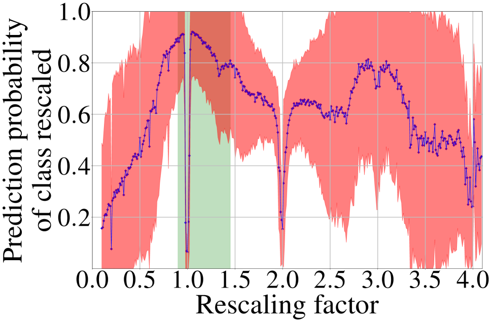
(a) nearest-neighbor interpolation

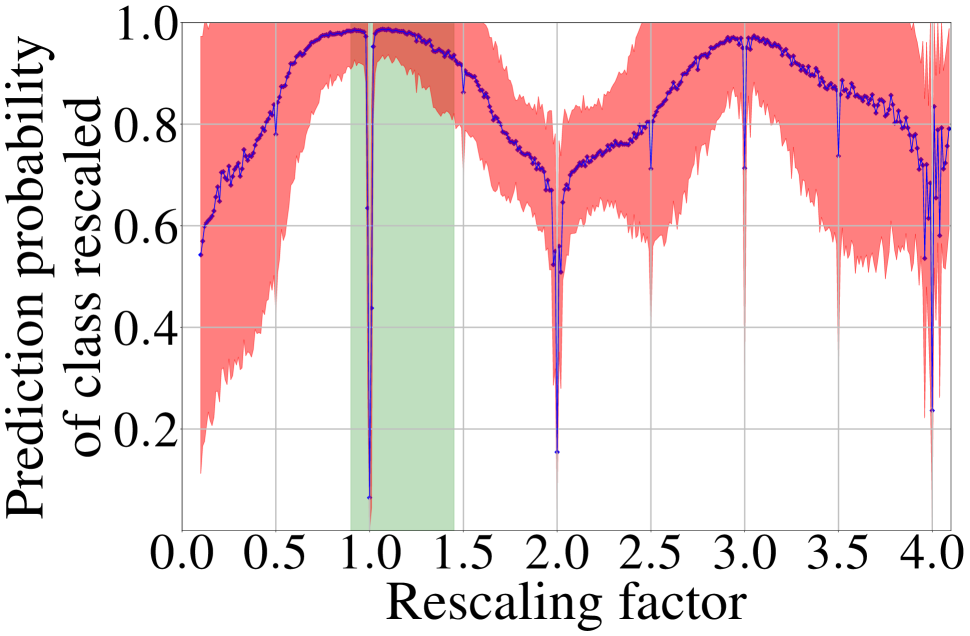
(b) areal interpolation

Fig. 4: Uncertainty by the Bayesian CNN on out-of-distribution test samples of nearest-neighbor and areal interpolation.

4.4 Uncertainty in Out-of-Distribution JPEG Compression

There are numerous scenarios that might not be well covered in the classifier training set. We select two cases, namely unseen resampling methods and JPEG compression after resampling.

Data augmentation with JPEG compression is routinely performed in many forensic algorithms. Nevertheless, we believe that JPEG compression is an interesting experiment, for it is widely accepted in the forensic community as a prototypic case for out-of-distribution samples: since the BNN training data is uncompressed, we can observe how the BNN uncertainty serves as a metric for the network prediction reliability. In this experiment, we recompress all testing data with quality factors $q=85$ and $q=50$. The remaining experimental protocol is identical to the previous sections.

The results of this experiment are shown in Fig. 3. As expected, the prediction probability drops with increasing compression and with increasing deviation from the training resampling parameters. It is encouraging to observe that this is accurately indicated by a simultaneous increase in the uncertainty.

4.5 Uncertainty in Out-of-Distribution Resampling Operations

A more subtle case of out-of-distribution samples are variations in the resampling operations. Such deviations in the data distribution are much more difficult to catch, and might even be non-obvious to a technical expert. In this experiment, we use nearest neighbor interpolation and an areal interpolation on the testing data. The remaining experimental protocol is identical to the previous sections.

The results of this experiment are shown in Fig. 4. Analogous to the JPEG experiments, prediction probabilities are also significantly lower, but the uncertainty increase accordingly, which again makes it possible to detect the mismatch between training and testing data.

5 Conclusion

We propose a novel Bayesian deep learning approach to express predictive uncertainty in image forensics. We show on the example of resampling detection that the Bayesian CNN avoids confident errors. Moreover, the Bayesian framework intrinsically provides an uncertainty estimate that indicates a model mismatch to a forensic analyst, which is otherwise difficult to recognize.

This is preliminary work. We believe that BNNs can close an important gap in image forensics, but there are still many aspects to be investigated. In future work, we will extend this approach to other forensic tasks, explore selection strategies for prior distributions, and explore a decomposition of the predictive uncertainty into model and data uncertainty [18].

References

- [1] D. Cozzolino and L. Verdoliva, “Noiseprint: a cnn-based camera model fingerprint,” IEEE Transactions on Information Forensics and Security, vol. 15, pp. 144–159, 2019.
- [2] M. Huh, A. Liu, A. Owens, and A.A. Efros, “Fighting Fake News: Image Splice Detection via Learned Self-Consistency,” in European Conference on Computer Vision, 2018.
- [3] B. Bayar and M.C. Stamm, “Towards Order of Processing Operations Detection in JPEG-compressed Images with Convolutional Neural Networks,” in International Symposium on Electronic Imaging, 2018.
- [4] M. Boroumand and J. Fridrich, “Deep Learning for Detecting Processing History of Images,” in International Symposium on Electronic Imaging, 2018.
- [5] N. Yu, L. Davis, and M. Fritz, “Attributing Fake Images to GANs: Learning and Analyzing GAN Fingerprints,” in International Conference on Computer Vision, 2019.
- [6] A. Rössler, D. Cozzolino, L. Verdoliva, C. Riess, J. Thies, and M. Niessner, “FaceForensics++: Learning to Detect Manipulated Facial Images,” in IEEE International Conference on Computer Vision, 2019.
- [7] M. Barni, L. Bondi, N. Bonettini, P. Bestagini, A. Costanzo, M. Maggini, B. Tondi, and S. Tubaro, “Aligned and non-aligned double jpeg detection using convolutional neural networks,” Journal of Visual Communication and Image Representation, vol. 49, pp. 153–163, 2017.
- [8] D. Cozzolino, J. Thies, A. Rössler, C. Riess, M. Nießner, and L. Verdoliva, “ForensicTransfer: Weakly-supervised Domain Adaptation for Forgery Detection,” arXiv preprint arXiv:1812.02510, Dec. 2018.
- [9] D. Hendrycks and K. Gimpel, “A baseline for detecting misclassified and out-of-distribution examples in neural networks,” International Conference on Learning Representations, 2017.
- [10] C. Guo, G. Pleiss, Y. Sun, and K.Q. Weinberger, “On calibration of modern neural networks,” in International Conference on Machine Learning, 2017, pp. 1321–1330.
- [11] S. Liang, Y. Li, and R. Srikant, “Enhancing the reliability of out-of-distribution image detection in neural networks,” International Conference on Learning Representations, 2018.
- [12] I.J. Goodfellow, J. Shlens, and C. Szegedy, “Explaining and harnessing adversarial examples,” arXiv preprint arXiv:1412.6572, 2014.
- [13] T. DeVries and G.W. Taylor, “Learning Confidence for Out-of-Distribution Detection in Neural Networks,” arXiv preprint arXiv:1802.04865, Feb. 2018.
- [14] Y. Gal and Z. Ghahramani, “Bayesian convolutional neural networks with Bernoulli approximate variational inference,” in International Conference on Learning Representations Workshops, 2016.
- [15] B. Lakshminarayanan, A. Pritzel, and C. Blundell, “Simple and Scalable Predictive Uncertainty Estimation using Deep Ensembles,” in Advances in Neural Information Processing Systems, 2017, pp. 6402–6413.
- [16] C. Blundell, J. Cornebise, K. Kavukcuoglu, and D. Wierstra, “Weight Uncertainty in Neural Network,” in International Conference on Machine Learning, 2015, pp. 1613–1622.
- [17] A. Kendall and Y. Gal, “What Uncertainties Do We Need in Bayesian Deep Learning for Computer Vision?,” in International Conference on Neural Information Processing Systems, 2017, pp. 5580––5590.
- [18] Y. Kwon, J.-H. Won, B. Kim, and M.C. Paik, “Uncertainty quantification using bayesian neural networks in classification: Application to biomedical image segmentation,” Computational Statistics & Data Analysis, vol. 142, 2020.
- [19] A.C. Popescu and H. Farid, “Exposing Digital Forgeries by Detecting Traces of Resampling,” IEEE Transactions on Signal Processing, vol. 53, no. 2, pp. 758–767, 2005.
- [20] D. Vazquez-Padin, F. Pérez-González, and P. Comesana-Alfaro, “A random matrix approach to the forensic analysis of upscaled images,” IEEE Transactions on Information Forensics and Security, vol. 12, no. 9, pp. 2115–2130, 2017.
- [21] T.R. Goodall, I. Katsavounidis, Z. Li, A. Aaron, and A.C. Bovik, “Blind picture upscaling ratio prediction,” IEEE Signal Processing Letters, vol. 23, no. 12, pp. 1801–1805, 2016.
- [22] A. Flenner, L. Peterson, J. Bunk, T.M. Mohammed, L. Nataraj, and B.S. Manjunath, “Resampling forgery detection using deep learning and a-contrario analysis,” International Symposium on Electronic Imaging, vol. 2018, no. 7, pp. 1–7, 2018.
- [23] C. Liu and M. Kirchner, “CNN-based rescaling factor estimation,” in ACM Workshop on Information Hiding and Multimedia Security, 2019, pp. 119–124.
- [24] D. Cozzolino and L. Verdoliva, “Camera-based image forgery localization using convolutional neural networks,” in European Signal Processing Conference, 2018, pp. 1372–1376.
- [25] H. Yao, Z. Wang, G. Nie, Y. Mazboudi, Y. Yang, and Y. Ren, “Improving model robustness with transformation-invariant attacks,” arXiv preprint arXiv:1901.11188, 2019.
- [26] Y. Wen, P. Vicol, J. Ba, D. Tran, and R. Grosse, “Flipout: Efficient pseudo-independent weight perturbations on mini-batches,” arXiv preprint arXiv:1803.04386, 2018.
- [27] D.-T. Dang-Nguyen, C. Pasquini, V. Conotter, and G. Boato, “RAISE: A Raw Images Dataset for Digital Image Forensics,” in ACM Multimedia Systems Conference, 2015, pp. 219–224.
- [28] B. Bayar and M.C. Stamm, “On the Robustness of Constrained Convolutional Neural Networks to JPEG Post-compression for Image Resampling Detection,” in IEEE International Conference on Acoustics, Speech and Signal Processing, 2017, pp. 2152–2156.
- [29] J.V. Dillon, I. Langmore, D. Tran, E. Brevdo, S. Vasudevan, D. Moore, B. Patton, A. Alemi, M. Hoffman, and R.A. Saurous, “Tensorflow distributions,” arXiv preprint arXiv:1711.10604, 2017.