Dynamical Zeeman resonance in spin-orbit-coupled spin-1 Bose gases

Abstract

We predict a dynamical resonant effect, which is driven by externally applied linear and quadratic Zeeman fields, in a spin-orbit-coupled spin-1 Bose-Einstein condensate. The Bose-Einstein condensate is assumed to be initialized in some superposed state of Zeeman sublevels and subject to a sudden shift of the trapping potential. It is shown that the time-averaged center-of-mass oscillation and the spin polarizations of the Bose-Einstein condensate exhibit remarkable resonant peaks when the Zeeman fields are tuned to certain strengths. The underlying physics behind this resonance can be traced back to the out-of-phase interference of the dynamical phases carried by different spin-orbit states. By analyzing the single particle spectrum, the resonant condition is summarized as a simple algebraic relation, connecting the strengths of the linear and quadratic Zeeman fields. This property is potentially applicable in quantum information and quantum precision measurement.

I Introduction

The impacts of gauge fields on quantum matters have been a central research topic for lots of areas of physics, ranging from statistical mechanics Stat1 ; Stat2 , condensed-matter physics Berry ; Topo1 ; Topo2 , to atomic physics GaugeAtom1 ; GaugeAtom2 , etc. Among various forms of gauge fields, the spin-orbit (SO) coupling is of particular interest as it is naturally owned by electrons in solids and responsible for vast fundamental physics such as topological insulators and superconductors Topo1 ; Topo2 . However, to some extend, a deep understanding of the SO-coupling-related physics is hindered by the impurities and uncontrolled parameters in solid state materials. In this context, ultracold atoms with synthetic SO coupling have received much attention in resent years ASO1 ; ASO2 ; ASO3 . Not only because it provides a versatile platform to simulate various novel quantum phases, with precisely controllable parameters setting ASOP2 ; ASOP3 ; ASOP4 ; ASOP5 ; ASOP6 ; ASOP7 ; ASOP8 ; ASOP9 ; ASOP10 ; ASOP11 ; ASOP12 ; ASOP13 ; ASOP14 ; ASOP15 , but also due to its ability to engineer the interplay between spin and orbit dynamics ASOD1 ; ASOD2 ; ASOD3 ; ASOD4 ; ASOD5 ; ASOD6 , which is of potential usage for applications in atomtronics and spintronics.

While electrons moving in solids are intrinsically spin-half systems, neutral atoms with rich hyperfine states could have higher spins, from which one can construct not only the rank-1 spin vector, but also the rank-2 spin-quadruple tensor Hspin1 ; Hspin2 ; Hspin3 ; Hspin4 ; Hspin5 ; Hspin6 ; Hspin7 . This greatly enriches the SO-coupling-related physics emerging from the spinor character of high spin systems SpinT1 ; SpinT2 ; SpinT3 ; SpinT4 ; SpinT5 ; SpinT6 ; SpinT7 ; SpinT8 ; SpinT9 . Indeed, the SO coupling for spin-1 Bose-Einstein condensates (BECs) has been experimentally realized through Raman coupling among three hyperfine states SpinE1 or with the use of a gradient magnetic field SpinE2 . Theoretical interest in this field is also tremendous. Notable examples include the prediction of competing spin and nematic orders SpinT2 , multi-roton structures SpinT3 , and quantum multicriticalities SpinT4 . Recently, by coupling the rank-2 spin tensor to linear SpinT6 ; SpinT7 or orbital angular momentum SpinT9 , more exotic quantum states have been unveiled SpinT8 ; SpinT9 .

As a convenient experimental knob in atomic and molecular physics, Zeeman field has been widely used in manipulating spin states Hspin4 ; Hspin5 , whereas its impacts on orbital states are usually limited. However, the SO coupling essentially connects spin and motional degrees of freedom, which endows orbital states with ability to respond to spin operations and vice versa. It has been shown that, exploiting SO coupling, target spin states can be efficiently accessed via relevant manipulations on motional degrees of freedom EDSR1 ; EDSR2 ; EDSR3 ; EDSR4 . It is thus anticipated that, in the presence of SO coupling, the motional character of quantum particles may be predominantly affected by external Zeeman fields. Given that the SO-coupled spin-1 quantum gases are naturally subject to both linear and quadratic Zeeman fields SpinT1 ; SpinT2 ; SpinT3 ; SpinT4 ; SpinT5 , an interesting question is what the respective effects of the two fields on the atomic orbital and spin dynamics are?

In this paper, we investigate the orbital and spin dynamics of a SO-coupled spin-1 BEC under the action of both the linear and quadratic Zeeman fields. The dynamics of the BEC is switched on by a sudden shift of the trapping potential. It turns out that the Zeeman fields impose crucial impacts on both the spin and motional degrees of freedom of the BEC. Specifically, the time-averaged center-of-mass (COM) oscillation and spin polarizations exhibit remarkable resonant peaks at some special Zeeman field strengths. The physics underlying this resonant effect can be traced back to the out-of-phase interference of the dynamical phases carried by different spin-orbit states. By analyzing the single particle spectrum, the resonant condition is found to be the level avoided crossing points, which is summarized as a simple algebraic relation. This relation connects the strengths of the linear and quadratic Zeeman fields and provides a promising scheme to calibrate parameters associated with these fields.

II System and Hamiltonian

As illustrated in Fig. 1, the system in consideration is similar as that of Ref. SpinE1 , where the hyperfine ground states $\left|+1\right\rangle=\left|F=1,m_{F}=1\right\rangle$, $\left|0\right\rangle=\left|F=1,m_{F}=0\right\rangle$ and $\left|-1\right\rangle=\left|F=1,m_{F}=-1\right\rangle$ of ⁸⁷Rb atoms define the three different spin components of the BEC. A magnetic field along $z$-axis splits the hyperfine sublevels by an energy shift of $\hbar\omega_{Z}$. The pair of counterpropagating laser beams with frequencies $\omega^{-}$ and $\omega_{+1}^{+}$ ($\omega_{-1}^{+}$) induces a two-photon Raman transition between $\left|0\right\rangle$ and $\left|+1\right\rangle$ ($\left|-1\right\rangle$), and transfers $2\hbar k_{r}$ recoil momentum to the atoms at the same time. In the pseudo-spin-1 basis $\Psi=(\psi_{+1},\psi_{0},\psi_{-1})$, the single-particle Hamiltonian is written as SpinT1 ; SpinT2 ; SpinT3 ; SpinT4

$$\hat{H}_{S}=\frac{\mathbf{P}^{2}}{2m}+V_{\text{T}}(\mathbf{r})+\mathbf{\tilde{\Omega}}(x)\cdot\mathbf{F}+\hbar\delta F_{z}+\hbar\epsilon F_{z}^{2},$$ (1)

where $\mathbf{P}^{2}/2m$ and $V_{\text{T}}(\mathbf{r})$ are respectively the kinetic energy and harmonic trapping potential, $\mathbf{\tilde{\Omega}}(x)=\Omega_{R}[\cos(2k_{r}x)\mathbf{e}_{x}-\sin(2k_{r}x)\mathbf{e}_{y}]$ is a space-dependent effective field, $\Omega_{R}$ is the Raman Rabi frequency, $\mathbf{F}=(F_{x},F_{y},F_{z})$ denotes the spin-1 Pauli matrices, and $\delta=\omega^{-}-(\omega_{+1}^{+}+\omega_{-1}^{+})/2-\omega_{Z}$ contributes the linear Zeeman shift. Note that besides $\delta$, a quadratic Zeeman field which is not associated with any spatial direction, $\epsilon=\Delta_{0}+(\omega_{-1}^{+}-\omega_{+1}^{+})/2$ with $\Delta_{0}$ being the energy shift of state $\left|0\right\rangle$, emerges. Both the two Zeeman terms $\delta$ and $\epsilon$ can be independently tuned from the positive to the negative by, for example, varying the frequencies of Raman lasers or the technique of microwave dressing Mdressing1 ; Mdressing2 . Since $\mathbf{\tilde{\Omega}}(x)$ plays a role only along the spatial $x$ direction, the motional degrees of freedom along other directions are thus irrelevant as long as we focus on the physics along the $x$ axis. After integration over $y$ and $z$ degrees of freedom and the unitary transformation $\psi_{\pm}\longrightarrow\psi_{\pm}e^{\pm 2ik_{r}x}$, we obtain the Hamiltonian in a form explicitly exhibiting SO coupling,

$$H_{S} = \frac{p_{x}^{2}}{2m}+V(x)+\hbar\Omega F_{x}+\alpha p_{x}F_{z}+\hbar\delta F_{z}$$ (2)

$$+(\hbar\epsilon+\frac{1}{2}m\alpha^{2})F_{z}^{2},$$

where $V(x)=m\omega^{2}x^{2}/2$ is the harmonic trapping potential with $\omega$ being the trapping frequency in the $x$ direction, $\Omega=\sqrt{2}\Omega_{R}/2$ is the transverse-Zeeman potential, and $\alpha=4\hbar k_{r}/(2m)$ quantifies the SO coupling strength.

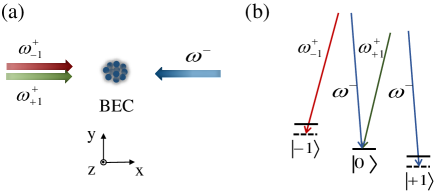
Figure 1: (a) Schematic of the system. A spin-1 BEC is illuminated by three Raman lasers so as to generate SO coupling. (b) The atomic level structure.

Incorporating the interatomic collisional interactions, the dynamics of the BEC are governed by the Gross-Pitaevskii (G-P) equation

$$i\hbar\frac{\partial\Psi}{\partial t}=\left(H_{S}+H_{I}\right)\Psi,$$ (3)

where $H_{I}$ is the mean-field Hamiltonian accounting for the nonlinear interaction between atoms,

$$H_{I}=\left(\begin{array}[]{ccc}\Gamma_{+1}&0&\Gamma_{-+}\\ 0&\Gamma_{0}&0\\ \Gamma_{-+}^{\ast}&0&\Gamma_{-1}\end{array}\right).$$ (4)

Here $\Gamma_{\pm 1}=(c_{0}+c_{2})\left|\psi_{\pm 1}\right|^{2}$, $\Gamma_{0}=(c_{0}+c_{2}/2)\left|\psi_{0}\right|^{2}$, and $\Gamma_{-+}=-2c_{2}\psi_{-1}^{\ast}\psi_{+1}$. The coefficients $c_{0}$ and $c_{2}$ describe density-density and spin-spin interaction strengths, respectively. Note that $c_{0,2}$ can be feasibly tuned through Feshbach resonances. In the following numerical calculations, we fix $c_{0}\sqrt{m/\hbar^{3}\omega}=0.05$ and take the typical ratio $c_{2}/c_{0}=-0.005$ for ⁸⁷Rb.

III Single particle spectrum

We first analyze the single-particle spectrum of the system. Notice that in the absence of the transverse potential ($\Omega=0$), the Hamiltonian (2) is exactly solvable, giving rise to the eigenstates

$$\left|\psi_{n,\chi}\right\rangle=\left|\psi_{n}^{\chi}\right\rangle\left|\chi\right\rangle,$$ (5)

where the spin part $\left|\chi\right\rangle$ is the eigenstate of the spin operator $F_{z}$, obeying $F_{z}\left|\chi\right\rangle=\chi\left|\chi\right\rangle$ with $\chi=0,\pm 1$, and the orbital part satisfies $\left|\psi_{n}^{\chi}\right\rangle\equiv\exp(-i\chi m\alpha x/\hbar)\left|\phi_{n}\right\rangle$. Here $\left|\phi_{n}\right\rangle$ is the $n$th eigenstate of a harmonic oscillator whose oscillation frequency is $\omega$. The eigenvalues of states (5) are given by

$$E_{n,\chi}=n\hbar\omega-\chi(\hbar\delta-\chi\hbar\epsilon).$$ (6)

It is thus clear that, due to the spin-1 nature of the BEC, the spectra are grouped as three different branches labeled by $\chi$, each of which contains a series of equally-distributed orbital levels. Moreover, without the linear and quadratic Zeeman fields, the orbital levels with the same quantum number $n$ appear to be triply degenerate with respect to the spin variation $\chi\longrightarrow\chi\pm 1$. A nonzero quadratic Zeeman field opens an energy splitting between $E_{n,0}$ and $E_{n,\pm 1}$ by $\hbar\epsilon$, and the degeneracy of the doublet $E_{n,+1}$ and $E_{n,-1}$ is lifted by the linear Zeeman field [see Fig. 2(a) for illustration]. It is to be noted that, by further increasing the quadratic and linear Zeeman fields, there exists a possibility that the eigenstates with different spin and orbital quantum numbers become degenerate again, namely $E_{n,\chi}=E_{n+k,\chi^{\prime}}$, where $k$ is a nonzero integer and $\chi\neq\chi^{\prime}$. This degeneracy may dramatically affect the dynamics of the BEC, as will be clarified in Sec. IV.

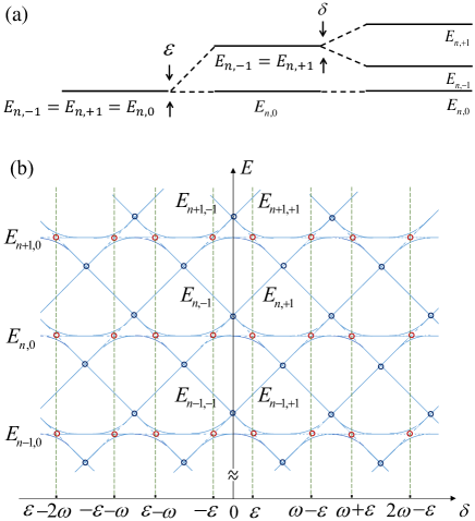
Figure 2: (a) Schematic energy levels of the $n$th orbit and their splitting under the action of the quadratic and linear Zeeman fields. (b) Schematic illustration of the single-particle spectrum (blue solid curve) as functions of the linear Zeeman field $\delta$ with certain fixed $\epsilon$. The red and blue circles indicate the level avoided crossing and level crossing points, respectively. The green dashed lines are intentionally added to pinpoint the resonant values of $\delta$.

Let us now turn on the transverse potential ($\Omega\neq 0$) and inspect its influences on the spectrum. Since the transverse term $\hbar\Omega F_{x}$ does not commute with the Hamiltonian, no exact solution exists. We work on the regime where $\Omega/\omega\ll 1$ so that the transverse potential can be treated perturbatively. Based on the standard perturbation theory, the eigenstates, which are accurate up to first order in $\Omega$, are summarized as

$$\left|\tilde{\psi}_{n,\chi}\right\rangle = \sum_{n^{\prime}=1}^{\infty}\left(C_{\chi,-1}^{n,n^{\prime}}\left|\psi_{n^{\prime}}^{-1}\right\rangle\left|-1\right\rangle+C_{\chi,0}^{n,n^{\prime}}\left|\psi_{n^{\prime}}^{0}\right\rangle\left|0\right\rangle\right.$$ (7)

$$\left.+C_{\chi,+1}^{n,n^{\prime}}\left|\psi_{n^{\prime}}^{+1}\right\rangle\left|+1\right\rangle\right),$$

where the detailed expressions of $C_{\chi,\chi^{\prime}}^{n,n^{\prime}}$ are given in the Appendix. It can be seen that the states $\left|\tilde{\psi}_{n,\chi}\right\rangle$ are no longer spin-orbit separable but in a form that spin and orbital parts are dressed together. Without the transverse potential ($\Omega=0$), we have $C_{\chi,\chi^{\prime}}^{n,n^{\prime}}=\delta_{\chi,\chi^{\prime}}\cdot\delta_{n,n^{\prime}}$ and the dressed state reduces to the bare one, $\left|\tilde{\psi}_{n,\chi}\right\rangle=\left|\psi_{n,\chi}\right\rangle$. Observing $\left\langle\psi_{n,\chi}\right|F_{x}\left|\psi_{n^{\prime},\chi^{\prime}}\right\rangle=\sqrt{2}(\delta_{n,n^{\prime}}\delta_{\chi,\chi^{\prime}+1}+\delta_{n,n^{\prime}}\delta_{\chi,\chi^{\prime}-1})/2$, the first order corrections of eigenvalues are generally zero so that corresponding eigenenergies remain the same as those without transverse potential, $\tilde{E}_{n,\chi}=E_{n,\chi}$. However, when energy levels differing by one unit of spin angular momentum get close to each other, saying $\left|E_{n,0}-E_{n+k,\pm 1}\right|\ll$ $\hbar\omega$, the coupling between them is intensively enhanced, leading to the break down of the non-degenerate perturbation formula. Employing a degenerate perturbation method, an avoided crossing between energy levels with $\left|\chi-\chi^{\prime}\right|=1$ appears, producing

$$\left\{\begin{array}[]{c}\tilde{E}_{n+k,0}=(n+k)\hbar\omega+\frac{\sqrt{2}}{2}\hbar\Omega\left|\eta\right|\\ \tilde{E}_{n,+1}=(n+k)\hbar\omega-\frac{\sqrt{2}}{2}\hbar\Omega\left|\eta\right|\\ \;\tilde{E}_{n,-1}=E_{n,-1}\end{array}\right.,$$ (8)

for $E_{n,+1}=E_{n+k,0}$, and

$$\left\{\begin{array}[]{c}\tilde{E}_{n,+1}=E_{n,+1}\\ \tilde{E}_{n+k,0}=(n+k)\hbar\omega+\frac{\sqrt{2}}{2}\hbar\Omega\left|\eta\right|\\ \tilde{E}_{n,-1}=(n+k)\hbar\omega-\frac{\sqrt{2}}{2}\hbar\Omega\left|\eta\right|\end{array}\right.,$$ (9)

for $E_{n,-1}=E_{n+k,0}$, with transverse-potential-induced splitting $\sqrt{2}\hbar\Omega\left|\eta\right|$ and $\eta=\left\langle\psi_{n}^{+1}\right|\left.\psi_{n+k}^{0}\right\rangle$ [see Fig. 2(b) for illustration]. Note that since $F_{x}$ does not couple states with spin angular momentum $+1$ and $-1$, the non-degenerate perturbation theory still applies for the case of $E_{n,+1}=E_{n+k,-1}$, at which a level crossing occurs instead.

IV Dynamical resonance

Armed with the knowledge of eigenstates and eigenenergies, we are in the right stage to study the collective dynamics. We first focus on the COM motion of the condensate subject to a sudden shift of the harmonic trapping potential. It is well known that for a regular BEC without SO coupling, the COM motion turns out to be a sinusoidal oscillation whose period depends only on the trapping frequency and is not affected by other parameters such as nonlinearity, shifting distance, and external Zeeman fields HCOM . The SO coupling, on the other hand, embeds the spin character of the BEC into its motional degrees of freedom ASOD2 ; ASOD3 ; ASOD4 . In view of this, the COM motion here is expected to respond to typical spin manipulations, which for instance, can be achieved by applying effective magnetic fields such as the linear and quadratic Zeeman fields.

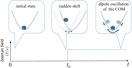
Figure 3: Schematic description of the proposed dynamical scheme for the Zeeman resonance. Top panel: Trapping potential and the corresponding COM motion of the BEC at different times. Bottom panel: Timing of the external Zeeman fields.

We assume the external Zeeman fields are switched off initially ($\delta=\epsilon=0$), and the BEC is prepared in a given state of the lowest orbital level, say $\left|\Psi(0)\right\rangle=\sum\nolimits_{\chi=-1}^{+1}C_{\chi}\left|\psi_{0}^{\chi}\right\rangle\left|\chi\right\rangle$, with $C_{\chi}$ being some superposition coefficient. The dynamics is activated at some time $t_{0}$ by a sudden shift of the trapping potential ASOD2 ; ASOD4 . Moreover, the trap shift is accompanied by an abruptly applied linear and quadratic Zeeman fields, as schematically illustrated in Fig. 3. Given this, the wavefunction for $t>t_{0}$ can be expanded in terms of the eigenstates $\left|\tilde{\psi}_{n,\chi}\right\rangle$ as

$$\left|\Psi(t)\right\rangle=\sum_{n=1}^{\infty}\sum_{\chi=-1}^{1}A_{n,\chi}e^{\frac{i}{\hbar}p_{x}D}\left|\tilde{\psi}_{n,\chi}\right\rangle e^{-\frac{i}{\hbar}\tilde{E}_{n,\chi}},$$ (10)

where $A_{n,\chi}=\left\langle\tilde{\psi}_{n,\chi}\right|\exp(-ip_{x}D/\hbar)\left|\Psi(0)\right\rangle$ with $D$ being the shifting distance. With this wave function, the time evolution of the COM is expressed as

$$\left\langle x(t)\right\rangle \!\!\!=\!\!\! \sum_{n=1}^{\infty}\sum_{n^{\prime}=1}^{\infty}\sum_{\chi=-1}^{1}\sum_{\chi^{\prime}=-1}^{1}\sqrt{\frac{m\omega}{\hbar}}R_{\chi,\chi^{\prime}}^{n,n^{\prime}}e^{-\frac{i}{\hbar}\left(\tilde{E}_{n,\chi}-\tilde{E}_{n^{\prime},\chi^{\prime}}\right)t}$$ (11)

$$+D,$$

where $\left\langle\cdot\cdot\cdot\right\rangle$ stands for the spacial average over condensate wave function, and we have introduced the dimensionless term $R_{\chi,\chi^{\prime}}^{n,n^{\prime}}=\sqrt{\hbar/m\omega}A_{n^{\prime},\chi^{\prime}}^{\ast}A_{n,\chi}\left\langle\tilde{\psi}_{n^{\prime},\chi^{\prime}}\right|x\left|\tilde{\psi}_{n,\chi}\right\rangle$. Note that in Eq. (11), while terms multiplied by the dynamical phase factors, $\exp[-i(\tilde{E}_{n,\chi}-\tilde{E}_{n^{\prime},\chi^{\prime}})t/\hbar]$, are responsible for the time-dependent oscillation, the shifting distance $D$ appearing in the last term represents a constant equilibrium position around which the BEC oscillates. As we are only interested in the dynamical part of the oscillation, it is more convenient to focus on the redefined COM motion in which the constant shifting distance is deducted, i.e., $\left\langle\overline{x(t)}\right\rangle=\left\langle x(t)\right\rangle-D$. Inspired by the fact that quantum particles in a given state are essentially nonlocal in their spacial dimensions, it is expected that there may be some physical information nonlocally hidden in the time dimension of wave functions. This motivate us to investigate the time-averaged quantity

$$Q(\mathcal{O})=\frac{1}{T}\left|\int_{t_{0}}^{t_{0}+T}\left\langle\mathcal{O}\right\rangle dt\right|,$$ (12)

where $T$ is a long-time span and $\mathcal{O}$ is the physical observable over which the average is taken ASOD5 . Equation (12) can be treated as a kind of coarse-grained averaging, as the dynamical details at any specific time become irrelevant. Nevertheless, potential dynamical effects accumulated through a long-time evolution are remarkably highlighted under this framework.

As depicted in Fig. 4(a), the long-time-averaged COM motion, $Q[\overline{x(t)}]$, as a function of $\delta$ for various $\epsilon$ with the initial state $\left|\Psi(0)\right\rangle=(\left|\psi_{0}^{-1}\right\rangle\left|-1\right\rangle+\left|\psi_{0}^{0}\right\rangle\left|0\right\rangle+\left|\psi_{0}^{+1}\right\rangle\left|+1\right\rangle)/\sqrt{3}$, is obtained by numerically solving the G-P equation (3). An intriguing finding is that a series of resonant peaks are formed at some specific linear Zeeman fields, whose values appear to be affected by the strength of the quadratic Zeeman field. That is, for $\epsilon/\omega=1$, the resonance occurs at integer values of $\delta/\omega$, whereas for $\epsilon/\omega=0.5$, the resonant points of $\delta/\omega$ become half-integer. This phenomena can be viewed as a consequence of the out-of-phase interference among different spin-orbit states.

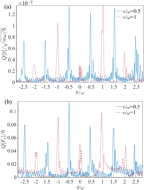
Figure 4: The long-time-averaged quantity (a) $Q[\overline{x(t)}]$ and (b) $Q[F_{x}(t)]$ as functions of the linear Zeeman field $\delta$ for $\epsilon/\omega=0.5$ (blue-solid curve) and $\epsilon/\omega=1$ (red-dashed curve), with the initial state $\left|\Psi(0)\right\rangle=(\left|\psi_{0}^{-1}\right\rangle\left|-1\right\rangle+\left|\psi_{0}^{0}\right\rangle\left|0\right\rangle+\left|\psi_{0}^{+1}\right\rangle\left|+1\right\rangle)/\sqrt{3}$. The other parameters are $T=70/\omega$, $D/\sqrt{m\omega/\hbar}=2$, $\Omega/\omega=0.05$ and $\alpha=2$.

To understand this clearly, attention should be turned to the dynamical phase factors $\exp[-i(\tilde{E}_{n,\chi}-\tilde{E}_{n^{\prime},\chi^{\prime}})t/\hbar]$ and the corresponding terms $R_{\chi,\chi^{\prime}}^{n,n^{\prime}}$ in Eq. (11). Note that the dynamical phases in the form of $(\tilde{E}_{n,\chi}-\tilde{E}_{n^{\prime},\chi^{\prime}})t/\hbar$ with $\chi\neq\chi^{\prime}$ strongly depend on both the two Zeeman fields $\delta$ and $\epsilon$, whereas those possessing a single spin subscript $\chi$, namely $-i(\tilde{E}_{n,\chi}-\tilde{E}_{n^{\prime},\chi})t/\hbar$, do not. It is thus expected that the former should play the key role in any Zeeman-field-related responses. In fact, for general values of $\delta$ and $\epsilon$, the diagonal terms $R_{\chi,\chi}^{n,n}$ are negligibly small since they are shown to be proportional to $(\Omega/\omega)^{2}$ (See Appendix for details), and it is the energy differences, $\tilde{E}_{n,\chi}-\tilde{E}_{n^{\prime},\chi^{\prime}}$ ($n\neq n^{\prime}$ and $\chi\neq\chi^{\prime}$), which are on the order of a few $\hbar\omega$, that dominates the time evolution of the BEC. As a result, the dynamical parts in Eq. (11) oscillate fast over time, making $Q[\overline{x(t)}]$ tend to vanish due to the out-of-phase interference. However, tuning Zeeman fields to the level avoided crossing point with $E_{n,0}=E_{n+k,\pm 1}$, we get a maximally minimized energy difference, satisfying $\left|\tilde{E}_{n,\chi}-\tilde{E}_{n^{\prime},\chi^{\prime}}\right|/\hbar\omega=\sqrt{2}\left|\eta\right|\Omega/\omega\ll 1$, which dramatically slows down the time oscillation of the phase factors. Hence, the out-of-phase interference is suppressed to the largest extent, giving rise to a considerable non-zero contribution to $Q[\overline{x(t)}]$. It follows that the level avoided crossing point, at which the Zeeman fields $\delta$ and $\epsilon$ satisfy

$$\delta\pm\epsilon=k\omega,$$ (13)

is nothing but the point at which the dynamical resonance occurs. The resonant condition Eq. (13) is the main result of this paper.

Along this reasoning, it seems that there should exist similar resonant peaks at the level crossing point with $E_{n,+1}=E_{n+k,-1}$ as well [See, for example, the blue circles in Fig. 2(b)]. However, a straightforward calculation shows that, at this point, $R_{+1,-1}^{n,n+k}$ is on the order of $(\Omega/\omega)^{2}A_{n^{\prime},\chi^{\prime}}^{\ast}A_{n,\chi}$, which turns out to be vanishingly small in the perturbation regime. Thus, the suppression of out-of-phase interference can generate little contribution to $Q[\overline{x(t)}]$, resulting in the absence of the expected dynamical resonance. Figure 5 plots the coordinates of resonant peaks in the $\epsilon-$ $\delta$ plane, which is obtained by numerically solving the G-P equation (3). It is shown that the numerical results are in quantitative agreement with Eq. (13). The resonance condition in Eq. (13) is simple and quite generic in the sense that it bridges between the linear and quadratic Zeeman fields via only the trapping frequency $\omega$, and is independent of other parameters such as the shifting distance $D$, the time span $T$, and the SO coupling strength $\alpha$. This property offers interesting opportunities for the Zeeman-fields-based quantum metrology.

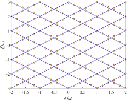
Figure 5: Plot of resonance condition in the $\epsilon-\delta$ plane. The blue solid curves correspond to the analytical relation in Eq. (13). The red circles (yellow diamonds) come from numerical results of $Q[\overline{x(t)}]$ ($Q[F_{x}(t)]$) obtained by solving the G-P equation (3). The initial state and other parameters used in the numerical calculations are the same as those in Fig. 4.

Instead of responding linearly to the Zeeman fields, as is known for systems without SO coupling, the spin polarization here may exhibit similar resonant behavior. The physics follows that of the COM motion. Invoking the wave function in Eq. (10), the $i$th component ($i=x,y,z$) of the spin polarization is written as

$$\left\langle F_{i}(t)\right\rangle=\sum_{n=1}^{\infty}\sum_{n^{\prime}=1}^{\infty}\sum_{\chi=-1}^{1}\sum_{\chi^{\prime}=-1}^{1}\hbar R_{\chi,\chi^{\prime}}^{(i),n,n^{\prime}}e^{-\frac{i}{\hbar}\left(\tilde{E}_{n,\chi}-\tilde{E}_{n^{\prime},\chi^{\prime}}\right)t},$$ (14)

with $R_{\chi,\chi^{\prime}}^{(i),n,n^{\prime}}=A_{n^{\prime},\chi^{\prime}}^{\ast}A_{n,\chi}\left\langle\tilde{\psi}_{n^{\prime},\chi^{\prime}}\right|F_{i}\left|\tilde{\psi}_{n,\chi}\right\rangle/\hbar$. As described above, one of the key points of the Zeeman resonance lies in the fact that the off-diagonal terms $R_{\chi,\chi^{\prime}}^{(i),n,n^{\prime}}$ dominate over the diagonal ones $R_{\chi,\chi}^{(i),n,n\text{ }}$outside the level avoided crossing points. This motivates us to focus on the spin polarization along the transverse directions (i.e., directions in the $x-y$ plane), since in this case $R_{\chi,\chi}^{(i),n,n}$ is negligible compared to $R_{\chi,\chi^{\prime}}^{(i),n,n^{\prime}}$ in the sense that $R_{\chi,\chi}^{(i),n,n}/R_{\chi,\chi^{\prime}}^{(i),n,n^{\prime}}\sim\Omega/\omega$. Following the same derivation as that used in analyzing the COM motion, we can reproduce the resonance condition in Eq. (13) straightforwardly. Figure 4(b) shows the numerical results of $Q[F_{x}(t)]$ as a function of $\delta$ for various $\epsilon$, whose peak positions are well described by Eq. (13). More numerical results of peak positions in the $\epsilon-$ $\delta$ plane are shown in Fig. 5, which agree with Eq. (13) as expected.

It is worth noting that, our discussion about the proposed Zeeman resonance is not affected by different choices of the initial state $\left|\Psi(0)\right\rangle$, provided that it is a superposition of the three Zeeman sublevels $\left|+1\right\rangle$, $\left|0\right\rangle$, and $\left|-1\right\rangle$. Easy to be satisfied in the current experiment with cold atoms, this constraint on $\left|\Psi(0)\right\rangle$ guarantees the off-diagonal terms $R_{\chi,\chi^{\prime}}^{n,n^{\prime}}$ and $R_{\chi,\chi^{\prime}}^{(x),n,n^{\prime}}$ nonzero, which is necessary to support visible resonant peaks.

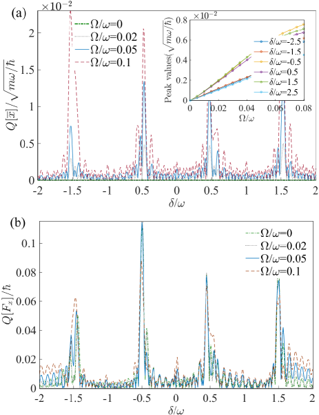
Figure 6: The long-time-averaged quantity, $Q[\overline{x(t)}]$ (a) and $Q[F_{x}(t)]$ (b), as functions of the linear Zeeman field $\delta$ for $\epsilon/\omega=0.5$ (blue-solid curve) and different transverse potentials $\Omega$. Inset: The peak values of $Q[\overline{x(t)}]$ as a function of $\Omega/\omega$. The initial state and the other parameters are the same as those in Fig. 4.

We emphasize that the although the transverse potential $\Omega$ is not explicitly involved in Eq. (13), it plays a significant role in inducing the dynamical Zeeman resonance of the COM motion. It is easy to check that, in the absence of $\Omega$, the off-diagonal terms, $R_{\chi,\chi^{\prime}}^{n,n^{\prime}}$ with $\chi\neq\chi^{\prime}$, vanish, owing to the orthogonality between different spin states. This further erases the corresponding phase factors, $\exp[-i(\tilde{E}_{n,\chi}-\tilde{E}_{n^{\prime},\chi^{\prime}})t/\hbar]$, in Eq. (11) so that the dynamical resonant effect disappears. A nonzero transverse potential, on the other hand, dresses orbital states in different spin branches, as described by Eq. (7). This renders $R_{\chi,\chi^{\prime}}^{n,n^{\prime}}$ acquire finite values and thus validates the resonance condition in Eq. (13). In Fig. 6(a), we plot $Q[\overline{x(t)}]$ versus $\delta$ for different $\Omega$ with $\epsilon/\omega=0.5$. This figure shows that, each peak of $Q[\overline{x(t)}]$ increases in height as $\Omega$ increases. Especially for $\Omega=0$, no peaks can be found. Indeed, around the level avoided crossing point, the leading order of terms $R_{\chi,\chi^{\prime}}^{n,n^{\prime}}$ are shown to be $\Omega/\omega$. This signals that the peak values of $Q[\overline{x(t)}]$ may scale as $\Omega$ when the transverse potential is weak enough. In the inset of Fig. 6(a), we numerically plot various peak values of $Q[\overline{x(t)}]$ as functions of $\Omega/\omega$. It is found that these peak values can be well described by linear functions of $\Omega$ for $\Omega/\omega\lesssim 0.03$. Interestingly, in contract to the COM motion, the resonant peaks of spin polarizations appear to have no explicit dependence on $\Omega$, and they persist even for $\Omega=0$ [see Fig. 6(b)]. This is because $F_{x}$ couple states with different spin angular momentum, yielding $R_{\chi,\chi^{\prime}}^{(x),n,n^{\prime}}\neq 0$, regardless of the explicit value of $\Omega$.

V Conclusions

In conclusion, we have investigated the orbital and spin dynamics of a SO-coupled spin-1 BEC, and unraveled a Zeeman-field-induced resonant effect in this system. The resonant signature is encoded in the time-averaged COM oscillation and spin polarizations, which exhibit remarkable peaks when the Zeeman fields are tuned to certain strengths. The underlying physics behind this resonance can be attributed to the out-of-phase interference of the dynamical phases carried by different SO states. We have also derived an analytical expression for the resonant condition. This expression set a connection between the linear and quadratic Zeeman fields, and may thus facilitate applications in quantum information and quantum precision measurement.

Appendix A perturbation calculations

In this Appendix, we provide the detailed derivation of the eigenstates in Eq. (7) and eigenenergies Eqs. (8) and (9) of the main text, based on the perturbation theory. For general parameters, the unperturbed eigenenergies are non-degenerate and thus the non-degenerate perturbation formula applies. The eigenstates, which are accurate up to first order in $\hbar\Omega$, are obtained as

$$\left|\tilde{\psi}_{n,\pm 1}\right\rangle = \left|\psi_{n}^{\pm 1}\right\rangle\left|\pm 1\right\rangle$$

$$+\frac{\sqrt{2}\hbar\Omega}{2}\sum_{n^{\prime}=1}^{\infty}\frac{\left\langle\psi_{n^{\prime}}^{0}\right.\left|\psi_{n}^{\pm 1}\right\rangle}{(n-n^{\prime})\hbar\omega\mp\hbar\delta+\hbar\varepsilon}\left|\psi_{n^{\prime}}^{0}\right\rangle\left|0\right\rangle,$$

$$\left|\tilde{\psi}_{n,0}\right\rangle = \left|\psi_{n}^{0}\right\rangle\left|0\right\rangle$$

$$+\frac{\sqrt{2}\hbar\Omega}{2}\sum_{n^{\prime}=1}^{\infty}\frac{\left\langle\psi_{n^{\prime}}^{+1}\right.\left|\psi_{n}^{0}\right\rangle}{(n-n^{\prime})\hbar\omega+\hbar\delta-\hbar\varepsilon}\left|\psi_{n^{\prime}}^{+1}\right\rangle\left|+1\right\rangle$$

$$+\frac{\sqrt{2}\hbar\Omega}{2}\sum_{n^{\prime}=1}^{\infty}\frac{\left\langle\psi_{n^{\prime}}^{-1}\right.\left|\psi_{n}^{0}\right\rangle}{(n-n^{\prime})\hbar\omega-\hbar\delta-\hbar\varepsilon}\left|\psi_{n^{\prime}}^{-1}\right\rangle\left|-1\right\rangle.$$

The corresponding eigenenergies are $\tilde{E}_{n,\chi}=E_{n,\chi}+\hbar\Omega\left\langle\psi_{n,\chi}\right|F_{x}\left|\psi_{n,\chi}\right\rangle=E_{n,\chi}$. With the states in Eqs. (A) and (A), we can readily make the following estimation of orders: $R_{\chi,\chi}^{n,n}/(A_{n^{\prime},\chi^{\prime}}^{\ast}A_{n,\chi})\sim(\Omega/\omega)^{2}$, $R_{0,\pm 1}^{n,n^{\prime}}/(A_{n^{\prime},\chi^{\prime}}^{\ast}A_{n,\chi})\sim\Omega/\omega$, $R_{\chi,\chi}^{(x/y),n,n}/(A_{n^{\prime},\chi^{\prime}}^{\ast}A_{n,\chi})\sim\Omega/\omega$, and $R_{0,\pm 1}^{(x/y),n,n^{\prime}}/(A_{n^{\prime},\chi^{\prime}}^{\ast}A_{n,\chi})\sim 1$.

However, when the energy levels are tuned to the level avoided crossing point where $\left|E_{n,\chi}-E_{n+k,\chi^{\prime}}\right|\ll$ $\hbar\omega$, we should employ the degenerate perturbation theory. Assuming, for instance, $E_{n,+1}=E_{n+k,0}$, the degenerate subspace is spanned by $\left|\psi_{n,+1}\right\rangle$ and $\left|\psi_{n+k,0}\right\rangle$. The secular equation of the perturbation matrix in this subspace, det$\left|\hbar\Omega\left\langle\psi_{n,\chi}\right|F_{x}\left|\psi_{n+k,\chi^{\prime}}\right\rangle-E^{(1)}\delta_{\chi\chi^{\prime}}\right|=0$, is expressed explicitly as

$$\left|\begin{array}[]{cc}-E^{(1)}&\frac{\sqrt{2}\hbar\Omega}{2}\eta\\ \frac{\sqrt{2}\hbar\Omega}{2}\eta^{\ast}&-E^{(1)}\end{array}\right|=0,$$ (17)

where $\eta=\left\langle\psi_{n}^{+1}\right.\left|\psi_{n+k}^{0}\right\rangle$. Note that since $\eta$ is generally small, we have neglected its dependence on $n$ and $k$ for simplicity. It follows that the first-order corrections of the eigenenergies are $E_{\pm}^{(1)}=\pm\sqrt{2}\hbar\Omega\left|\eta\right|/2$, giving rise to

$$\left\{\begin{array}[]{c}\tilde{E}_{n+k,0}=E_{n,0}+E_{+}^{(1)}=(n+k)\hbar\omega+\frac{\sqrt{2}}{2}\hbar\Omega\left|\eta\right|\\ \tilde{E}_{n,+1}=E_{n,+1}+E_{-}^{(1)}=(n+k)\hbar\omega-\frac{\sqrt{2}}{2}\hbar\Omega\left|\eta\right|\\ \tilde{E}_{n,-1}=E_{n,-1}\end{array}\right.,$$ (18)

and the proper zeroth-order eigenstates are

$$\left\{\begin{array}[]{c}\left|\psi_{n,+1}^{(0)}\right\rangle=\frac{\sqrt{2}}{2}(\frac{\eta}{\left|\eta\right|}\left|\psi_{n,1}\right\rangle+\left|\psi_{n+k,0}\right\rangle)\\ \left|\psi_{n,0}^{(0)}\right\rangle=\frac{\sqrt{2}}{2}(-\frac{\eta}{\left|\eta\right|}\left|\psi_{n,1}\right\rangle+\left|\psi_{n+k,0}\right\rangle)\\ \left|\psi_{n,-1}^{(0)}\right\rangle=\left|\psi_{n,-1}\right\rangle\end{array}\right..$$ (19)

With the states in Eq. (19), it is straightforward to derive the first-order perturbative eigenstates using the non-perturbation theory. The resulting eigenstate takes the form of Eq. (7), i.e.,

$$\left|\tilde{\psi}_{n,\chi}\right\rangle = \sum_{n^{\prime}=1}^{\infty}\left(C_{\chi,-1}^{n,n^{\prime}}\left|\psi_{n^{\prime}}^{-1}\right\rangle\left|-1\right\rangle+C_{\chi,0}^{n,n^{\prime}}\left|\psi_{n^{\prime}}^{0}\right\rangle\left|0\right\rangle\right.$$ (20)

$$\left.+C_{\chi,+1}^{n,n^{\prime}}\left|\psi_{n^{\prime}}^{+1}\right\rangle\left|+1\right\rangle\right),$$

where

$$C_{+1,+1}^{n,n^{\prime}} = \frac{\sqrt{2}}{2}\frac{\eta}{\left|\eta\right|}+\frac{\hbar\Omega}{2}\frac{\left\langle\psi_{n^{\prime}}^{+1}\right.\left|\psi_{n+k}^{0}\right\rangle}{(n-n^{\prime}+k)\hbar\omega+\sqrt{2}\hbar\Omega/2+\hbar\delta-\hbar\varepsilon},$$

$$C_{+1,0}^{n,n^{\prime}} = \frac{\sqrt{2}}{2}+\frac{\hbar\Omega}{2}\frac{\eta}{\left|\eta\right|}(1+\frac{\sqrt{2}}{2}\delta_{n^{\prime},n+k})\frac{\left\langle\psi_{n^{\prime}}^{0}\right.\left|\psi_{n}^{1}\right\rangle}{(n-n^{\prime}+k)\hbar\omega+\sqrt{2}\hbar\Omega/2},$$

$$C_{+1,-1}^{n,n^{\prime}} = \frac{\hbar\Omega}{2}\frac{\left\langle\psi_{n^{\prime}}^{-1}\right.\left|\psi_{n+1}^{0}\right\rangle}{(n-n^{\prime}+k)\hbar\omega+\sqrt{2}\hbar\Omega/2-\hbar\delta-\hbar\varepsilon},$$

$$C_{0,+1}^{n,n^{\prime}} = -\frac{\sqrt{2}}{2}\frac{\eta}{\left|\eta\right|}+\frac{\hbar\Omega}{2}\frac{\left\langle\psi_{n^{\prime}}^{+1}\right.\left|\psi_{n+k}^{0}\right\rangle}{(n-n^{\prime}+k)\hbar\omega-\sqrt{2}\hbar\Omega/2+\hbar\delta-\hbar\varepsilon},$$

$$C_{0,0}^{n,n^{\prime}} = \frac{\sqrt{2}}{2}-\frac{\hbar\Omega}{2}\frac{\eta}{\left|\eta\right|}(1+\frac{\sqrt{2}}{2}\delta_{n^{\prime},n+k})\frac{\left\langle\psi_{n^{\prime}}^{0}\right.\left|\psi_{n}^{1}\right\rangle}{(n-n^{\prime}+k)\hbar\omega-\sqrt{2}\hbar\Omega/2},$$

$$C_{0,-1}^{n,n^{\prime}} = \frac{\hbar\Omega}{2}\frac{\left\langle\psi_{n^{\prime}}^{-1}\right.\left|\psi_{n+1}^{0}\right\rangle}{(n-n^{\prime}+k)\hbar\omega-\sqrt{2}\hbar\Omega/2-\hbar\delta-\hbar\varepsilon},$$

$$C_{-1,+1}^{n,n^{\prime}} = 0,\ C_{-1,-1}^{n,n^{\prime}}=1,$$

$$C_{-1,0}^{n,n^{\prime}} = \frac{\sqrt{2}\hbar\Omega}{2}\frac{\left\langle\psi_{n^{\prime}}^{0}\right.\left|\psi_{n}^{-1}\right\rangle}{(n-n^{\prime})\hbar\omega+\hbar\delta+\hbar\varepsilon}.$$

Following exactly the same procedure, we can readily obtain the eigenenergies and eigenstates for the case of $E_{n,-1}=E_{n+k,0}$. Accurate up to first order in $\Omega$, the eigenenergies are given by

$$\left\{\begin{array}[]{c}\tilde{E}_{n,+1}=E_{n,+1}\\ \tilde{E}_{n+k,0}=(n+k)\hbar\omega+\frac{\sqrt{2}}{2}\hbar\Omega\left|\eta\right|\\ \tilde{E}_{n,-1}=(n+k)\hbar\omega-\frac{\sqrt{2}}{2}\hbar\Omega\left|\eta\right|\end{array}\right.,$$ (21)

and the coefficients $C_{\chi,\chi^{\prime}}^{n,n^{\prime}}$ in the eigenstate $\left|\tilde{\psi}_{n,\chi}\right\rangle$ become

$$C_{+1,+1}^{n,n^{\prime}} = 1,\ C_{+1,-1}^{n,n^{\prime}}=0,$$

$$C_{+1,0}^{n,n^{\prime}} = \frac{\sqrt{2}\hbar\Omega}{2}\frac{\left\langle\psi_{n^{\prime}}^{0}\right.\left|\psi_{n}^{+1}\right\rangle}{(n-n^{\prime})\hbar\omega-\hbar\delta+\hbar\varepsilon},$$

$$C_{0,+1}^{n,n^{\prime}} = \frac{\hbar\Omega}{2}\frac{\left\langle\psi_{n^{\prime}}^{+1}\right.\left|\psi_{n+k}^{0}\right\rangle}{(n-n^{\prime}+k)\hbar\omega+\sqrt{2}\hbar\Omega/2+\hbar\delta-\hbar\varepsilon},$$

$$C_{0,0}^{n,n^{\prime}} = \frac{\sqrt{2}}{2}+\frac{\hbar\Omega}{2}\frac{\eta}{\left|\eta\right|}(1+\frac{\sqrt{2}}{2}\delta_{n^{\prime},n+k})\frac{\left\langle\psi_{n^{\prime}}^{0}\right.\left|\psi_{n}^{-1}\right\rangle}{(n-n^{\prime}+k)\hbar\omega+\sqrt{2}\hbar\Omega/2},$$

$$C_{0,-1}^{n,n^{\prime}} = \frac{\hbar\Omega}{2}\frac{\left\langle\psi_{n^{\prime}}^{-1}\right.\left|\psi_{n+1}^{0}\right\rangle}{(n-n^{\prime}+k)\hbar\omega+\sqrt{2}\hbar\Omega/2-\hbar\delta-\hbar\varepsilon},$$

$$C_{-1,+1}^{n,n^{\prime}} = \frac{\hbar\Omega}{2}\frac{\left\langle\psi_{n^{\prime}}^{+1}\right.\left|\psi_{n+k}^{0}\right\rangle}{(n-n^{\prime}+k)\hbar\omega-\sqrt{2}\hbar\Omega/2+\hbar\delta-\hbar\varepsilon},$$

$$C_{-1,0}^{n,n^{\prime}} = \frac{\sqrt{2}}{2}+\frac{\hbar\Omega}{2}\frac{\eta}{\left|\eta\right|}(1+\frac{\sqrt{2}}{2}\delta_{n^{\prime},n+k})\frac{\left\langle\psi_{n^{\prime}}^{0}\right.\left|\psi_{n}^{-1}\right\rangle}{(n-n^{\prime}+k)\hbar\omega-\sqrt{2}\hbar\Omega/2},$$

$$C_{-1,-1}^{n,n^{\prime}} = \frac{\sqrt{2}}{2}\frac{\eta}{\left|\eta\right|}+\frac{\hbar\Omega}{2}\frac{\left\langle\psi_{n^{\prime}}^{-1}\right.\left|\psi_{n+1}^{0}\right\rangle}{(n-n^{\prime}+k)\hbar\omega-\sqrt{2}\hbar\Omega/2-\hbar\delta-\hbar\varepsilon}.$$

References

• (1) D. J. E. Callaway and A. Rahman, Microcanonlcal Ensemble Formulation of Lattice Gauge Theory, Phys. Rev. Lett. 49, 613 (1982).
• (2) G. Vignale and M. Rasolt, Current- and spin-density-functional theory for inhomogeneous electronic systems in strong magnetic fields, Phys. Rev. B 37, 10685 (1988).
• (3) D. Xiao, M.-C. Chang, and Q. Niu, Berry phase effects on electronic properties, Rev. Mod. Phys. 82, 1959 (2010).
• (4) M. Hasan and C. Kane, Colloquium: Topological insulators, Rev. Mod. Phys. 82. 3045 (2010).
• (5) X.-L. Qi and S.-C. Zhang, Topological insulators and superconductors, Rev. Mod. Phys. 83, 1057 (2011).
• (6) I. B. Spielman, Raman processes and effective gauge potentials, Phys. Rev. A 79, 063613 (2009).
• (7) J. Dalibard, F. Gerbier, G. Juzeliūnas, and P. Őhberg, Colloquium: Artificial gauge potentials for neutral atoms, Rev. Mod. Phys. 83, 1523 (2011).
• (8) P.Wang, Z.-Q. Yu, Z. Fu, J. Miao, L. Huang, S. Chai, H. Zhai, and J. Zhang, Spin-Orbit Coupled Degenerate Fermi Gases, Phys. Rev. Lett. 109, 095301 (2012).
• (9) L. W. Cheuk, A. T. Sommer, Z. Hadzibabic, T. Yefsah, W. S. Bakr, and M. W. Zwierlein, Spin-Injection Spectroscopy of a Spin-Orbit Coupled Fermi Gas, Phys. Rev. Lett. 109, 095302 (2012).
• (10) Y.-J. Lin, K. Jiménez-García, and I. B. Spielman, Spin-orbit coupled Bose-Einstein condensates, Nature (London) 471, 83 (2011).
• (11) T. D. Stanescu, B. Anderson, and V. Galitski, Spin-orbit coupled Bose-Einstein condensates, Phys. Rev. A 78, 023616 (2008).
• (12) C. Wang, C. Gao, C.-M. Jian, and H. Zhai, Spin-Orbit Coupled Spinor Bose-Einstein Condensates, Phys. Rev. Lett. 105, 160403 (2010).
• (13) C. Wu, I. Mondragon-Shem, and X.-F. Zhou, Unconventional Bose-Einstein condensations from spin-orbit coupling, Chin. Phys. Lett. 28, 097102 (2011).
• (14) T.-L. Ho and S. Zhang, Bose-Einstein Condensates with Spin Orbit Interaction, Phys. Rev. Lett. 107, 150403 (2011).
• (15) M. Gong, S. Tewari, and C. Zhang, BCS-BEC Crossover and Topological Phase Transition in 3D Spin-Orbit Coupled Degenerate Fermi Gases, Phys. Rev. Lett. 107, 195303 (2011).
• (16) H. Hu, L. Jiang, X.-J. Liu, and H. Pu, Probing Anisotropic Superfluidity in Atomic Fermi Gases with Rashba Spin-Orbit Coupling, Phys. Rev. Lett. 107, 195304 (2011).
• (17) Z.-Q. Yu and H. Zhai, Spin-orbit Coupled Fermi Gases Across a Feshbach Resonance, Phys. Rev. Lett. 107, 195305 (2011).
• (18) H. Hu, B. Ramachandhran, H. Pu, and X.-J. Liu, Spin-Orbit Coupled Weakly Interacting Bose-Einstein Condensates in Harmonic Traps, Phys. Rev. Lett. 108, 010402 (2012).
• (19) T. Ozawa and G. Baym, Stability of Ultracold Atomic Bose Condensates with Rashba Spin-Orbit Coupling Against Quantum and Thermal Fluctuations, Phys. Rev. Lett. 109, 025301 (2012).
• (20) Y. Li, L. P. Pitaevskii, and S. Stringari, Quantum Tricriticality and Phase Transitions in Spin-Orbit Coupled Bose-Einstein Condensates, Phys. Rev. Lett. 108, 225301 (2012).
• (21) H. Zhai, Degenerate quantum gases with spin-orbit coupling, Rep. Prog. Phys. 78, 026001 (2015).
• (22) J.-R. Li, J. Lee, W. Huang, S. Burchesky, B. Shteynas, F. C. Top, A. O. Jamison, and W. Ketterle, A stripe phase with supersolid properties in spin-orbit-coupled Bose-Einstein con densates, Nature (London) 543, 91 (2017).
• (23) R. Liao, Searching for Supersolidity in Ultracold Atomic Bose Condensates with Rashba Spin-Orbit Coupling, Phys. Rev. Lett. 120, 140403 (2018).
• (24) W. Han, X.-F. Zhang, D.-S. Wang, H.-F. Jiang, W. Zhang, and S.-G. Zhang, Chiral Supersolid in Spin-Orbit-Coupled Bose Gases with Soft-Core Long-Range Interactions, Phys. Rev. Lett. 121, 030404 (2018).
• (25) J.-Y. Zhang, S.-C. Ji, Z. Chen, L. Zhang, Z.-D. Du, B. Yan, G.-S. Pan, B. Zhao, Y.-J. Deng, H. Zhai, S. Chen, and J.-W. Pan, Collective Dipole Oscillations of a Spin-Orbit Coupled Bose-Einstein Condensate, Phys. Rev. Lett. 109, 115301 (2012).
• (26) Y. Zhang, L. Mao, and C. Zhang, Mean-Field Dynamics of Spin Orbit Coupled Bose-Einstein Condensates, Phys. Rev. Lett. 108, 035302 (2012).
• (27) C. Qu, C. Hamner, M. Gong, C. Zhang, and P. Engels, Observation of Zitterbewegung in a spin-orbit-coupled Bose Einstein condensate, Phys. Rev. A 88, 021604(R) (2013).
• (28) Y. Zhang, G. Chen, and C. Zhang, Tunable Spin-orbit Coupling and Quantum Phase Transition in a Trapped Bose-Einstein Condensate, Sci. Rep. 3, 1937 (2013).
• (29) C. Wu, J. Fan, G. Chen, and S. Jia, Spin dynamics of a spin-orbit-coupled Bose-Einstein condensate in a shaken harmonic trap, Phys. Rev. A 99, 013617 (2019).
• (30) Y. Zhang, Z. Gui, and Y. Chen, Nonlinear dynamics of a spin-orbit-coupled Bose-Einstein condensate, Phys. Rev. A 99, 023616 (2019).
• (31) T.-L. Ho, Spinor Bose Condensates in Optical Traps, Phys. Rev. Lett. 81, 742 (1998).
• (32) T. Ohmi and K. Machida, Bose-Einstein condensation with internal degrees of freedom in alkali atom gases, J. Phys. Soc. Jpn. 67, 1822 (1998).
• (33) D. M. Stamper-Kurn and M. Ueda, Spinor Bose gases: Symme tries, magnetism, and quantum dynamics, Rev. Mod. Phys. 85, 1191 (2013).
• (34) Y. Huang, Y. Zhang, R. Lu, X. Wang, and S. Y, Macroscopic quantum coherence in spinor condensates confined in an anisotropic potential, Phys. Rev. A 86, 043625 (2012).
• (35) H. Xing, A. Wang, Q.-S. Tan, W. Zhang, and S. Y, Heisenberg-scaled magnetometer with dipolar spin-1 condensates, Phys. Rev. A 93, 043615 (2016).
• (36) Z. Pu, J. Zhang, S. Yi, D. Wang, and W. Zhang, Magnetic-field-induced dynamical instabilities in an antiferromagnetic spin-1 Bose-Einstein condensate, Phys. Rev. A 93, 053628 (2016).
• (37) S.-X. Deng, T. Shi, and S. Yi, Spin excitations in dipolar spin-1 condensates, Phys. Rev. A 102, 013305 (2020).
• (38) Z. Lan and P. Öhberg, Raman-dressed spin-1 spin-orbit-coupled quantum gas, Phys. Rev. A 89, 023630 (2014).
• (39) S. S. Natu, X. Li, and W. S. Cole, Striped ferronematic ground states in a spin-orbit-coupled S=1 Bose gas, Phys. Rev. A 91, 023608 (2015).
• (40) K. Sun, C. Qu, Y. Xu, Y. Zhang, and C. Zhang, Interacting spin-orbit-coupled spin-1 Bose-Einstein condensates, Phys. Rev. A 93, 023615 (2016).
• (41) G. I. Martone, F. V. Pepe, P. Facchi, S. Pascazio, and S. Stringari, Tricriticalities and Quantum Phases in Spin-Orbit-Coupled Spin-1 Bose Gases, Phys. Rev. Lett. 117, 125301 (2016).
• (42) Z.-Q. Yu, Phase transitions and elementary excitations in spin-1 Bose gases with Raman-induced spin-orbit coupling, Phys. Rev. A 93, 033648 (2016).
• (43) X.-W. Luo, K. Sun, and C. Zhang, Spin-Tensor-Momentum-Couple Bose-Einstein Condensates, Phys. Rev. Lett. 119, 193001 (2017).
• (44) D. Li, L. Huang, P. Peng, G. Bian, P. Wang, Z. Meng, L. Chen, and Jing Zhang, Experimental realization of spin-tensor momentum coupling in ultracold Fermi gases, Phys. Rev. A 102, 013309 (2020).
• (45) X. Zhou, X.-W. Luo, G. Chen, S. Jia, and C. Zhang, Quantum spiral spin-tensor magnetism, Phys. Rev. B 101, 140412(R) (2020).
• (46) L. Chen, Y. Zhang, and H. Pu, Spin-Nematic Vortex States in Cold Atoms, arXiv: 2005.08498.
• (47) D. L. Campbell, R. M. Price, A. Putra, A. Valdés-Curiel, D. Trypogeorgos, and I. B. Spielman, Magnetic gases of spin-1 spin-orbit-coupled Bose gases, Nat. Commun. 7, 10897 (2016).
• (48) X. Luo, L. Wu, J. Chen, Q. Guan, K. Gao, Z.-F. Xu, L. You, and R. Wang, Tunable spin-orbit coupling synthesized with a modulating gradient magnetic field, Sci. Rep. 6, 18983 (2016).
• (49) R. L. Bell, Electric Dipole Spin Transitions in InSb, Phys. Rev. Lett. 9, 52 (1962).
• (50) E. I. Rashba and Al. L. Efros, Orbital Mechanisms of Electron Spin Manipulation by an Electric Field, Phys. Rev. Lett. 91, 126405 (2003).
• (51) V. N. Golovach, M. Borhani, and D. Loss, Electric-dipole induced spin resonance in quantum dots, Phys. Rev. B 74, 165319 (2006).
• (52) S. Bednarek, P. Szumniak, and B. Szafran, Spin accumulation and spin read out without magnetic field, Phys. Rev. B 82, 235319 (2010).
• (53) F. Gerbier, A. Widera, S. Fölling, O. Mandel, and I. Bloch, Resonant control of spin dynamics in ultralcold quantum gases by microwave dressing, Phys. Rev. A 73, 041602(R) (2006).
• (54) E. M. Bookjans, A. Vinit, and C. Raman, Quantum Phase Transition in an Antiferromegnetic Spinor Bose-Einstein Condensate, Phys. Rev. Lett. 107, 195306 (2003).
• (55) S. Stringari, Collective Excitations of a Trapped Bose-Condensed Gas, Phys. Rev. Lett. 77, 2360 (1996).