Limits to Rest-Frame Ultraviolet Emission From Far-Infrared-Luminous $z\simeq{}6$ Quasar Hosts

Abstract

We report on a Hubble Space Telescope search for rest-frame ultraviolet emission from the host galaxies of five far-infrared-luminous $z\simeq{}6$ quasars and the $z=5.85$ hot-dust free quasar SDSS J0005-0006. We perform 2D surface brightness modeling for each quasar using a Markov-Chain Monte-Carlo estimator, to simultaneously fit and subtract the quasar point source in order to constrain the underlying host galaxy emission. We measure upper limits for the quasar host galaxies of $m_{J}>22.7$ mag and $m_{H}>22.4$ mag, corresponding to stellar masses of $M_{\ast}<2\times 10^{11}M_{\odot}$. These stellar mass limits are consistent with the local $M_{\textrm{BH}}-M_{\ast}$ relation. Our flux limits are consistent with those predicted for the UV stellar populations of $z\simeq 6$ host galaxies, but likely in the presence of significant dust ($\langle A_{\mathrm{UV}}\rangle\simeq 2.6$ mag). We also detect a total of up to 9 potential $z\simeq 6$ quasar companion galaxies surrounding five of the six quasars, separated from the quasars by $1\farcs 4$–$3\farcs 2$, or 8.4–19.4 kpc, which may be interacting with the quasar hosts. These nearby companion galaxies have UV absolute magnitudes of $-22.1$ to $-19.9$ mag, and UV spectral slopes $\beta$ of $-2.0$ to $-0.2$, consistent with luminous star-forming galaxies at $z\simeq 6$. These results suggest that the quasars are in dense environments typical of luminous $z\simeq 6$ galaxies. However, we cannot rule out the possibility that some of these companions are foreground interlopers. Infrared observations with the James Webb Space Telescope will be needed to detect the $z\simeq 6$ quasar host galaxies and better constrain their stellar mass and dust content.

1 Introduction

Since their initial discovery in the Sloan Digital Sky Survey (SDSS, Fan et al. 2000, 2001, 2003, 2004), high-redshift ($z\gtrsim 6$) quasars have been invaluable probes of the early Universe. These quasars can constrain black hole seed theories (Mortlock et al. 2011; Volonteri 2012; Bañados et al. 2017), the reionization history of the Universe (Fan et al. 2006a; Mortlock et al. 2011; Greig & Mesinger 2017; Davies et al. 2018; Greig et al. 2019), and provide unique insights into the connection between black hole and galaxy growth at the end of the Epoch of Reionization (Shields et al. 2006; Wang et al. 2013; Valiante et al. 2014; Schulze & Wisotzki 2014; Willott et al. 2017).

The extreme nature of these objects, with large black hole masses ($M_{\rm BH}\simeq 10^{9}M_{\odot}$; Barth et al. 2003; Jiang et al. 2007a; Kurk et al. 2007; De Rosa et al. 2011) and accretion rates near and even above the Eddington limit (Willott et al. 2010a; De Rosa et al. 2011), suggests that these quasars may live in extreme high-density environments. However, observations do not find that quasars reside in high-density regions (e.g. Kim et al. 2009; Bañados et al. 2013; Morselli et al. 2014), challenging our understanding. Theoretically, however, it is kpc-scale interactions that could trigger supermassive black hole growth (e.g., Sanders et al. 1988; Hopkins et al. 2006), despite not universally being observed in lower redshift ($z<2$) quasar systems (Cisternas et al. 2011; Kocevski et al. 2012; Mechtley et al. 2016; Villforth et al. 2018; Marian et al. 2019). Recently, Atacama Large Millimeter/submillimeter Array (ALMA) observations in the sub-mm have detected galaxies around high-redshift quasars at separations of $\sim 8$–60 kpc (Decarli et al. 2017; Trakhtenbrot et al. 2017a), which have been interpreted as major galaxy interactions. These observations suggest that major mergers may be important drivers of rapid black hole growth in the early Universe, and thus observations must probe the local environments of quasars to understand these extreme systems.

Alongside their local environment, many studies investigate the host galaxies of these quasars to understand the connection between black hole and galaxy growth in the early Universe (e.g. Shields et al. 2006; Wang et al. 2013; Willott et al. 2017). However, observations of quasar host galaxies are challenging with current facilities (e.g. Bahcall et al. 1994; Disney et al. 1995; Kukula et al. 2001; Hutchings 2003). These observations are strongly focused in two wavelength ranges where detectability is relatively easy: rest-frame ultraviolet (UV) emission observed in the near-infrared from $\approx{}0.7-2.2\mu{}$m, and rest-frame far-infrared (FIR) emission observed at sub-mm wavelengths. The UV emission traces the bright accretion disk and stellar light from the host galaxy, while the FIR instead predominantly traces cold dust in the host.

The extreme luminosity of quasars in the UV often means that they significantly outshine their hosts (e.g., Schmidt 1963; McLeod & Rieke 1994; Dunlop et al. 2003; Hutchings 2003; Floyd et al. 2013). The highest redshift at which the UV emission from a quasar host has unambiguously been observed from ground-based telescopes is $z\simeq 4$ (McLeod & Bechtold 2009; Targett et al. 2012). Galaxies are more compact at higher redshifts, with physical sizes evolving as $R_{e}\propto(1+z)^{-m}$, where $m$ is typically measured to be between 1 and 1.5 (e.g. Bouwens et al. 2004; Oesch et al. 2010; Ono et al. 2013; Kawamata et al. 2015; Shibuya et al. 2015; Laporte et al. 2016; Kawamata et al. 2018). This rate of decrease of galaxy sizes toward higher redshifts is stronger than the increase in apparent diameters at $z$ $\gtrsim$ 2 due to the cosmic angular size–distance relation. Thus, at higher redshifts, the angular size of galaxies becomes small relative to the point spread function (PSF) of current telescopes, and so the bright quasar entirely conceals the host galaxy emission (e.g. Mechtley et al. 2012). Surface brightness dimming also causes the host galaxies and any tidal features to be more difficult to detect at high redshift.

In an attempt to detect the underlying UV emission from the host of the redshift $z=6.42$ quasar SDSS J114816.64+525150.3 (hereafter SDSS J1148+5251), Mechtley et al. (2012) used GALFIT (Peng et al. 2010) to model the quasar contribution to the emission in Hubble Space Telescope (HST) Wide Field Camera 3 (WFC3) images. This quasar model was subtracted to obtain upper limits on the brightness of the host galaxy, of $m_{J}>22.8$ and $m_{H}>23.0$ mag. To improve the fitting method, Mechtley (2014) developed a Markov-Chain Monte-Carlo (MCMC) simultaneous fitting software, psfMC. While this technique allows for host detections at lower redshifts ($z=2$, Mechtley et al. 2016; Marian et al. 2019), the smaller angular sizes of the hosts at higher redshifts make this significantly more challenging.

In this paper, we present deep near-infrared F125W (J) and F160W (H) HST WFC3 images of six $z\simeq 6$ quasars. We describe our efforts to detect rest-frame near-UV emission from the hosts, and present the most robust upper limits to date on the rest-frame UV brightness of each of the quasar host galaxies. This significantly increases the sample of high-redshift quasar hosts with deep UV upper limits determined by this method, extending on the previous work of Mechtley et al. (2012) which studied only one quasar. The subtraction of the quasar PSF using the psfMC software also allows for an unobscured view of the quasar environment on kpc-scales, uncovering nearby galaxies which may be interacting with the host and triggering this rapid black hole growth.

Throughout this paper we adopt a $\Lambda{}$CDM cosmology with $H_{0}=67$ km s^-1 Mpc^-1, $\Omega{}_{M}=0.3$, and $\Omega{}_{\Lambda{}}=0.7$ (Planck Collaboration et al. 2014). All magnitudes are on the AB system (Oke & Gunn 1983) and have been corrected for Galactic extinction using the reddening map of Schlegel et al. (1998) as recalibrated by Schlafly & Finkbeiner (2011).

2 Quasar Sample

In this work we study five UV-faint FIR-luminous quasars and one dust-free quasar, all at $z\simeq 6$. The dust-free quasar was observed in a second epoch of the original pilot program, alongside SDSS J1148+5251 (ID 12332, PI: R. Windhorst; see Mechtley et al. 2012), but is previously unpublished. The five UV-faint FIR-luminous quasars were observed in 2013 as part of HST program 12974 (PI: M. Mechtley), which built on the original program. The observations and modeling technique (§ 3–4) are identical for all sources. Relevant properties of each of the six targets are summarized in Table 1.

2.1 UV-faint FIR-luminous Quasars

Guided by our initial experience with SDSS J1148+5251 (Mechtley et al. 2012), we determined that high-redshift quasars with weaker UV emission ($M_{1450\textrm{\AA}}>-26.5$ mag), but secure sub-mm detections, i.e., with large rest-frame FIR to UV flux ratios ($F_{\rm FIR}/F_{\rm UV}\gtrsim 100$), are the best candidates for successful detection of host emission.

The rationale behind this selection is that a high FIR luminosity—and associated high star formation rate—coupled with a lower nuclear UV luminosity results in a less extreme nuclear-to-host contrast ratio, and thus improved detectability of host UV emission. At the time of selection (February 2012), there were only five such $z\simeq{}{6}$ quasars known that met these criteria: CFHQS J0033$-$0125, SDSS J0129$-$0035, SDSS J0203+0012, NDWFS J1425+3254, and SDSS J2054 $-$0005 (see Figure 1). We note that, while these quasars are UV-‘faint’ relative to the observed high-redshift quasar sample, they are still very luminous in the UV with $-26.5<M_{1450\textrm{\AA}}<-23.9$ mag.

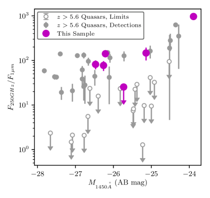
Figure 1: Selection of ultraviolet-faint, far infrared-luminous quasars based on absolute magnitude (rest-frame 1450Å) and observed sub-mm to near-infrared flux ratio. Our sample of six quasars is denoted by magenta circles, with detections for the five IR-luminous quasars, and an upper limit for the additional quasar SDSS J0005-0006. Other $z>5.6$ quasars with sub-mm observations are plotted in gray (Fan et al. 2000, 2001, 2003, 2004, 2006b; Petric et al. 2003; Bertoldi et al. 2003; Mahabal et al. 2005; Cool et al. 2006; McGreer et al. 2006; Goto 2006; Venemans et al. 2007, 2013; Wang et al. 2007, 2008, 2011, 2013; Kurk et al. 2007, 2009; Willott et al. 2007, 2010a, 2010b; Jiang et al. 2007b, 2008, 2009; Mortlock et al. 2009, 2011; Zeimann et al. 2011; De Rosa et al. 2011, 2014; Omont et al. 2013; Bañados et al. 2014; Wu et al. 2015).

Although the FIR emission suggests the presence of significant dust in the host galaxies, the quasar discovery spectra (rest-frame UV) do not show anomalous features compared to the rest of the population—i.e., they are otherwise normal $z\simeq{}{6}$ quasars, rather than showing significant spectral reddening or absorption features such as present in the FIRST/2MASS sample at lower redshifts (Urrutia et al. 2008; Glikman et al. 2015). Furthermore, more than $\sim 25\%$ of $z\simeq{}{6}$ quasars have similarly high FIR luminosities (Willott et al. 2007; Wang et al. 2008, 2010, 2011), so these FIR-luminous quasars are broadly representative of a significant sub-population, rather than atypical objects.

2.2 Dust-Free Quasar

In addition to the FIR-luminous quasars described above, we also analyze data from the prototype hot-dust-free quasar SDSS J0005–0006 (Fan et al. 2004; Jiang et al. 2010), which also lacks cold dust (Wang et al. 2008). With a lower-luminosity and no evidence for significant dust content, this quasar was selected as a counterpoint to SDSS J1148+5251. This source is representative of a smaller, but still important sub-population. At $5.8<z<6.4$, Jiang et al. (2010) found two apparently dust-free quasars in a sample of 21 quasars, or $\approx 10\%$ of the population. Leipski et al. (2014) also found that $\approx 15\%$ of their sample of 69 quasars at $z>5$ are deficient in (but not devoid of) hot dust, and there is evidence of a trend toward higher dust-poor fraction with increasing redshift (Jun & Im 2013).

Table 1: Quasars Observed with HST

Quasar Name	Redshift	$M_{1450}$ (mag)	$L_{FIR}$ $(10^{12}~{}L_{\odot{}}{})$	$\log(M_{BH}/M_{\odot})$
CFHQS J003311.40–012524.9	6.13	$-25.14$	$2.6\pm{}0.8$	$9.52\pm{}0.87^{a}$
SDSS J012958.51–003539.7	5.78	$-23.89$	$5.2\pm{}0.9$	$8.23\pm{}0.45^{b}$
SDSS J020332.39+001229.3	5.72	$-26.26$	$4.4\pm{}1.1$	$10.72\pm{}0.26^{a}$
NDWFS J142516.30+325409.0	5.89	$-26.47$	$5.4\pm{}1.2$	$9.41\pm{}0.11^{a}$
SDSS J205406.42–000514.8	6.04	$-26.21$	$5.5\pm{}1.2$	$8.95\pm{}0.47^{b}$
SDSS J000552.34–000655.8	5.85	$-25.73$	$<3.4$	$8.02^{c}$

Note. — Quasar names include the full sexagesimal coordinates. Redshifts and absolute magnitudes use the same references as Table 7 in Bañados et al. (2016). FIR luminosities are from Wang et al. (2010, 2011). Black hole masses are from $a$) Shen et al. (2019), $b$) Wang et al. (2013)/Willott et al. (2015) and $c$) Trakhtenbrot et al. (2017), and are calculated using the MgII line where available, else with the CIV line (NDWFS-J1425+3254) or by assuming the black hole is accreting at the Eddington luminosity (SDSS J0129-0035 and SDSS J2054-0005).

3 Hubble Space Telescope Data and Observing Strategy

Each of the six quasars was observed with the HST WFC3 infrared channel in the F125W (J-band) and F160W (H-band) filters. The five FIR-luminous quasars were observed for two orbits (4800 s) in each filter, while SDSS J0005–0006 was observed for four orbits (10400 s) in each filter. Windhorst et al. (2011) provides details on the WFC3 IR two-orbit sensitivity.

In addition to the quasar observations, coeval observations of a nearby PSF reference star were completed along with each epoch of quasar imaging. Although the HST PSF is stable compared to ground-based observatories, slight changes in the position of the secondary mirror cause small time-dependent focus variations. These variations are believed to be caused primarily by changes in the spacecraft thermal environment (Bély et al. 1993; Hershey 1998; Cox & Niemi 2011). We mitigated this effect by imposing constraints on the PSF star observations, as in the pilot program (Mechtley et al. 2012)—the (non-binary) stars were selected to be within $5\arcdeg{}$ of the quasar, to minimize differences in the solar illumination angle, and the stars were observed in the orbit immediately following the quasar observations, to best match the orbital day/night cycle. The HST flight calendar builders also attempted, where possible, to schedule our quasar and PSF observations immediately after an HST target from a different program in a similar part of the sky as our quasar, so as to further mitigate differences in orbital thermal variations between our first and subsequent orbits on that quasar and PSF target. This special request was possible to schedule for some of our quasars. PSF star exposures were alternated in F125W and F160W to fully sample the focal variation within an orbit (for details, see Mechtley et al. 2012). Additionally, the stars were selected to have ($J-H$) colors similar to the quasars, since the diffraction-limited PSF also varies with wavelength. In wide filters, redder sources can have a measurably broader PSF than bluer sources.

Four exposures were taken in each orbit of quasar and PSF star observations, using the four-point box sub-pixel dither pattern to improve PSF sampling and assist in the rejection of bad pixels and cosmic rays. Critically-sampled images were reconstructed using astrodrizzle, following approaches similar to those described in Koekemoer et al. (2002, 2011, 2013), with a linear pixel scale of $0\farcs{}06$ (a spatial scale of $\approx 0.36$ kpc at $z\simeq 6$) and a pixfrac parameter of 0.8, to reduce correlated noise while maintaining a relatively uniform weighting per-pixel. We used “ERR” (inverse variance) weighting for the final image combination step. We transformed the ERR extensions from the HST exposures to per-pixel RMS error maps that include all sources of error, including shot noise, and account for correlated noise, as in Casertano et al. (2000) and Dickinson et al. (2004), using astroRMS.

4 Source Modeling and Point Source Subtraction

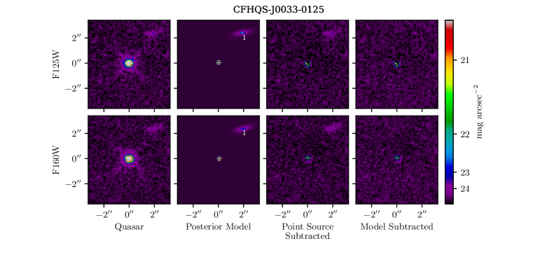
Figure 2: Posterior-weighted model images for CFHQS J0033–0125. All images show a $\approx 6\farcs 5\times 6\farcs 5$ FOV around the quasar, in order to see any companion galaxies, and are displayed with the same arcsinh color stretch and $0\farcs 060$ pixel scale. Top row: F125W filter. Bottom row: F160W filter. First column: drizzled, undistorted WFC3 images. Second column: posterior-weighted models from the MCMC fitting process, before convolution with the PSF. Third column: residual after subtracting only the point source model from the original image. Fourth column: residual after subtracting the point source model and all modeled companions from the original image. Any galaxies surrounding the quasar are indicated with a white number, for ease of comparison with Figs. 7 and 9 and Table 3.

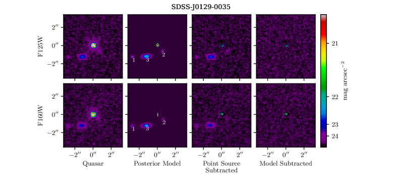
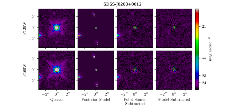
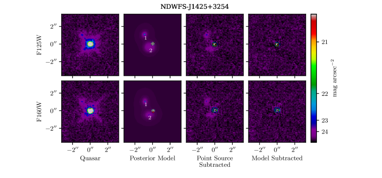
Figure 3: Posterior-weighted model images for SDSS J0129–0035, SDSS J0203+0012 and NDWFS J1425+3254. See Figure 2 for details.

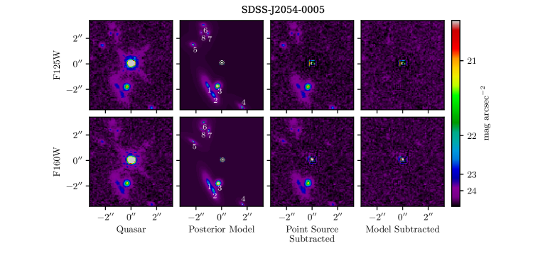
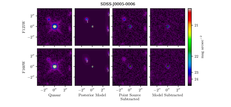
Figure 4: Posterior-weighted model images for SDSS J2054–0005 and SDSS J0005–0006. See Figure 2 for details.

We performed 2D surface brightness modeling for each quasar using the publicly available MCMC-based software psfMC (Mechtley 2014; Mechtley et al. 2016). psfMC allows the user to model an input image using a combination of point sources and Sérsic profiles (Sérsic 1963, 1968) with the parameters: sky background; point source magnitude and position; and Sérsic magnitude, position, Sérsic index $n$, effective radius of the major axis $R_{e}$, ratio between the major and minor axes $b/a$, and position angle. The MCMC process explores a range of model parameters specified by input prior probability distributions, convolving each model with an input PSF and comparing it with the telescope image, to determine the posterior probability distribution of model parameters given the observed data. The software uses the emcee ensemble sampler (Foreman-Mackey et al. 2013), which improves sampling efficiency compared to the pyMC (Patil et al. 2010) version that was used in Mechtley (2014).

For each image of each source, we attempted two different models—one with both a point source and an underlying Sérsic profile, and one with only a point source. We compared the results of the two models both visually and using the Bayesian Information Criterion as a model selection heuristic. In all cases, there was no evidence that the data required the additional Sérsic profile—the seven additional free parameters were primarily fitting noise peaks rather than residual flux from the hosts.

For all further analysis, we model the quasar as a pure point source. We also model any surrounding galaxies within $\approx 3^{\prime\prime}$ of the quasar with a Sérsic profile. It should be stressed, however, that if the galaxies are associated with the quasar and undergoing a merger, their rest-frame UV emission need not be distributed in anything like a Sérsic profile. Rather, this approach is simply used to model their flux to avoid over-subtraction. We assume uniform priors over a reasonable range, for all of the model parameters. For each quasar image, we run the MCMC with 200 chains, and a minimum of 10,000 iterations with the first 5,000 discarded as a burn-in period (systems with more surrounding galaxies required up to twice as many iterations to obtain convergence). To ensure that the model is well-fit to the data, we examine the resulting posterior distributions, altering the allowed parameter range and iteration count until each parameter has converged and the residual flux in the model subtracted image is consistent with random noise.

For the six quasars and their companion galaxies, we create posterior-weighted model images before convolution with the PSF, and after the model has been convolved with the PSF and subtracted from the original image. These weighted images are the (per-pixel) mean of all sample images, with more probable locations in parameter space being more densely populated with samples. The resulting images for the six quasars in the J- and H-bands are shown in Figures 2–4. The residual images show a central core of flux, which contains some residual flux from the quasar, and may also contain underlying host emission. The regions in the residual images where companion galaxy models have been subtracted purely consists of noise, demonstrating that the psfMC model fits the observations superbly and our observations are noise-limited.

psfMC also outputs the ‘best’ parameter values from the maximum posterior model, alongside their errors. These values for the companion galaxy fits are given in Table 3.

5 Results

5.1 Quasar Host Galaxies

5.1.1 Magnitude Limits

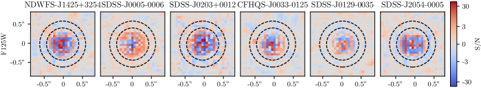
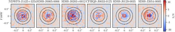
Figure 5: Residual images showing the central regions of the quasars after PSF subtraction. The deep red and blue regions show pixels with formal $S/N$ with large absolute value, artifacts of the quasar subtraction technique which caused significant pixel-to-pixel variations in the residual flux. The two circles shown in each image have radii of $0\farcs 42$ and $0\farcs 60$, which are used when performing photometry of the underlying quasar host emission.

The formal signal-to-noise ratio ($S/N$) of the residual flux in the core of each quasar after PSF-subtraction is presented in Figure 5. This central region includes residual flux from the core of the quasar PSF, caused by an imperfect match of profiles of the quasar and empirical PSF used for subtraction, alongside any potential host galaxy flux. While the total flux is subtracted correctly, with a median residual consistent with zero, the pixel-to-pixel variation of the PSFs results in pixels with residual flux that is significantly larger than expected by the noise map, with formal signal-to-noise ratios of up to $\left|S/N\right|\simeq 30$. In other words, the subtraction technique produces considerable residuals in the inner region. We note that significant quasar over- or under-subtraction is unlikely as this would produce negative or positive residuals in the diffraction spikes, respectively, which are not visible.

To estimate the flux of the host without including this contaminated inner region, we instead measure the surface brightness in annuli from 7 to 10 pixels, or 0$\farcs$42–0$\farcs$60. We choose an inner radius of 7 pixels, as this is where the pixel-to-pixel variations of the $S/N$ first reach the expected/background level. This approach ignores the central core, while including enough pixels to make a reasonable detection if any flux was present. For all quasars in both filters, no significant flux detection could be made in these annuli. The 2$\sigma$ surface brightness limits in these annuli, from the noise of each image, are given in Table 2.

To obtain the total magnitude limit of a given host, we consider a range of Sérsic profiles, with a distribution of $n$ and $R_{e}$ guided by $z\simeq 6$ observations (Shibuya et al. 2015), and take a Monte Carlo approach to determine the most likely magnitude limit given the surface brightness limit in the annulus (see Appendix A). The 2$\sigma$ magnitude limits obtained by this method are given in Table 2, with the J- and H-band limits ranging from 22.7–23.1 mag and 22.4–22.9 mag, respectively.

Table 2: Quasar Host Galaxy Detection Limits

Quasar Name	$SB_{J}$, $2\sigma$ limit ($0\farcs 42$-$0\farcs 60$)	$m_{J}$, 2$\sigma$ limit (Sérsic fit)	$SB_{H}$, $2\sigma$ limit ($0\farcs 42$-$0\farcs 60$)	$m_{H}$, 2$\sigma$ limit (Sérsic fit)
	(AB mag/′′2)	(AB mag)	(AB mag/′′2)	(AB mag)
CFHQS-J0033-0125	$24.6$	$22.9$	$24.4$	$22.7$
SDSS-J0129-0035	$24.5$	$22.8$	$24.3$	$22.6$
SDSS-J0203+0012	$24.4$	$22.7$	$24.2$	$22.4$
NDWFS-J1425+3254	$24.7$	$22.9$	$24.4$	$22.7$
SDSS-J2054-0005	$24.6$	$22.9$	$24.4$	$22.7$
SDSS-J0005-0006	$24.8$	$23.1$	$24.6$	$22.9$

5.1.2 Stellar Mass Limits

Measuring the redshift evolution of the black hole–stellar mass relation is of key importance for understanding the co-evolution of black holes and their host galaxies. Relative to the well-studied and accurately measured local relation (see, e.g., the review of Kormendy & Ho 2013), at higher redshifts observations suggest that black holes are more massive compared to their hosts. For example, at $z\simeq 1.5$ Ding et al. (2020) find a black hole–stellar mass ratio that is 2.7 times larger than the local relation, while at $z\simeq 2$, Peng et al. (2006) find a black hole–bulge mass relation 3–6 times larger. At higher redshifts, existing observations of luminous $z\simeq 6$ quasars with ALMA generally find black hole to dynamical mass ratios that are significantly larger than the local relation (e.g. Maiolino et al. 2007; Riechers et al. 2008; Venemans et al. 2012; Wang et al. 2013). However, many studies claim that high observed relations are a result of selection effects, (Lauer et al. 2007; Schulze & Wisotzki 2011, 2014; DeGraf et al. 2015; Willott et al. 2017; Ding et al. 2020). ALMA observations of lower-luminosity $z\simeq 6$ quasars indeed find these to lie on or below the local relation (Willott et al. 2017; Izumi et al. 2018, 2019).

To investigate the black hole–stellar mass relation using our HST observations, we convert our host magnitude limits to limits on stellar mass. We calculate UV slopes $\beta$ of the hosts by fitting the relation $m=-2.5\log(\lambda^{\beta+2})+m_{0}$, equivalent to $f_{\lambda}\propto\lambda^{\beta}$, to the two host magnitude limits $m_{J}$ and $m_{H}$ at $\lambda=1.25$ and 1.6 $\mu$m respectively. Using this relation and the determined $\beta$ and $m_{0}$, we calculate the UV apparent magnitude limit $m_{\mathrm{UV}}$ as that at rest-frame 1500Å, or $\lambda=(1+z)\times 0.15\mu$m. We convert this to an absolute magnitude using $M_{\mathrm{UV}}=m_{\mathrm{UV}}-DM+2.5\log(1+z)$ where $DM$ is the distance modulus.

We adopt the $z=6$ $M_{\ast}-M_{\mathrm{UV}}$ relation derived by Song et al. (2016) using a large sample of galaxies from the Cosmic Assembly Near-infrared Deep Extragalactic Legacy Survey (CANDELS)/Great Observatories Origins Deep Survey (GOODS) fields and the Hubble Ultra Deep Field (HUDF):

$$\log(M_{\ast})=9.53\pm 0.02-(0.50\pm 0.03)\times(M_{\mathrm{UV}}+21)$$ (1)

with a scatter of 0.36 dex. We use a Monte Carlo technique, sampling from a uniform distribution of magnitudes ranging from $M_{\mathrm{UV}}=-20$ mag to our $2\sigma$ upper limit for each quasar host. The lower luminosity limit of $M_{\mathrm{UV}}=-20$ mag was chosen as this is as faint as high-redshift quasar hosts are expected to be from the BlueTides simulation (Feng et al. 2015; Marshall et al. 2019, see Figure 12). We assign a stellar mass to each sampled magnitude using Equation 1, given a normal distribution with $\sigma=0.36$ dex, to determine the resulting probability distribution of stellar masses. These stellar masses are normally-distributed, so we adopt the 2$\sigma$ upper limit from this relation as our host mass limit. We note that this results in a lower, less pessimistic limit than simply taking the $2\sigma$ upper mass limit at the $2\sigma$ magnitude limit, which is very conservative.

We present the black hole–stellar mass relation from the stellar mass limits of our $z\simeq 6$ quasar hosts in Figure 6. Our limits are consistent with the black hole–stellar mass relation from existing sub-mm observations of $z\simeq 6$ quasars, (Willott et al. 2017; Izumi et al. 2018, 2019; Pensabene et al. 2020), which measure the dynamical mass of the host using gas dynamics as probed by the [CII] line, and assume $M_{\ast}=M_{\textrm{dyn}}$. Three of our quasars have dynamical mass measurements (Wang et al. 2010; Pensabene et al. 2020), which we also show in Figure 6. Our stellar mass upper limit for SDSS J2054-0005 lies above the measured dynamical mass of $M_{\textrm{dyn}}=0.7\begin{subarray}{c}+4.5\\ -0.3\end{subarray}\times 10^{10}M_{\odot}$ (Pensabene et al. 2020), suggesting that either our limit is significantly larger than the true stellar mass, with much deeper observations required to detect the underlying stellar emission, or the measured dynamical mass underestimates the total mass of the galaxy. Our stellar mass upper limit for SDSS J0129-0035 is consistent with the lower dynamical mass limit of $M_{\textrm{dyn}}>7.8\times 10^{10}M_{\odot}$ (Pensabene et al. 2020). The lower limit on the dynamical mass for NDWFS J1425+3254 of $M_{\textrm{dyn}}>1.56\times 10^{11}M_{\odot}$ (Wang et al. 2010) is larger than our stellar mass upper limit, suggesting that we are close to detecting the stellar component of this quasar host galaxy.

The stellar mass limits of five of our six quasars are consistent with the local Kormendy & Ho (2013) $M_{\ast}-M_{\mathrm{BH}}$ relation. SDSS-J0203+0012, however, has a stellar mass of $M_{\ast}<1.89\times 10^{11}M_{\odot}$, lower than expected by the local relation, given its extremely large black hole mass of $M_{\mathrm{BH}}=5.2\times 10^{10}M_{\odot}$ (Table 1, Shen et al. 2019). However, we note that this black hole mass is determined by the C IV line, as the more robust Mg II line is not covered by ground-based observations. SDSS-J0203+0012 is a broad absorption line (BAL) quasar (Mortlock et al. 2009) and so the dynamics probed by the C IV line are likely affected by the outflows. Hence we place no significance on our black hole–stellar mass relation limit for this object.

The $M_{\ast}-M_{\mathrm{UV}}$ relation is derived from observations of UV-selected galaxies, and might not apply if our hosts were dusty star-forming or quiescent galaxies; as these galaxies may be particularly dusty, our mass limits would be underestimates. Mid-infrared observations to allow for detailed SED fitting, using the upcoming James Webb Space Telescope (JWST), for example, are necessary to accurately determine the stellar masses of these potentially dusty host galaxies.

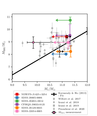
Figure 6: The black hole–stellar mass relation for our $z\simeq 6$ quasar host galaxies, alongside other $z\simeq 6$ quasars from the literature (Willott et al. 2017; Izumi et al. 2018, 2019; Pensabene et al. 2020). Existing dynamical mass measurements/limits are shown with black errorbars, for NDWFS J1425+3254 (red; Wang et al. 2010), SDSS J2054-0005 (pink; Pensabene et al. 2020) and SDSS J0129-0035 (orange; Pensabene et al. 2020). Also shown is the $z=0$ relation of Kormendy & Ho (2013), for comparison.

5.2 The Prevalence of Close, Blue Neighbors

Table 3: Properties of Galaxies Surrounding the Quasars

Quasar Name	Galaxy	$m_{J}$	$m_{J}-m_{H}$	RA	Dec	Projected Distance	Sérsic index	$R_{e}$	$b/a$	$M_{1500}$	UV slope
		(AB mag)	(AB mag)			(kpc)	$n$	(kpc)		(AB mag)	$\beta$
CFHQS-J0033-0125	1$\dagger$	$24.7\pm 0.1$	$0.1\pm 0.1$	0:33:11.519	-1:25:23.56	$17.6\pm 0.1$	$2.2\pm 0.8$	$2.9\pm 0.5$	$0.31\pm 0.08$	$-22.1\pm 0.2$	$-1.7\pm 0.6$
SDSS-J0129-0035	1*	$26.6\pm 0.3$	$0.8\pm 0.3$	1:29:58.088	-0:35:45.30	$18.6\pm 0.2$	$5.5\pm 1.7$	$1.1\pm 0.4$	$0.64\pm 0.35$	$-19.4\pm 0.5$	$1.5\pm 1.6$
	2*	$25.9\pm 0.2$	$-0.7\pm 0.2$	1:29:58.179	-0:35:42.23	$5.3\pm 0.2$	$5.2\pm 1.8$	$1.7\pm 0.4$	$0.65\pm 0.23$	$-21.4\pm 0.4$	$-4.9\pm 1.4$
	3*	$24.1\pm 0.0$	$0.1\pm 0.0$	1:29:58.114	-0:35:43.81	$10.7\pm 0.1$	$0.5\pm 0.0$	$1.9\pm 0.1$	$0.46\pm 0.03$	$-22.6\pm 0.1$	$-1.6\pm 0.2$
SDSS-J0203+0012	1a*	$23.3\pm 0.1$	$0.1\pm 0.1$	2:03:31.865	0:12:25.09	$21.3\pm 0.1$	$0.5\pm 0.0$	$1.8\pm 0.0$	$0.22\pm 0.02$	$-23.8\pm 0.3$	$-1.7\pm 1.3$
	1b*	$24.1\pm 0.1$	$-0.1\pm 0.3$	2:03:31.860	0:12:24.98	$22.1\pm 0.1$	$2.1\pm 0.7$	$1.6\pm 0.3$	$0.76\pm 0.20$	-	-
	2	$26.6\pm 0.2$	$0.2\pm 0.3$	2:03:31.883	0:12:28.62	$15.9\pm 0.3$	$4.2\pm 2.0$	$1.6\pm 0.4$	$0.57\pm 0.29$	$-19.9\pm 0.4$	$-1.1\pm 1.6$
	3	$26.2\pm 0.3$	$0.2\pm 0.3$	2:03:32.180	0:12:25.94	$16.0\pm 0.2$	$4.7\pm 1.9$	$1.8\pm 0.5$	$0.59\pm 0.31$	$-20.3\pm 0.5$	$-1.2\pm 1.6$
NDWFS-J1425+3254	1$\dagger$	$24.6\pm 0.1$	$0.4\pm 0.1$	14:25:16.767	32:54:06.98	$8.4\pm 0.1$	$3.6\pm 0.7$	$2.6\pm 0.4$	$0.81\pm 0.21$	$-21.8\pm 0.2$	$-0.4\pm 0.8$
	2*	$24.4\pm 0.1$	$0.1\pm 0.1$	14:25:16.733	32:54:05.49	$3.4\pm 0.2$	$0.5\pm 0.0$	$2.7\pm 0.1$	$0.94\pm 0.07$	$-22.3\pm 0.2$	$-1.6\pm 0.6$
SDSS-J2054-0005	1*	$23.7\pm 0.1$	$0.0\pm 0.1$	20:54:06.075	-0:05:18.12	$12.3\pm 0.1$	$1.7\pm 0.2$	$4.2\pm 0.2$	$0.39\pm 0.04$	$-23.1\pm 0.1$	$-2.2\pm 0.4$
	2*	$24.3\pm 0.1$	$0.4\pm 0.1$	20:54:06.028	-0:05:17.48	$15.6\pm 0.1$	$0.9\pm 0.2$	$2.2\pm 0.2$	$0.49\pm 0.05$	$-22.1\pm 0.1$	$-0.1\pm 0.4$
	3*	$23.3\pm 0.0$	$0.1\pm 0.0$	20:54:06.080	-0:05:17.31	$11.1\pm 0.0$	$1.6\pm 0.1$	$0.7\pm 0.0$	$0.81\pm 0.03$	$-23.5\pm 0.0$	$-1.6\pm 0.1$
	4*	$24.8\pm 0.2$	$-0.6\pm 0.1$	20:54:05.998	-0:05:15.14	$22.7\pm 0.0$	$5.7\pm 1.0$	$2.3\pm 0.4$	$0.41\pm 0.15$	$-22.5\pm 0.3$	$-4.6\pm 0.9$
	5$\dagger$	$24.9\pm 0.1$	$0.2\pm 0.1$	20:54:06.265	-0:05:19.87	$15.7\pm 0.0$	$7.0\pm 0.8$	$2.2\pm 0.5$	$0.63\pm 0.24$	$-21.7\pm 0.2$	$-1.1\pm 0.8$
	6$\dagger$	$25.1\pm 0.1$	$0.4\pm 0.1$	20:54:06.376	-0:05:19.41	$19.4\pm 0.1$	$4.6\pm 0.8$	$3.7\pm 0.4$	$0.72\pm 0.13$	$-21.4\pm 0.2$	$-0.2\pm 0.8$
	7$\dagger$	$25.3\pm 0.2$	$0.4\pm 0.2$	20:54:06.336	-0:05:18.94	$14.8\pm 0.0$	$5.6\pm 0.9$	$1.7\pm 0.2$	$0.55\pm 0.11$	$-21.1\pm 0.3$	$-0.2\pm 1.1$
	8	$26.0\pm 0.2$	$0.4\pm 0.2$	20:54:06.334	-0:05:19.44	$16.7\pm 0.0$	$4.8\pm 0.8$	$2.2\pm 0.4$	$0.56\pm 0.16$	$-20.5\pm 0.3$	$-0.5\pm 1.1$
SDSS-J0005-0006	1a*	$25.1\pm 0.1$	$-0.3\pm 0.3$	0:05:52.046	-0:06:59.94	$10.8\pm 0.1$	$0.7\pm 0.2$	$1.0\pm 0.1$	$0.85\pm 0.10$	$-22.1\pm 0.6$	$-1.8\pm 2.1$
	1b*	$25.7\pm 0.3$	$0.5\pm 0.2$	0:05:52.038	-0:06:59.83	$9.8\pm 0.2$	$6.4\pm 1.2$	$2.0\pm 0.9$	$0.59\pm 0.45$	-	-
	2*	$25.7\pm 0.1$	$0.7\pm 0.4$	0:05:52.217	-0:06:56.57	$23.5\pm 0.1$	$5.7\pm 1.5$	$2.7\pm 0.6$	$0.41\pm 0.16$	$-20.4\pm 0.4$	$1.0\pm 1.7$
	3$\dagger$	$25.4\pm 0.1$	$0.0\pm 0.2$	0:05:52.032	-0:06:55.61	$17.3\pm 0.1$	$2.1\pm 0.9$	$2.6\pm 0.5$	$0.33\pm 0.11$	$-21.3\pm 0.3$	$-2.0\pm 0.9$

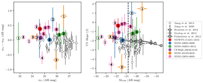
Figure 7: Left: J-H color vs. J-band magnitude and Right: Rest-frame UV slope $\beta$ vs. 1500 Å absolute magnitude, measured for each of the galaxies within $\simeq 3^{\prime\prime}$ of our six quasars, assuming they are at the same redshift as the quasar. Filled colored circles show those with colors and magnitudes consistent with $z\sim 6$ galaxies, while open colored circles show candidates which are likely to be foreground interlopers given their colors and magnitudes. The numerical labels correspond to labels in the individual quasar images (Figures 2-4), and Table 3, for ease of comparison. Grey symbols represent spectroscopically-confirmed $z\simeq 6$ galaxies from Jiang et al. (2013, 2020) and the average relations for dropout-selected LBGs from Bouwens et al. (2012), Dunlop et al. (2012), and Finkelstein et al. (2012) (see legend). The dashed black line shows the value of $M^{*}$ (Finkelstein 2016).

Figures 2–4 reveal that all of our six quasars have neighboring galaxies within the surrounding $6\farcs 5\times 6\farcs 5$. For SDSS-J0129-0035, NDWFS-J1425+3254 and SDSS-J0005-0006, some companions overlap with the quasar PSF, highlighting the need for the quasar PSF subtraction in order to fully understand the local quasar environment.

The properties of these 20 neighboring galaxies from the maximum posterior model found by psfMC are listed in Table 3. We calculate their UV magnitudes and slopes following the same procedure as for the host galaxies (see Section 5.1.2). The magnitudes and colors of these galaxies are displayed in Figure 7, along with samples of star-forming galaxies at $z\simeq 6$. Four of these companions have colors/UV-slopes that are too red ($\beta>0$) or too blue ($\beta<-4$) to be consistent with $z\simeq 6$ galaxies. In addition, seven galaxies are too bright to be likely at this redshift, with magnitudes brighter than $M_{\mathrm{UV}}=-22.1$ mag, the magnitude of the brightest spectroscopically-confirmed $z\simeq 6$ galaxy in the sample of Finkelstein et al. (2015). The remaining 9 companion galaxies—surrounding five of our six quasars—have UV magnitudes and slopes consistent with those of star-forming galaxies at $z\simeq 6$. The majority of these are brighter than $M^{\ast}$ ($-20.79$ mag at $z=6$, Finkelstein 2016, see Table 3). Unfortunately, existing observations at sub-mm to radio wavelengths do not resolve and/or detect the individual sources (e.g. Wang et al. 2013), so morphological comparisons with existing data are not possible.

These 9 potential companion galaxies are separated from the quasars by $1\farcs 4$–$3\farcs 2$, corresponding to projected distances of 8.4–19.4 kpc. Simulations show that galaxies with companions at similar separations have higher AGN fractions (McAlpine et al. 2020), and also enhanced star formation rates (Patton et al. 2020). This suggests that these companions, if their true 3D distance is of order their projected distance, could be interacting with the quasar host galaxies and may potentially have triggered or enhanced the observed AGN activity. However, tidal features from any such interaction would likely be rendered invisible due to the $(1+z)^{4}$ surface brightness dimming at $z\simeq 6$.

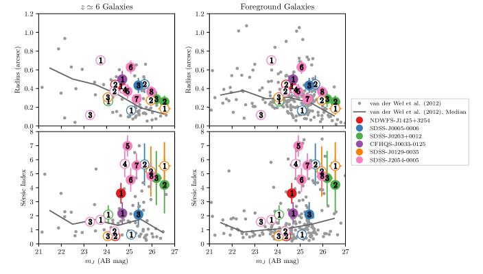
Figure 8: The morphological properties measured for each of the galaxies within $3^{\prime\prime}$ of our 6 quasars. Top row: effective radius $R_{e}$ vs. J-band magnitude. Bottom row: Sérsic index $n$ vs. J-band magnitude. Filled colored circles show those with colors and magnitudes consistent with $z\simeq 6$ galaxies, while open colored circles show candidates which are likely to be foreground interlopers given their colors and magnitudes. The numerical labels correspond to labels in the individual quasar images (Figures 2-4), and Table 3, for ease of comparison. Also shown are measurements of galaxy sizes in the CANDELS GOODS-South survey from van der Wel et al. (2012), for comparison. Left panel: van der Wel et al. (2012) galaxies with best estimate redshift $z>5.5$, and a 95 per cent confidence that $z>5$. Right panel: Galaxies within $3^{\prime\prime}$ of these $z>5.5$ galaxies, at any redshift. Grey dots show individual galaxies, and the grey line shows the median in bins of 1 magnitude.

We examine the relationship between size, Sérsic index and magnitude for these neighboring galaxies in Figure 8, in comparison to $z\simeq 6$ galaxies in the CANDELS GOODS-South sample (van der Wel et al. 2012; Brammer et al. 2012; Skelton et al. 2014; Momcheva et al. 2016). This shows that our companion galaxy sizes are as large as the largest $z\simeq 6$ CANDELS field galaxies, but are larger than the median size of $z\simeq 6$ field galaxies by an average of $0\farcs 1$. Their Sérsic profiles are as steep as the steepest Sérsic indexes of CANDELS $z\simeq 6$ field galaxies, but are larger than the median Sérsic index of $z\simeq 6$ field galaxies by an average of 2. Thus, our potential quasar companion galaxies have morphological parameters that are consistent with the larger and steeper-Sérsic CANDELS $z\simeq 6$ field galaxies. Similar conclusions are made when comparing our potential companion galaxies to neighbors within $3^{\prime\prime}$ of $z\simeq 6$ galaxies in the CANDELS GOODS-South sample (Figure 8, van der Wel et al. 2012), of which the majority (95%) are foreground objects at $z<5.5$. Our potential companions have sizes and Sérsic indices that are larger than the median of the neighbors of $z\simeq 6$ CANDELS galaxies, although their properties are reasonably consistent with the more massive neighbors. Hence, based on their size and Sérsic distributions we cannot determine whether our observed neighbors are more likely to be $z\simeq 6$ galaxies than foreground interlopers.

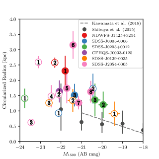
Figure 9: The circularized effective radius $R_{e}\sqrt{b/a}$ vs. 1500 Å absolute magnitude measured for each of the galaxies within $3^{\prime\prime}$ of our 6 quasars, assuming they are at the same redshift as the quasar. Filled colored circles show those with colors and magnitudes consistent with $z\sim 6$ galaxies, while open colored circles show candidates which are likely to be foreground interlopers given their colors and magnitudes. The numerical labels correspond to labels in the individual quasar images (Figures 2-4), and Table 3, for ease of comparison. The size–luminosity relations from the high-redshift observations of Shibuya et al. (2015) and Kawamata et al. (2018) are also shown, for comparison.

We show the relationship between size and UV absolute magnitude for these potential companion galaxies in Figure 9, assuming they are at the same redshift as the quasar. Our objects that have UV magnitudes and slopes consistent with $z\simeq 6$ galaxies lie on a relatively tight size-luminosity relation. This relation is fairly consistent with, but somewhat higher than, that of $z\simeq 6$ Lyman-break galaxies measured by Shibuya et al. (2015) (for galaxies with $-22\lesssim M_{\textrm{UV}}\lesssim-18$ mag) and Kawamata et al. (2018) (for galaxies with $-21.5\lesssim M_{\textrm{UV}}\lesssim-12$ mag), with our objects having larger sizes at the same luminosities.

We note that the measured sizes of galaxies may be affected by systematic differences between these studies. For example, the treatment of the sky background in the fitting can have a significant impact on the resulting Sérsic fit parameters (see, e.g., Guo et al. 2009; Bruce et al. 2012). We include the background level as a free parameter in the MCMC-fitting, which can result in larger values of $R_{e}$ and Sérsic index $n$ than if the background level is fixed (Bruce et al. 2012), potentially contributing to some of the discrepancy between our results and those of Shibuya et al. (2015), who assume a fixed background level. Bruce et al. (2012) show that there is a positive correlation between measured $R_{e}$ and Sérsic index $n$. Shibuya et al. (2015) assume $n=1.5$ for Lyman-break galaxies, and Kawamata et al. (2018) fix $n=1$. As our fitting method finds larger Sérsic indices for our potential $z\simeq 6$ companion galaxies, with a mean of $n=4.3$, this correlation may explain, at least in part, our larger measured sizes.

Using the number of galaxies observed in HST data of comparable depth (WFC3 ERS2 field, $m_{H}<26.5$; Windhorst et al. 2011, see their figure 12), the average number of galaxies observed is $\approx 373,000$ per square degree, or 0.0288 objects per square arcseconds, if galaxies are uniformly distributed on the sky. We thus expect to find on average 7.3 random foreground objects within our six $\approx 6\farcs 5\times 6\farcs 5$ quasar images (total area $\approx 250$ square arcseconds; Figures 2–4), at $z\ll 6$ and unrelated to our quasars. The surface density variations in these numbers due to foreground cosmic variance and photometric zeropoint errors is expected to be $\lesssim$15% in the H-band (see, e.g., figure 3 of Driver et al. 2016), so we would on average expect $\lesssim$ 8.4 random foreground objects at $z\ll 6$.

Assuming that the galaxy neighbor distribution follows a Poisson distribution, the probability of observing a total of 20 galaxies within the $\approx 250$ square arcsecond area, $4\sigma$ above the expected value of 8.4 foreground galaxies, is $\lesssim 0.0003$. Hence, given the unlikelihood that so many galaxies would be found by chance, it is probable that some of these objects are physically associated with the quasars. Of the 20 close neighbors, 11 have UV magnitudes and slopes that suggest that they are unlikely to be at $z\simeq 6$. Finding these 11 foreground galaxies is consistent within $1\sigma$ of these Poisson expectations. The remaining 9 neighbors have UV magnitudes and slopes consistent with known $z\simeq 6$ galaxies. We will adopt this number of 9 potential quasar companion galaxies in our discussion below, however we note that the true number of $m_{J}<26.5$ $z\simeq 6$ companion galaxies in our images could be between 0 and 20, with 9 a more reasonable upper limit on the expected number based on the above arguments.

In Figure 10 we plot the average number of potential $z\simeq 6$ companion galaxies found in our quasar fields, compared to expectations for number counts of $z=6$ galaxies in random fields (Finkelstein et al. 2015). We see significant excess compared to expectations of random pointings, with our average of $\sim$1.5 galaxies within 0.13 cMpc of the quasars ($3\farcs 2$ at $z=6$) higher than the expected number of 0.0056 galaxies, corresponding to an overdensity of a factor of $\sim$270. This large excess is similar to the overdensity found by Decarli et al. (2017, see their figure 3b), who detected 4 companion galaxies in [CII] with ALMA around 4 of 25 $z\gtrsim 6$ quasars.

Decarli et al. (2017) find that their measured overdensity is consistent with measurements of quasar–Lyman break galaxy clustering at $z\simeq 4$ (García-Vergara et al. 2017), when applied to the [CII] luminosity function. We consider the models of the $z\simeq 4$ García-Vergara et al. (2017) quasar–galaxy clustering and the $z=5.9$ galaxy–galaxy clustering of Qiu et al. (2018) to account for this effect, and find that our measurement is consistent with both clustering models applied to the Finkelstein et al. (2015) luminosity function. Thus, as with the Decarli et al. (2017) sample, our observed potential $z\simeq 6$ companion counts can be explained by expectations for high-redshift galaxy clustering. Hence, while we find that our quasars are in environments that are more dense than the average field density, with an overdensity of a factor of $\sim$270, they are in similar environments to that expected for a typical luminous $z\simeq 6$ field galaxy. In fact, if we have overestimated the number of true companion galaxies at 9, then our quasars may be in somewhat less dense regions than the typical luminous $z\simeq 6$ galaxy

While Decarli et al. (2017) had a secure number of $z\simeq 6$ companions from ALMA [CII] redshifts, we present a consistent upper limit from the number of possible $z\simeq$6 companions following the above arguments. Clearly, JWST integral field redshifts, ALMA [CII] redshifts, or VLT MUSE redshifts would be needed to determine the real number of companion galaxies around our quasars, and their overdensity compared to the field at $z\simeq$6.

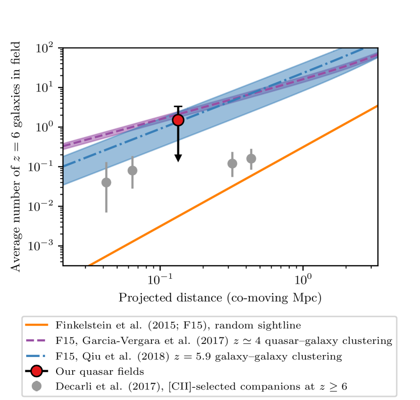
Figure 10: The average number of potential $z\simeq 6$ companion galaxies found within $3\farcs 2$ (0.13 cMpc) of our six quasars, compared with expectations for counts of $z=6$ galaxies in random fields from the Finkelstein et al. (2015) luminosity function, as a function of projected distance from the quasar. We consider a cylindrical volume centred on the quasar with depth $\Delta z=1$. Errors on our observation show the range of 1–20 true $z\simeq 6$ companions, around our best estimate of 9, where 20 is the total number of objects found within $3\farcs 2$ of our six quasars; the lower error is marked with an arrow to account for the (unlikely) limiting case that none of the neighboring galaxies are true $z\simeq 6$ companions. Also shown are the observations of $z\geq 6$ quasar companions of Decarli et al. (2017), for comparison. We also plot the Finkelstein et al. (2015) luminosity function predictions modified to account for the effect of large-scale clustering. We take two models for the excess in the galaxy number density $\xi(r)=(r_{0}/r)^{\gamma}$, with $r_{0}=8.83\begin{subarray}{c}+1.39\\ -1.51\end{subarray}h^{-1}$ cMpc and $\gamma=2.0$ from the quasar–Lyman break galaxy clustering of $z=4$ galaxies measured by García-Vergara et al. (2017), and $r_{0}=5.3\begin{subarray}{c}+2.3\\ -2.6\end{subarray}h^{-1}$ cMpc and $\gamma=1.6$ from the galaxy–galaxy clustering measurements of $z=5.9$ $M_{UV}<-19.99$ galaxies (Qiu et al. 2018).

5.2.1 Additional Observations of NDWFS-J1425+3254

The quasar NDWFS-J1425+3254 shows further evidence for having close companions. The discovery spectrum of Cool et al. (2006) shows a significant absorption feature at roughly $8350$ Å,  $20$ Å  red-ward of Lyman-$\alpha$. This line could potentially be caused by HI absorption from a companion galaxy infalling at $720\textrm{~{}km~{}s}^{-1}$ (Mechtley 2014). By assuming the system is virialized and that the companion is at a projected distance of 4.8 kpc, Mechtley (2014) find that this corresponds to a dynamical mass of $\sim 5.8\times 10^{11}M_{\odot}$. Using the Song et al. (2016) $M_{\ast}-M_{\mathrm{UV}}$ relation (Equation 1), from our detection limits the host of NDWFS-J1425+3254 has a stellar mass of $M_{\ast}<2.0\times 10^{11}M_{\odot}$, with the two companions having masses of $\sim 7.8\times 10^{8}M_{\odot}$ and $\sim 1.3\times 10^{9}M_{\odot}$. The properties of the CO $(6-5)$ line (Wang et al. 2010) provide independent evidence for a group-like gravitational potential; the line fit gives a FWHM of $690\pm 180$ km s^-1, and the peak of the emission is redshifted ($z={5.89}$) from the reported Ly$\alpha$ redshift ($z={5.85}$, Cool et al. 2006).

To further investigate this system, we obtained observations with the Large Binocular Camera (LBC) on the Large Binocular Telescope (LBT) in the $g$-, $r$-, and $i$-bands (Fig 11). No LBC $g$-band flux is detected in a $2\farcs 0$ aperture to a limit of $m_{g}\gtrsim 28.3$ mag, with Lyman-Werner flux from the quasar detected in the $r$-band at $m_{r}=24.7$ mag. Even in decent seeing conditions ($\approx 0\farcs 8-1\farcs 0$) the ground-based PSF of the quasar has broad wings that significantly affect the detection limit of close companions out to 2$\farcs$0 or greater (see, e.g., Ashcraft et al. 2018). A best-effort point-source subtraction results in an upper limit of $m_{r}\gtrsim 25.7$ mag for the more distant of the two companions. The J- and H-band detections but faint $g$- and $r$-band limits are sufficient to exclude the possibility that these companions are blue foreground galaxies, but not that they could be red luminous galaxies at $z\simeq 1.1$. Additional observations are therefore required to confirm that these ‘companion’ galaxies are indeed at $z\simeq 6$, and not foreground interlopers.

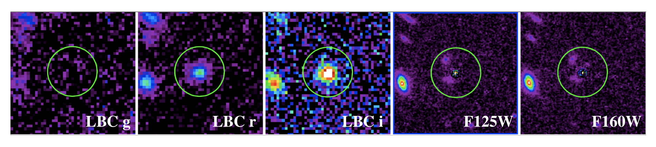
Figure 11: Thumbnail images of NDWFS-J1425+3254. From left to right: LBT/LBC $g$-, $r$-, and $i$-bands, and HST WFC3 IR J- and H-bands. The companion galaxies are visible within the green circle of radius $2\farcs 0$ in the point source-subtracted WFC3 IR images. Lyman-$\alpha$ emission from the quasar at $\simeq 8330$Å  is captured by the $i$-band image, while Lyman-Werner flux from the quasar is bright enough to be seen in the $r$-band, even in these LBT observations (see the discovery spectrum of Cool et al. 2006). Due to the seeing of the ground-based images, estimated as $\simeq 0\farcs 8-1\farcs 0$ FWHM, point source subtraction on the $r$-band LBC image produces an inconclusive upper limit for the combined companion galaxy flux.

6 Discussion

6.1 The Dust Content of Quasar Hosts

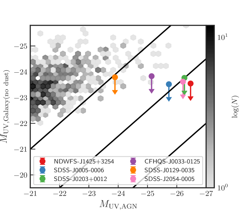
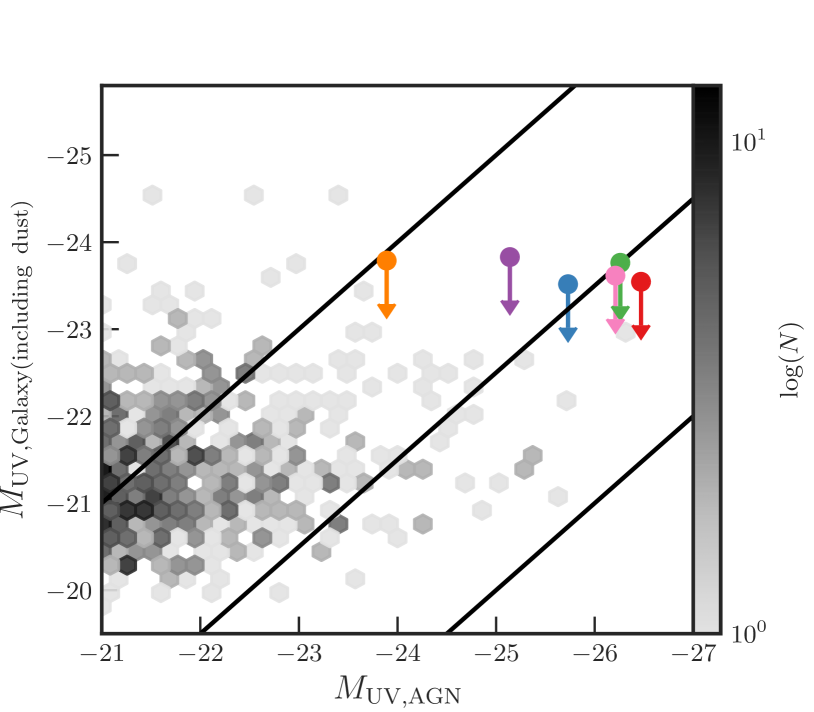
Figure 12: The relation between quasar and host galaxy UV-luminosity for our sample (colored upper limits; see legend) and for the simulated $z=7$ quasars from the BlueTides simulation (grey density plots). The left panel shows the BlueTides host galaxies’ intrinsic UV-luminosities, while the right panel shows them after dust attenuation, which is calculated using the density of gas in the simulation (see Ni et al. 2019; Marshall et al. 2019). Diagonal black lines show where the ratio of quasar to host brightness is 1:1, 10:1 and 100:1.

To understand the magnitude limits and dust properties of our quasar host galaxies, we consider the sample of $z=7$ quasars in the BlueTides simulation (Feng et al. 2015). BlueTides is a large-scale cosmological hydrodynamical simulation, which models the evolution of $2\times 7040^{3}$ particles in a cosmological box of volume $(400/h~{}\rm{cMpc})^{3}$ from initial conditions at $z=99$ to $z=7$, the lowest published redshift to date (Marshall et al. 2019; Ni et al. 2019). Figure 12 presents the relation between galaxy and quasar UV luminosity, for our observations and the BlueTides quasars. Both the intrinsic and dust-attenuated galaxy magnitudes for the BlueTides galaxies are shown, with the dust attenuation of galaxies modeled in BlueTides using the density of metals along a line of sight (for full details, see Marshall et al. 2019). From the BlueTides simulation, we find that hosts of $M_{\mathrm{UV}}<-23$ mag quasars at $z=7$ have between 1.4 to 3.8 mag extinction in the UV, with an average of $A_{\mathrm{UV}}=2.6$ mag, corresponding to $A_{\mathrm{V}}=1.0$ (Calzetti et al. 2000).

From Figure 12, we see that the majority of intrinsic UV magnitudes for host galaxies of similar luminosity quasars in BlueTides are brighter than our host galaxy upper limits, with only a small percentage consistent with our limits. Given that we make no detections of all six quasar hosts, our upper limits are sufficient to rule out the possibility that our quasars are generally hosted by dust-free galaxies. Instead, our limits favour host galaxies with significant dust-attenuation, consistent with the $\langle A_{\mathrm{UV}}\rangle=2.6$ mag that is seen for the BlueTides quasar hosts (Figure 12, Marshall et al. 2019). If the BlueTides sample including dust obscuration is representative of the true $z\simeq 6$ quasar population, our upper limits are brighter than the host magnitudes that are expected, and future observations would need to probe at least $\sim 1$ mag fainter to begin to detect the host emission. We will focus on integrating BlueTides with our observational techniques to make specific predictions for upcoming JWST observations in future work.

SDSS J0005-0006 was found to be a dust-poor quasar by Jiang et al. (2013), as it was undetected with the Spitzer Space Telescope at 15.6 and 24 $\mu$m. Further observations by Leipski et al. (2014) detected the quasar with Spitzer at these wavelengths, however did not detect emission at $\geq 100\mu$m with Herschel, and so they also conclude that the quasar is deficient of hot dust compared to the majority of quasars in their sample. Non-detection of the quasar with the Max Planck Millimeter Bolometer Array (MAMBO) at 250 GHz (Wang et al. 2008) results in upper limits of the dust mass of the host of $M_{\textrm{dust}}<1.9\times 10^{8}M_{\odot}$ (Calura et al. 2014). While these observations do not detect significant amounts of dust in this system, it is still possible for some dust to be present, resulting in low-level dust attenuation of the host galaxy. Thus, while our magnitude limit for the host of SDSS J0005-0006 is fainter than the magnitudes expected of quasar hosts with no dust attenuation from the BlueTides simulation, our non-detection of the host can be reasonably explained by some minor dust attenuation in the generally dust-deficient system. Additionally, if the simulation was run to $z\simeq 6$, we would expect to see a larger sample of luminous quasars, and potentially more with host luminosities fainter than our magnitude limits, which could explain our observations. Thus, the ‘dust-free’ nature of SDSS J0005-0006 is not in significant tension with our overall dust predictions.

Our six quasars were selected in the $z$-band as $i$-band dropouts with rest-frame UV luminosities at $z\simeq 6$ of $-26.5\lesssim M_{UV}\lesssim-24$ mag (Table 1). Hence, their UV accretion disks are still, by selection, remarkably well visible. Five of our $z\simeq 6$ quasars were also selected to have significant FIR emission, and as a consequence the young stellar populations in their host galaxies are not visible in the best high dynamic range J- and H-band images that HST can produce.

We inferred that their host galaxies are likely considerably dusty ($\langle A_{\mathrm{UV}}\rangle=2.6$ mag), yet the embedded quasars are easily detected in the rest-frame UV and thus not significantly obscured (see, e.g., Vito et al. 2019). This must have significant consequences for the geometry of the small and large scale dust distribution. One possible explanation is that the embedded rapidly-accreting supermassive black hole produced a significant outflow that vacated a sufficiently large cone on scales of 10-100 pc—fortuitously aligned in our direction—that the quasar has become clearly visible at rest-frame UV wavelengths, while the host galaxy is not. Significant outflows have indeed been observed from high-redshift quasars (e.g. Alexander et al. 2010; Nesvadba et al. 2011; Maiolino et al. 2012), and are expected to be able to carve a window for observing the quasar through otherwise high-density gas (Ni et al. 2019). Thus, it seems likely that such outflows are present in these systems. These objects are therefore high priority targets for JWST, which will add 1.6–29 $\mu$m wavelength imaging coverage to our 1.2–1.6 $\mu$m HST images, and so is expected to much better constrain the dust extinction and geometry that UV images alone cannot capture.

6.2 Quasar Selection Bias

Five $z\simeq{}{6}$ quasars for this HST program were selected as those UV-faint quasars with confirmed sub-mm detections, and thus the greatest rest-frame $L_{\textrm{FIR}}/L_{\textrm{UV}}$ ratios. This selects for host systems with the greatest non-AGN contribution to the FIR flux, with inferred ultraluminous infrared galaxy (ULIRG)-class FIR luminosities ($>10^{12}~{}L_{\odot{}}{}$) and implied star formation rates of $\approx 500M_{\odot}\textrm{yr}^{-1}$ (Wang et al. 2011). Locally, ULIRGs are gas-rich with high inferred star formation rates, and most are undergoing major mergers or at least strong interactions (e.g. Howell et al. 2010; Kim et al. 2013). This suggests that this sample of $z\simeq 6$ quasars are a distinct quasar sub-population, which may be biased towards quasars with nearby interacting galaxies. This potential selection bias may mean that while our six quasars are in environments typical of luminous $z\simeq 6$ galaxies, the overall $z\simeq 6$ quasar population may reside in somewhat under-dense environments. However, note that Trakhtenbrot et al. (2017b) observed three FIR-bright and three FIR-faint quasars with ALMA, finding spectroscopically confirmed sub-mm companion galaxies interacting with three quasars—one FIR-bright and two FIR-faint. We also find a potential companion around SDSS J0005-0006, which is not detected in the FIR (Wang et al. 2008; Jiang et al. 2013; Leipski et al. 2014). Hence, companion galaxies are not necessarily a feature of only FIR-bright quasars.

This selection bias is also likely to affect the measured black hole–stellar mass relation, as these quasars are not necessarily representative of the overall $z\simeq 6$ quasar population. For example, the most highly star-forming quasar host galaxies in BlueTides show a significantly steeper black hole–stellar mass relation, with such quasars lying on the main relation for the most massive black holes, and below the relation for lower-mass black holes. This result suggests that our ULIRG-type hosts, which are also selected to be UV-faint and thus potentially have lower mass black holes, may lie below the black hole–stellar mass relation of the full quasar population.

The bias to selecting ULIRG-class host galaxies may also affect our stellar mass limits, as these galaxies generally lie significantly above the SFR–stellar mass main sequence. Their extreme star-formation rates may indicate the presence of large amounts of dust extinction, as discussed in Section 6.1, which could further bias our measurements.

6.3 The Prevalence of $z\simeq 6$ Quasars with Companions

Companion galaxies have been discovered around a range of high-redshift quasars, with the majority seen only in observations at sub-mm wavelengths (e.g. Wagg et al. 2012; Decarli et al. 2017). For example, Trakhtenbrot et al. (2017a, b) found companions physically associated with three of six $z\simeq 4.8$ quasars observed with ALMA, at separations of 14-45 kpc. Those companions have dynamical masses $M_{\textrm{dyn}}=(2.1-10.7)\times 10^{10}M_{\ast}$, compared with the quasar hosts which have $M_{\textrm{dyn}}=(3.7-7.4)\times 10^{10}M_{\ast}$, indicative of major galaxy interactions. These companion galaxies are not detected in Spitzer data, and so Trakhtenbrot et al. (2017b) conclude that there must be significant dust-obscuration. This result may explain the lack of companions observed in rest-frame UV observations (e.g. Willott et al. 2005); this is supported by simulations (Marshall et al. 2019).

Our potential companion galaxies are detected in the rest-frame UV, suggesting that these companions may have less dust attenuation than those observed in the sub-mm. Other studies have also observed companions in the rest-frame UV; for example, McGreer et al. (2014) discovered a companion galaxy around both a $z=4.9$ and a $z=6.25$ quasar, at 5 and 12 kpc projected separations. While the companion of the $z=4.9$ quasar is spectroscopically confirmed, the $z=6.25$ companion is presumed to be at that redshift based on imaging in two HST filters, as in our study. While identifying these two companions, McGreer et al. (2014) reported that bright companions around high-redshift quasars are uncommon, with an incidence of $\lesssim 2/29$ for $\gtrsim 5L^{\ast}$ galaxies and $\lesssim 1/6$ for $2\lesssim L\lesssim 5L^{\ast}$ galaxies.

Finding quasar companion galaxies is consistent with the scenario that the growth of high-redshift quasars is triggered by galaxy mergers. While simulations predict that galaxy mergers can fuel quasar activity, it is unclear if these are the dominant cause of high-redshift black hole growth. For example, using the EAGLE simulation, McAlpine et al. (2018) reported that at $z=0$, $\sim 60\%$ of black holes undergoing a rapid growth phase do so within $\pm 0.5$ dynamical times of a galaxy-galaxy merger, and McAlpine et al. (2020) found an over-abundance of AGN within merging systems relative to control samples of inactive or isolated galaxies. However, while galaxies experiencing mergers have two to three times higher accretion rates than isolated galaxies, the majority of black hole mass growth does not occur during the merger periods (McAlpine et al. 2020). Thus, if the potential companions are confirmed to be associated with our $z\simeq 6$ quasars, this result may be due to our biased sample of FIR-luminous quasars (see discussion in Section 6.2) and not necessarily indicative that nearby companions are common around high-redshift quasars.

7 Summary

We use Hubble Space Telescope imaging of five far infrared-luminous $z\simeq 6$ quasars, and the hot-dust free quasar SDSS J0005-0006, to search for rest-frame UV emission from their host galaxies. Using the Markov Chain Monte Carlo estimator psfMC, we perform 2D surface brightness modeling for each quasar to model and subtract the quasar point source in order to detect possible underlying host emission.

Only upper limits were found for the quasar host galaxies, of $m_{J}>22.7$ and $m_{H}>22.4$ mag. These limits are beginning to probe magnitudes expected for high-redshift quasar hosts from the BlueTides simulation, which suggests that the increased resolution and near–mid-infrared spectroscopic capability of the James Webb Space Telescope (JWST) should detect host emission in the rest-frame UV/optical for the first time (see also the BlueTides predictions of Marshall et al. 2019). We also expect that these host galaxies could be quite dusty, with $\langle A_{\mathrm{UV}}\rangle\simeq 2.6$ mag (see Figure 12), and thus probing their mid-infrared emission with JWST will be invaluable.

Converting these magnitude limits to stellar mass limits suggests that five of the six quasars could be consistent with the local black hole–stellar mass relation of Kormendy & Ho (2013), and with existing sub-mm observations of $z\simeq 6$ quasar hosts (Willott et al. 2017; Izumi et al. 2018, 2019; Pensabene et al. 2020). SDSS-J0203+0012 has a stellar mass of $\log(M_{\ast}/M_{\odot})<11.28$ and a large black hole mass of $\log(M_{\textrm{BH}}/M_{\odot})=10.72$, which places it above the local relation. However, its black hole mass is likely inaccurate.

We detect up to nine potential $z\simeq 6$ companion galaxies surrounding five of the six quasars, with magnitudes and UV spectral slopes consistent with luminous $z\simeq 6$ star-forming galaxies. These galaxies lie within $1\farcs 4$–$3\farcs 2$ of the quasars, or at a projected distance of 8.4–19.4 kpc (if at the same redshift). If their true distance is of order their projected distance, these companions could be interacting with the quasar host galaxies, potentially enhancing their quasar activity (McAlpine et al. 2020; Patton et al. 2020). Finding nine potential $z\simeq 6$ companion galaxies is consistent with expectations for large-scale clustering around high-redshift quasars (García-Vergara et al. 2017) and galaxies (Qiu et al. 2018, see Figure 10). Hence, we find that our quasars are in environments typical of luminous $z\simeq 6$ galaxies.

The existing data cannot rule out the probability that some of these potential companions are foreground interlopers. Future observations will focus on better constraining the spectral energy distributions of the companions, including deep $r$-band imaging to identify low-redshift interlopers, and adaptive optics-corrected K-band imaging to better constrain the rest-frame UV SED. The launch of the JWST will allow spectroscopic measurements of the redshifts of these potential companion galaxies, determining whether they are indeed physically associated with the quasars, and perhaps being high-redshift major mergers in progress.

Appendix A Magnitude Calculation

To convert the surface brightness in the annulus 0$\farcs$42–0$\farcs$60 to a magnitude, we consider the host galaxy to have a Sérsic profile and to be azimuthally symmetric. The total flux contained within radius $R$ is

$$F(R)=\int_{0}^{R}2\pi rf(r)dr$$ (A1)

where $f(r)$ is the flux per unit physical area at radius $r$. For a Sérsic profile with Sérsic index $n$ and effective radius $R_{e}$,

$$f(r)=f(R_{e})\exp\left(-b_{n}\left((r/R_{e})^{1/n}-1\right)\right)$$ (A2)

where $b_{n}$ is defined to satisfy $\Gamma(2n)=2\gamma(2n,b_{n})$, where $\Gamma$ and $\gamma$ are the complete and incomplete gamma functions, $\Gamma(a)=\int_{0}^{\infty}t^{a-1}e^{-t}dt$ and $\gamma(a,x)=\int_{0}^{x}t^{a-1}e^{-t}dt$. Thus, $F(R)$ can be expressed as

$$F(R)=2\pi R_{e}^{2}f(R_{e})~{}ne^{b_{n}}b_{n}^{-2n}~{}\gamma(2n,b_{n}(R/R_{e})^{1/n}).$$ (A3)

Given $\Delta F=F(0\farcs 60)-F(0\farcs 42)$ is the flux measured in the annulus, $f(R_{e})$ can be calculated from:

$$f(R_{e})=\Delta F\left[2\pi R_{e}^{2}ne^{b_{n}}b_{n}^{-2n}~{}\left[\gamma(2n,x_{1})-\gamma(2n,x_{2})\right]\right]^{-1}$$ (A4)

where $x_{1}=b_{n}(0.60/R_{e}\textrm{[arcsec]})^{1/n}$ and $x_{2}=b_{n}(0.42/R_{e}\textrm{[arcsec]})^{1/n}$. We thus calculate the flux of the host galaxy as $F(0\farcs 60)$.

We calculate this flux for a range of Sérsic profiles, with $n\in(0.5,5)$ and $R_{e}\in(0,4)$ kpc, ignoring galaxies which have magnitudes brighter than the observed magnitude of the quasar. We show an example for the J-band magnitude of NDWFS-J1425+3254 in Figure 13.

Guided by the observations of $z\simeq 6$ bright (1–10$L^{\ast}_{z=3}$), massive galaxies by Shibuya et al. (2015), we assume probability distribution functions for $n$ and $R_{e}$, with the combined 2D probability distribution function shown in Figure 13. We use a Monte Carlo technique to sample from this distribution, and determine the resulting probability distribution function for host galaxy magnitude. We choose the most-likely value from this distribution as our magnitude limit. Note that this is not the magnitude of the most likely $n$-$R_{e}$ combination, as many less-likely $n$-$R_{e}$ combinations produce similar magnitudes and make those more likely.

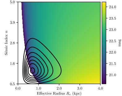
Figure 13: The J-band magnitude of the host galaxy of NDWFS-J1425+3254, as an example, assuming a Sérsic profile with Sérsic index $n$ and effective radius $R_{e}$ that is constrained to have the measured flux (a $2\sigma$ noise limit) in the annulus 0$\farcs$42–0$\farcs$60. We show a range of Sérsic profiles, with $n\in(0.5,5)$ and $R_{e}\in(0,4)$ kpc. The white regions show galaxies with magnitudes brighter than the quasar itself (here $m_{J}<20.6$), which we exclude. The black contours show the 2D probability distribution functions for $n$ and $R_{e}$, guided by the observations of $z\simeq 6$ bright (1–10$L^{\ast}_{z=3}$), massive galaxies by Shibuya et al. (2015), assuming the parameters are independent. Using a Monte Carlo technique to sample magnitudes from this distribution gives a magnitude probability distribution function, from which we choose the most likely value as the corresponding magnitude limit, in this case $m_{J}>22.8$ mag.

References

- Alexander et al. (2010) Alexander, D. M., Swinbank, A. M., Smail, I., McDermid, R., & Nesvadba, N. P. H. 2010, MNRAS, 402, 2211
- Ashcraft et al. (2018) Ashcraft, T. A., Windhorst, R. A., Jansen, R. A., et al. 2018, PASP, 130, 064102
- Astropy Collaboration et al. (2013) Astropy Collaboration, Robitaille, T. P., Tollerud, E. J., et al. 2013, A&A, 558, A33
- Bahcall et al. (1994) Bahcall, J. N., Kirhakos, S., & Schneider, D. P. 1994, AJ, 435, L11
- Bañados et al. (2013) Bañados, E., Venemans, B., Walter, F., et al. 2013, ApJ, 773, 178
- Bañados et al. (2014) Bañados, E., Venemans, B. P., Morganson, E., et al. 2014, AJ, 148, 14
- Bañados et al. (2016) Bañados, E., Venemans, B. P., Decarli, R., et al. 2016, ApJS, 227, 11
- Bañados et al. (2017) Bañados, E., Venemans, B. P., Mazzucchelli, C., et al. 2017, arXiv e-prints, arXiv:1712.01860
- Barth et al. (2003) Barth, A. J., Martini, P., Nelson, C. H., & Ho, L. C. 2003, ApJL, 594, L95
- Bély et al. (1993) Bély, P. Y., Hasan, H., & Miebach, M. 1993, Orbital Focus Variations in the Hubble Space Telescope, Instrument Science Report SESD-1993-16, STScI, Baltimore
- Bertoldi et al. (2003) Bertoldi, F., Carilli, C. L., Cox, P., et al. 2003, A&A, 406, L55
- Bouwens et al. (2004) Bouwens, R. J., Illingworth, G. D., Blakeslee, J. P., Broadhurst, T. J., & Franx, M. 2004, The Astrophysical Journal, 611, L1
- Bouwens et al. (2012) Bouwens, R. J., Illingworth, G. D., Oesch, P., et al. 2012, ApJ, 754, 83
- Brammer et al. (2012) Brammer, G. B., van Dokkum, P. G., Franx, M., et al. 2012, The Astrophysical Journal Supplement Series, 200, 13
- Bruce et al. (2012) Bruce, V. A., Dunlop, J. S., Cirasuolo, M., et al. 2012, Monthly Notices of the Royal Astronomical Society, 427, 1666
- Calura et al. (2014) Calura, F., Gilli, R., Vignali, C., et al. 2014, MNRAS, 438, 2765
- Calzetti et al. (2000) Calzetti, D., Armus, L., Bohlin, R. C., et al. 2000, ApJ, 533, 682
- Casertano et al. (2000) Casertano, S., de Mello, D., Dickinson, M., et al. 2000, The Astronomical Journal, 120, 2747
- Cisternas et al. (2011) Cisternas, M., Jahnke, K., Inskip, K. J., et al. 2011, ApJ, 726, 57
- Cool et al. (2006) Cool, R. J., Kochanek, C. S., Eisenstein, D. J., et al. 2006, AJ, 132, 823
- Cox & Niemi (2011) Cox, C., & Niemi, S.-M. 2011, Evaluation of a temperature-based HST focus model, Instrument Science Report TEL 2011-01, STScI, Baltimore
- Davies et al. (2018) Davies, F. B., Hennawi, J. F., Bañados, E., et al. 2018, ApJ, 864, 142
- De Rosa et al. (2011) De Rosa, G., Decarli, R., Walter, F., et al. 2011, ApJ, 739, 56
- De Rosa et al. (2014) De Rosa, G., Venemans, B. P., Decarli, R., et al. 2014, ApJ, 790, 145
- Decarli et al. (2017) Decarli, R., Walter, F., Venemans, B. P., et al. 2017, Nature, 545, 457
- DeGraf et al. (2015) DeGraf, C., Matteo, T. D., Treu, T., et al. 2015, Monthly Notices of the Royal Astronomical Society, 454, 913
- Dickinson et al. (2004) Dickinson, M., Stern, D., Giavalisco, M., et al. 2004, ApJL, 600, L99
- Ding et al. (2020) Ding, X., Silverman, J., Treu, T., et al. 2020, The Astrophysical Journal, 888, 37
- Disney et al. (1995) Disney, M. J., Boyce, P. J., Blades, J. C., et al. 1995, Nature, 376, 150
- Driver et al. (2016) Driver, S. P., Andrews, S. K., Davies, L. J., et al. 2016, The Astrophysical Journal, 827, 108
- Dunlop et al. (2003) Dunlop, J. S., McLure, R. J., Kukula, M. J., et al. 2003, MNRAS, 340, 1095
- Dunlop et al. (2012) Dunlop, J. S., McLure, R. J., Robertson, B. E., et al. 2012, MNRAS, 420, 901
- Fan et al. (2000) Fan, X., White, R. L., Davis, M., et al. 2000, AJ, 120, 1167
- Fan et al. (2001) Fan, X., Narayanan, V. K., Lupton, R. H., et al. 2001, AJ, 122, 2833
- Fan et al. (2003) Fan, X., Strauss, M. A., Schneider, D. P., et al. 2003, AJ, 125, 1649
- Fan et al. (2004) Fan, X., Hennawi, J. F., Richards, G. T., et al. 2004, AJ, 128, 515
- Fan et al. (2006a) Fan, X., Strauss, M. A., Becker, R. H., et al. 2006a, AJ, 132, 117
- Fan et al. (2006b) Fan, X., Strauss, M. A., Richards, G. T., et al. 2006b, AJ, 131, 1203
- Feng et al. (2015) Feng, Y., Di-Matteo, T., Croft, R. A., et al. 2015, MNRAS, 455, 2778
- Finkelstein (2016) Finkelstein, S. L. 2016, PASA, 33, e037
- Finkelstein et al. (2012) Finkelstein, S. L., Papovich, C., Ryan, R. E., et al. 2012, ApJ, 758, 93
- Finkelstein et al. (2015) Finkelstein, S. L., Ryan, Jr., R. E., Papovich, C., et al. 2015, ApJ, 810, 71
- Floyd et al. (2013) Floyd, D. J. E., Dunlop, J. S., Kukula, M. J., et al. 2013, MNRAS, 429, 2
- Foreman-Mackey (2016) Foreman-Mackey, D. 2016, The Journal of Open Source Software, 24, doi:10.21105/joss.00024
- Foreman-Mackey et al. (2013) Foreman-Mackey, D., Hogg, D. W., Lang, D., & Goodman, J. 2013, Publications of the Astronomical Society of the Pacific, 125, 306
- García-Vergara et al. (2017) García-Vergara, C., Hennawi, J. F., Barrientos, L. F., & Rix, H.-W. 2017, The Astrophysical Journal, 848, 7
- Glikman et al. (2015) Glikman, E., Simmons, B., Mailly, M., et al. 2015, ApJ, 806, 218
- Goto (2006) Goto, T. 2006, MNRAS, 371, 769
- Greig & Mesinger (2017) Greig, B., & Mesinger, A. 2017, MNRAS, 465, 4838
- Greig et al. (2019) Greig, B., Mesinger, A., & Bañados, E. 2019, MNRAS, 484, 5094
- Guo et al. (2009) Guo, Y., McIntosh, D. H., Mo, H. J., et al. 2009, Monthly Notices of the Royal Astronomical Society, 398, 1129
- Hershey (1998) Hershey, J. L. 1998, Modelling HST Focal-Length Variations, Instrument Science Report SESD-1997-01, STScI, Baltimore
- Hopkins et al. (2006) Hopkins, P. F., Hernquist, L., Cox, T. J., et al. 2006, ApJS, 163, 1
- Howell et al. (2010) Howell, J. H., Armus, L., Mazzarella, J. M., et al. 2010, ApJ, 715, 572
- Hunter (2007) Hunter, J. D. 2007, Computing in Science & Engineering, 9, 90
- Hutchings (2003) Hutchings, J. B. 2003, AJ, 125, 1053
- Izumi et al. (2018) Izumi, T., Onoue, M., Shirakata, H., et al. 2018, PASJ, 70
- Izumi et al. (2019) Izumi, T., Onoue, M., Matsuoka, Y., et al. 2019, PASJ, 71
- Jiang et al. (2020) Jiang, L., Cohen, S. H., Windhorst, R. A., et al. 2020, ApJ, 889, 90
- Jiang et al. (2007a) Jiang, L., Fan, X., Ivezić, Ž., et al. 2007a, ApJ, 656, 680
- Jiang et al. (2007b) Jiang, L., Fan, X., Vestergaard, M., et al. 2007b, AJ, 134, 1150
- Jiang et al. (2008) Jiang, L., Fan, X., Annis, J., et al. 2008, AJ, 135, 1057
- Jiang et al. (2009) Jiang, L., Fan, X., Bian, F., et al. 2009, AJ, 138, 305
- Jiang et al. (2010) Jiang, L., Fan, X., Brandt, W. N., et al. 2010, Nature, 464, 380
- Jiang et al. (2013) Jiang, L., Egami, E., Mechtley, M., et al. 2013, ApJ, 772, 99
- Jun & Im (2013) Jun, H. D., & Im, M. 2013, ApJ, 779, 104
- Kawamata et al. (2015) Kawamata, R., Ishigaki, M., Shimasaku, K., Oguri, M., & Ouchi, M. 2015, The Astrophysical Journal, 804, 103
- Kawamata et al. (2018) Kawamata, R., Ishigaki, M., Shimasaku, K., et al. 2018, ApJ, 855, 4
- Kim et al. (2013) Kim, D.-C., Evans, A. S., Vavilkin, T., et al. 2013, ApJ, 768, 102
- Kim et al. (2009) Kim, S., Stiavelli, M., Trenti, M., et al. 2009, ApJ, 695, 809
- Kocevski et al. (2012) Kocevski, D. D., Faber, S. M., Mozena, M., et al. 2012, ApJ, 744, 148
- Koekemoer et al. (2002) Koekemoer, A. M., Fruchter, A. S., Hook, R. N., & Hack, W. 2002, in The 2002 HST Calibration Workshop: Hubble after the Installation of the ACS and the NICMOS Cooling System (Baltimore: STScI), 337
- Koekemoer et al. (2011) Koekemoer, A. M., Faber, S. M., Ferguson, H. C., et al. 2011, ApJS, 197, 36
- Koekemoer et al. (2013) Koekemoer, A. M., Ellis, R. S., McLure, R. J., et al. 2013, ApJS, 209, 3
- Kormendy & Ho (2013) Kormendy, J., & Ho, L. C. 2013, ARA&A, 51, 511
- Kukula et al. (2001) Kukula, M. J., Dunlop, J. S., McLure, R. J., et al. 2001, MNRAS, 326, 1533
- Kurk et al. (2009) Kurk, J. D., Walter, F., Fan, X., et al. 2009, ApJ, 702, 833
- Kurk et al. (2007) —. 2007, ApJ, 669, 32
- Laporte et al. (2016) Laporte, N., Infante, L., Troncoso Iribarren, P., et al. 2016, The Astrophysical Journal, 820, 98
- Lauer et al. (2007) Lauer, T. R., Tremaine, S., Richstone, D., & Faber, S. M. 2007, The Astrophysical Journal, 670, 249
- Leipski et al. (2014) Leipski, C., Meisenheimer, K., Walter, F., et al. 2014, ApJ, 785, 154
- Mahabal et al. (2005) Mahabal, A., Stern, D., Bogosavljević, M., Djorgovski, S. G., & Thompson, D. 2005, The Astrophysical Journal, 634, L9
- Maiolino et al. (2007) Maiolino, R., Neri, R., Beelen, A., et al. 2007, A&A, 472, L33
- Maiolino et al. (2012) Maiolino, R., Gallerani, S., Neri, R., et al. 2012, MNRAS, 425, L66
- Marian et al. (2019) Marian, V., Jahnke, K., Mechtley, M., et al. 2019, ApJ, 882, 141
- Marshall et al. (2019) Marshall, M. A., Ni, Y., Matteo, T. D., et al. 2019, arXiv e-prints, 1912.03428v2
- McAlpine et al. (2018) McAlpine, S., Bower, R. G., Rosario, D. J., et al. 2018, MNRAS, 481, 3118
- McAlpine et al. (2020) McAlpine, S., Harrison, C. M., Rosario, D. J., et al. 2020, Monthly Notices of the Royal Astronomical Society, 2002.00959v2
- McGreer et al. (2006) McGreer, I. D., Becker, R. H., Helfand, D. J., & White, R. L. 2006, ApJ, 652, 157
- McGreer et al. (2014) McGreer, I. D., Fan, X., Strauss, M. A., et al. 2014, AJ, 148, 73
- McLeod & Bechtold (2009) McLeod, K. K., & Bechtold, J. 2009, ApJ, 704, 415
- McLeod & Rieke (1994) McLeod, K. K., & Rieke, G. H. 1994, ApJ, 420, 58
- Mechtley (2014) Mechtley, M. 2014, PhD Thesis, Arizona State University, Tempe, AZ, USA
- Mechtley et al. (2012) Mechtley, M., Windhorst, R. A., Ryan, R. E., et al. 2012, ApJ, 756, L38
- Mechtley et al. (2016) Mechtley, M., Jahnke, K., Windhorst, R. A., et al. 2016, ApJ, 830, 156
- Momcheva et al. (2016) Momcheva, I. G., Brammer, G. B., van Dokkum, P. G., et al. 2016, The Astrophysical Journal Supplement Series, 225, 27
- Morselli et al. (2014) Morselli, L., Mignoli, M., Gilli, R., et al. 2014, A&A, 568, A1
- Mortlock et al. (2009) Mortlock, D. J., Patel, M., Warren, S. J., et al. 2009, A&A, 505, 97
- Mortlock et al. (2011) Mortlock, D. J., Warren, S. J., Venemans, B. P., et al. 2011, Nature, 474, 616
- Nesvadba et al. (2011) Nesvadba, N. P. H., Polletta, M., Lehnert, M. D., et al. 2011, MNRAS, 415, 2359
- Ni et al. (2019) Ni, Y., Matteo, T. D., Gilli, R., et al. 2019, arXiv e-prints, 1912.03780v2
- Oesch et al. (2010) Oesch, P. A., Bouwens, R. J., Carollo, C. M., et al. 2010, ApJ, 709, L21
- Oke & Gunn (1983) Oke, J. B., & Gunn, J. E. 1983, ApJ, 266, 713
- Omont et al. (2013) Omont, A., Willott, C. J., Beelen, A., et al. 2013, A&A, 552, A43
- Ono et al. (2013) Ono, Y., Ouchi, M., Curtis-Lake, E., et al. 2013, The Astrophysical Journal, 777, 155
- Pandas Development Team (2020) Pandas Development Team. 2020, pandas-dev/pandas: Pandas, v.0.23.4, Zenodo, doi:10.5281/zenodo.3509134
- Patil et al. (2010) Patil, A., Huard, D., & Fonnesbeck, C. J. 2010, J. Stat. Softw., 35, 1
- Patton et al. (2020) Patton, D. R., Wilson, K. D., Metrow, C. J., et al. 2020, Monthly Notices of the Royal Astronomical Society, 494, 4969
- Peng et al. (2010) Peng, C. Y., Ho, L. C., Impey, C. D., & Rix, H.-W. 2010, AJ, 139, 2097
- Peng et al. (2006) Peng, C. Y., Impey, C. D., Rix, H., et al. 2006, ApJ, 649, 616
- Pensabene et al. (2020) Pensabene, A., Carniani, S., Perna, M., et al. 2020, arXiv e-prints, 2002.00958v1
- Petric et al. (2003) Petric, A. O., Carilli, C. L., Bertoldi, F., et al. 2003, AJ, 126, 15
- Planck Collaboration et al. (2014) Planck Collaboration, Ade, P. A. R., Aghanim, N., et al. 2014, A&A, 571, A16
- Qiu et al. (2018) Qiu, Y., Wyithe, J. S. B., Oesch, P. A., et al. 2018, Monthly Notices of the Royal Astronomical Society, 481, 4885
- Riechers et al. (2008) Riechers, D. A., Walter, F., Brewer, B. J., et al. 2008, ApJ, 686, 851
- Sanders et al. (1988) Sanders, D. B., Soifer, B. T., Elias, J. H., et al. 1988, ApJ, 325, 74
- Schlafly & Finkbeiner (2011) Schlafly, E. F., & Finkbeiner, D. P. 2011, ApJ, 737, 103
- Schlegel et al. (1998) Schlegel, D. J., Finkbeiner, D. P., & Davis, M. 1998, ApJ, 500, 525
- Schmidt (1963) Schmidt, M. 1963, Nature, 197, 1040
- Schulze & Wisotzki (2011) Schulze, A., & Wisotzki, L. 2011, Astronomy & Astrophysics, 535, A87
- Schulze & Wisotzki (2014) —. 2014, MNRAS, 438, 3422
- Sérsic (1963) Sérsic, J. L. 1963, Boletin de la Asociacion Argentina de Astronomia La Plata Argentina, 6, 41
- Sérsic (1968) —. 1968, Atlas de Galaxias Australes
- Shen et al. (2019) Shen, Y., Wu, J., Jiang, L., et al. 2019, ApJ, 873, 35
- Shibuya et al. (2015) Shibuya, T., Ouchi, M., & Harikane, Y. 2015, ApJS, 219, 15
- Shields et al. (2006) Shields, G. A., Menezes, K. L., Massart, C. A., & Bout, P. V. 2006, ApJ, 641, 683
- Skelton et al. (2014) Skelton, R. E., Whitaker, K. E., Momcheva, I. G., et al. 2014, ApJS, 214, 24
- Song et al. (2016) Song, M., Finkelstein, S. L., Ashby, M. L. N., et al. 2016, ApJ, 825, 5
- Targett et al. (2012) Targett, T. A., Dunlop, J. S., & McLure, R. J. 2012, MNRAS, 420, 3621
- Trakhtenbrot et al. (2017a) Trakhtenbrot, B., Lira, P., Netzer, H., et al. 2017a, ApJ, 836, 8
- Trakhtenbrot et al. (2017b) —. 2017b, Frontiers in Astronomy and Space Sciences, 4, 49
- Trakhtenbrot et al. (2017) Trakhtenbrot, B., Volonteri, M., & Natarajan, P. 2017, ApJ, 836, L1
- Urrutia et al. (2008) Urrutia, T., Lacy, M., & Becker, R. H. 2008, ApJ, 674, 80
- Valiante et al. (2014) Valiante, R., Schneider, R., Salvadori, S., & Gallerani, S. 2014, MNRAS, 444, 2442
- van der Walt et al. (2011) van der Walt, S., Colbert, S. C., & Varoquaux, G. 2011, Computing in Science & Engineering, 13, 22
- van der Wel et al. (2012) van der Wel, A., Bell, E. F., Häussler, B., et al. 2012, The Astrophysical Journal Supplement Series, 203, 24
- Venemans et al. (2007) Venemans, B. P., McMahon, R. G., Warren, S. J., et al. 2007, MNRAS, 376, L76
- Venemans et al. (2012) Venemans, B. P., McMahon, R. G., Walter, F., et al. 2012, ApJ, 751, L25
- Venemans et al. (2013) Venemans, B. P., Findlay, J. R., Sutherland, W. J., et al. 2013, ApJ, 779, 24
- Villforth et al. (2018) Villforth, C., Herbst, H., Hamann, F., et al. 2018, MNRAS, 483, 2441
- Virtanen et al. (2020) Virtanen, P., Gommers, R., Oliphant, T. E., et al. 2020, Nature Methods, 17, 261
- Vito et al. (2019) Vito, F., Brandt, W. N., Bauer, F. E., et al. 2019, A&A, 1906.04241v2
- Volonteri (2012) Volonteri, M. 2012, Science, 337, 544
- Wagg et al. (2012) Wagg, J., Wiklind, T., Carilli, C. L., et al. 2012, ApJ, 752, L30
- Wang et al. (2007) Wang, R., Carilli, C. L., Beelen, A., et al. 2007, AJ, 134, 617
- Wang et al. (2008) Wang, R., Carilli, C. L., Wagg, J., et al. 2008, ApJ, 687, 848
- Wang et al. (2010) Wang, R., Carilli, C. L., Neri, R., et al. 2010, ApJ, 714, 699
- Wang et al. (2011) Wang, R., Wagg, J., Carilli, C. L., et al. 2011, AJ, 142, 101
- Wang et al. (2013) —. 2013, ApJ, 773, 44
- Willott et al. (2015) Willott, C. J., Bergeron, J., & Omont, A. 2015, ApJ, 801, 123
- Willott et al. (2017) —. 2017, ApJ, 850, 108
- Willott et al. (2005) Willott, C. J., Percival, W. J., McLure, R. J., et al. 2005, ApJ, 626, 657
- Willott et al. (2007) Willott, C. J., Delorme, P., Omont, A., et al. 2007, AJ, 134, 2435
- Willott et al. (2010a) Willott, C. J., Albert, L., Arzoumanian, D., et al. 2010a, AJ, 140, 546
- Willott et al. (2010b) Willott, C. J., Delorme, P., Reylé, C., et al. 2010b, AJ, 139, 906
- Windhorst et al. (2011) Windhorst, R. A., Cohen, S. H., Hathi, N. P., et al. 2011, ApJS, 193, 27
- Wu et al. (2015) Wu, X.-B., Wang, F., Fan, X., et al. 2015, Nature, 518, 512
- Zeimann et al. (2011) Zeimann, G. R., White, R. L., Becker, R. H., et al. 2011, ApJ, 736, 57