Detecting Dark Energy Fluctuations with Gravitational Waves

Abstract

Luminosity distance estimates from electromagnetic and gravitational wave sources are generally different in models of dynamical dark energy and gravity beyond the standard cosmological scenario. We show that this leaves a unique imprint on the angular power-spectrum of fluctuations of the luminosity distance of gravitational-wave observations which tracks inhomogeneities in the dark energy field. Exploiting the synergy in supernovae and gravitational wave distance measurements, we build a joint estimator that directly probes dark energy fluctuations, providing a conclusive evidence for their existence in case of detection. Moreover, such measurement would also allow to probe the running of the Planck mass. We discuss experimental requirements to detect these signals.

I Introduction

Over the last decades, a variety of cosmological data have confirmed $\Lambda$CDM as the standard model of cosmology Aghanim et al. (2018); Abbott et al. (2018). Despite its successes, the physical nature of its main components still eludes us. In particular, understanding whether cosmic acceleration is sourced by a cosmological constant, $\Lambda$, or rather by dynamical dark energy (DE) or modifications of the laws of gravity (MG) is one of the main science drivers of upcoming cosmological missions. In the presence of DE/MG, the dynamical degrees of freedom of the theory change, generally with the appearance of a new scalar field to which we broadly refer as the “DE field”. The latter, leaves imprints not only on the dynamics of the Universe, but also on the clustering and growth of large-scale cosmological structures. Next generation galaxy surveys Amendola et al. (2018); Bacon et al. (2020); Doré et al. (2014); Ivezic et al. (2019) aim at constraining these effects and, possibly, indirectly detecting DE/MG.

The detection of gravitational waves (GW) has opened a new observational window onto our Universe, promising to offer complementary probes to shed light on cosmic expansion. GW events at cosmological distances can be used as standard sirens Schutz (1986); Holz and Hughes (2005); Cutler and Holz (2009) for measuring the expansion rate of the universe. This recent approach is complementary to measuring the luminosity distance of standard candles, like Type-Ia supernovae (SN). Multi-messenger observations can also be used to test theories of modified gravity, as recently reviewed in Ezquiaga and Zumalacárregui (2018).

On the homogeneous and isotropic background, luminosity distances depend only on redshift, leading to the standard distance-redshift relation. Inhomogeneities in the Universe induce a dependence of the distances on direction. Fluctuations in the EM luminosity distance constitute an important probe for cosmology and have been well studied Sasaki (1987); Pyne and Birkinshaw (2004); Holz and Linder (2005); Hui and Greene (2006); Bonvin et al. (2006), while the case of GWs has been addressed in General Relativity (GR) in Laguna et al. (2010); Kocsis et al. (2006); Bonvin et al. (2017); Hirata et al. (2010); Dai et al. (2017); Mukherjee et al. (2020a, b). In presence of DE/MG, the GW luminosity distance generally differs from the one traced by electromagnetic (EM) signals, both at the unperturbed, background level Belgacem et al. (2018a, b) and in its large-scale fluctuations Garoffolo et al. (2019); Dalang et al. (2019). Importantly, fluctuations in the EM luminosity distance are affected by the DE field only indirectly while, as first shown in Garoffolo et al. (2019), linearized fluctuations of the GW luminosity distance contain contributions directly proportional to the clustering of the DE field.

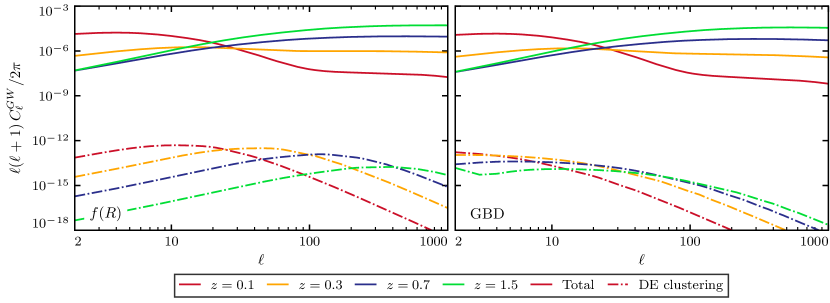
Figure 1: Angular power-spectrum of gravitational-wave luminosity distance fluctuations. Solid lines show the total power-spectrum, dashed lines the scalar field clustering component.

In this work we combine SN and GW luminosity distance fluctuations into a novel estimator to directly detect the signal of DE clustering. This signal can not be mimicked by other effects and would provide convincing evidence for the existence of the DE field. If DE does not directly couple to known particles through non-gravitational interactions, ours is a promising method to pursue its direct detection. The approach we propose allows to probe the DE field at cosmological scales, far from sources that can hide its presence by means of screening mechanisms (see e.g. Joyce et al. (2015); Babichev and Deffayet (2013); Burrage and Sakstein (2018)).

II The GW luminosity distance power-spectrum in DE/MG

The luminosity distance, as inferred by an EM or GW signal propagating through a universe with structures, depends on the observed redshift, $z$, and on the direction of arrival in the sky, $\hat{\theta}$. We decompose the observed luminosity distance of a source as a sum of its background and fluctuation components, i.e. $d_{L}(\hat{\theta},z)=\bar{d}_{L}(z)+\Delta d_{L}(\hat{\theta},z)$. We work in the context of scalar-tensor theories of gravity, which encompass most of the candidate DE/MG models. These theories are characterized by a non-minimal coupling of the DE field to space-time curvature. This causes a running of the Planck mass, $M_{P}$, which generally depends on the background configuration of the DE field $\varphi$, and on its first derivatives, through $X=-\nabla_{\mu}\varphi\nabla^{\mu}\varphi/2$. More specifically, we consider DHOST theories Langlois and Noui (2016); Crisostomi et al. (2016); Langlois et al. (2017) (see e.g. Langlois (2019)), focusing on scenarios that ensure luminal speed for GWs and avoid instabilities associated with graviton decay into DE (Crisostomi et al. (2019)). We require that high-frequency scalar fluctuations propagate at the same speed of tensor modes, as discussed in Garoffolo et al. (2019). The dependence of $M_{P}$ on the DE field gives new contributions to $d_{L}^{\rm GW}$ with respect to the GR case. At the background level one finds $\bar{d}^{\rm GW}_{L}=[M_{P}(z)/M_{P}(0)]\bar{d}_{L}$, where $\bar{d}_{L}=(1+z)\int_{0}^{z}d\tilde{z}[(1+\tilde{z})\mathcal{H}]^{-1}$ is the luminosity distance associated to electromagnetic sources, with $\mathcal{H}=a^{\prime}/a$ the Hubble parameter. The multiplicative factor $M_{P}(z)/M_{P}(0)$ accounts for the extra friction acting on the GWs during their propagation induced by the running of $M_{P}$.

At the linear level in fluctuations, generalizing to DHOST the procedure of Garoffolo et al. (2019) as shown in Appendix A, we find:

$$\frac{\Delta d^{\rm GW}_{L}}{\bar{d}^{\rm GW}_{L}}= -\kappa-(\phi+\psi)+\frac{1}{{\chi}}\int^{{\chi}}_{0}d\tilde{\chi}\,(\phi+\psi)$$

$$+\phi\bigg{(}\frac{1}{\mathcal{H}{\chi}}-\frac{M^{\prime}_{P}}{\mathcal{H}M_{P}}\bigg{)}+v_{\|}\bigg{(}1-\frac{1}{\mathcal{H}{\chi}}+\frac{M^{\prime}_{P}}{\mathcal{H}M_{P}}\bigg{)}$$

$$-\left(\,1-\frac{1}{\mathcal{H}{\chi}}+\frac{M^{\prime}_{P}}{\mathcal{H}M_{P}}\right)\int^{{\chi}}_{0}d\tilde{\chi}\,(\phi^{\prime}+\psi^{\prime})$$

$$+\frac{M_{P,\varphi}}{M_{P}}\delta\varphi+\frac{M_{P,X}}{M_{P}}\delta X\,.$$ (1)

where a prime indicates differentiation w.r.t. conformal time, $\kappa$ denotes the weak lensing convergence, $\chi$ the comoving distance to the source, $\phi$ the Newtonian potential, $\psi$ the intrinsic spatial curvature potential, and $v_{\|}$ the component along the line of sight of the peculiar velocity of the source: all in Poisson gauge and following the conventions of Garoffolo et al. (2019). $M_{P,\varphi}$ and $M_{P,X}$ stand for the derivative of $M_{P}(\varphi,X)$ w.r.t. its arguments.

The physical effects contributing to $\Delta d^{\rm GW}_{L}$ are: lensing convergence, volume dilation, and time delay in the first line of Eq. (II), that are only indirectly influenced by DE/MG; Sachs-Wolfe (SW), Doppler shifts, and Integrated Sachs-Wolfe (ISW) effects in the second and third lines, which show an additional explicit decay that depends on the evolution of $M_{P}$; damping due to DE field inhomogeneities in the fourth line of Eq. (II). These last effects are the main interest of this work as they are unique to the GW luminosity distance fluctuations.

We use Eq. (II) to build the angular power-spectrum of GW luminosity distance fluctuations averaged over a given redshift distribution of the sources

$$C^{\rm GW}_{\ell}=4\pi\int\text{d}\ln k\left(\frac{\Delta d^{\rm GW}_{L}}{\bar{d}^{\rm GW}_{L}}\right)^{W}_{k\,\ell}\left(\frac{\Delta d^{\rm GW}_{L}}{\bar{d}^{\rm GW}_{L}}\right)^{W}_{k\,\ell}\,,$$ (2)

where we work in Fourier space for the perturbations, with $k$ being the momentum, and

$$\left(\frac{\Delta d^{\rm GW}_{L}}{\bar{d}^{\rm GW}_{L}}\right)^{W}_{k\,\ell}=\int^{\infty}_{0}dz\,j_{\ell}(k\chi)\,W(z)\,\left(\frac{\Delta d^{\rm GW}_{L}}{\bar{d}^{\rm GW}_{L}}\right)\,,$$ (3)

and $j_{\ell}(x)$ is the spherical Bessel function and $W(z)$ is the source window function, normalized to $1$. The effect of each term in Eq. (II) on the angular power-spectrum can be studied independently. We report their explicit forms in Appendix C. We use the notation $\bar{d}_{L}(z)$ for the background luminosity distance, to indicate its angular average, weighted by the given redshift distribution.

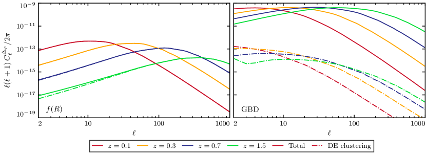
Figure 2: The angular power-spectrum of the difference between GW and SN luminosity distance fluctuations. Solid lines show the total power-spectrum, dashed lines the scalar field clustering component.

We have implemented the calculation of $C_{\ell}^{\rm GW}$ in EFTCAMB Hu et al. (2014), allowing us to study this quantity for a broad host of DE/MG models. In order to explore in detail the impact of MG on $C_{\ell}^{\rm GW}$ we focus for a moment on two representative models. First, a designer $f(R)$ model on a $\Lambda$CDM background Song et al. (2007), with the only model parameter set to $B_{0}=10^{-4}$ which is compatible with current constraints Peirone et al. (2017). Second, an agnostic parametrization of $M_{P}$, such that the ratio $(M^{\prime}_{P}/M_{P})$ is a linear function of the scale-factor, $a(z)$, $M^{\prime}_{P}/M_{P}\equiv(M^{\prime}_{P}/M_{P})|_{o}\,a$, where $(M^{\prime}_{P}/M_{P})|_{o}$ is the value of the ratio today, which we set to $0.05$. This minimal parametrization, implemented on a $\Lambda$CDM background, is representative of the Generalized Brans-Dicke (GBD) De Felice and Tsujikawa (2010); Perrotta et al. (1999); Baccigalupi et al. (2000) family. In both these models, the Planck mass $M_{P}$ depends on the scalar field value alone. We defer to future works the investigation of cases where $M_{P}$ depends also on $X$.

Figure 1 shows the angular power-spectrum, $C_{\ell}^{\rm GW}$, for the two scenarios described above. To highlight redshift dependencies, we choose a Gaussian distribution for the GW sources centred in various redshifts $z_{i}$, with width $\Delta z=0.01$, i.e. $W(z)={\cal N}\exp[-(z-z_{i})^{2}/(2\Delta z^{2})]$ where ${\cal N}$ is the normalization constant. The total signal significantly changes shape with increasing redshift. At low redshifts and large scales, the signal is dominated by the Doppler effect, due to the bulk-flow of the environment in which the GW sources are embedded. The Doppler contribution then decays for growing $\ell$, and the angular power-spectrum at small scales is dominated by lensing convergence; the Doppler term also decays in redshift, while lensing grows and eventually dominates the high-redshift part of the signal. For both models considered, the relative behaviour between Doppler and lensing convergence is qualitatively unaltered with respect to GR Bertacca et al. (2018). Figure 1 also shows the direct contribution of $\delta\varphi$ to the total signal, i.e. the last line in Eq. (II). This is of the same order of magnitude in both scenarios, and results largely subdominant compared to the total signal. For the $f(R)$ model the scalar field contribution has a noticeable scale-dependent feature that evolves in time as the Compton wavelength of the model. At higher redshift, the Compton scale of the scalar field is smaller and, correspondingly, the feature in the power-spectrum moves to smaller scales. In the GBD case, on the other hand, any feature in the shape of the power-spectrum is less pronounced, as it only leads to the decay of DE fluctuations below the horizon.

III The joint SN/GW estimator

The direct contributions of DE fluctuations to $C_{\ell}^{\rm GW}$ is very small compared to other effects, making it impossible to detect their presence in the angular correlations using GW data only. Interestingly, since photons are not affected directly by DE or MG, $\Delta d^{\rm SN}_{L}$ is structurally unchanged w.r.t. GR, hence is obtained by neglecting all the explicit DE/MG terms present in Eq. (II) as shown in Appendix B. We can then single out the distinctive DE field contributions, by combining standard sirens and standard candles; assuming that we have measurements of both SN and GW at the same redshifts and positions and subtract the two as:

$$\Delta_{\varphi}(\hat{\theta},z)\equiv\frac{\Delta d_{L}^{\rm SN}(\hat{\theta},z)}{\bar{d}_{L}^{\,\rm SN}}-\frac{\Delta d_{L}^{\rm GW}(\hat{\theta},z)}{\bar{d}_{L}^{\,\rm GW}}\,.$$ (4)

For the theories considered here, Eq. (4) takes the form

$$\Delta_{\varphi}(\hat{\theta},z)=\frac{M^{\prime}_{P}}{\mathcal{H}M_{P}}\left(\phi-v_{\|}+\int^{{\chi}}_{0}d\tilde{\chi}\,(\phi^{\prime}+\psi^{\prime})\right)+\\ -\frac{M_{P,\varphi}}{M_{P}}\delta\varphi-\frac{M_{P,X}}{M_{P}}\delta X\,,$$ (5)

where only the explicit DE/MG-dependent effects are present. In addition to the purely DE contributions in the second line, only three effects contribute to $\Delta_{\varphi}$: the residual Doppler, SW and ISW effects. Most importantly lensing convergence, which is the dominant contribution to GW- and SN-radiation anisotropies, cancels out. For particular classes of events, Eq. (4) could be directly evaluated for pairs of sources at the same position and redshift. In our analysis we require this to hold only statistically, by integrating Eq. (4) over a joint redshift distribution and computing its angular power-spectrum:

$$C_{\ell}^{\Delta_{\varphi}}=C_{\ell}^{\rm SN}+C_{\ell}^{\rm GW}-2C_{\ell}^{\rm SN-GW}\,,$$ (6)

where $C_{\ell}^{\rm SN}$ ($C_{\ell}^{\rm GW}$) are the SN (GW) luminosity distance angular power-spectra, and $C_{\ell}^{\rm SN-GW}$ the cross-spectrum between the two. In this form we need the redshift and position of GW/SN sources to be the same only on average, i.e. same redshift distributions and overlapping regions in the sky.

In Fig. 2 we show $C_{\ell}^{\Delta_{\varphi}}$ as a function of the source redshift for the two representative DE models. We consider the case of localized SN/GWs sources to study the redshift dependence of $C^{\Delta_{\varphi}}_{\ell}$. In $f(R)$, the DE clustering component is dominating the total angular power-spectrum, making its features manifest. In the GBD model, instead, the total signal is dominated by the Doppler effect. Nevertheless, a detection of this signal still constitutes a direct proof of the DE field’s presence.

IV Observational prospects

We next investigate the detection prospects for the fluctuations of the GW luminosity distance via $C^{\rm GW}_{\ell}$, and DE clustering via $C^{\Delta_{\varphi}}_{\ell}$. We consider the noise power-spectrum for both SN and GW, as given by only a shot-noise contribution Cooray et al. (2010); Calore et al. (2020):

$$N^{i}_{\ell}=\frac{4\pi f_{\rm sky}}{N_{i}}\left(\frac{\sigma^{i}_{d_{L}}}{d^{i}_{L}}\right)^{2}\equiv\frac{4\pi f_{\rm sky}}{N_{i}^{\rm eff}}\,,$$ (7)

where $i=\{{\rm SN},{\rm GW}\}$ and $f_{\rm sky}$ is the sky fraction covered by observations, which we assume to be $f_{\rm sky}=1$ for simplicity. We also define the effective number of sources, $N_{i}^{\rm eff}$, as the product of the number of events, $N_{i}$, in a given redshift bin and the ratio $\sigma^{i}_{d_{L}}/d^{i}_{L}$ related to the relative uncertainty on the luminosity distance which is proportional to the magnitude uncertainty. In this way $N_{i}^{\rm eff}$, which sets the overall noise levels, takes into account the number of events detected and the precision of each measurement. As the signal decays in scale faster than $\propto\ell^{-2}$, we expect to have the best chance of measuring it from large-scale observations. For this reason we assume that future localization uncertainties can be neglected Baker et al. (2019).

The noise for the joint estimator of Eq. (6) is given by the sum of the two noise power-spectra for GW and SN, since we assume that any stochastic contribution is uncorrelated. Consequently, the number of effective events needed for a detection of $C_{\ell}^{\Delta_{\varphi}}$ is given by the harmonic mean of the two single ones $N_{\Delta_{\varphi}}^{\rm eff}=\left((N^{\rm eff}_{\rm SN})^{-1}+(N_{\rm GW}^{\rm eff})^{-1}\right)^{-1}$. The error on a power-spectrum measurement is given by $\sigma(C_{\ell})=\sqrt{2/(2\ell+1)f_{\rm sky}}[C_{\ell}+N_{\ell}]$, and the corresponding signal-to-noise ratio is $(S/N)^{2}=\sum_{\ell}(C_{\ell}/\sigma(C_{\ell}))^{2}$. In the case of $C_{\ell}^{\rm GW}$ this applies directly, while for $C_{\ell}^{\Delta\varphi}$ one needs to do full error propagation on Eq. (6): the final result is the same, provided one uses for $N_{\Delta_{\varphi}}^{\rm eff}$ the harmonic mean given above.

The noise power-spectrum in Eq. (7) is scale-independent so we can solve the inverse problem of determining the number of effective events needed to measure the power-spectra with a desired statistical significance. In practice, we fix a target $S/N=5$, and solve the equation of $S/N$ for $N^{\rm eff}$ both in the case of GW sources alone and $\Delta_{\varphi}$.

Finally, we investigate the scenario where the GW source redshift is unknown. In this case we assume the shape of the GW redshift distribution as given in Hirata et al. (2010), while the SN one as in Hounsell et al. (2018). Since the SN and GW redshift distributions need to match, we take the product of the two and build the joint probability of measuring both SN and GW at the same redshift.

Intermediate cases in which the EM counterpart is not available, but estimates of the redshift distributions are obtained via statistical methods MacLeod and Hogan (2008); Del Pozzo (2012), would fall in between the two extreme cases examined here.

	GR	$f(R)$		GBD
	$N_{\rm GW}^{\rm eff}$	$N_{\rm GW}^{\rm eff}$	$N_{\Delta_{\varphi}}^{\rm eff}$	$N_{\rm GW}^{\rm eff}$	$N_{\Delta_{\varphi}}^{\rm eff}$
$z=0.1$	$10^{7}$	$10^{7}$	$10^{14}$	$10^{7}$	$10^{12}$
$z=0.3$	$10^{8}$	$10^{8}$	$10^{15}$	$10^{8}$	$10^{11}$
$z=0.7$	$10^{8}$	$10^{8}$	$10^{16}$	$10^{8}$	$10^{12}$
$z=1.5$	$10^{7}$	$10^{7}$	$10^{17}$	$10^{7}$	$10^{12}$
w/o $z$	$10^{7}$	$10^{7}$	$10^{19}$	$10^{7}$	$10^{14}$

Table 1: Effective number of events for a $5$-$\sigma$ detection of $C_{\ell}^{\rm GW}$ and $C_{\ell}^{\Delta_{\varphi}}$.

Table 1 summarizes the results reporting the number of effective sources for a $5\sigma$ detection of the angular power-spectra $C_{\ell}^{\rm GW}$ and $C_{\ell}^{\Delta_{\varphi}}$, both in the case of GW events with known as well as unknown redshifts (the latter designated as “w/o $z$”). We also indicate the value of $N_{\rm GW}^{\rm eff}$ in GR, for comparison. The detection threshold for GW luminosity distance fluctuations, $N^{\rm eff}_{\rm GW}$, does not change appreciably for the different scenarios, since we selected representative models sufficiently close to $\Lambda$CDM to satisfy current constraints. In fact, as shown in Fig. 1, $C_{\ell}^{\rm GW}$ is dominated by lensing convergence at high redshifts and by Doppler shift at low redshifts. The former is indirectly modified by DE/MG, while the latter is also sensitive to the background configuration of the DE field: both these effects are small in the considered models. Since lensing convergence and Doppler effect dominate the angular correlations of GW sources, it is not possible to distinguish the DE clustering contribution in $C_{\ell}^{\rm GW}$ within the total signal.

As far as $N_{\Delta_{\varphi}}^{\rm eff}$ is concerned, the results show that it is possible to detect the signal of the joint estimator in both cases of known and unknown redshifts. In $f(R)$, this signal is dominated by the DE field fluctuations, as shown in Fig. 2, hence allowing for its direct detection. In the GBD model, the signal of the joint estimator is dominated by Doppler shift, easier to detect, explaining the lower number of effective events compared to $f(R)$. In this case, one would not be able to distinguish directly the DE field inhomogeneities but its detection is still a proof of a time-dependent Planck mass. Comparing the two scenarios of known and uknown GW source’s redshift, we see that the number of effective events is larger in the latter case because a broader redshift range weakens the signal. However, in this situation the events are not restricted to a redshift bin, hence one can use the whole population of SN/GW sources provided that they are both present. Nonetheless, the number of effective events required is very high, suggesting that the detection precision per source has to improve to eventually measure such signal. In fact, we remark that $N_{i}^{\rm eff}$ is the effective number of sources, the real number of events can be lowered by having smaller statistical errors on the single detection. As an example, in order to measure the DE signal, the detection of a population of about $10^{6}$ GW sources and about the same number of SN events in a redshift bin at $z>1$, would require a precision, per event, of about $\sigma_{d_{L}}/d_{L}\sim 10^{-6}$ in the case of $f(R)$, and $\sim 10^{-3}$ for the GBD model. Since the required effective number of events scales quadratically with per-event precision, $\sigma_{d_{L}}/d_{L}$, but only linearly with number of events, increasing precision is likely a better strategy.

V Discussion and Outlook

Fluctuations in the DE field can distinctively alter the propagation of GWs with respect to light. In this work, we derived the expression for such effects in a class of DHOST theories, generalizing the results of Garoffolo et al. (2019). And, by combining luminosity distance measurements from GW and SN sources, we built an estimator for the direct detection of the imprint of the DE fluctuations, that does not rely on non-gravitational interactions between DE and known particles. This signal cannot be mimicked by other effects and, as such, it provides a distinctive evidence for DE/MG.

Even if the DE clustering signal is below cosmic variance, any detection of our joint estimator would be a convincing proof of a running Planck mass, as we showed for two specific models. Reversely, it can be used to place complementary bounds on theories of dynamical dark energy non-minimally coupled to gravity, along similar lines of recent forecasts as in Belgacem et al. (2019); Lagos et al. (2019) for the case of standard sirens. Since we exploit angular correlations at large scales, we expect our method not to be affected by screening mechanisms nearby sources.

On the other hand, one should leverage as much as possible on the precision of the measurement; for instance, given the number of SN/GW events (of order $10^{6}$, at least in the higher redshift bins) that can be observed with future SN surveys Ivezic et al. (2019); Abell et al. (2009) and space-based interferometers Phinney et al. (2004); Kawamura et al. (2011), a detection would be possible, if one decreases the statistical error on each measure according to table 1. Notice also that for our estimates we considered an ideal case: the number of events needed for a detection might be higher to deal with possible systematic effects. This suggests that future facilities might have to develop new technologies and observational strategies to meet these detection goals. We leave it to future work to determine whether a detection of the signal we propose can be aided by studying additional MG models, synergies with large scale structure surveys or considering different sources of GW/EM signals. For example, future experiments will detect large numbers of binary white dwarfs (BWD) McNeill et al. (2020) on galactic scales and much beyond Maselli et al. (2020); Kinugawa et al. (2019). BWD are supposed to be progenitors of Type-Ia SN in the so-called double degenerate scenario Maoz and Mannucci (2012), offering a common source for GW and SN signals (see e.g. Gupta et al. (2019)). In this case, Eq. (4) holds locally and $\Delta_{\varphi}$ could be directly reconstructed in configuration space, provided that non-linearities and MG screening effects can be properly taken into account. It will also be interesting to use our general formula, Eq. (II), to investigate whether other DE cosmological models based on DHOST (see e.g. Crisostomi and Koyama (2018); Belgacem et al. (2019); Arai et al. (2020)) lead to signals easier to detected with fewer sources.

Appendix A Derivation of Equation (1)

The DHOST action we consider is Crisostomi et al. (2019)

$$S=\int d^{4}x\sqrt{-g}\left[K+G\,\Box\varphi+FR+\frac{3\,F_{,X}^{2}}{2\,F}\,\varphi_{;\mu}\,\varphi^{;\mu\sigma}\,\varphi_{;\sigma\nu}\,\varphi^{;\nu}\right]\,,$$ (8)

where $K$, $G$, $F$ are functions of $\varphi$ and $X\,=\,-\varphi_{,\mu}\varphi^{,\mu}/2$ and $;\mu$ indicates a covariant derivative along coordinate $x^{\mu}$.

We split the metric and the scalar field as a slowly-varying plus a high-frequency small fluctuations:

$$g_{\mu\nu}=\bar{g}_{\mu\nu}+h_{\mu\nu}\qquad \mbox{with}\qquad|h_{\mu\nu}|\ll|\bar{g}_{\mu\nu}|\,,$$ (9)

$$\varphi=\bar{\varphi}+\varphi_{r}\qquad \mbox{with}\qquad|\varphi_{r}|\ll|\bar{\varphi}|\,.$$ (10)

If $L$ is the typical lengthscale over which the background varies, i.e. $|\partial\bar{g},\partial\bar{\varphi}|\sim 1/L$, and $\lambda$ the one of the high-frequency modes, i.e. $|\partial h,\partial\varphi_{r}|\sim 1/\lambda$, then $L\gg\lambda$. We introduce the small parameter $\epsilon\equiv\lambda/L\ll 1$ controlling the expansion in derivatives of the high-frequency perturbations (see e.g. Maggiore (2007); Isaacson (1968)).

The perturbations $\{h_{\mu\nu},\varphi_{r}\}$ transform under diffeomorphism in the standard way. We assume the hierarchy $|\varphi_{r}|\sim\epsilon|h_{\mu\nu}|$ between the high-frequency scalar and metric fluctuations. Since a gauge transformation mixes $\varphi_{r}$ and $h_{\mu\nu}$, the latter assumption guarantees that Eq. (9) holds after the gauge transformation. We use the gauge freedom to choose

$$\bar{\nabla}^{\mu}\hat{h}_{\mu\nu} = 0\,\qquad\mbox{and}\qquad\varphi_{r}=0\,,$$ (11)

where $\hat{h}_{\mu\nu}=h_{\mu\nu}-\frac{1}{2}\bar{g}_{\mu\nu}(\bar{g}^{\alpha\beta}h_{\alpha\beta})$. As shown in Garoffolo et al. (2019), the two conditions in Eq. (11) are compatible only when $\varphi_{r}$ propagates at the same speed of the tensor modes. This condition can be imposed by choosing suitable relations between the functions $F,K$ and $G$ evaluated on the slowly varying background $\{\bar{g}_{\mu\nu},\bar{\varphi}\}$.

The system of linearized equations of motion is organized in powers of $\epsilon$: second derivatives acting on $h_{\mu\nu}$ are the leading order contributions since $|\partial\partial h|\sim h/\epsilon^{2}$, while those with first derivatives constitute the next-to-leading order since $|\partial h|\sim h/\epsilon$ and $\epsilon\ll 1$. Terms not containing derivatives of high-frequency modes can be consistently discarded.

We use the geometric optics ansatz,

$$\hat{h}_{\mu\nu}={\cal A}_{\mu\nu}e^{i\theta/\epsilon}={\cal A}{\bf e}_{\mu\nu}e^{i\theta/\epsilon}\,,$$ (12)

where ${\cal A}$ is the amplitude, ${\bf e}_{\mu\nu}$ the polarization tensor and $\theta$ the phase of the gravitational wave (GW). Note that the gauge choice made ensures that the waves are transverse but not traceless. Hence, we decompose ${\cal A}_{\mu\nu}$ as

$${\cal A}_{\mu\nu}={\cal A}^{\rm GW}_{\mu\nu}+{\cal A}^{S}_{\mu\nu}={\cal A}^{\rm GW}({\bf e}^{+}_{\mu\nu}+{\bf e}^{\times}_{\mu\nu})+{\cal A}^{S}{\bf e}^{S}_{\mu\nu}\,,$$ (13)

where we assumed that the $+$ and $\times$ polarizations have the same amplitude. The wave vector is defined as $k_{\rho}\equiv-\bar{\nabla}_{\rho}\theta$ and, for theories such as (8), high-frequency perturbations propagate at the speed of light thus $k^{\mu}k_{\mu}=0$ and $k^{\mu}\bar{\nabla}_{\mu}k^{\nu}=0$. The polarization tensors are such that $k^{\mu}{\bf e}^{+}_{\mu\nu}=k^{\mu}{\bf e}^{\times}_{\mu\nu}=k^{\mu}{\bf e}^{S}_{\mu\nu}=0$ and $\bar{g}^{\mu\nu}\,{\bf e}^{+}_{\mu\nu}=\bar{g}^{\mu\nu}\,{\bf e}^{+}_{\mu\nu}=0$. Following the procedure of in Garoffolo et al. (2019), the evolution equation of the amplitude of the tensor modes is

$$\bar{\nabla}_{\rho}\left(k^{\rho}\left({\cal A}^{\rm GW}\right)^{2}\right)\,=\,-k^{\rho}\,\bar{\nabla}_{\rho}\,\ln{\bar{F}}\,\left({\cal A}^{\rm GW}\right)^{2}\,,$$ (14)

where $\bar{F}=F|_{\bar{\varphi}}$.

In order to derive Eq. (II) we use the Cosmic Rulers formalism (see e.g. Bertacca et al. (2018); Schmidt and Jeong (2012)) which allows to compute the effects of large scale structures (LSS) on the propagating GW. In particular, the observer-frame is used as reference system to compute the relevant physical quantities related to GWs. The latter frame is different from the real-frame because, when observing, we use coordinates that flatten the past light-cone of the GW.

In order to study the propagation of GW through cosmic inhomogeneities we choose for $\{\bar{g}_{\mu\nu},\bar{\varphi}\}$

$$d\bar{s}^{2} = a^{2}(\eta)[-(1+2\phi(x))d\eta^{2}+(1-2\psi(x))d\bar{x}^{2}]\,,$$ (15)

$$\bar{\varphi} = \varphi_{0}(\eta)+\delta\varphi(x)\,,$$ (16)

where $\phi,\psi$ are the two gravitational potentials in Poisson’s gauge and $\delta\varphi$ is the DE field fluctuation.

Eq. (14) is similar to the one in Garoffolo et al. (2019) but in this case of $\bar{F}=\bar{F}[\bar{\varphi},\bar{X}]$ instead of $\bar{F}=\bar{F}[\bar{\varphi}]$. Hence we outline the steps of the procedure and report the explicit computation only of the new contribution. The full derivation can be found in Garoffolo et al. (2019).

Firstly, we perform a conformal transformation and define $\hat{g}_{\mu\nu}\equiv\bar{g}_{\mu\nu}/a^{2}$ and $\hat{k}^{\mu}\equiv k^{\mu}a^{2}$ and, using $\text{d}/\text{d}\chi\equiv\hat{k}^{\mu}\hat{\nabla}_{\mu}$, the evolution equation becomes

$$\frac{\text{d}}{\text{d}\chi}\ln({\cal A}^{\rm GW}\,a) = -\frac{1}{2}\bigg{(}\hat{\nabla}_{\rho}\hat{k}^{\rho}+\frac{\text{d}}{\text{d}\chi}\ln\bar{F}\bigg{)}\,,$$ (17)

where $\hat{\nabla}_{\mu}$ is the covariant derivative with respect to $\hat{g}_{\mu\nu}$.

After the conformal transformation, $\hat{g}_{\mu\nu}=\eta_{\mu\nu}+\delta\hat{g}_{\mu\nu}$, and observer-frame and real-frame would coincide if $\delta\hat{g}_{\mu\nu}=0$. However, in the linear regime, $\delta\hat{g}_{\mu\nu}$ is small, thus observed and real quantities will differ by a small amount. This fact can be exploited to build a map between the two frames valid at linear order in $\delta\hat{g}_{\mu\nu}$, where observed-quantities are identified as the $0^{th}$ order terms of the expansion and real-quantities will be given by the sum of the relative observed-quantity plus a small correction. Considering, as an example, the amplitude of the GW, ${\cal A}^{\rm GW}$, this will be expanded as ${\cal A}^{\rm GW}={\cal A}^{\rm GW}_{o}+\Delta{\cal A}^{\rm GW}$, where ${\cal A}^{\rm GW}_{o}$ is the observed amplitude of the incoming GW which satisfies Eq. (17) with $\delta\hat{g}_{\mu\nu}=0$. Hence, ${\cal A}^{\rm GW}_{o}$ is given by

$$\frac{\text{d}}{\text{d}\bar{\chi}}\ln({\cal A}_{0}^{\rm GW}\bar{a}\bar{\chi}\sqrt{F_{0}}) = 0\,,$$ (18)

where $F_{0}=\bar{F}|_{\varphi_{0}}$ and whose solution is

$${\cal A}_{0}^{\rm GW}(\bar{x}^{0},\bar{\chi})=\frac{\mathcal{Q}^{\rm GW}}{\bar{a}(\bar{x}^{0})\bar{\chi}\sqrt{F_{0}}}=\frac{\mathcal{Q}^{\rm GW}\,(1+z)^{2}}{\bar{d}_{L}\sqrt{F_{0}}}\,.$$ (19)

In the latter equation $\mathcal{Q}^{\rm GW}$ is the integration constant which depends on the production mechanism of the GW, $\bar{\chi}$ is the observed comoving distance, $\bar{a}=(1+z)^{-1}$ is the observed scale factor and $\bar{d}_{L}=(1+z)\bar{\chi}$ is the observed average luminosity distance taken over all the sources with the same observed redshift. From Eq. (19) one can define the ${\rm GW}$ luminosity distance as $\bar{d}^{\rm GW}_{L}=\bar{d}_{L}\sqrt{F_{0}}$.

The perturbation $\Delta{\cal A}^{\rm GW}$ is the solution of the first order (in $\delta\hat{g}_{\mu\nu}$) amplitude’s evolution equation, namely

$$\left[\frac{\text{d}}{\text{d}\chi}\ln({\cal A}^{\rm GW}a)\right]^{(1)} = -\frac{1}{2}\left[\hat{\nabla}_{\rho}\hat{k}^{\rho}\right]^{(1)}-\frac{1}{2}\left[\frac{\text{d}}{\text{d}\chi}\ln\bar{F}\right]^{(1)}\,\,.$$ (20)

The computation of the three terms not explicitly dependent on the DE field is present in literature (see e.g. Bertacca et al. (2018)). We illustrate the computation of the novel contribution, as in this work $\bar{F}=F[\bar{\varphi},\bar{X}]$, while in Garoffolo et al. (2019) it was $\bar{F}=F[\bar{\varphi}]$. In particular, this is

$$\left[\frac{\text{d}}{\text{d}\chi}\ln\bar{F}(x(\chi))\right]^{(1)}=$$

$$\qquad=\bigg{(}1-\frac{\text{d}\delta\chi}{\text{d}\bar{\chi}}\bigg{)}\frac{\text{d}}{\text{d}\bar{\chi}}\ln\left[F_{0}(\bar{x}(\bar{\chi}))\left(1+\frac{\Delta F(\bar{x}(\bar{\chi}))}{F_{0}(\bar{x}(\bar{\chi}))}\right)\right]=$$

$$\qquad=\delta\chi\frac{\text{d}^{2}\ln F_{0}(\bar{x}(\bar{\chi}))}{\text{d}\bar{\chi}^{2}}+\frac{\text{d}(\delta x^{\mu}\,\bar{\partial}_{\mu}\ln F_{0}(\bar{x}(\bar{\chi})))}{\text{d}\bar{\chi}}+$$

$$\qquad\quad+\frac{\text{d}}{\text{d}\bar{\chi}}\left(\frac{\delta F(\bar{x}(\bar{\chi}))}{F_{0}(\bar{x}(\bar{\chi}))}\right)\,,$$ (21)

where we have used: the relation between real, $\chi$, and observed, $\bar{\chi}$, affine parameters: $\chi=\bar{\chi}+\delta\chi$; the relation between real, $x^{\mu}(\chi)$, and observed, $\bar{x}^{\mu}(\bar{\chi})$, GW geodesics: $x^{\mu}(\chi)=\bar{x}^{\mu}(\bar{\chi})+\delta x^{\mu}(\bar{\chi})+\bar{k}^{\mu}\delta\chi$; and the expansion at linear order $\bar{F}(x(\chi))=F_{0}(\bar{x}(\bar{\chi}))+[\delta F(\bar{x}(\bar{\chi}))+(\delta x(\bar{\chi})+\bar{k}^{\mu}\delta\chi)\bar{\partial}_{\mu}F_{0}(\bar{x}(\bar{\chi}))]$ where $\bar{\partial}_{\mu}=\partial/\partial\bar{x}^{\mu}$. Combining all of the four contributions together we find

$$\Delta\ln {\cal A}^{\rm GW}=\,\kappa+(\phi+\psi)-\frac{1}{{\bar{\chi}}}\int^{{\bar{\chi}}}_{0}d\tilde{\chi}\,(\phi+\psi)$$

$$-\phi\bigg{(}\frac{1}{{\bar{\chi}}\mathcal{H}}-\frac{F^{\prime}_{)}}{2\mathcal{H}F_{0}}\bigg{)}-v_{\|}\bigg{(}1-\frac{1}{{\bar{\chi}}\mathcal{H}}+\frac{F^{\prime}_{0}}{2\mathcal{H}F_{0}}\bigg{)}$$

$$+\left(\,1-\frac{1}{{\bar{\chi}}\mathcal{H}}+\frac{F^{\prime}_{0}}{2\mathcal{H}F_{0}}\right)\int^{{\bar{\chi}}}_{0}d\tilde{\chi}\,(\phi^{\prime}+\psi^{\prime})-\frac{\delta F}{2F_{0}}\,,$$ (22)

where ${\cal H}\equiv\bar{a}^{\prime}/\bar{a}$, primes are derivative with respect to conformal time, $v_{\|}$ is the component of the peculiar velocity field along the line of sight and $\kappa$ is the standard weak lensing convergence factor. In the main text $M_{P}\equiv\sqrt{F}$, so $F^{\prime}_{0}/2F_{0}=(M^{\prime}_{P}/M_{P})|_{\varphi_{0}}$ and

$$\frac{\delta F}{2F_{0}}=\frac{M_{P,\varphi}}{M_{P}}\,\delta\varphi+\frac{M_{P,X}}{M_{P}}\,\delta X\,,$$ (23)

where $M_{P,\varphi}$ and $M_{P,X}$ are the derivatives of $M_{P}$ with respect to its arguments. The amplitude in the real-frame is given by

$${\cal A}^{\rm GW}(\chi) ={\cal A}_{0}^{\rm GW}(1+\Delta\ln{\cal A}^{\rm GW})=\frac{\mathcal{Q}^{\rm GW}\,(1+z)^{2}}{\bar{d}^{\rm GW}_{L}(1-\Delta\ln{\cal A}^{\rm GW})}\,,$$ (24)

so that the luminosity distance fluctuation, Eq. (II) of the main text, is

$$\frac{\Delta d^{\rm GW}_{L}}{\bar{d}^{\rm GW}_{L}} = \frac{d^{\rm GW}_{L}-\bar{d}^{\rm GW}_{L}}{\bar{d}^{\rm GW}_{L}}=-\Delta\ln{\cal A}^{\rm GW}(\bar{\chi})\,,$$ (25)

where $\Delta\ln{\cal A}^{\rm GW}(\bar{\chi})$ is given in Eq. (22).

Appendix B Derivation of Equation (5)

In scalar-tensor theories of gravity, such as Eq. (8), photons do not directly couple to the extra scalar field. Hence the amplitude of the EM radiation, named ${\cal A}^{\rm SN}$, satisfies

$$\bar{\nabla}_{\rho}\left(k^{\rho}\left({\cal A}^{\rm SN}\right)^{2}\right)\, = \,0\,,$$ (26)

where the covariant derivative is associated with $\bar{g}_{\mu\nu}$. Eq. (26) is formally equal to the evolution equation of the amplitude of GW in General Relativity hence the Cosmic Rulers formalism gives the same results as in Bertacca et al. (2018):

$$\frac{\Delta d^{\rm SN}_{L}}{\bar{d}^{\rm SN}_{L}}= -\kappa+(\phi+\psi)+\frac{1}{{\bar{\chi}}}\int^{{\bar{\chi}}}_{0}d\tilde{\chi}\,(\phi+\psi)+\frac{\phi}{{\bar{\chi}}\mathcal{H}}-$$

$$\,-v_{\|}\bigg{(}1-\frac{1}{{\bar{\chi}}\mathcal{H}}\bigg{)}-\left(\,1-\frac{1}{{\bar{\chi}}\mathcal{H}}\right)\int^{{\bar{\chi}}}_{0}d\tilde{\chi}\,(\phi^{\prime}+\psi^{\prime})\,.$$ (27)

Combining Eq. (27) and Eq. (25) one gets Eq. (4).

Appendix C Code implementation

We rewrite the $(k,\ell)$ multipoles of $\Delta d^{\rm GW}_{L}/\bar{d}^{\rm GW}_{L}$, Eq. (3) of the main text, in a notation which is more suitable for direct implementation in EFTCAMB Hu et al. (2014). The resulting expression can be written in terms of the different sources, highlighting each relativistic or modified gravity effect,

$$\left(\frac{\Delta d^{\rm GW}_{L}}{\bar{d}^{\rm GW}_{L}}\right)^{W}_{k\,\ell} =\int^{\eta_{A}}_{0}\text{d}\eta\,j_{\ell}(k\chi)\bigg{\{}S^{\rm GW}_{\kappa}+S^{\rm GW}_{vol}+S^{\rm GW}_{Sh}+$$

$$\>+S^{\rm GW}_{SW}+S^{\rm GW}_{Dop}+S^{\rm GW}_{ISW}+S^{\rm GW}_{\delta\varphi}\bigg{\}}\,,$$ (28)

with $\eta_{A}$ is the conformal time corresponding to $z=+\infty$ and

$$S^{\rm GW}_{\kappa}(\eta) = (\phi_{{k}}+\psi_{{k}})\int^{\eta}_{0}\text{d}\tilde{\eta}\,\frac{\ell(\ell+1)}{2}\frac{(\tilde{\chi}-\chi)}{\tilde{\chi}\chi}W(\tilde{\eta})$$

$$S^{\rm GW}_{vol}(\eta) = -W(\eta)(\phi_{{k}}+\psi_{{k}})\,,$$

$$S^{\rm GW}_{Sh}(\eta) = (\phi_{{k}}+\psi_{{k}})\int^{\eta}_{0}\text{d}\tilde{\eta}\,\frac{W(\tilde{\eta})}{\tilde{\chi}}$$

$$S^{\rm GW}_{SW}(\eta) = W(\eta)\bigg{(}\frac{1}{\chi\mathcal{H}}-\frac{M^{\prime}_{P}}{\mathcal{H}M_{P}}\bigg{)}\psi_{{k}}\,,$$

$$S^{\rm GW}_{Dop}(\eta) = -\partial_{\eta}\left[W(\eta)\bigg{(}1-\frac{1}{\mathcal{H}\chi}+\frac{M^{\prime}_{P}}{\mathcal{H}M_{P}}\bigg{)}v\right]$$

$$S^{\rm GW}_{ISW}(\eta) = (\phi^{\prime}_{{k}}+\psi^{\prime}_{{k}})\int^{\eta}_{0}\text{d}\tilde{\eta}\,W(\tilde{\eta})\left(\,1+\frac{M^{\prime}_{P}}{\mathcal{H}M_{P}}-\frac{1}{\chi\mathcal{H}}\right)\,,$$

$$S^{\rm GW}_{\delta\varphi}(\eta) = W(\eta)\bigg{(}\frac{M_{P,\varphi}}{M_{P}}\,\delta\varphi+\frac{M_{P,X}}{M_{P}}\,\delta X\bigg{)}\,,$$ (29)

where $W(\eta)=(1+z)\mathcal{H}W(z)$. In (C) we assumed $v^{i}(\bar{k},\eta)=ik^{i}\,v(\eta)$, namely that the peculiar velocity field is irrotational. Similarly, for the joint estimator $\Delta_{\varphi}$ we find

$$S^{\Delta_{\varphi}}_{SW}(\eta) = W(\eta)\frac{M^{\prime}_{P}}{\mathcal{H}M_{P}}\psi$$

$$S^{\Delta_{\varphi}}_{Dop}(\eta) = \partial_{\eta}\left[W(\eta)\frac{M^{\prime}_{P}}{\mathcal{H}M_{P}}v\right]$$

$$S^{\Delta_{\varphi}}_{ISW}(\eta) = -\bigg{(}\phi^{\prime}_{{k}}+\psi^{\prime}_{{k}}\bigg{)}\int^{\eta}_{0}\text{d}\tilde{\eta}\,W(\tilde{\eta})\left(\,\frac{M^{\prime}_{P}}{\mathcal{H}M_{P}}\right)\,,$$

$$S^{\Delta_{\varphi}}_{\delta\varphi}(\eta) = -W(\eta)\bigg{(}\frac{M_{P,\varphi}}{M_{P}}\,\delta\varphi+\frac{M_{P,X}}{M_{P}}\,\delta X\bigg{)}\,.$$ (30)

Appendix D Comparison with other works in literature

In this section we make a comparison between our results and those of the two works Dalang et al. (2019, 2020). The main difference between the two approaches is the gauge choice imposed on the high-frequency modes after the split of the metric and scalar field as in (9) and (10). The two fields rapid perturbations transform under a gauge transformation as

$$h^{\prime}_{\mu\nu} = h_{\mu\nu}-\bar{\nabla}_{\mu}\xi_{\nu}-\bar{\nabla}_{\nu}\xi_{\mu}\,,$$ (31)

$$\varphi^{\prime}_{r} = \varphi_{r}-\xi^{\mu}\,\bar{\nabla}_{\mu}\bar{\varphi}\,,$$ (32)

hence a gauge transformation mixes $h_{\mu\nu}$ and $\varphi_{r}$, and it might invalidate the split between background and perturbed metric, namely eq. (9). For this reason, in Garoffolo et al. (2019) it is assumed that $|\varphi_{r}|\sim\epsilon|h_{\mu\nu}|$, so that eq. (9) holds even after a gauge transformation. Garoffolo et al. (2019) opts for the gauge conditions $\varphi_{r}=0$ and $\bar{\nabla}^{\nu}\hat{h}_{\mu\nu}=0$, where $\hat{h}_{\mu\nu}$ is the trace-reversed metric perturbation. These two gauge choices are compatible under the assumption that the high-frequency scalar and tensor modes propagate at the same speed, namely the one of light. This assumption is at the basis of  Garoffolo et al. (2019), alternative to the gauge choice of the recent  Dalang et al. (2020) (while in Dalang et al. (2019) the high frequency scalar excitation, $\varphi_{r}$, is not considered). In our approach, we ensure that $\varphi_{r}$ propagates at the same speed of $h_{\mu\nu}$ imposing a suitable condition on the functions $F,K$ and $G$, evaluated on the slowly varying background, while Dalang et al. (2020) opts for choosing $K_{XX}=0$ and $G_{X}=0$. Despite these differences in the approach, we find the same evolution equation for the amplitude of the tensor modes ${\cal A}^{\rm GW}$, namely eq. (4.14) in Garoffolo et al. (2019), eq. (54) in Dalang et al. (2019) and eq. (95) in Dalang et al. (2020). This is the quantity we are interested in and focus on in the present work. The dynamics of ${\cal A}^{\rm GW}$ in the three works is the same since, in theories in which $\{h_{\mu\nu},\varphi_{r}\}$ both propagate at the same speed, the evolution equation of ${\cal A}^{\rm GW}$ decouples form the one of ${\cal A}^{S}$.