Taking measurements of the kinematic Sunyaev-Zel’dovich effect forward: including uncertainties from velocity reconstruction with forward modeling

Abstract

We measure the kinematic Sunyaev-Zel’dovich (kSZ) effect, imprinted by maxBCG clusters, on the Planck SMICA map of the Cosmic Microwave Background (CMB). Our measurement, for the first time, directly accounts for uncertainties in the velocity reconstruction step through the process of Bayesian forward modeling. We show that this often neglected uncertainty budget typically increases the final uncertainty on the measured kSZ signal amplitude by $\simeq 15\%$ at cluster scale. We observe evidence for the kSZ effect, at a significance of $\simeq 2\sigma$. Our analysis, when applied to future higher-resolution CMB data, together with minor improvements in map-filtering and signal-modeling methods, should yield both significant and unbiased measurements of the kSZ signal, which can then be used to probe and constrain baryonic content of galaxy clusters and galaxy groups.

1 Introduction

Cosmic Microwave Background (CMB) photons, originated from the last-scattering surface, might encounter and interact with moving clouds of free electrons before reaching CMB telescopes or satellites. This phenomenon leaves imprints of cosmic large-scale structures, specifically ionized electron gas inside clusters of galaxies, on the blackbody temperature anisotropies of the observed CMB, and is often referred to collectively as the Sunyaev-Zel’dovich (SZ) effect [1, 2]. At non-relativistic limit, the coherent part of the electron cloud’s motion – following its host cluster and the cosmic flow – can be decoupled from the random thermal part. Since velocity of the former is typically small compared to the speed of light, in the electron gas rest frame $h\nu\ll m_{e}c^{2}$ and the photon-electron interaction can be well described by Thomson scattering. The Thomson scattering process essentially introduces a Doppler shift of CMB blackbody temperature in the comoving observer frame. This characteristic shift is specifically described as the kinematic SZ effect.

Consider a single point source, located at position $\bm{x}$ along direction $\bm{\hat{n}}$ on the sky. Its kSZ signal is given by [3, 4] – who assumed the case of single, elastic scatterings and, as mentioned above, the regime of low-energy photons (Rayleigh-Jeans limit):

$$\frac{\Delta T_{\mathrm{kSZ}}(\bm{\hat{n}})}{T_{0}}=-\sigma_{T}\int\mathrm{d}l\;\left(\frac{\bm{v}_{e}(\bm{x})\cdot\bm{\hat{n}}}{c}\right)n_{e}(\bm{x})$$ (1.1)

where $T_{0}=2.725\times 10^{6}\,\mu K$ is the CMB blackbody temperature, $n_{e}(\bm{x})$ is the free electron number density at position $\bm{x}$, and $\bm{v}_{e}(\bm{x})$ is the peculiar velocity of free electrons, while $\sigma_{T}$ and $c$ denote the Thomson scattering cross-section and the speed of light in vacuum, respectively. The integral $\int dl$ is performed along the line-of-sight (LOS) $\bm{\hat{n}}$, from the detector to the last-scattering surface. It is generally assumed that the bulk motion of galaxy clusters follows the large-scale motion of dark matter (DM) [5], i.e. $\bm{v}_{e}=\bm{v}_{DM}=\bm{v}$, and since the correlation length of the latter is much larger than the physical size of a typical galaxy cluster [6], Eq. (1.1) could be further simplified to

$$\frac{\Delta T_{\mathrm{kSZ}}(\bm{\hat{n}})}{T_{0}}=-\tau(\bm{x},\bm{\hat{n}})\left(v^{\mathrm{LOS}}(\bm{x},\bm{\hat{n}})/c\right),$$ (1.2)

where $v^{\mathrm{LOS}}(\bm{x},\hat{\bm{n}})\equiv\bm{v}(\bm{x})\cdot\hat{\bm{n}}$ denotes the velocity along the LOS $\hat{\bm{n}}$, and we have defined

$$\tau(\bm{x},\hat{\bm{n}})=\sigma_{T}\int\mathrm{d}l\;n_{e}(\bm{x})$$ (1.3)

to be the LOS projected optical depth.

The right-hand side (r.h.s) of Eq. (1.2) indicates that measurements of the kSZ signal constrain the product $(\bm{v}(\bm{x})\cdot\bm{\hat{n}})\tau$. Assuming an external constraint on $\tau$ (see, for example, [7]), the kSZ signal then directly measures the peculiar velocity field $\bm{v}(\bm{x})$ and hence allows for constraints not only on modified gravity and Dark Energy models [8, 9, 10] but also the sum of neutrino masses [11]. Turning Eq. (1.2) the other way around, given $\bm{v}(\bm{x})$, say, reconstructed from galaxy survey data, the kSZ signal directly probes the optical depth $\tau$. The kSZ signal, as can be seen from Eq. (1.2), does not depend on the gas temperature and scales linearly with the gas density, similar to the scaling with the gas velocity. Because of that, late-time contribution to the kSZ effect from collapsed, virialized objects appear to be the perfect candidate for probing the otherwise elusive Warm-Hot Intergalactic Medium (WHIM) [12, 13]. This diffuse form of free baryonic gas – whose typical temperature is of order $10^{5}-10^{7}K$ – is too cold to show up in X-ray and thermal SZ measurements. There are mounting evidences suggesting that WHIM might host a large fraction of baryons in our Universe that are still missing compared to the number predicted by our standard cosmological model [14, 15, 13, 16]. Further, early contributions from the epoch of reionization [17, 18] can be used to add an additional constraint on the optical depth at re-ionization $\tau_{\mathrm{rei}}$, which would then break the degeneracy between it and the amplitude of the primordial power spectrum $A_{s}$ in CMB measurements [19]. Both directions will undoubtedly benefit from upcoming high-resolution CMB experiments and large-volume galaxy redshift surveys. Indeed, the advent of CMB-S4 [20] should allow for the novel application of kSZ tomography, i.e. measurements of kSZ signal at different redshifts. The result of which could then be cross-correlated with datasets from DESI [21] or LSST [22] to constrain either primordial, local non-Gaussianity [23] or the evolution of ionized gas [24].

This wealth of scientific return from kSZ measurements has motivated several attempts to detect this effect using various datasets and estimators, despite the fact that the kSZ signal is deeply buried beneath the primary CMB anisotropies. These efforts have, against the odds, resulted in $\simeq 2-4\sigma$ evidence of the kSZ effect using the kSZ pairwise estimator [25, 6, 26, 27, 28] and the cross-correlation between CMB maps and a reconstructed velocity field [6, 12, 29, 13, 30]. In this paper, we follow the second approach.

Previously published implementations of this approach [e.g. 6, 12, 29, 13, 30] relied on a reconstruction of the peculiar velocity field around clusters, where $\bm{v}(\bm{x})$ is derived – assuming a certain cosmology with Hubble parameter $H$ and cosmic linear growth rate $f=d\ln\delta/d\ln a$ – by solving the inversion of the linearized continuity equation in either real-space $\bm{x}$ [6, 12, 13, 30]

$$\bm{\nabla}\cdot\bm{v}(\bm{x})=-aHf\delta(\bm{x}),$$ (1.4)

or redshift-space $\bm{s}$ [29],

$$\bm{\nabla}\cdot\bm{v}(\bm{s})+f\bm{\nabla}\cdot\left[\left(\bm{v}(\bm{s})\cdot\bm{\hat{n}}\right)\bm{\hat{n}}\right]=-aHf\delta(\bm{s}),$$ (1.5)

where the DM density field $\delta(\bm{x})$ is simply obtained from a smoothed galaxy density field $\delta_{g}(\bm{x})$ by assuming a local, linear bias relation of the form $\delta_{g}(\bm{x})=b_{1}\delta(\bm{x})$. Specifically, Ref. [6, 12] and Ref. [13] used galaxy and galaxy group catalogs extracted from SDSS-DR7 [31], while Ref. [29] and Ref. [30] used CMASS and both CMASS, LOWZ galaxy catalogs obtained from SDSS-DR11 [32] and SDSS-DR12 [33]. This simple method, however, yields only one single realization of the velocity field, regardless of uncertainties in the observed galaxy field. The resulting velocity field thus includes systematics that can potentially bias the kSZ detection and measurement, and the quoted uncertainty on the kSZ signal does not contain the propagated error from the uncertainty in the reconstructed velocity.

In this paper, we derive a posterior for the kSZ signal – as filtered from a temperature anisotropy map at locations of massive clusters – accounting for uncertainties in the velocity reconstruction process by marginalizing over an ensemble of realizations of this field, all of which are compatible with the observed distribution of galaxies [see, e.g. 34, 35]. We apply our method on the Planck SMICA2018 CMB map [36] and the maxBCG cluster catalog [37]. Our ensemble of velocity reconstruction is obtained from the Bayesian forward modeling of galaxy clustering using LOWZ and CMASS galaxy samples presented in [38].

For consistency, except for the estimation of the CMB contribution to the covariance matrix in Sec. 3.2, in this paper we assume the same flat $\Lambda$CDM cosmology assumed by the reconstruction in [38], with $\Omega_{r}=0$, $\Omega_{K}=0$, $\Omega_{\mathrm{m}}=0.2889$, $\Omega_{\mathrm{b}}=0.048597$, $\Omega_{\Lambda}=0.7111$, $w=-1$, $n_{s}=0.9667$, $\sigma_{8}=0.8159$, $H_{0}=67.74\,\mathrm{km}\mathrm{s}^{-1}\mathrm{Mpc}^{-1}$. The paper is structured as follows. In section Sec. 2, we describe the datasets used in this work. After formulating the physical models and statistical methods to be applied on the data in section Sec. 3, we report our measurements of the kSZ effect from maxBCG clusters and their associated uncertainties in section Sec. 4. We then assert the robustness and significance of our measurement by means of different null tests in Sec. 5. Finally, we summarize our results and discuss relevant systematics as well as future improvements of kSZ measurement in section Sec. 6.

2 Data

2.1 CMB data

We recap here the main features of our CMB data, the Planck SMICA temperature (intensity) map, and subsequently, describe our method of extracting a noisy estimate of the kSZ signal induced by a given galaxy cluster from this map.

2.1.1 Planck SMICA CMB map

Our choice of CMB data is the SMICA temperature map from the Planck 2018 release [36] (SMICA2018 hereafter). SMICA (Spectral Matching Independent Component Analysis) [39] linearly combines Planck frequency channels with multipole-dependent weights, including multipoles up to $\ell=4000$ [36], into a single CMB intensity map.

Due to the finite resolution and detector noise associated with any CMB instrument, the observed temperature anisotropy $\Delta T_{\mathrm{obs}}$ is a convolution of the true anisotropy $\Delta T$ – including both primary, i.e. primordial CMB, and secondary anisotropies, e.g. kSZ, thermal SZ (tSZ), integrated Sachs-Wolfe, etc. – with the instrumental beam function $B$, plus the instrumental noise $\Delta T_{\mathrm{instr}}$, i.e.

$$\Delta T_{\mathrm{obs}}(\bm{\theta_{i}},\bm{\theta})=\int d^{2}\theta^{\prime}\,\Delta T(\bm{\theta_{i}},\bm{\theta^{\prime}})\,B(\bm{\theta}_{i},\bm{\theta^{\prime}})+\Delta T_{\mathrm{instr}}(\bm{\theta_{i}},\bm{\theta}),$$ (2.1)

where we have assumed the flat-sky approximation and replaced the three-dimensional vectors $\bm{x}$ and $\hat{\bm{n}}$ by the two-dimensional vector $\bm{\theta_{i}}$ for a specific cluster $i$. The effective beam function of the SMICA2018 intensity map can be well approximated by a spherically symmetric Gaussian function

$$B(\bm{\theta}_{i},\bm{\theta}^{\prime})=\frac{1}{\sqrt{2\pi\theta^{2}_{\mathrm{beam}}}}\exp{\left[-\frac{|\bm{\theta}^{\prime}-\bm{\theta}_{i}|^{2}}{2\theta^{2}_{\mathrm{beam}}}\right]}$$ (2.2)

where the 5-arcmin full-width-half-maximum (FWHM) resolution translates into $\theta_{\mathrm{beam}}\approx 5.0\,\mathrm{arcmin}/\sqrt{8\ln(2)}\approx 2.1\,\mathrm{arcmin}$.

2.1.2 Signal extraction

To extract the kSZ signal from a CMB map, an aperture photometry (AP) filter of radius $\theta_{f}$ is applied at the location of all clusters. The extracted flux $\Delta T^{\theta_{f}}$ can then be expressed as a convolution of the observed flux $\Delta T_{\mathrm{obs}}$ with a radial weight function $W^{\theta_{f}}$ associated with that AP filter, i.e.

$$\Delta T^{\theta_{f}}(\bm{\theta_{i}})=\int d^{2}\theta\,W^{\theta_{f}}(\bm{\theta}-\bm{\theta_{i}})\,\Delta T_{\mathrm{obs}}(\bm{\theta_{i}},\bm{\theta})$$ (2.3)

Specifically, the spherically symmetric weight function $W^{\theta_{f}}$ is given by

$$W^{\theta_{f}}(\bm{\theta}-\bm{\theta_{i}})=W^{\theta_{f}}\left(|\bm{\theta}-\bm{\theta_{i}}|\right)=\begin{cases}1&0\leq|\bm{\theta}-\bm{\theta_{i}}|<\theta_{f}\\ -1&\theta_{f}\leq|\bm{\theta}-\bm{\theta_{i}}|<\sqrt{2}\theta_{f}\\ 0&\rm otherwise.\end{cases}$$ (2.4)

This compensated filter is designed to reduce contributions from primary CMB anisotropies, as well as other low-redshift sources of contamination, which vary on scales larger than $\theta_{f}$ in the extracted flux. Thus, as $\theta_{f}$ increases, so does contamination from these sources in the filtered flux. Consequently, the signal would be underestimated at small filter sizes, where parts of the signal fall outside the inner disks and are thus subtracted out. Once the whole cluster is encompassed by the filter, the signal should asymptote to a limiting value while the uncertainty should increase due to increasing contamination.

In our analysis, we measure the kSZ signal while varying the filter size $\theta_{f}$. Specifically for the individual-scale measurements of the kSZ signal in Sec. 3.1, Sec. 4.1, and Sec. 5.1, we adopt an adaptive aperture photometry (AAP) filter whose radius $\theta_{f,i}$ scales with the effective apparent size of cluster $i$. This ensures that the filter always probes the same fraction of baryonic gas for each cluster – assuming a universal gas profile. In practice, the application of an AP or AAP filter amounts to taking the difference between the pixel-averaged temperature anisotropies within the inner disk and that within the outer ring. For this estimate of the kSZ signal, the primary noise source for large filter sizes is still the primary CMB, while for small filter sizes – where only a very limited number of pixels are encompassed by the inner disk or outer ring – the instrumental noise dominates.

Our method of extracting the kSZ flux in this paper is similar to that in [12, 6, 29, 28, 40]. It is worth mentioning here that the typical apparent size of maxBCG clusters selected for our analysis is very close to the Planck beam (see Sec. 2.1 and Sec. 2.2.1). We defer a more optimal filtering method (which would require more specific assumptions on the form of the gas profile), such as the matched filter [see, e.g. 41, 26, 13], to applications on CMB data with higher resolutions.

2.2 Galaxy cluster data

In this section, we first review relevant properties of our galaxy cluster data, the maxBCG cluster catalog. We then detail how we model the cluster optical depth.

2.2.1 MaxBCG cluster catalog

The public version of maxBCG catalog, a volume-limited, red-sequence galaxy cluster sample, includes clusters identified from the SDSS data. These clusters span a scaled richness $N_{200}=10-188$ and a redshift range of $z=0.1-0.3$ [37]. We use the mean richness-mass relation given by Eq. (A15) in [42] to convert the scaled richness $N_{200}$ of maxBCG clusters into $M_{200}$, the cluster total mass within the $R_{200}$ radius, accounting for the difference in mass definitions and cosmology [see 43, appendix and references therein for details]. If we assume that the projected gas distribution in cluster $i$, with physical size $R_{200,i}$ and angular diameter distance $D_{A,i}$, can be approximated by a Gaussian profile (cf. Eq. (2.6)), then the width of its profile – in the flat-sky approximation – is given by

$$\theta_{\mathrm{eff},i}=\sqrt{\theta^{2}_{200,i}+\theta^{2}_{\mathrm{beam}}}$$ (2.5)

where $\theta_{200,i}=R_{200,i}/D_{A,i}$. As mentioned earlier in Sec. 2.1.2, for the case of AAP filter, the radius of each filter is adapted to each specific cluster as $\theta_{f}=\varphi_{f}\,\theta_{200,i}$. It is worth pointing out that an overall shift in the $N_{200}-M_{200}$ relation would affect only the signal amplitude but neither the significance nor the signal-to-noise (S/N) of the kSZ detection. The catalog mean cluster mass and redshift are $M_{200}=1.288\times 10^{14}M_{\odot}$ and $z=0.23$ respectively. Below, we describe various selection cuts that we apply on the original maxBCG catalog, and the resulting sub-sample of maxBCG clusters used in our analysis.

Firstly, to avoid any possible tSZ contamination, we exclude clusters whose $M_{200}>0.85\times 10^{14}M_{\odot}$ from our analysis (see App. A). Next, we select only clusters within regions where the borg-SDSS3 reconstruction are well-constrained by data, i.e. sky regions where LOWZ and CMASS galaxies are actually observed. In addition, we remove clusters outside of the Planck 2018 common confidence mask recommended for temperature analysis [36].

This leaves us with a final sub-sample consisting of 3512 clusters from the original maxBCG catalog. We show in Fig. 1 a HEALPix map [44, 45] of these clusters in Galactic coordinates. We further divide our cluster sample into two datasets:

1. this set includes 908 clusters whose brightest member galaxies (BCG) have spectroscopically determined redshifts, denoted by $z_{\mathrm{spec}}$;

2. this set includes 2604 clusters for which only photometric redshifts as inferred by the maxBCG algorithm, denoted by $z_{\mathrm{photo}}$, are available.

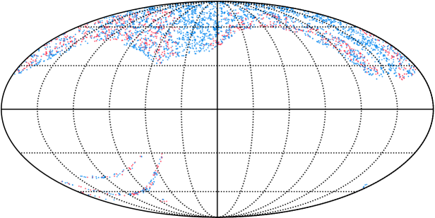
Figure 1: HEALPix projected map of 3512 clusters selected for our analysis, with 908 clusters with BCG spectroscopic redshift in red circles and 2604 clusters with photometric redshift in blue circles. The size of the circles are scaled with $\log_{10}(M_{200})$

The mean and median mass of our cluster sample (including both datasets) are $M^{\mathrm{mean}}_{200}=7.18\times 10^{13}M_{\odot}$ and $M^{\mathrm{median}}_{200}=7.31\times 10^{13}M_{\odot}$, while the mean and median redshift are $z^{\mathrm{mean}}=z^{\mathrm{median}}=0.257$. This results in a mean and a median apparent size of $\theta^{\mathrm{mean}}_{\mathrm{eff}}=\theta^{\mathrm{median}}_{\mathrm{eff}}=3.9^{\prime}$. The full histograms of redshift and apparent angular size for both sets of clusters are shown in the left and right panels of Fig. 2, respectively. The apparent size distributions shown in right panel of Fig. 2 are rather concentrated; their standard deviations are $\sim 0.25$ arcmin. This actually implies that the AAP filter would not yield significant improvement, as compared to the traditional AP filter, for both sets of cluster considered here. We nevertheless adopt the former for the individual-scale measurements, as already noted in Sec. 2.1.2, since it offers a more physical interpretation of the variation of the signal with scale. For the combined measurements in Sec. 3.2, Sec. 4.2, and Sec. 5.2, we adopt the latter as it simplifies the amount of computation involved.

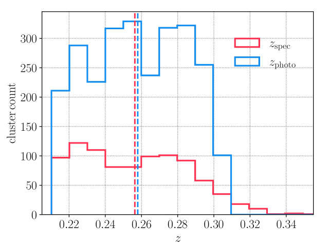
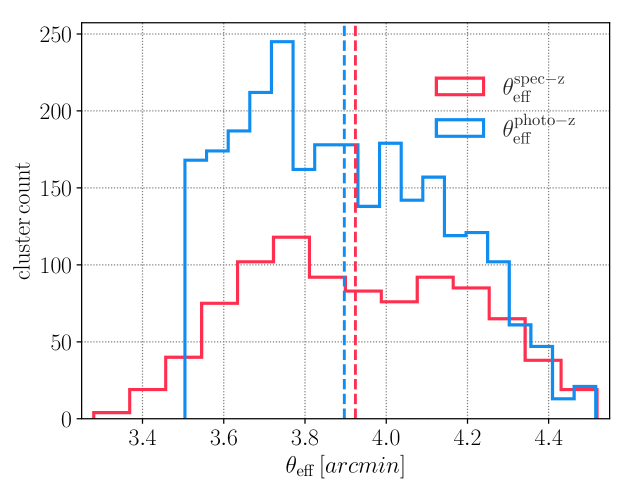
Figure 2: Redshift (left) and apparent size (right) distributions of 3512 maxBCG clusters selected for our analysis. The vertical lines present the mean of redshift distributions for spec-z and photo-z set, respectively.

2.2.2 Modeling maxBCG cluster optical depth

Eq. (1.3) is written for a point source. If a cluster is resolved, we need to integrate Eq. (1.3) over the angular extent $\theta_{\mathrm{eff},i}$ of the cluster. For example, assuming a spherically symmetric Gaussian profile for the electron gas, Eq. (1.3) becomes

$$\tau(\theta_{i},\theta)=\frac{\tau_{0,i}}{\sqrt{2\pi\theta_{\mathrm{eff},i}^{2}}}\int_{0}^{\theta}\textrm{d}^{2}\theta\;\exp\left(-\frac{\left(\theta-\theta_{i}\right)^{2}}{2\,\theta_{\mathrm{eff},i}^{2}}\right),$$ (2.6)

where $\tau_{0,i}$ is the integrated optical depth specific for cluster $i$. We will return to this point below in the discussion following Eq. (3.1).

As the fraction of electrons held by the neutral gas is presumably small, we will assume that all baryons in all the clusters being considered here are fully ionized, i.e. setting $f_{\mathrm{free}}=1$ in $N_{e}=f_{\mathrm{free}}f_{\mathrm{gas}}M_{200,i}/\mu_{e}m_{p}$. We further adopt a universal gas-mass fraction $f_{\mathrm{gas}}=f_{b}\equiv\Omega_{b}/\Omega_{m}=0.16$ following the cosmological baryon abundance and a mean particle weight per electron $\mu_{e}=1.17$. Our expression for the integrated cluster optical depth defined in Eq. (2.6) then becomes

$$\tau_{0,i}=\frac{\sigma_{T}}{D^{2}_{A,i}}\frac{f_{b}M_{200,i}}{\mu_{e}m_{p}}.$$ (2.7)

2.3 borg-SDSS3 reconstructed velocity field

Below, we briefly summarize how the velocity field employed in our analysis is obtained through the process of Bayesian forward modeling, highlighting key features of the borg algorithm and its output. We then detail how we model the large-scale bulk flow of maxBCG clusters using the reconstructed velocity field based on borg-SDSS3 outputs.

2.3.1 borg-SDSS3 reconstruction

We employ the non-linear velocity field set by initial conditions within the SDSS3-BOSS survey volume. The latter is constrained in [38] using the Bayesian forward-modeling algorithm borg [34]. Taking the LOWZ and CMASS galaxies from the SDSS3-BOSS DR13 release [46, 47] as input, borg systematically explores a $256^{3}$-dimensional parameter space of the three-dimensional initial conditions – augmented by the galaxy bias parameters. The algorithm does this essentially by following these three steps repeatedly:

1. Forward-evolving each realization of a Gaussian initial matter field from $z_{\mathrm{ini}}\sim 1000$ to $z=0$. The amplitude of the initial fluctuations is set by the fixed, pre-chosen set of cosmological parameters. In [38], the gravitational forward model used to evolve the initial fluctuations is the first-order Lagrangian perturbation theory [48, 49].

2. Apply a galaxy bias transformation, together with other observational effects, including redshift-space distortion, light-cone effect, survey selection function, foreground contamination, etc. (see Section 2.2-2.6 of [38] for further details), on the evolved matter density field to achieve a predicted galaxy field.

3. Compare the predicted and observed galaxy field (here LOWZ and CMASS) to simultaneously constrain the initial and evolved matter density fields.

The result is a fully probabilistic inference of the cosmic matter and velocity fields, taking into account known and unknown systematic effects (within some pre-defined limits [38]). The setup of the inference is given as follows. The initial conditions are generated on a comoving grid consisting of $256^{3}$ cells and covering a comoving volume of $4000^{3}\,h^{-3}\;\mathrm{Mpc}^{3}$, which corresponds to a grid resolution of $L_{\mathrm{grid}}=15.624\,h^{-1}\;{\rm Mpc}$. The SDSS3-BOSS data are projected in a sub-volume with the observer located at $\bm{x}=\{200,0,-1700\}\,h^{-1}\;{\rm Mpc}$ with respect to the center. A total number of 10360 MCMC samples was collected [38]. Initial power-spectrum analysis in [38] showed that the MCMC chain converged after $\sim 2000$ samples, i.e. the chain has passed its burn-in phase and reached a stationary distribution after the first $\sim 2000$ samples. Here, we consistently remove all samples whose identifier is less than $s=2000$. To facilitate the storage and processing of these samples, the chain is thinned by a factor of 10, i.e. we only include 1-in-every-10 samples in our analysis; more details can be found in [38].

Taking initial conditions constrained by the borg-SDSS3 reconstruction [38] as input, we run DM-only simulations with the same cosmological parameters adopted by the reconstruction using the temporal COmoving Lagrangian Acceleration algorithm [50] (tcola hereafter), and the cloud-in-cell (CIC) projection of particles, to obtain the large-scale velocity field at the maxBCG catalog mean redshift $z=0.23$. This includes in total 837 tcola simulations, one for each of our constrained initial conditions, at the resolution of $N_{\mathrm{part}}=1024^{3}$. These are used for the estimation of cluster LOS velocities as well as their uncertainties.

We additionally generate a GADGET-2 [51] simulation at resolution of $N_{\mathrm{part}}=2048^{3}$ from initial conditions specified by the sample $s=9000$ of borg-SDSS3 reconstruction (see App. D for details). We use this full N-body, high resolution simulation to specifically:

1. estimate the small-scale motion of clusters unresolved by the borg-SDSS3 reconstruction and tcola re-simulation (see Sec. 2.3.2),

2. verify that our kSZ estimators are unbiased (see Sec. 3.1),

3. measure the cluster signal profile (see Sec. 3.2).

2.3.2 Modeling the large-scale bulk flows of galaxy clusters

We model the large-scale bulk flow of galaxy clusters in Eq. (1.2) as a sum of two components:

$$v^{\mathrm{LOS}}(\bm{x},\hat{\bm{n}})=v^{\mathrm{LOS}}_{L}(\bm{x},\hat{\bm{n}})+\epsilon^{\mathrm{LOS}}_{S}(\bm{x},\hat{\bm{n}})\,,$$ (2.8)

where $v^{\mathrm{LOS}}_{L}$ is the large-scale LOS bulk-flow estimated from the borg-SDSS3 reconstruction posterior while $\epsilon^{\mathrm{LOS}}_{S}$ is the unresolved small-scale LOS velocity. We further assume that, for all clusters:

$$\epsilon^{\mathrm{LOS}}_{S}\sim\mathcal{N}\left(0,\sigma_{\epsilon^{\mathrm{LOS}}_{S}}\right)\,,$$ (2.9)

where $\sigma_{\epsilon^{\mathrm{LOS}}_{S}}\simeq 206.12\,\mathrm{km}\mathrm{s}^{-1}$ is estimated from the standard deviation of $\left(v^{\mathrm{LOS}}_{\textsc{nbody},i}-v^{\mathrm{LOS}}_{{t\textsc{cola}},i}\right)$ distribution (see Fig. 3) in which $v^{\mathrm{LOS}}_{\textsc{nbody},i}$ and $v^{\mathrm{LOS}}_{{t\textsc{cola}},i}$ refer to the LOS velocity of halo $i$ as respectively measured from the previously mentioned GADGET-2 simulation and from tcola simulation of the same borg-SDSS3 sample, $s=9000$.

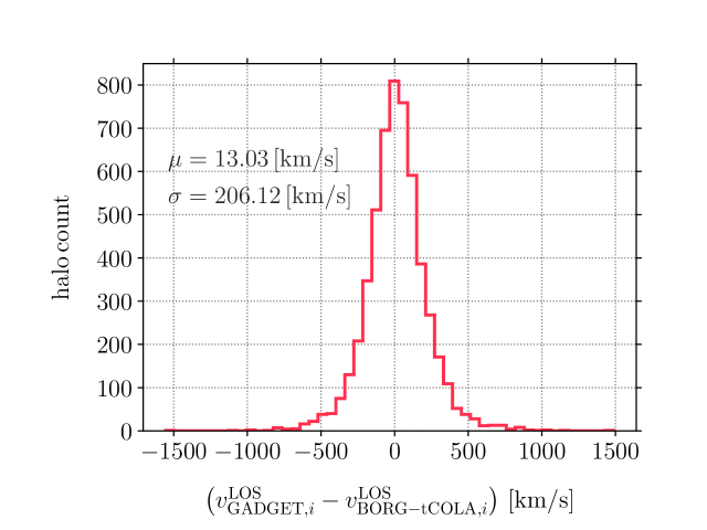
Figure 3: Histogram of $\left(v^{\mathrm{LOS}}_{\textsc{nbody},i}-v^{\mathrm{LOS}}_{{t\textsc{cola}},i}\right)$ measured from DM halos within LOWZ-CMASS volume in our GADGET-2 and tcola simulations of the borg-SDSS3 sample $s=9000$. We apply the same redshift and mass cuts that are applied for maxBCG clusters. The vertical line represents the sample mean. The sample variance is measured at $\sigma^{2}=4.67\times 10^{4}\,\mathrm{km}^{2}\mathrm{s}^{-2}$.

3 Data model and kSZ posterior

Given an inferred ensemble of the large-scale LOS velocity of each galaxy cluster $i$, $v^{\mathrm{LOS}}_{L,i}$, our goal is to construct a likelihood for the extracted kSZ signals at locations of all galaxy clusters in our sample. Below, we will derive this likelihood in two cases of input data:

1. The single-cluster signal is extracted at individual physical scales. This yields multiple measurements of the signal, each using information from a specific scale.

2. The single-cluster signal is simultaneously extracted at multiple scales. This yields one single measurement of the signal combining information from all scales.

While the former can be applied for an analysis focusing on the study of cluster gas profile, we expect the latter to be a more sensitive measurement, as information from all scales is combined and the impact of CMB noise on large scales can be reduced. Our derivations assume that the kSZ measurements at individual cluster locations are independent, i.e. there is no significant overlap between the AP/AAP filters. We verified this is indeed the case for our cluster sample selected from the maxBCG catalog (see Sec. 2.2.1).

3.1 kSZ likelihood: single angular scale

Let us express our data model as

$$\Delta T_{\mathrm{kSZ},i}^{\theta_{f}}/T_{0}=-\alpha^{\theta_{f}}\,\tau_{i}\,v^{\mathrm{LOS}}_{L,i}/c-\tau_{i}\,\epsilon^{\mathrm{LOS}}_{S,\it i}/c+\epsilon^{\theta_{f}}_{0,i}\,,$$ (3.1)

where we have introduced $\alpha^{\theta_{f}}$ as the amplitude of the kSZ signal from the large-scale bulk flow of cluster $i$. Here and below, we simply adopt $\tau_{i}=\tau_{0,i}$. For cases where the filter size is smaller than that of the cluster, this means letting $\alpha^{\theta_{f}}$ absorb all specific details about the cluster gas profile.

We expect to measure a value of $\alpha^{\theta_{f}}$ consistent with zero in the case of no detection, whereas a value of order of unity at filter sizes that are large enough to encompass the whole cluster, i.e. $\theta_{f}\geq\sqrt{\theta^{2}_{\mathrm{vir}}+\theta^{2}_{\mathrm{beam}}}$, corresponds to the expectation from the simple model of optical depth discussed in Sec. 2.2.2. The exact value of $\alpha$ depends on that of $f_{\mathrm{free}}$ (cf. Eq. (2.7)) and on the amount of ionized gas outside but associated with the cluster. Further, it is also sensitive to systematics in the amplitude of the reconstructed velocity field and in the weak lensing mass calibration of galaxy clusters [42]. Hence a direct interpretation of $\alpha$ as $f_{\mathrm{gas}}$ would require careful modeling of these uncertainties. In this paper, we focus on the significance of the kSZ signal detection, which is fortunately not significantly affected by any of those.

In Eq. (3.1), the first noise term on the r.h.s is induced by unresolved small-scale LOS velocity $\epsilon^{\mathrm{LOS},s}_{S,\it i}$ (see Sec. 2.3.2). Note that this term scales with cluster optical depth $\tau_{i}$. It is thus typically negligible for the clusters considered in our analysis. The second noise term $\epsilon^{\theta_{f}}_{0,i}$ denotes the residual of primary CMB anisotropies plus inhomogeneous instrumental noise, which we assume to be a Gaussian random noise with zero mean and variance $\left(\sigma^{\theta_{f}}_{0,i}\right)^{2}$.

Eq. (3.1) holds so long as the tSZ plus other foreground contaminations cancel out. A significant degree of cancelation is expected since they are, to first order, uncorrelated with the LOS large-scale velocity $v^{\mathrm{LOS}}_{L,i}$. Given the cluster mass cut introduced in Sec. 2.2.1, we confirmed that this condition holds (see App. A).

Both the signal amplitude and noise are functions of the AP filter size $\theta_{f}$ (or AAP filter scale $\varphi_{f}$) – as indicated by the superscript $\theta_{f}$. However, for the sake of readability, we will omit the superscript $\theta_{f}$ in all following equations.

The corresponding likelihood distribution for a single velocity realization – as inferred by a borg-SDSS3 sample $s$ – is given by

$$\mathcal{P}\left(\{\Delta T_{\mathrm{kSZ},i}/T_{0}\}\Big{|}\alpha,\,\{\tau_{i}v^{\mathrm{LOS},s}_{L,\it i}/c\}\right)=\\ \prod_{i}\frac{1}{\sqrt{2\,\pi\,\sigma_{i}^{2}}}\exp\left\{-\frac{1}{2\sigma^{2}_{i}}\,\left(\frac{\Delta T_{\mathrm{kSZ},i}}{T_{0}}+\alpha\,\tau_{i}\,\frac{v^{\mathrm{LOS},s}_{L,i}}{c}\right)^{2}\right\}$$ (3.2)

where

$$\sigma^{2}_{i}\equiv\sigma^{2}_{0,i}+(\tau_{i}/c)^{2}\sigma^{2}_{\epsilon^{\mathrm{LOS}}_{S}}.$$ (3.3)

We now seek to construct a posterior distribution for $\alpha$, marginalized over $N$ velocity realizations, i.e.

$$\mathcal{P}\left(\alpha\Big{|}\{\Delta T_{\mathrm{kSZ},i}/T_{0}\}\right) =\int\mathrm{d}\{x_{i}\}\,\mathcal{P}\left(\alpha,\,\{x_{i}\}\Big{|}\Delta T_{\mathrm{kSZ},i}/T_{0}\right)$$ (3.4)

$$\propto\mathcal{P}\left(\alpha\right)\,\int\mathrm{d}\{x_{i}\}\,\mathcal{P}\left(\{x_{i}\}\right)\mathcal{P}\left(\Delta T_{\mathrm{kSZ},i}/T_{0}\Big{|}\alpha,\,\{x_{i}\}\right)\,,$$

where we have used $\{x_{i}\}\equiv\{\tau_{i}\,v_{\mathrm{LOS},i}/c\}$ and introduced the prior on $\alpha$ explicitly as $\mathcal{P}(\alpha)$. The borg-SDSS3 reconstruction provides a sampled approximation

$$\mathcal{P}\left(\{x_{i}\}\right)\approx\frac{1}{N}\sum_{s=1}^{N}\delta^{D}\left(\{x_{i}\}-\{x_{i}\}^{s}\right)\,,$$ (3.5)

where $\delta^{D}(\{x_{i}\})$ denotes the Dirac delta distribution. We thus can rewrite Eq. (3.4) as

$$\mathcal{P}\left(\alpha\Big{|}\{\Delta T_{\mathrm{kSZ},i}/T_{0}\}\right) \propto\mathcal{P}\left(\alpha\right)\frac{1}{N}\sum_{s=1}^{N}\prod_{i}\frac{1}{\sqrt{2\,\pi\,\sigma_{i}^{2}}}\exp\left\{-\frac{1}{2\sigma^{2}_{i}}\,\left(\frac{\Delta T_{\mathrm{kSZ},i}}{T_{0}}+\alpha\,x^{s}_{i}\right)^{2}\right\}\,,$$ (3.6)

$$\propto\mathcal{P}\left(\alpha\right)\sum_{s}^{N}\lambda_{s}\frac{\exp\left(-\,\frac{\left(\alpha-\mu_{s}\right)^{2}}{\,2\left(\sigma_{s}\right)^{2}}\right)}{\sqrt{2\pi\,\left(\sigma_{s}\right)^{2}}}\,,$$ (3.7)

which is a mixture of Gaussian distributions. Each component of the mixture consists of an individual velocity realization – indexed by $s$ – associated with a mixture weight $\lambda_{s}$, which is given by (see App. B for a detailed derivation)

$$\lambda_{s}=\frac{\exp\left[\omega_{s}\,+\frac{1}{2}\mathrm{ln}(2\pi\,\left(\sigma_{s}\right)^{2})\right]}{\sum_{s}^{N}\exp\left[\omega_{s}\,+\frac{1}{2}\mathrm{ln}(2\pi\,\left(\sigma_{s}\right)^{2})\right]},$$ (3.8)

in which

$$\sigma_{s}^{2}=\left[\sum_{i}\left(\frac{x^{s}_{i}}{\sigma_{i}}\right)^{2}\right]^{-1},$$ (3.9)

and

$$\omega_{s}\equiv\mu^{2}_{s}/\left(2\sigma^{2}_{s}\right),\,\,\,\,\mu_{s}=\frac{\sum_{i}\left[\left(\Delta T_{\mathrm{kSZ},i}/T_{0}\right)\,x^{s}_{i}\right]/\sigma_{i}^{2}}{\sum_{i}\left(x^{s}_{i}/\sigma_{i}\right)^{2}}.$$ (3.10)

Note that the weights $\lambda_{s}$ give preference to better-fitting realizations of the peculiar velocity field, and $\sum_{s}^{N}\lambda_{s}=1$.

For simplicity, in what follows, we assume a uniform prior on $\alpha$ such that $\mathcal{P}(\alpha)=1$ for all borg-SDSS3 velocity realizations. The posterior mean estimate of $\alpha$ is then given by (see App. B for details)

$$\langle\alpha\rangle_{s}=\sum_{s}^{N}\lambda_{s}\mu_{s}=\sum_{s}^{N}\lambda_{s}\,\frac{\sum_{i}\left[\left(\Delta T_{\mathrm{kSZ},i}/T_{0}\right)\,x^{s}_{i}\right]/\sigma_{i}^{2}}{\sum_{i}\left(x^{s}_{i}/\sigma_{i}\right)^{2}},$$ (3.11)

while its variance is given by

$$\sigma^{2}_{\alpha}=\sum_{s}^{N}\lambda_{s}\sigma_{s}^{2}+\sum_{s}^{N}\lambda_{s}\,\left(\mu_{s}-\langle\alpha\rangle_{s}\right)^{2}.$$ (3.12)

In the Bayesian language, the significance of each kSZ measurement in supporting the positive-kSZ hypothesis (against the no-kSZ hypothesis) would be quantified through the Bayes factor. In our particular case, this factor can be directly computed as the ratio between two cumulative distribution functions (CDF) of positive-kSZ $\mathcal{P}(\alpha>0)$ and no-kSZ hypothesis $\mathcal{P}(\alpha\leq 0)$:

$$BF=\frac{\mathcal{P}\left(\alpha>0\Big{|}\{\Delta T_{\mathrm{kSZ},i}/T_{0}\}\right)}{\mathcal{P}\left(\alpha\leq 0\Big{|}\{\Delta T_{\mathrm{kSZ},i}/T_{0}\}\right)}.$$ (3.13)

Previous kSZ measurements in literature, however, usually reported their significance in terms of distance between the measurement and the value of the null hypothesis, measured in multiples of standard deviation $\sigma$ of a normal distribution [see, e.g. 6, 12, 29, 13, 30]. To facilitate a direct comparison, we adopt the same unit by matching the CDF of the normal distribution to that of our posterior distribution, i.e.

$$\mathcal{P}_{\mathrm{normal}}\left(x\leq-\mathrm{sign.}\right)=\mathcal{P}(\alpha\leq 0)\,,$$ (3.14)

and sign. would be our significance measured in the familiar unit of $\sigma$.

Note that Eq. (3.11) is identical to Eq. (9) in [29] if one takes all $\lambda_{s}=1$ and neglects the uncertainty in the velocity reconstruction process. As can be seen in Eq. (3.12), our estimator properly includes systematic uncertainties in this step. To better illustrate this point, in Fig. 4, we compare the uncertainty on the inferred amplitude when one only has a single velocity realization $s$, and when one has an ensemble of realizations $\{s\}$. The single realization case consistently underestimates the uncertainty by – from small to large scales – $\simeq 10-20\%$. It is worth pointing out also that different realizations yield different estimates of $\alpha_{s}$ itself. A combination of, say, high $\alpha_{s}$ and low $\sigma_{\alpha_{s}}$, can significantly bias the significance of any kSZ detection that does not account for uncertainties in velocity reconstruction. We note that this trend might explain the large variation in detection significance of previous kSZ measurements, as, for example, summarized in Tab. 1 of [52]. In our case, the significance can be biased by as high as a factor of 2 if one cherry-picks only one single best-fitting borg-SDSS3 velocity realization.

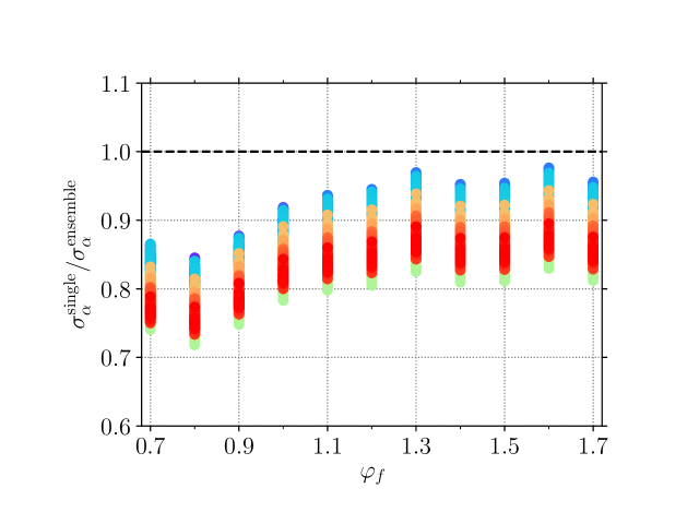
Figure 4: Ratio between the uncertainty on $\langle\alpha\rangle_{s}$ when having only one single realization of the peculiar velocity field, as in the cases reported so far in the literature, and that when having instead an ensemble of realizations, as in our case. Each color point represents a realization of the reconstructed velocity field, corresponding to a borg-SDSS3 MCMC sample.

We further test our estimator in Eq. (3.11) on mock input data where a kSZ signal template – generated by DM halos in the GADGET-2 simulation of the borg-SDSS3 sample $s=9000$ (see App. D), assuming a Gaussian gas profile – is injected into a SMICA2018-like CMB map (including both primary CMB and instrumental noise). By artificially varying the noise level, we verified that our estimator is indeed unbiased. In the limit of vanishing noise, we obtain $\lambda_{s=9000}\to 1$ while the other weights go to zero, correctly singling out the original borg-SDSS3 sample used to generate the mock signal template.

3.2 kSZ likelihood: combined signal

To combine measurements at different filter sizes $\theta_{f}$, it is necessary to modify Eqs. (3.1)–(3.7) to include the cluster gas profile $f(\theta_{f})$ as

$$\tau_{i}=\tau_{i,0}\,f^{\theta_{f}},$$ (3.15)

where we have assumed that this profile is universal. In this work, we obtain an estimate this profile by applying our pipeline on a pure-kSZ signal template generated from individual DM particles found in the GADGET-2 high-resolution simulation (see details in App. D). We show below, in Fig. 5, the measurement of $f^{\theta_{f}}$ at locations of corresponding DM halos identified by Rockstar halo finder [53, 54], an adaptive hierarchical friends-of-friends (FoF) algorithm in six-dimensional phase-space. Note that we use the same velocity field to assign LOS velocity to the DM particles and halos. For simplicity, in case of the combined signal, we restrict ourselves to the AP filter whose $\theta_{f}$ does not depend on the cluster effective apparent size.

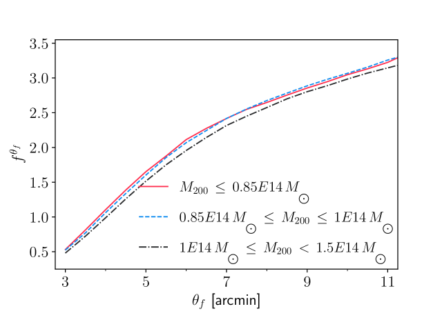
Figure 5: The profile $f^{\theta_{f}}$ at locations of DM halos measured from our mock kSZ template generated by member particles in the GADGET-2 simulation detailed in App. D. As a consistency check, we divide our DM halo sample of $M_{200}\leq 1.5\times 10^{14}M_{\odot}$ into three mass bins as shown in the plot. Below $M_{200}\leq 10^{14}M_{\odot}$, the profile is not very sensitive to $M_{200}$. Only the result for $M_{200}\leq 0.85\times 10^{14}M_{\odot}$ is used in our analysis.

Eq. (3.1) now becomes

$$\overrightarrow{\Delta T}_{\mathrm{kSZ},i}/T_{0}=-\alpha\,\tau_{i,0}\vec{f}\,\left(v^{\mathrm{LOS}}_{L,i}/c\right)-\tau_{i,0}\vec{f}\,\left(\epsilon^{\mathrm{LOS},s}_{S,\it i}/c\right)+\vec{\epsilon}_{0,i}\,,$$ (3.16)

where we have again omitted the superscript $\theta_{f}$ and instead expressed quantities that depend on $\theta_{f}$ as vectors to stress the fact that all measurements at different filter scales are now combined in Eq. (3.16). Note also that $\alpha$ is now simply a scalar instead of a function of $\theta_{f}$. Eq. (3.2) can then be rewritten as

$$\mathcal{P}\left(\{\overrightarrow{\Delta T}_{\mathrm{kSZ},i}/T_{0}\}|\alpha,\,\tau_{i,0}\vec{f}\left(v^{\mathrm{LOS},s}_{L,i}/c\right)\}\right)\propto\prod_{i}|\mathbf{C}_{i}|^{-1/2}\\ \quad\times\>\,\exp\left\{-\frac{1}{2}\,\left[\overrightarrow{\Delta T}_{\mathrm{kSZ},i}/T_{0}+\alpha\,\tau_{i,0}\vec{f}\,\left(v^{\mathrm{LOS},s}_{L,i}/c\right)\right]^{\intercal}\,\left(\mathbf{C}_{i}\right)^{-1}\,\left[\overrightarrow{\Delta T}_{\mathrm{kSZ},i}/T_{0}+\alpha\,\tau_{i,0}\vec{f}\,\left(v^{\mathrm{LOS},s}_{L,i}/c\right)\right]\right\}$$ (3.17)

where the covariance matrix $\mathbf{C}_{i}$ for cluster $i$ is given by

$$C^{\theta_{f}\theta_{f}^{\prime}}_{i}=\left\langle\frac{\Delta T^{\theta_{f}}_{\mathrm{CMB}}(\bm{\theta_{i}})}{T_{0}}\frac{\Delta T^{\theta_{f}^{\prime}}_{\mathrm{CMB}}(\bm{\theta_{i}})}{T_{0}}\right\rangle\,+\left\langle\frac{\Delta T^{\theta_{f}}_{\mathrm{instr}}(\bm{\theta_{i}})}{T_{0}}\frac{\Delta T^{\theta_{f}^{\prime}}_{\mathrm{instr}}(\bm{\theta_{i}})}{T_{0}}\right\rangle\,+\,\tau^{2}_{i,0}f^{\theta_{f}}f^{\theta_{f}^{\prime}}\sigma^{2}_{\epsilon^{\mathrm{LOS}}_{S}}\,,$$ (3.18)

in which we have separated the primary CMB anisotropy and the instrumental noise into the first and second term, respectively. Although, for completeness, we do include the last term on the r.h.s. of Eq. (3.18) in our covariance estimate, we note that it is negligible compared to the first two terms – as it scales with $\tau^{2}$ – and the exclusion of this term would affect neither the signal amplitude nor significance. The second noise contribution is highly inhomogeneous due to the scanning strategy of the Planck satellite and requires instrument-specific mocks to estimate [55, 56]. To this end, it is worth mentioning that Planck does provide a limited set of 300 noise and residual systematics simulations for SMICA2018 [36]. For this work, we instead choose to generate 2500 instrumental noise maps in which the noise value of each pixel is drawn from a zero-mean Gaussian whose variance is given by the corresponding temperature intensity variance in the Planck 2018 HFI Sky Map at frequency 143GHz [56, 55] (see details in App. C). While this estimate is likely conservative since SMICA is a weighted linear combination of multiple frequency channels, we expect it to be robust and stable, especially at small filter sizes where this term dominates. The first term could be estimated analytically using the Planck 2018 best-fit $\Lambda$CDM power spectrum [57]. In the flat-sky limit,

$$\Delta T_{\mathrm{CMB}}^{\theta_{f}}(\bm{\theta_{i}})=\int\frac{d\bm{\ell}}{(2\pi)^{2}}\,\exp{\left(i\bm{\ell}\cdot\bm{\theta_{i}}\right)}\,(\pi\theta_{f}^{2})\,W(\ell\theta_{f})\,\Delta T_{\mathrm{CMB}}^{{\mathrm{obs}}}(\bm{\ell}),$$ (3.19)

where $W(l\theta_{f})$ is the Fourier transform of the AP filter

$$W\left(\ell\theta_{f}\right)=2\,\left[W_{\rm TH}\left(\ell\theta_{f}\right)\,-\,W_{\rm TH}\left(\sqrt{2}\ell\theta_{f}\right)\right],\qquad W_{\rm TH}\left(\ell\theta_{f}\right)=2\frac{J_{1}\left(\ell\theta_{f}\right)}{\ell\theta_{f}},$$ (3.20)

while $\bm{\ell}$ is the two-dimensional wavevector perpendicular to the LOS, $\ell=|\bm{\ell}|$, and

$$\Delta T_{\mathrm{CMB}}^{{\mathrm{obs}}}(\bm{\ell})=\Delta T_{\mathrm{CMB}}(\bm{\ell})B(\bm{\ell}).$$ (3.21)

The CMB covariance matrix in Eq. (3.18) is then explicitly given by (see App. C)

$$\mathbf{C}^{\theta_{f}\theta_{f}^{\prime}}_{\mathrm{CMB},i}=\frac{\pi\theta_{f}^{2}(\theta^{\prime}_{f})^{2}}{2T_{0}^{2}}\,\int_{0}^{\infty}d\ell\,\ell\,W\left(\ell\theta_{f}\right)\,W\left(\ell\theta_{f}^{\prime}\right)\,C^{\mathrm{CMB}}_{\ell},$$ (3.22)

where $C^{\mathrm{CMB}}_{\ell}$ denotes the Planck 2018 $\Lambda$CDM best fit angular power spectrum. We show in Fig. 6 the CMB correlation matrix evaluated from Eq. (3.22), the instrumental noise correlation matrix estimated, for one single cluster, from 2500 instrumental noise mocks, and the corresponding total correlation matrix of the AP measurements (including both primary CMB and instrumental noise contributions) at different filter sizes estimated by Eq. (3.18). Note that the last two vary between cluster locations due to the inhomogeneity of the Planck instrumental noise.

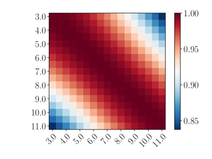
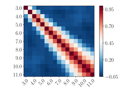
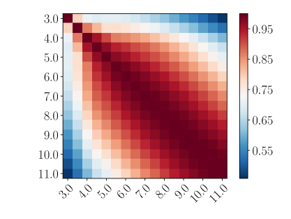
Figure 6: Top: Correlation matrices of the primary CMB (left panel) and instrumental noise (right panel), as described by the first and second term on the r.h.s. of Eq. (3.18). Bottom: The total noise correlation matrix, evaluated using the full r.h.s. of Eq. (3.18).

We use the covariance matrix estimated by Eq. (3.18) for both the individual-scale and combined measurements of the signal. Specifically, for the individual-scale case which employs the AAP filter, we interpolate $\sigma^{2}_{\mathrm{CMB},i}$ (cf. Eq. (3.3)) from a 1024x1024 $\mathbf{C}^{\theta_{f}\theta_{f}^{\prime}}_{\mathrm{CMB}}$ matrix.

The posterior of $\alpha$ given measurements at all filter sizes can be constructed similarly to Eq. (3.7)

$$\mathcal{P}\left(\alpha|\{\overrightarrow{\Delta T}_{\mathrm{kSZ},i}/T_{0}\}\right) \propto\mathcal{P}\left(\alpha\right)\frac{1}{N}\sum_{s=1}^{N}\prod_{i}|\vec{C}_{i}|^{-1/2}$$ (3.23)

$$\exp\left\{-\frac{1}{2}\,\left[\overrightarrow{\Delta T}_{\mathrm{kSZ},i}/T_{0}+\alpha\,\vec{x}^{s}_{i}\right]^{\intercal}\,\left(\vec{C}_{i}\right)^{-1}\,\left[\overrightarrow{\Delta T}_{\mathrm{kSZ},i}/T_{0}+\alpha\,\vec{x}^{s}\right]\right\}$$

where we have similarly used $\vec{x}^{s}_{i}\equiv\left\{\tau_{i,0}\vec{f}\,\left(v^{\mathrm{LOS},s}_{L,i}/c\right)\right\}$.

The expressions of the posterior mean $\langle\alpha\rangle_{n}$ and its variance $\sigma^{2}_{\alpha}$ are similar to those in Eq. (3.11) and Eq. (3.12) with modifications to $\mu_{s}$ and $\omega_{s}$ as described in App. B.

3.3 Modeling photo-z uncertainty

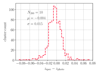
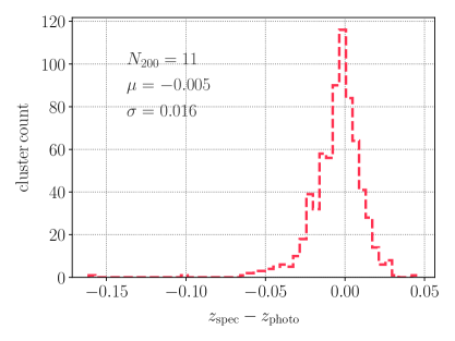
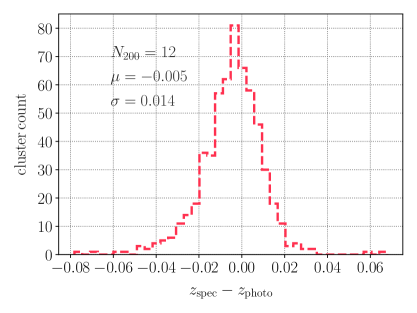
Figure 7: Histograms of differences between BCG spectroscopic redshift and cluster photometric redshift for 2129 maxBCG clusters below $M_{200}=0.85\times 10^{14}M_{\odot}$. We separate the clusters into three bins of richness $N_{200}=10$ (top, left panel), $N_{200}=11$ (top, right panel), $N_{200}=12$ (bottom panel) but detect no dependence of photo-z error on cluster richness. For clarity, the mean $\mu$ and standard deviation $\sigma$ of each histogram are additionally shown.

To account for uncertainties in $v^{\mathrm{LOS},s}_{L,i}$ induced by photometric redshift error (see left panel of Fig. 7), we introduce an additional sampling step. Specifically, we generate a sample of $N_{r}$ realizations of maxBCG cluster positions in redshift space, in which we keep the redshifts of spec-z clusters fixed while sampling those of photo-z clusters as

$$z^{r}_{\mathrm{photo},i}=z^{0}_{\mathrm{photo},i}+\delta z^{r}_{i}\,,$$ (3.24)

wherein $z^{0}_{\mathrm{photo},i}$ is the fiducial photometric redshift of cluster $i$ and

$$\delta z^{r}_{i}\sim\mathcal{N}\left(0,\sigma_{z}\right).$$ (3.25)

Here, $\mathcal{N}\left(0,\sigma_{z}\right)$ is a zero-mean Gaussian with a standard deviation of $\sigma_{z}=0.015$. The latter value follows the scatter between spectroscopic and photometric redshifts of reference clusters $\sigma_{z}=\langle\sigma[z_{\mathrm{spec}}(N_{200})-z_{\mathrm{photo}}(N_{200})]\rangle$, averaged over three $N_{200}=[10,11,12]$ bins. As indicated in the right panel of Fig. 7, this scatter shows no strong dependence on richness for the clusters considered in our analysis. Note that we have assumed that there is no bias in the fiducial $z_{\mathrm{photo}}$, as the public version of maxBCG catalog is reportedly corrected for this effect [37]. Additionally, we verified that our results are not significantly affected if we are to correct for a possible small bias of the order $\mu\simeq-0.005$ in $z_{\mathrm{photo}}$ (see Fig. 7).

Note that when drawing from the Gaussian distribution in Eq. (3.25), we limit the range of $z^{r}_{\mathrm{photo},i}$ in all redshift realizations to within $[0.05,0.5]$. So our Gaussian distributions of photometric redshift error are actually truncated.

We then introduce an additional sum over all $N_{r}$ redshift realizations in Eq. (3.7),

$$\mathcal{P}\left(\alpha|\{\Delta T_{\mathrm{kSZ},i}/T_{0}\}\right)=$$ (3.26)

$$\qquad\mathcal{P}\left(\alpha\right)\frac{1}{N_{r}}\sum_{r=1}^{N_{r}}\frac{1}{N_{s}}\sum_{s=1}^{N_{s}}\prod_{i}\frac{1}{\sqrt{2\,\pi\,\sigma_{i}^{2}}}\exp\left\{-\frac{1}{2\sigma_{i}^{2}}\,\left(\frac{\Delta T_{\mathrm{kSZ},i}}{T_{0}}+\alpha\,\tau_{i}v^{\mathrm{LOS},sr}_{L,i}/c\right)^{2}\right\}.$$

Note that, in the case of the AAP filter, for all redshift realizations, we keep the filter size in Eq. (3.26) fixed as $\theta_{f}=\varphi_{f}\,\theta^{0}_{200,i}$ where $\theta^{0}_{200,i}$ is computed from the fiducial values $z^{0}_{\mathrm{photo},i}$. Given the range in which the apparent size of selected maxBCG clusters varies (see right panel of Fig. 2), this approximation does not affect our estimator in any significant way.

Since the two indices $s$ and $r$ in Eq. (3.26) are mathematically equivalent – in the sense that they only appear in $v^{\mathrm{LOS},sr}_{L,i}$ – we can rewrite them as

$$n\equiv\left\{s,\!r\right\}$$ (3.27)

and

$$v^{\mathrm{LOS},\ n}_{L,i}\equiv v^{\mathrm{LOS},s}_{L,i}\left(z^{r}_{\mathrm{photo},i}\right)$$ (3.28)

so that

$$\mathcal{P}\left(\alpha|\{\Delta T_{\mathrm{kSZ},i}/T_{0}\}\right)=\mathcal{P}\left(\alpha\right)\frac{1}{N}\sum_{n=1}^{N}\prod_{i}\frac{1}{\sqrt{2\,\pi\,\sigma_{i}^{2}}}\exp\left\{-\frac{1}{2\sigma_{i}^{2}}\,\left(\frac{\Delta T_{\mathrm{kSZ},i}}{T_{0}}+\alpha\,x^{n}_{i}\right)^{2}\right\}\,,$$ (3.29)

where $N=N_{r}\,N_{s}$ and $x^{n}_{i}\equiv\tau_{i}v^{\mathrm{LOS},n}_{L,i}/c$.

The derivation of the estimator $\left\langle\alpha\right\rangle_{n}$ and its uncertainty $\sigma^{2}_{\alpha}$ is then almost identical to that in Sec. 3 and App. B, only with $s$ replaced by $n$.

4 Results

Below we report the results of our measurement of the kSZ effect, imprinted by selected maxBCG clusters on the SMICA2018 CMB map, in terms of the posterior mean $\langle\alpha^{\varphi_{f}}\rangle_{n}$ – over velocity and redshift realizations (cf. Eq. (3.11)) – and the associated significance (cf. Eq. (3.14)).

4.1 Individual-scale signal measurements

We show in Fig. 8 the inferred value of $\langle\alpha^{\varphi_{f}}\rangle_{n}$ as a function of the AAP filter scale $\varphi_{f}$, using spec-z set alone (top panel) or photo-z set and both sets (bottom panel). We emphasize again that the $1\sigma$ uncertainty shown here as shaded band and reported in Tab. 1 includes also uncertainties in the reconstructed large-scale velocity field.

As can be noted from Fig. 8, we obtain consistent results between the two datasets spec-z and photo-z, which can be combined as shown in red in the bottom panel of Fig. 8. Note that the slightly larger uncertainty region of $\langle\alpha\rangle_{n}$ measurement using spec-z set – compared to that of $\langle\alpha\rangle_{n}$ measurement using photo-z set – is mostly caused by their limited quantity, as suggested by the ratio between the two uncertainties being approximately constant across all filter scales. Both panels of Fig. 8 show that most of the information come from small scales. As the filter scale increases, the AAP estimate picks up more and more contribution from primary CMB anisotropies, as well as other large-scale sources of contamination, and quickly loose its constraining power.

In addition, we provide the significance at each filter scale for each dataset in Tab. 1. All sets show peaks of significance at $\varphi=0.9$, close to the angular cluster scale as one should expect. Further, for the photo-z set, the photo-z uncertainty shows a bigger impact at small filter sizes, which is also an expected behavior, since on large scales, the primary CMB is still the dominant noise source.

For illustration, we additionally show the mixture weights (cf. Eq. (3.8)) in Fig. 9, since it can provide some insights on how the information in spec-z and photo-z sets are combined. One can see that the distributions of $\lambda_{s}$ in the three panels on the right of Fig. 9, which show $\lambda_{s}$ for the combined set, are consistent with those of $\lambda_{s}$ in the leftmost and middle columns, which respectively show $\lambda_{s}$ for spec-z and photo-z set. This implies that Eq. (3.29) consistently combines information from the spec-z and photo-z to simultaneously and correctly pick out the better-fitting borg-SDSS3 samples and redshift realizations.

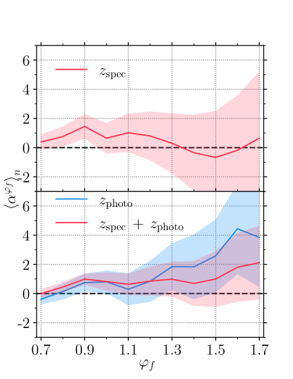
Figure 8: The posterior mean of the kSZ signal amplitude $\left\langle\alpha\right\rangle_{n}$ measured at different AAP filter scales $\varphi_{f}=[0.7,1.6]$ using spec-z (top panel, red) or photo-z (bottom panel, blue) and both sets (bottom panel, red). The shaded regions denote the corresponding $1\,\sigma$ uncertainties, which, in our case, including both uncertainties in CMB anisotropies and the reconstructed velocity field.

$\varphi_{f}$	spec-z		photo-z		spec-z + photo-z
	$\langle\alpha^{\varphi_{f}}\rangle_{n}$	sign.	$\langle\alpha^{\varphi_{f}}\rangle_{n}$	sign.	$\langle\alpha^{\varphi_{f}}\rangle_{n}$	sign.
0.7	$0.38\pm 0.52$	0.76	$-0.39\pm 0.36$	-1.06	$-0.01\pm 0.29$	-0.09
0.8	$0.76\pm 0.68$	1.13	$0.14\pm 0.54$	0.27	$0.44\pm 0.37$	1.16
0.9	$1.45\pm 0.84$	1.71	$0.75\pm 0.61$	1.19	$0.99\pm 0.39$	2.21
1.0	$0.65\pm 1.04$	0.63	$0.80\pm 0.79$	0.98	$0.82\pm 0.62$	1.27
1.1	$1.02\pm 1.32$	0.78	$0.29\pm 1.09$	0.30	$0.63\pm 0.74$	0.85
1.2	$0.80\pm 1.67$	0.48	$0.84\pm 1.41$	0.61	$0.85\pm 0.99$	0.84
1.3	$0.30\pm 2.05$	0.15	$1.84\pm 1.60$	1.09	$0.98\pm 1.19$	0.81
1.4	$-0.35\pm 2.60$	-0.14	$1.83\pm 2.22$	0.85	$0.69\pm 1.53$	0.46
1.5	$-0.67\pm 3.18$	-0.21	$2.58\pm 2.51$	0.99	$0.99\pm 1.92$	0.51
1.6	$-0.18\pm 3.76$	-0.05	$4.44\pm 3.11$	1.32	$1.80\pm 2.36$	0.76
1.7	$0.65\pm 4.58$	0.14	$3.84\pm 3.39$	1.08	$2.12\pm 2.52$	0.83

Table 1: The posterior mean of the kSZ signal amplitude $\langle\alpha\rangle_{n}\pm 1\sigma_{\alpha}$ measured at individual AAP filter scales, and the detection significance (cf. Eq. (3.14)) are shown for, from left to right, spec-z, photo-z and both datasets. The maximum significance in each case is highlighted.

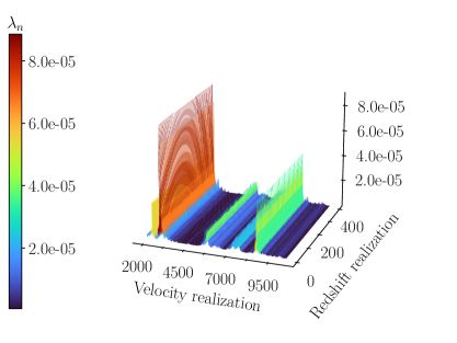
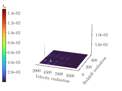
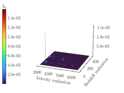
Figure 9: Distributions of the mixture weight $\lambda_{n}$ over 837 borg-SDSS3 velocity realizations with mcmc identifier 2000-10360 (x-axes) and 400 redshift realizations (y-axes) for the cases of spec-z (left), photo-z (middle) and both datasets combined (right) at $\varphi=0.9$. Note that we do not sample the redshifts of clusters in the spec-z set, which is why the $\lambda_{n}$ are evenly distributed among redshift realizations (y-axes) in the leftmost column.

4.2 Combined signal measurement

We show in Fig. 10 our measurements of combined signal amplitude $\langle\alpha^{\theta_{f}}\rangle_{n}$ (cf. Eq. (3.11)), as a cumulative function of the AP filter radius $\theta_{f}$, for spec-z or photo-z set separately and both sets combined.

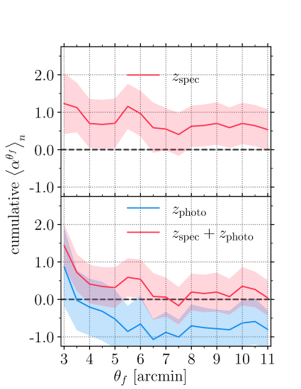
Figure 10: The posterior mean of the kSZ combined signal amplitude $\left\langle\alpha\right\rangle_{n}$ combining measurements at progressively larger AP filter sizes, $\theta_{f}=[3.0,11.0]$ arcmin, using spec-z (top panel, red) or photo-z (bottom panel, blue) and both sets (bottom panel, red). Going from left to right, each data point combines information from all previous points. The shaded regions denote the corresponding $1\,\sigma$ uncertainties, including both uncertainties in CMB anisotropies and the reconstructed velocity field.

As can be seen from both cases of individual- and combined signal, the uncertainty in photometric redshift, when accounted for by double sampling, reduces the constraining power of the photo-z set, i.e. adding the clusters from the photo-z set does not substantially improve our significance. The most physically important factor is whether the photo-z error can be well-approximated by a symmetric distribution, for example, the Gaussian, centered on the fiducial redshift. As clusters are virialized, collapsed objects, they are more likely to form in overdense regions. It is then reasonable to suspect that the photo-z fluctuations are not symmetrically distributed around the inferred value by the maxBCG algorithm, but rather biased towards overdense regions along the respective line of sight. Further detailed investigation is thus required to identify the optimal way to combine information from both spectroscopic and photometric data, subject to current constraints on computational resources. We defer such an investigation to future work.

The significance of the cumulative combined signal for each dataset is summarized in Tab. 2. As in Tab. 1, most of the information is limited to filter sizes below and around the apparent size of maxBCG clusters in our samples. Above that scale, CMB noise severely limits our significance. This suggests that data from current CMB experiments such as ACTpol and SPT-3G with their much higher resolutions, $\sim 1$ arcmin [58, 59], can improve our significance significantly. On the other hand, even at the modest resolution of $\sim 2-3$ arcmin, we expect a future experiment such as CMB-S4, with much lower instrumental noise, to also yield a significantly improved measurement. In both cases, the details of the gas profile would become important and one would almost certainly need to go beyond the Gaussian profile and the AP filter case considered here.

$\theta_{f}$ [arcmin]	spec-z		photo-z		spec-z + photo-z
	$\langle\alpha^{\varphi_{f}}\rangle_{n}$	sign.	$\langle\alpha^{\varphi_{f}}\rangle_{n}$	sign.	$\langle\alpha^{\varphi_{f}}\rangle_{n}$	sign.
3.0	$1.23\pm 0.81$	1.51	$0.87\pm 1.04$	0.81	$1.44\pm 0.57$	2.09
3.5	$1.12\pm 0.66$	1.67	$-0.02\pm 0.80$	-0.01	$0.72\pm 0.49$	1.39
4.0	$0.70\pm 0.65$	1.07	$-0.21\pm 0.76$	-0.26	$0.41\pm 0.51$	0.79
4.5	$0.67\pm 0.66$	1.03	$-0.32\pm 0.78$	-0.40	$0.34\pm 0.51$	0.67
5.0	$0.70\pm 0.66$	1.07	$-0.53\pm 0.78$	-0.66	$0.32\pm 0.54$	0.60
5.5	$1.16\pm 0.60$	1.88	$-0.86\pm 0.68$	-1.15	$0.59\pm 0.51$	1.12
6.0	$0.96\pm 0.61$	1.56	$-0.66\pm 0.75$	-0.90	$0.54\pm 0.53$	0.98
6.5	$0.58\pm 0.67$	0.91	$-1.07\pm 0.55$	-1.63	$0.08\pm 0.62$	0.11
7.0	$0.55\pm 0.56$	0.98	$-0.88\pm 0.55$	-1.41	$0.06\pm 0.52$	0.12

Table 2: The posterior mean of the kSZ combined signal amplitude $\langle\alpha\rangle_{n}\pm 1\sigma_{\alpha}$ measured at increasing maximum AP filter size, and the corresponding detection significance (cf. Eq. (3.14)) are shown for spec-z, photo-z and both datasets (left to right). The maximum significance in each case is highlighted. Note that, for readability we only list here results for $\theta_{f}=[3,7]$ arcmin.

5 Null tests for systematics

In this section, we further assert the significance of our measurement by performing two null tests on mock data in which we

1. shuffle the position of the clusters in our analysis, and

2. replace the SMICA2018 by a set of 300 SMICA-like mock maps, also taken from Planck 2018 data release [36].

Since the photo-z set adds very little information, in the tests below, we will only focus on the spec-z set. We have found that the significance computed from Eq. (3.14) can be rather well approximated by the simple ratio S/N=$\langle\alpha^{\varphi_{f}}\rangle_{n}/\sigma_{\alpha}$. Below, we employ this approximation to ease the numerical computation of the significance in these null tests.

5.1 Null tests: Individual-scale signal

For the case of individual-scale measurements using the AAP filter, we measure a signal amplitude consistent with zero for the spec-z set with cluster positions being shuffled, as can be seen in the left panel of Fig. 11. When applying our pipeline on the set of 300 SMICA2018 simulations (including CMB and instrumental noise) provided by Planck [36], we also recover S/N ratios consistent with zero-mean Gaussian distributions. We show in the top panels of Fig. 12 the histograms of S/N for increasing individual filter scale from $\varphi=0.9$ to $\varphi=1.1$. The histogram of $\varphi=0.9$ (top row, left panel) appears consistent with our reported significances of $\simeq 1.7$ for the spec-z dataset (cf. Tab. 1).

5.2 Null tests: combined signal

For the case of cumulative multi-scale measurements using the AP filter, we also measure a cumulative signal amplitude consistent with zero for spec-z set with cluster positions being shuffled, as shown in Fig. 11. Our null test using the Planck simulations also recovers S/N ratios consistent with zero-mean Gaussian distributions. We show in Fig. 12 the histograms of S/N for cumulative multi-scale from $\theta_{f}=3.0-3.5$ arcmin to $\theta_{f}=3.0-5.5$ arcmin. The histogram of $\theta_{f}=3.0-5.5$ arcmin (bottom row, right panel) again shows that our reported significance of $\simeq 1.9$ for the spec-z set (cf. Tab. 2) is consistent with the 95% confidence interval.

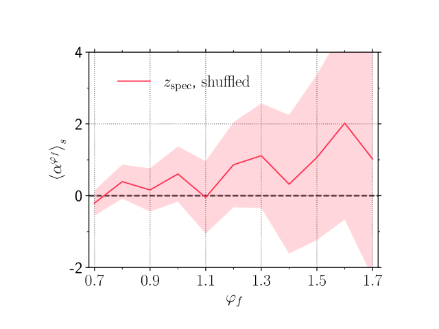
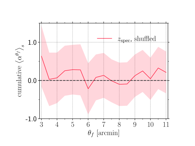
Figure 11: Left panel: Individual-scale signal amplitude measured using spec-z sample but with sky positions of the clusters shuffled, plotted as a function of AAP filter scale. Right panel: combined signal amplitude measured using spec-z set but with sky positions of the clusters shuffled, plotted as a cumulative function of AP filter sizes.

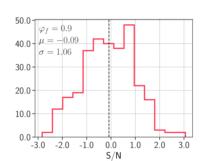
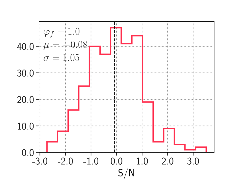
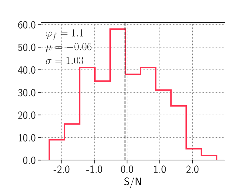
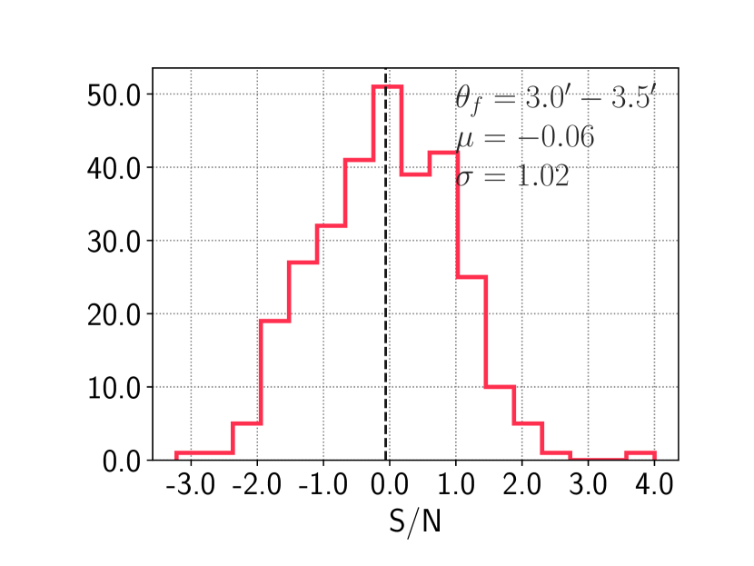
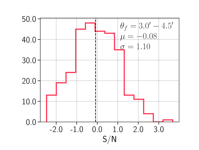
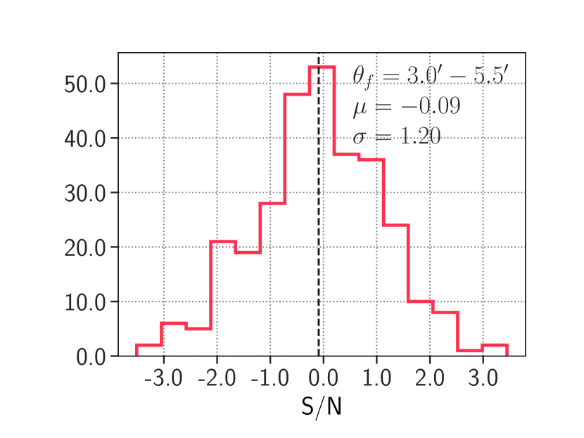
Figure 12: Top: Histograms of the S/N of individual-scale signal for spec-z set, measured at $\varphi_{f}=[0.9,1.0,1.1]$, from 300 simulations of SMICA2018 (including CMB and SMICA-like instrumental noise). The vertical dashed line presents the mean in each histogram. For clarity, the mean $\mu$ and standard deviation $\sigma$ of each histogram are also shown in each plot. Bottom: Histograms of the S/N of multi-scale signal for spec-z set, measured cumulatively between $\theta_{f}=3.0$ and $\theta_{f}=5.5$ arcmin, from 300 simulations of SMICA2018 (including CMB and SMICA-like instrumental noise). The vertical dashed line presents the mean in each histogram. For clarity, the mean $\mu$ and standard deviation $\sigma$ of each histogram are also reported. The y-axis of each histogram displays the borg-SDSS3 velocity realization count.

6 Discussion and conclusion

kSZ measurements have shown promising potential to become a new probe for both ionized baryons and Dark Energy with the next generation of CMB experiments. It is thus important to reduce systematic uncertainties in cosmology inference from future kSZ measurements. So far, one of the often neglected sources of systematics is that in the reconstructed velocity. Using a systematic-free ensemble of inferred velocity fields within the SDSS3-BOSS volume, in Sec. 3, we have developed a robust likelihood for the kSZ effect that, for the first time, accounts for uncertainties in the velocity reconstruction process into the final uncertainty on the measured signal. As such, the significance of our kSZ measurement can be thought of as a rigorously conservative estimate. It is worth pointing out that extending or optimizing our framework for specific studies is relatively straightforward. For example, one can assume specific cluster gas profiles and adopt more sophisticated filtering techniques. Another advantage of our approach is that a prior on $\alpha$ can be easily introduced for cases wherein the cluster gas profile is known from complementary measurements, e.g. X-ray, tSZ, etc.

In addition, we would like to remark on one of the main concerns regarding our approach: the numerical expense of including the uncertainty from velocity reconstruction through forward modeling. Here, the major bottleneck is, however, the initial conditions reconstruction process in [38] of which this work is built on. A particular question is, to which resolution can this method achieve with larger volume surveys? To this end, it is worth pointing out that there are several performance improvements have been developing and implementing within the borg framework, including the flexibility of having different resolutions for the initial and evolved matter density field. Technically, one can then achieve the same resolution with, for example, a survey of two-to-four times effective volume size, while having to sample only the same parameter space (of the initial conditions and bias parameters). All things considered, the advantage of including the uncertainty in velocity reconstruction (so as to not bias any inferred quantity, for example, the optical depth, measured from the kSZ effect) far outweighs the disadvantage of numerical complexity it introduces. This is especially important as recent and upcoming kSZ measurements keep improving their S/N ratios [60, 61].

We apply our method to measure the kSZ signal, imprinted by large-scale bulk flow of selected maxBCG clusters, in the SMICA2018 CMB map. We observe, as reported in Sec. 4, moderate evidence of the signal at $\simeq 2\sigma$ – including velocity uncertainty. In this simple demonstration, the sensitivity of our kSZ measurement is limited by several factors, including the simple AP filter approach, the typical cluster scale being close to the resolution of the SMICA2018 map, and the current level of instrumental noise. Yet, we find that ignoring systematic uncertainty in the reconstructed velocity could already lead to a significant bias in the kSZ measurement (cf. Eq. (3.12) and Fig. 4). It would be interesting to study how this would affect kSZ measurements using more sophisticated filtering methods, for example, the matched-filter approach, and data from higher resolution and sensitivity CMB experiments, e.g. CMB-S4 [20], SPT-3G [62].

For the sole purpose of kSZ detection, another important factor is the sheer number of clusters. In fact, our main dataset, the maxBCG spec-z sample, is quite limited in number at only 908 clusters. To overcome this issue, we have explored in Sec. 3.3 the possibility of including clusters with only photometric redshifts, the maxBCG photo-z sample, by sampling each clusters’ redshift from a symmetric Gaussian distribution centered on the fiducial value. However, we only saw a modest increase in detection significance when including photometric clusters. We leave a detailed investigation on whether the true underlying distribution of redshift fluctuations is Gaussian, and whether more information can be extracted from photometric clusters, for future work.

In this work, we have ignored the thermal SZ (tSZ) signal from clusters, and opted to remove the most massive clusters from the analysis. One could also think of simultaneously modeling and measuring both kSZ and tSZ signals for each cluster, so that there is no need for the removal of massive clusters. Nothing, in principle, prevents this simple extension of the data model in Eq. (3.1). In fact, we plan to pursue this approach in a follow-up study.

Data and code availability

For the BOSS-SDSS3 reconstruction data, please contact https://www.aquila-consortium.org/contact/. The numerical implementation of the kSZ likelihood presented in this paper is available upon request to the corresponding author. Public releases of both will be available in the future, accompanying follow-up works.

Appendix A tSZ contamination and cluster mass cut

Ref. [29] pointed out that the tSZ contamination becomes important for rare, massive clusters with total mass larger than $10^{14}M_{\odot}$. We have found that, specifically for our sub-sample of maxBCG clusters after redshift and survey mask cuts and the SMICA2018 CMB map, it is necessary to remove all clusters with mass greater than $8.5\times 10^{13}M_{\odot}$. This is demonstrated in Fig. 13, where we show the average AAP filter output, as a function of filter scale, at locations of clusters divided in two equi-log $M_{200}$ bins, up to $M_{200}=1.1\times 10^{14}M_{\odot}$. We especially check for the cancellation of tSZ signal (and other possible foreground contaminations) by comparing the average AAP filter output to the typical amplitude of the kSZ signal of clusters in each corresponding mass bin. For simplification, we assume a LOS velocity $v^{\mathrm{LOS}}=300\,\mathrm{km}\mathrm{s}^{-1}$ for all clusters. Both panels of Fig. 13 show signs of a significant tSZ contamination when including clusters more massive than $8.5\times 10^{13}M_{\odot}$.

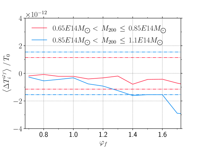
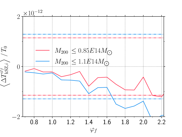
Figure 13: The average AAP filter output from SMICA2018 CMB map at locations of maxBCG clusters below $1.1\times 10^{14}M_{\odot}$, binned in $M_{200}$ (left panel) and cumulative (right panel). The dot-dashed lines represent the typical kSZ signal amplitude of clusters in the $M_{200}$ bin of the same color, assuming a universal $v^{\mathrm{LOS}}=300\,\mathrm{km}\mathrm{s}^{-1}$.

Appendix B The kSZ likelihood: mixture weights, MAP mean and variance of the kSZ signal amplitude

Here, we first derive the individual mixture weight $\lambda_{s}$ for each component of the Gaussian mixture distribution of large-scale bulk-flow amplitude $\alpha_{s}$ in Sec. 3. Let us denote

$$A_{i}=\Delta T_{\mathrm{kSZ},i}/T_{0},$$ (B.1)

and

$$B_{i}^{s}=-\tau_{i}v^{\mathrm{LOS},s}_{L,i}/c.$$ (B.2)

Then, the likelihood on the r.h.s. of Eq. (3.7) can be re-written as

$$\ln\mathcal{P}\left(\{A_{i}\}|\alpha,\,\{B_{i}^{s}\}\right)=-\frac{1}{2}\sum_{i}\left[\frac{A_{i}}{\sigma_{i}}\right]^{2}-\frac{1}{2}\left[\sum_{i}\left(\frac{B_{i}^{s}}{\sigma_{i}}\right)^{2}\right]\,\left[\alpha^{2}-2\alpha\frac{\sum_{i}\frac{A_{i}\,B_{i}^{s}}{\sigma_{i}^{2}}}{\sum_{i}\left(\frac{B_{i}^{s}}{\sigma_{i}}\right)^{2}}\right]-\frac{1}{2}\sum_{i}\ln\left[\sigma_{i}^{2}\right].$$ (B.3)

We further denote

$$\mu_{s}=\frac{\sum_{i}\left[\left(A_{i}\,B_{i}^{s}\right)/\sigma_{i}^{2}\right]}{\sum_{i}\left(B_{i}^{s}/\sigma_{i}\right)^{2}},$$ (B.4)

$$\sigma_{s}^{2}=1/\left[\sum_{i}\left(\frac{B_{i}^{s}}{\sigma_{i}}\right)^{2}\right],$$ (B.5)

$$\gamma=\sum_{i}\left(\frac{A_{i}}{\sigma_{i}}\right)^{2},$$ (B.6)

and

$$\delta=\sum_{i}\ln\left[\sigma_{i}^{2}\right],$$ (B.7)

so that we can shorten Eq. (B.3) to

$$\ln\mathcal{P}=-\frac{1}{2}\gamma+\frac{\mu_{s}^{2}}{2\,\sigma_{s}^{2}}-\frac{1}{2}\delta-\frac{1}{2\,\sigma_{s}^{2}}\,\left(\alpha-\mu_{s}\right)^{2}.$$ (B.8)

The first and third terms on the r.h.s. of Eq. (B.8) neither vary between borg-SDSS3 samples nor depend on $\alpha$, thus they can be dropped from Eq. (B.8), such that

$$\ln\mathcal{P}\propto\frac{1}{2\,\sigma_{s}^{2}}\left[\mu_{s}^{2}-\left(\alpha-\mu_{s}\right)^{2}\right].$$ (B.9)

We can now simply write

$$\mathcal{P}\left(\alpha|\{\Delta T_{\rm kSZ,\it i}/T_{0}\},\{\tau_{i}v^{\rm LOS,\it s}_{L,\it i}/c\}\right)\propto\mathcal{P}(\alpha)\frac{1}{N}\sum_{s}^{N}\mathrm{e}^{\omega_{s}}\,\sqrt{2\pi\,\sigma_{s}^{2}}\frac{\exp\left({-\,\frac{\left(\alpha-\mu_{s}\right)^{2}}{\,2\sigma_{s}^{2}}}\right)}{\sqrt{2\pi\,\sigma_{s}^{2}}}$$ (B.10)

where $\omega_{s}\equiv\frac{\mu^{2}_{s}}{2\sigma^{2}_{s}}$. The normalized version will then be

$$\mathcal{P}\left(\alpha|\{\Delta T_{\rm kSZ,\it i}/T_{0}\},\{\tau_{i}v^{\rm LOS,\it s}_{L,\it i}/c\}\right) =\mathcal{P}(\alpha)\frac{\frac{1}{N}\sum_{s}^{N}\mathrm{e}^{\omega_{s}}\,\sqrt{2\pi\,\left(\sigma_{s}\right)^{2}}\frac{\exp\left(-\frac{\left(\alpha-\mu_{s}\right)^{2}}{\,2\left(\sigma_{s}\right)^{2}}\right)}{\sqrt{2\pi\,\left(\sigma_{s}\right)^{2}}}}{\frac{1}{N}\sum_{s}^{N}\mathrm{e}^{\omega_{s}}\,\sqrt{2\pi\,\left(\sigma_{s}\right)^{2}}}$$ (B.11)

$$=\mathcal{P}(\alpha)\sum_{s}^{N}\lambda_{s}\frac{\exp\left(-\,\frac{\left(\alpha-\mu_{s}\right)^{2}}{\,2\left(\sigma_{s}\right)^{2}}\right)}{\sqrt{2\pi\,\left(\sigma_{s}\right)^{2}}},$$

where

$$\lambda_{s}=\frac{\mathrm{e}^{\omega_{s}\,+\frac{1}{2}\ln\left[2\pi\,\left(\sigma_{s}\right)^{2}\right]}}{\sum_{s}^{N}\mathrm{e}^{\omega_{s}\,+\frac{1}{2}\ln\left[2\pi\,\left(\sigma_{s}\right)^{2}\right]}}.$$ (B.12)

The mean of this distribution can be derived as follows, assuming a uniform prior, i.e. $\mathcal{P}(\alpha)=1$,

$$\langle\alpha\rangle_{s} =\int d\alpha\,\alpha\,\sum_{s}^{N}\lambda_{s}\,\frac{\exp\left(-\,\frac{\left(\alpha-\mu_{s}\right)^{2}}{\,2\left(\sigma_{s}\right)^{2}}\right)}{\sqrt{2\pi\,\left(\sigma_{s}\right)^{2}}}$$ (B.13)

$$=\sum_{s}^{N}\lambda_{s}\,\int d\alpha\,\alpha\,\frac{\exp\left(-\,\frac{\left(\alpha-\mu_{s}\right)^{2}}{\,2\left(\sigma_{s}\right)^{2}}\right)}{\sqrt{2\pi\,\left(\sigma_{s}\right)^{2}}}=\sum_{s}^{N}\lambda_{s}\mu_{s},$$

which is precisely Eq. (3.11).

Similarly, we can explicitly work out the variance of the Gaussian mixture distribution.

$$\sigma^{2}_{\alpha} =\langle\left(\alpha-\langle\alpha\rangle_{s}\right)^{2}\rangle$$ (B.14)

$$=\int d\alpha\,\mathcal{P}\left(\alpha|\{\Delta T_{\mathrm{kSZ},i}/T_{0}\},\{\tau_{i}v^{\mathrm{LOS},s}_{L,i}/c\}\right)\,\left(\alpha-\langle\alpha\rangle_{s}\right)^{2}$$

$$=\sum_{s}^{N}\lambda_{s}\int d\alpha\,\frac{\exp\left(-\,\frac{\left(\alpha-\mu_{s}\right)^{2}}{\,2\left(\sigma_{s}\right)^{2}}\right)}{\sqrt{2\pi\,\left(\sigma_{s}\right)^{2}}}\,\left(\alpha-\langle\alpha\rangle_{s}\right)^{2}$$

$$=\sum_{s}^{N}\lambda_{s}\left(\sigma_{s}\right)^{2}+\sum_{s}^{N}\lambda_{s}\,\left[\left(\mu_{s}-\langle\alpha\rangle_{s}\right)^{2}\right].$$

So the result is the sum of the average noise variances and the variance of the mean estimate (cf. Eq. (3.12)). The second term clearly shows that our uncertainty on $\alpha$ includes also the uncertainty from the velocity reconstruction.

We next compute $\ln\mathcal{P}\left(\{\bm{A_{i}}\}|\alpha,\{\bm{B^{s}_{i}}\}\right)$ for measurements at all $\theta_{f}$ scales in a similar fashion to how we arrived at Eq. (B.11):

$$\ln\mathcal{P}\left(\{\bm{A_{i}}\}|\alpha,\{\bm{B^{s}_{i}}\}\right) =-\frac{1}{2}\sum_{i}\,\left[\bm{A_{i}}-\alpha\bm{B_{i}^{s}}\right]^{\intercal}\,\left(\bm{C}_{i}\right)^{-1}\,\left[\bm{A_{i}}-\alpha\bm{B_{i}^{s}}\right]-\frac{1}{2}\sum_{i}\ln|\bm{C}_{i}|$$ (B.15)

$$\propto-\frac{1}{2}\sum_{i}\left(\bm{B_{i}^{s}}\right)^{\intercal}\,\left(\bm{C_{i}}\right)^{-1}\,\bm{B_{i}^{s}}\left[\alpha^{2}-2\alpha\frac{\sum_{i}\bm{A_{i}}^{\intercal}\,\left(\bm{C_{i}}\right)^{-1}\,\bm{B_{i}^{s}}}{\sum_{i}\left(\bm{B_{i}^{s}}\right)^{\intercal}\,\left(\bm{C_{i}}\right)^{-1}\,\bm{B_{i}^{s}}}\right]$$

where we have omitted terms that do not vary between borg-SDSS3 samples. Eq. (B.15) is similar to Eq. (B.9) with

$$\mu_{s}=\frac{\sum_{i}\bm{A_{i}}^{\intercal}\,\left(\bm{C_{i}}\right)^{-1}\,\bm{B_{i}^{s}}}{\sum_{i}\left(\bm{B_{i}^{s}}\right)^{\intercal}\,\left(\bm{C_{i}}\right)^{-1}\,\bm{B_{i}^{s}}}$$ (B.16)

and

$$\sigma_{s}^{2}=1/\left[\sum_{i}\left(\bm{B_{i}^{s}}\right)^{\intercal}\,\left(\bm{C_{i}}\right)^{-1}\,\bm{B_{i}^{s}}\right].$$ (B.17)

Appendix C CMB contribution to covariance matrix of combined kSZ measurement

We provide here a detailed derivation of the CMB covariance matrix term (cf. Eq. (3.22)) that contributes to the covariance matrix of the combined kSZ measurement described in Sec. 3.2. Let us plug Eq. (3.19) into the first term on the r.h.s. of Eq. (3.18), to obtain

$$\mathbf{C}^{\theta_{f}\theta_{f}^{\prime}}_{\mathrm{CMB},i} =\left(\frac{\pi\theta_{f}\theta^{\prime}_{f}}{T_{0}}\right)^{2}\left\langle\int\frac{d\bm{\ell}}{(2\pi)^{2}}\,\int\frac{d\bm{\ell}^{\prime}}{(2\pi)^{2}}\right.$$ (C.1)

$$\qquad\qquad\qquad\qquad\left.\exp{\left[i\left(\bm{\ell}-\bm{\ell}^{\prime}\right)\cdot\bm{\theta_{i}}\right]}\,\hat{W}\left(\ell\theta_{f}\right)\,\Delta T_{\rm CMB}^{{\mathrm{obs}}}(\bm{\ell})\,\hat{W}\left(\ell^{\prime}\theta^{\prime}_{f}\right)\,\Delta T_{\rm CMB}^{{\mathrm{obs}}}(\bm{\ell}^{\prime})\right\rangle$$

$$=\frac{\pi\theta_{f}^{2}(\theta^{\prime}_{f})^{2}}{2T_{0}^{2}}\,\int_{0}^{\infty}d\ell\,\ell\,\hat{W}\left(\ell\theta_{f}\right)\,\hat{W}\left(\ell\theta_{f}^{\prime}\right)\,C^{\mathrm{CMB}}_{\ell}.$$

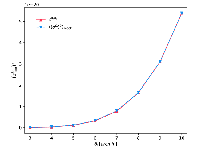
Figure 14: Comparison between analytical (red) and numerical (blue) estimates of CMB contribution to the diagonal of combined kSZ signal covariance matrix.

We further validate the analytical computation of the CMB covariance matrix in Eq. (C.1) by comparing its diagonal elements with the sample variance of $\Delta T_{\mathrm{CMB}}^{\theta_{f}}(\bm{\theta_{i}})/T_{0})$ computed at 1000 random points in each of the 1000 SMICA2018-like CMB mocks in Fig. 14. The analytical calculatrion using the Planck 2018 best-fit $\Lambda$CDM power spectrum is in extremely good agreement with the numerical estimate using SMICA2018-like CMB realizations.

Appendix D GADGET-2 simulation of the borg-SDSS3 volume and mock kSZ signal templates

In order to generate the mock template of kSZ signal within the borg-SDSS3 volume, we use DM particles and halos from a GADGET-2 [51] simulation with DM-only at a very high resolution of $N_{\mathrm{part}}=2048^{3}$. The initial conditions for the simulation is taken from the borg-SDSS3 sample $s=9000$. The halos are identified as main halos by the Rockstar halo finder algorithm [53, 54] with a minimum number of 20 particles per halo. The cosmology and box size of this simulation agree with those of our borg-SDSS3 reconstruction; the initial conditions are specifically taken from sample 9000. The high resolution allows us to achieve a correct halo mass function (HMF) down to $M_{h}=2\times 10^{13}h^{-1}M_{\odot}$ at redshift $z=0.23$, as shown in Fig. 15.

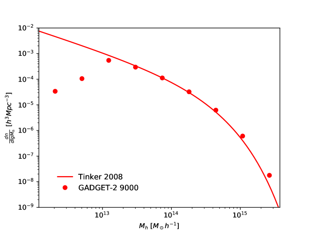
Figure 15: The number density of DM halos identified by Rockstar in our high-resolution GADGET-2 simulation of borg-SDSS3 sample 9000, as compared to the Tinker 2008 halo mass function [63], at redshift $z=0.23$.

For the validity test of our estimator, we model the gas profile of each halo $i$ with a Gaussian profile [see, e.g. 29, 28]:

$$n_{e,i}(\theta)=\frac{N_{e,i}}{\sqrt{2\pi\theta^{2}_{i}}}\exp\left(-\frac{\theta^{2}}{2\theta^{2}_{i}}\right)$$ (D.1)

where $\theta^{2}_{i}=\theta^{2}_{200,i}+\theta^{2}_{\mathrm{beam}}$ and $N_{e,i}=(f_{b}M_{200,i})/(\mu_{e}m_{p})$. For the measurement of the signal profile in Sec. 3.2, we directly generate the kSZ template using all individual DM particles within the same volume analyzed in this work. The LOS velocity of each particle (or halo) is interpolated from the tcola simulation of borg-SDSS3 sample 9000.

References

- [1] R. A. Sunyaev and Y. B. Zeldovich, The Observations of Relic Radiation as a Test of the Nature of X-Ray Radiation from the Clusters of Galaxies, Comments on Astrophysics and Space Physics 4 (1972) 173.
- [2] J. P. Ostriker and E. T. Vishniac, Generation of Microwave Background Fluctuations from Nonlinear Perturbations at the ERA of Galaxy Formation, ApJL 306 (July, 1986) L51.
- [3] P. R. Phillips, Calculation of the Kinetic Sunyaev-Zeldovich Effect from the Boltzmann Equation, ApJ 455 (Dec., 1995) 419.
- [4] M. Birkinshaw, The Sunyaev-Zel’dovich effect, PhR 310 (Mar., 1999) 97–195, [astro-ph/9808050].
- [5] V. Desjacques, D. Jeong and F. Schmidt, Large-scale galaxy bias, PhR 733 (feb, 2018) 1–193, [1611.09787].
- [6] Planck Collaboration, Planck intermediate results - XXXVII. Evidence of unbound gas from the kinetic Sunyaev-Zeldovich effect, A&A 586 (feb, 2016) , [1502.015976].
- [7] M. S. Madhavacheril, N. Battaglia, K. M. Smith and J. L. Sievers, Cosmology with kSZ: breaking the optical depth degeneracy with Fast Radio Bursts, arXiv e-prints (jan, 2019) arXiv:1901.02418, [1901.02418].
- [8] R. Keisler and F. Schmidt, Prospects for measuring the relative velocities of galaxy clusters in photometric surveys using the kinetic Sunyaev-Zel’dovich Effect, ApJL 765 (2013) , [1211.0668].
- [9] Y.-Z. Ma and G.-B. Zhao, Dark energy imprints on the kinematic Sunyaev-Zel’dovich signal, Physics Letters B 735 (jul, 2014) 402–411, [1309.1163].
- [10] E.-M. Mueller, F. de Bernardis, R. Bean and M. D. Niemack, Constraints on gravity and dark energy from the pairwise kinematic Sunyaev-Zeldovich effect, ApJ 808 (jul, 2015) , [1408.6248].
- [11] E.-M. Mueller, F. de Bernardis, R. Bean and M. D. Niemack, Constraints on massive neutrinos from the pairwise kinematic Sunyaev-Zel’dovich effect, PhRvD 92 (sep, 2015) 063501, [1412.0592].
- [12] C. Hernández-Monteagudo, Y.-Z. Ma, F. S. Kitaura, W. Wang, R. Génova-Santos, J. Macías-Pérez et al., Evidence of the Missing Baryons from the Kinematic Sunyaev-Zeldovich Effect in Planck Data, PhRvL 115 (Nov, 2015) 191301, [1504.04011v3].
- [13] S. Lim, H. Mo, H. Wang and X. Yang, The detection of missing baryons in galaxy halos with kinetic Sunyaev-Zel’dovich effect, arXiv e-prints (dec, 2017) arXiv:1712.08619, [1712.08619].
- [14] M. Fukugita, C. J. Hogan and P. J. E. Peebles, The Cosmic Baryon Budget, ApJ 503 (aug, 1998) 518–530, [astro-ph/9712020].
- [15] J. M. Shull, B. D. Smith and C. W. Danforth, The Baryon Census in a Multiphase Intergalactic Medium: 30% of the Baryons May Still be Missing, ApJ 759 (Nov., 2012) 23, [1112.2706].
- [16] F. Nicastro, J. Kaastra, Y. Krongold, S. Borgani, E. Branchini, R. Cen et al., Observations of the missing baryons in the warm-hot intergalactic medium, Nature 558 (June, 2018) 406–409, [1806.08395].
- [17] W. Hu, Reionization Revisited: Secondary Cosmic Microwave Background Anisotropies and Polarization, ApJ 529 (Jan., 2000) 12–25, [astro-ph/9907103].
- [18] C. Dvorkin and K. M. Smith, Reconstructing patchy reionization from the cosmic microwave background, PhRvD 79 (Feb., 2009) 043003, [0812.1566].
- [19] M. A. Alvarez, S. Ferraro, J. C. Hill, R. Hlozek and M. Ikape, Mitigating the optical depth degeneracy using the kinematic Sunyaev-Zel’dovich effect with CMB-S4, arXiv e-prints (June, 2020) arXiv:2006.06594, [2006.06594].
- [20] K. N. Abazajian, P. Adshead, Z. Ahmed, S. W. Allen, D. Alonso, K. S. Arnold et al., CMB-S4 Science Book, First Edition, arXiv e-prints (Oct, 2016) arXiv:1610.02743, [1610.02743].
- [21] M. Levi, C. Bebek, T. Beers, R. Blum, R. Cahn, D. Eisenstein et al., The DESI Experiment, a whitepaper for Snowmass 2013, arXiv e-prints (Aug, 2013) arXiv:1308.0847, [1308.0847].
- [22] Z. Ivezić, S. M. Kahn, J. A. Tyson, B. Abel, E. Acosta, R. Allsman et al., LSST: From Science Drivers to Reference Design and Anticipated Data Products, ApJ 873 (Mar., 2019) 111, [0805.2366].
- [23] M. Münchmeyer, M. S. Madhavacheril, S. Ferraro, M. C. Johnson and K. M. Smith, Constraining local non-Gaussianities with kinetic Sunyaev-Zel’dovich tomography, PhRvD 100 (oct, 2019) 083508, [1810.13424].
- [24] Y.-Z. Ma, Constraining the ionized gas evolution with CMB-spectroscopic survey cross-correlation, Nuclear Physics B 920 (July, 2017) 402–418, [1707.03348].
- [25] N. Hand et al., Evidence of Galaxy Cluster Motions with the Kinematic Sunyaev-Zel’dovich Effect, PhRvL 109 (July, 2012) 041101, [1203.4219].
- [26] B. Soergel et al., Detection of the kinematic Sunyaev-Zel’dovich effect with DES Year 1 and SPT, MNRAS 461 (Sept., 2016) 3172–3193, [1603.03904].
- [27] F. De Bernardis et al., Detection of the pairwise kinematic Sunyaev-Zel’dovich effect with BOSS DR11 and the Atacama Cosmology Telescope, JCAP 2017 (mar, 2017) 008, [1607.02139].
- [28] N. S. Sugiyama, T. Okumura and D. N. Spergel, A direct measure of free electron gas via the kinematic Sunyaev-Zel’dovich effect in Fourier-space analysis, MNRAS (2018) stx3362, [1705.07449].
- [29] E. Schaan et al., Evidence for the kinematic Sunyaev-Zel’dovich effect with the Atacama Cosmology Telescope and velocity reconstruction from the Baryon Oscillation Spectroscopic Survey, PhRvD 93 (Apr., 2016) 082002, [1510.06442].
- [30] H. Tanimura, S. Zaroubi and N. Aghanim, Direct detection of the kinetic Sunyaev-Zel’dovich effect in galaxy clusters, 2007.02952.
- [31] SDSS collaboration, K. N. Abazajian et al., The Seventh Data Release of the Sloan Digital Sky Survey, Astrophys. J. Suppl. 182 (2009) 543–558, [0812.0649].
- [32] BOSS collaboration, L. Anderson et al., The clustering of galaxies in the SDSS-III Baryon Oscillation Spectroscopic Survey: baryon acoustic oscillations in the Data Releases 10 and 11 Galaxy samples, Mon. Not. Roy. Astron. Soc. 441 (2014) 24–62, [1312.4877].
- [33] B. Reid et al., SDSS-III Baryon Oscillation Spectroscopic Survey Data Release 12: galaxy target selection and large scale structure catalogues, Mon. Not. Roy. Astron. Soc. 455 (2016) 1553–1573, [1509.06529].
- [34] J. Jasche and B. D. Wandelt, Bayesian physical reconstruction of initial conditions from large-scale structure surveys, MNRAS 432 (2013) 894–913, [1203.3639].
- [35] J. Jasche and G. Lavaux, Physical Bayesian modelling of the non-linear matter distribution: New insights into the nearby universe, A&A 625 (may, 2019) A64, [1806.11117].
- [36] Planck Collaboration, Planck 2018 results. IV. Diffuse component separation, arXiv e-prints (Jul, 2018) arXiv:1807.06208, [1807.06208].
- [37] B. P. Koester et al., A MaxBCG Catalog of 13,823 Galaxy Clusters from the Sloan Digital Sky Survey, ApJ 660 (May, 2007) 239–255, [astro-ph/0701265].
- [38] G. Lavaux, J. Jasche and F. Leclercq, Systematic-free inference of the cosmic matter density field from SDSS3-BOSS data, arXiv e-prints (sep, 2019) arXiv:1909.06396, [1909.06396].
- [39] J.-F. Cardoso, M. Martin, J. Delabrouille, M. Betoule and G. Patanchon, Component separation with flexible models. Application to the separation of astrophysical emissions, arXiv e-prints (Mar., 2008) arXiv:0803.1814, [0803.1814].
- [40] B. Soergel, A. Saro, T. Giannantonio, G. Efstathiou and K. Dolag, Cosmology with the pairwise kinematic SZ effect: calibration and validation using hydrodynamical simulations, MNRAS 478 (aug, 2018) 5320–5335, [1712.05714].
- [41] M. Li, R. E. Angulo, S. D. M. White and J. Jasche, Matched filter optimization of kSZ measurements with a reconstructed cosmological flow field, MNRAS 443 (2014) 2311–2326, [1404.0007v2].
- [42] E. Rozo et al., Constraining the Scatter in the Mass-richness Relation of maxBCG Clusters with Weak Lensing and X-ray Data, ApJ 699 (jul, 2009) 768–781, [0809.2794].
- [43] D. E. Johnston, E. S. Sheldon, R. H. Wechsler, E. Rozo, B. P. Koester, J. A. Frieman et al., Cross-correlation Weak Lensing of SDSS galaxy Clusters II: Cluster Density Profiles and the Mass–Richness Relation, arXiv e-prints (Sept., 2007) arXiv:0709.1159, [0709.1159].
- [44] K. M. Górski, E. Hivon, A. J. Banday, B. D. Wandelt, F. K. Hansen, M. Reinecke et al., HEALPix: A Framework for High-Resolution Discretization and Fast Analysis of Data Distributed on the Sphere, ApJ 622 (Apr., 2005) 759–771, [arXiv:astro-ph/0409513].
- [45] A. Zonca, L. Singer, D. Lenz, M. Reinecke, C. Rosset, E. Hivon et al., healpy: equal area pixelization and spherical harmonics transforms for data on the sphere in python, Journal of Open Source Software 4 (Mar., 2019) 1298.
- [46] K. S. Dawson et al., The Baryon Oscillation Spectroscopic Survey of SDSS-III, The Astronomical Journal 145 (dec, 2012) 10.
- [47] SDSS-III collaboration, S. Alam et al., The Eleventh and Twelfth Data Releases of the Sloan Digital Sky Survey: Final Data from SDSS-III, Astrophys. J. Suppl. 219 (2015) 12, [1501.00963].
- [48] Y. B. Zel’Dovich, Gravitational instability: an approximate theory for large density perturbations., A&A 500 (Mar., 1970) 13–18.
- [49] T. Buchert, Lagrangian theory of gravitational instability of Friedman-Lemaitre cosmologies and the ’Zel’dovich approximation’, MNRAS 254 (Feb., 1992) 729–737.
- [50] S. Tassev, M. Zaldarriaga and D. J. Eisenstein, Solving large scale structure in ten easy steps with COLA, JCAP 2013 (June, 2013) 036, [1301.0322].
- [51] V. Springel, The cosmological simulation code GADGET-2, MNRAS 364 (Dec., 2005) 1105–1134, [astro-ph/0505010].
- [52] Planck Collaboration, Planck intermediate results. LIII. Detection of velocity dispersion from the kinetic Sunyaev-Zeldovich effect, A&A 617 (Sept., 2018) A48, [1707.00132].
- [53] P. S. Behroozi, R. H. Wechsler and H.-Y. Wu, The ROCKSTAR Phase-space Temporal Halo Finder and the Velocity Offsets of Cluster Cores, ApJ 762 (Jan., 2013) 109, [1110.4372].
- [54] A. Knebe, N. I. Libeskind, F. Pearce, P. Behroozi, J. Casado, K. Dolag et al., Galaxies going MAD: the Galaxy-Finder Comparison Project, MNRAS 428 (Jan., 2013) 2039–2052, [1210.2578].
- [55] Planck Collaboration, Planck 2015 results. VIII. High Frequency Instrument data processing: Calibration and maps, A&A 594 (Sept., 2016) A8, [1502.01587].
- [56] Planck Collaboration, Planck 2018 results. III. High Frequency Instrument data processing and frequency maps, arXiv e-prints (July, 2018) arXiv:1807.06207, [1807.06207].
- [57] Planck Collaboration, Planck 2018 results. VI. Cosmological parameters, arXiv e-prints (July, 2018) arXiv:1807.06209, [1807.06209].
- [58] R. J. Thornton, P. A. R. Ade, S. Aiola, F. E. Angilè, M. Amiri, J. A. Beall et al., The Atacama Cosmology Telescope: The Polarization-sensitive ACTPol Instrument, ApJS 227 (Dec, 2016) 21, [1605.06569].
- [59] J. E. Austermann, K. A. Aird, J. A. Beall, D. Becker, A. Bender, B. A. Benson et al., SPTpol: an instrument for CMB polarization measurements with the South Pole Telescope, vol. 8452 of Society of Photo-Optical Instrumentation Engineers (SPIE) Conference Series, p. 84521E. 2012. 10.1117/12.927286.
- [60] E. Schaan, S. Ferraro, S. Amodeo, N. Battaglia, S. Aiola, J. E. Austermann et al., The Atacama Cosmology Telescope: Combined kinematic and thermal Sunyaev-Zel’dovich measurements from BOSS CMASS and LOWZ halos, arXiv e-prints (Sept., 2020) arXiv:2009.05557, [2009.05557].
- [61] S. Amodeo, N. Battaglia, E. Schaan, S. Ferraro, E. Moser, S. Aiola et al., The Atacama Cosmology Telescope: Modelling the Gas Thermodynamics in BOSS CMASS galaxies from Kinematic and Thermal Sunyaev-Zel’dovich Measurements, arXiv e-prints (Sept., 2020) arXiv:2009.05558, [2009.05558].
- [62] B. A. Benson, P. A. R. Ade, Z. Ahmed, S. W. Allen, K. Arnold, J. E. Austermann et al., SPT-3G: a next-generation cosmic microwave background polarization experiment on the South Pole telescope, in Proc. SPIE, vol. 9153 of Society of Photo-Optical Instrumentation Engineers (SPIE) Conference Series, p. 91531P, July, 2014, 1407.2973, DOI.
- [63] J. Tinker, A. V. Kravtsov, A. Klypin, K. Abazajian, M. Warren, G. Yepes et al., Toward a Halo Mass Function for Precision Cosmology: The Limits of Universality, ApJ 688 (Dec., 2008) 709–728, [0803.2706].