Automated Verification of Reactive and
Concurrent Programs by Calculation

Abstract

Reactive programs combine traditional sequential programming constructs with primitives to allow communication with other concurrent agents. They are ubiquitous in modern applications, ranging from components systems and web services, to cyber-physical systems and autonomous robots. In this paper, we present an algebraic verification strategy for concurrent reactive programs, with a large or infinite state space. We define novel operators to characterise interactions and state updates, and an associated equational theory. With this we can calculate a reactive program’s denotational semantics, and thereby facilitate automated proof. Of note is our reasoning support for iterative programs with reactive invariants, based on Kleene algebra, and for parallel composition. We illustrate our strategy by verifying a reactive buffer. Our laws and strategy are mechanised in Isabelle/UTP, our implementation of Hoare and He’s Unifying Theories of Programming (UTP) framework, to provide soundness guarantees and practical verification support.

1 Introduction

Reactive programming [24, 3] is a paradigm that enables effective description of software systems that exhibit both internal sequential behaviour and event-driven interaction with a concurrent party. Reactive programs are ubiquitous in safety-critical systems, and typically have a very large or infinite state space. Though model checking is an invaluable verification technique, it exhibits inherent limitations with state explosion and infinite-state systems that can be overcome by supplementing it with theorem proving.

Previously [15], we have shown how reactive contracts support an automated verification technique for reactive programs. Reactive contracts follow the design-by-contract paradigm [35], where programs are accompanied by pre- and postconditions. Reactive programs are often non-terminating and so we also capture intermediate behaviours, where the program has not terminated, but is quiescent and offers opportunities to interact. Our contracts are triples, $\left[\,\!P_{1}\!\,\,\scalebox{0.5}[1.0]{$-$}\middle|\,\,\,\!P_{2}\!\,\,\middle|\,\,\!P_{3}\!\,\right]$, where $P_{1}$ is the precondition, $P_{3}$ the postcondition, and $P_{2}$ the pericondition. $P_{2}$ characterises the quiescent observations in terms of the interaction history, and the events enabled at that point. Broadly speaking, our contract theory has its roots in the CSP process algebra [28], and its failures-divergences semantic model [42, 9].

Reactive contracts describe communication and state updates, so $P_{1}$, $P_{2}$, and $P_{3}$ can refer to both a trace history of events and internal program variables. They are, therefore, called “reactive relations”: like relations that model sequential programs, they can refer to variables before ($x$) and later ($x^{\prime}$) in execution, but also the interaction trace (tt), in both intermediate and final observations.

Verification using contracts employs refinement ($\mathrel{\sqsubseteq}$), which allows an implementation to weaken the precondition, and strengthen both the peri- and postcondition when the precondition holds. We employ the “programs-as-predicates” approach [27], where the implementation ($Q$) is itself denoted as a composition of contracts. Thus, a verification problem, $\left[\,\!P_{1}\!\,\,\scalebox{0.5}[1.0]{$-$}\middle|\,\,\,\!P_{2}\!\,\,\middle|\,\,\!P_{3}\!\,\right]\mathrel{\sqsubseteq}Q$, can be solved by calculating a program $\left[\,\!Q_{1}\!\,\,\scalebox{0.5}[1.0]{$-$}\middle|\,\,\,\!Q_{2}\!\,\,\middle|\,\,\!Q_{3}\!\,\right]=Q$, and then discharging three proof obligations: (1) $Q_{1}\mathrel{\sqsubseteq}P_{1}$; (2) $P_{2}\mathrel{\sqsubseteq}(Q_{2}\mathrel{\wedge}P_{1})$; and (3) $P_{3}\mathrel{\sqsubseteq}(Q_{3}\mathrel{\wedge}P_{1})$. These can be further decomposed, using relational calculus, to produce verification conditions. In [15] we employ this strategy in an Isabelle/HOL tactic.

In summary, in our approach verification of reactive programs reduces to reasoning about reactive relations. For programs of a significant size, these relations are complex, and so the resulting proof obligations are difficult to discharge using relational calculus. We need, first, abstract patterns so that the relations can be simplified. This necessitates bespoke constructs that allow us to concisely formulate the three parts of a contract: assumptions, quiescent observations, and terminated observations. Second, we need calculational laws to handle iterative programs, which are only partly handled in our previous work [15].

In this paper we present a novel calculus for description, composition, and simplification of reactive relations in the stateful failures-divergences model [42, 30, 39]. We characterise conditions, external interactions, and state updates. An equational theory allows us to reduce pre-, peri-, and postconditions to compositions of the new constructs using operators of Kleene algebra [32] (KA) and utilise KA proof techniques. Our theory is characterised in the Unifying Theories of Programming [30, 9] (UTP) framework. For that, we identify a class of UTP theories that induce KAs, and utilise it in the derivation of calculational laws for iteration. We use our UTP mechanisation, called Isabelle/UTP [14, 21], to implement an automated verification approach for infinite-state reactive programs with rich data structures based on our calculus.

Our framework can be applied to a wide spectrum of reactive programming languages with trace-based semantics, including real-time and hybrid dynamical systems [26, 54, 46]. A particular focus is languages descended from CSP [28, 42]. In this paper, our approach is applied to the Circus modelling language [52, 39] which combines state modelling using Z [47] and reactive primitives from CSP [28, 42]. An example application is verification of Simulink block diagrams, to which both Circus and hybrid CSP [26] have been successfully applied [8, 55]. More recently, Circus and CSP have been used for verification of a formal state-machine based language for robotic controllers called RoboChart [36, 13].

The paper is structured as follows. §2 outlines preliminary material, including UTP, its mechanisation in Isabelle/UTP, and reactive programs. §3 identifies a class of UTP theories that induce KAs, and applies this class for calculation of iterative contracts. §4 specialises reactive relations with new operators to capture stateful failures-divergences, and derives their equational theory. This allows us to automatically calculate semantics for sequential reactive programs. §5 extends our equational theory with support for calculating external choices, for programs where the environment has control over a decision. We also develop healthiness conditions characterising productivity – a requirement for both algebraic laws of external choice and iteration. §6 extends the strategy with while loops and reactive invariants. §7 encodes parallel composition as a reactive design, and further extends the strategy with calculational laws for concurrent behaviours. With this, we can then calculate semantics for concurrency and communication between reactive processes. §8 demonstrates the resulting proof strategy in a small verification. §9 outlines related work and concludes.

All our theorems, definitions, and proofs have been mechanically verified in Isabelle/UTP, and are documented in a series of technical reports [21, 12, 17, 18]. Additionally, most theorems and definitions in the paper are accompanied by a small Isabelle icon (). In the electronic version, each icon is hyperlinked to the corresponding mechanised artefact in our Isabelle/UTP GitHub repository.

This paper is an extension of [19]. It adds a body of additional theorems in §4 on more specialised healthiness conditions for stateful-failure reactive relations (Theorem 4.3), calculation of iterative reactive relations (Theorem 4.8-(7)), preconditions of reactive contracts (Theorem 4.11), and also extended supporting commentary. Moreover, a substantial new §7 extends the strategy for parallel composition. A number of additional supporting theorems and definitions are also included in the other sections.

2 Preliminaries

This section describes background material relevant for the definition of our new calculus.

2.1 Unifying Theories of Programming

UTP [30, 9] uses the “programs-as-predicates” approach to encode denotational semantics and facilitate reasoning about programs. It uses the alphabetised relational calculus, which combines predicate calculus operators, such as disjunction ($\mathrel{\vee}$), complement ($\neg$), and quantification ($\mathop{\mathstrut{\exists}}\nolimits x\!@P(x)$), with relation algebra [50], to denote programs as binary relations between initial variables ($x$) and their subsequent values ($x^{\prime}$). Here, “alphabetised” means that every such relational predicate is accompanied by a set of declarations of variables to which the predicate can refer. For example, a program fragment, $x:=1\mathrel{\hbox{\rm;}}x:=x+1$, with two distinct variables $x:int$ and $y:bool$, can be modelled by the relational predicate $x^{\prime}=2\mathrel{\wedge}y^{\prime}=y$, with the alphabet $\alpha=\{x:int,x^{\prime}:int,y:bool,y^{\prime}:bool\}$.

In this presentation of the UTP, we first define the set of alphabetised expressions, $[\mathcal{V},\mathcal{S}]\textit{{uexpr}}$, which is parametric over $\mathcal{V}$ and $\mathcal{S}$, types that represent the value type and observation space, respectively. The latter is induced by an alphabet, with a set of typed variable declarations. Expressions are isomorphic to functions $\mathcal{S}\to\mathcal{V}$, which return a value in $\mathcal{V}$ for a given observation space. Alphabetised predicates are represented by Boolean expressions, $[\mathcal{S}]\textit{{upred}}\triangleq[bool,\mathcal{S}]\textit{{uexpr}}$. We denote the set of alphabetised relations by $[\mathcal{S}_{1},\mathcal{S}_{2}]\textit{{urel}}\triangleq[\mathcal{S}_{1}\times\mathcal{S}_{2}]\textit{{upred}}$, a predicate over a product space, where $\mathcal{S}_{1}$ and $\mathcal{S}_{2}$ are the initial and final observation space, and correspond to the sets of undashed and dashed variables, called the input and output alphabets. The set of homogeneous relations $[\mathcal{S}]\textit{{hrel}}\triangleq[\mathcal{S},\mathcal{S}]\textit{{urel}}$ has identical input and output alphabets. We often notationally distinguish predicates over a unitary type and relations over a product type by use of boldface characters; for example, true is a predicate and true is a relation.

For any given $\mathcal{S}_{1}$ and $\mathcal{S}_{2}$, $[\mathcal{S}_{1},\mathcal{S}_{2}]\textit{{urel}}$ is partially ordered by refinement $\mathrel{\sqsubseteq}$ (refined-by), denoting universally closed reverse implication, where false refines every relation. In this context, $S\mathrel{\sqsubseteq}P$ means that $P$ is more deterministic that $S$. For example, we have it that $(x^{\prime}>2)\mathrel{\sqsubseteq}(x:=3)$, since the specification that $x$ should finally have a value greater than $2$ is satisfied by assigning $3$ to $x$.

Every operator of a sequential programming language can be denoted using relations in UTP. Relational composition ($P\mathrel{\hbox{\rm;}}Q$) denotes sequential composition, and has the type $[\mathcal{S}_{1},\mathcal{S}_{2}]\textit{{urel}}\to[\mathcal{S}_{2},\mathcal{S}_{3}]\textit{{urel}}\to[\mathcal{S}_{1},\mathcal{S}_{3}]\textit{{urel}}$, since the output alphabet of the first relation must match the input alphabet of the second. Sequential composition has identity ${\hbox{{I \kern-8.5ptI}}}\triangleq(\hbox{{{s}}}^{\prime}=\hbox{{{s}}})$, of type $[\mathcal{S}]\textit{{hrel}}$, where $\hbox{{{s}}}:\mathcal{S}$ denotes the entire state. We also define the conditional operator $(p\mathop{\hbox{\raisebox{0.0pt}{$\triangleleft$}}}q\mathop{\hbox{\raisebox{0.0pt}{$\triangleright$}}}r)\triangleq((q\mathrel{\wedge}p)\mathrel{\vee}(\neg q\mathrel{\wedge}r))$, with $p,q,r:\textit{{upred}}[\mathcal{S}]$, which selects $p$ or $r$ based on the truth valuation of $q$.

We summarise the algebraic properties of a homogeneous UTP theory of relations in terms of Boolean quantales [37], a useful algebraic structure for characterising homogeneous relations.

Definition 2.1 (Boolean Quantales).

A Boolean quantale [37] is a structure $(S,\leq,0,\cdot,1)$, where $(S,\leq)$ is a complete Boolean lattice with least element $0$; $(S,\cdot,1)$ is a monoid with $0$ as left and right annihilator; and the function $\cdot$ distributes over the lattice join from the left and right.

Theorem 2.2.

For any $\mathcal{S}$, $([\mathcal{S}]\textit{{hrel}},\mathrel{\sqsupseteq},\hbox{{{{false}}}},\mathrel{\hbox{\rm;}},{\hbox{{I \kern-8.5ptI}}})$ is a Boolean quantale [37], so that:

1. $([\mathcal{S}]\textit{{hrel}},\mathrel{\sqsubseteq})$ is a complete lattice, with infimum $\bigvee$, supremum $\bigwedge$, greatest element false, least element true, and weakest (least) fixed-point operator $\mathop{\mathstrut{\mu}}\nolimits F$;

2. $([\mathcal{S}]\textit{{hrel}},\mathrel{\vee},\hbox{{{{false}}}},\mathrel{\wedge},\hbox{{{{true}}}},\neg)$ is a Boolean algebra;

3. $([\mathcal{S}]\textit{{hrel}},\mathrel{\hbox{\rm;}},{\hbox{{I \kern-8.5ptI}}})$ is a monoid with false as left and right annihilator and I I as identity;

4. $\mathrel{\hbox{\rm;}}$ distributes over $\bigvee$ from the left and right.

We emphasise that our complete lattice is inverted compared to several conventions [33, 37], which is normal for UTP [30, 9]. In particular, we often use $\mathop{\mathchoice{\vbox{\hbox{\large$\mathstrut\sqcap$}}}{\vbox{\hbox{\large$\mathstrut\sqcap$}}}{\vbox{\hbox{\small$\mathstrut\sqcap$}}}{\vbox{\hbox{\small$\mathstrut\sqcap$}}}}\nolimits_{i\in I}\,P(i)$ to denote an indexed disjunction over $I$, which intuitively refers to a nondeterministic choice, and likewise $P\mathrel{\sqcap}Q$ to denote $P\mathrel{\vee}Q$. As we have mentioned, refinement reduces nondeterminism, which is illustrated by the following law.

$$\bigsqcap_{i\in I}\,P(i)\,\mathrel{\sqsubseteq}\,\bigsqcap_{j\in J}\,P(j)\textnormal{ when }J\subseteq I$$

In other words, refinement reduces the possible choices that a program is permitted to make. We note that the partial order $\leq$ of the Boolean quantale is $\mathrel{\sqsupseteq}$, and so our lattice operators are inverted: for example, $\bigvee$ is the infimum with respect to $\mathrel{\sqsubseteq}$, and $\mathop{\mathstrut{\mu}}\nolimits F$ is the least fixed-point. More general refinement laws can be found in the work of Back and von Wright [2, Chapter 7].

Relations can be used to denote sequential programming constructs like assignment, and finite and infinite iteration [30, 1]. From these denotations the algebraic laws of programming can be derived [29], along with operational and axiomatic presentations of the semantics [30]. Moreover, relations can be enriched to characterise more advanced computational paradigms — such as object orientation [45], real-time [46], hybrid computation [16], and concurrency [30] — using UTP theories that encode semantic domains.

UTP theories use distinguished observational variables to record observable quantities of the program or operating environment. By their very nature, such variables are not under the control of the programmer, and instead are governed by logical invariants called healthiness conditions. For example, we may introduce variables $time,time^{\prime}:\mathbb{R}_{\geq 0}$ into $\alpha$ to record the time before and after a real-time program fragment executed. We can then define a delay construct, $delay(n)\triangleq time^{\prime}=time+n\mathrel{\wedge}s^{\prime}=s$, where $s$ is shorthand for any variable other than $time$, that advances time whilst leaving all other variables unchanged.

Normally time can only advance, and so a desirable healthiness condition is $time\leq time^{\prime}$, a predicate that any relation modelling a healthy real-time program should respect. The delay construct $delay(n)$ is an example of a healthy relation, and $time=1\mathrel{\wedge}time^{\prime}=0$ is an unhealthy one. We can also prove more general theorems for the other relational operators: for example, if $P$ and $Q$ are both healthy, then also clearly $P\mathrel{\hbox{\rm;}}Q$ is healthy, by transitivity of $\leq$. Similar closure laws can be proved for other operators, which allows us to characterise the signature, or syntax, of our UTP theory: the set of function symbols guaranteed to construct healthy programs when the arguments are healthy.

UTP thus inverts the typical denotational semantic approach of defining an inductive syntax tree, for example using an algebraic datatype, and then giving it a semantics by a recursive function. It has the significant advantages that we can (1) further constrain our semantic domain by adding extra healthiness conditions, in a compositional manner supported by the predicative semantics, and (2) extend the signature with additional syntax when necessary, whilst at the same time retaining all theorems proved with respect to the existing healthiness conditions and operators. Moreover, we avoid the need to perform induction over the syntax tree in our proofs.

A UTP theory can be formally characterised as the set of fixed-points of a function $\hbox{{{{H}}}}:[\mathcal{S}]\textit{{hrel}}\to[\mathcal{S}]\textit{{hrel}}$, that models the healthiness conditions. For example, $\hbox{{{{HT}}}}(P)\triangleq(P\mathrel{\wedge}time\leq time^{\prime})$ is an idempotent healthiness function whose fixed-points are those relations that satisfy $time\leq time^{\prime}$. Any predicate on the observational variables can be encoded as a healthiness function in this way, and therefore we treat the terms healthiness condition and healthiness function as synonyms. If $P$ is a fixed-point of H, it is said to be H-healthy, and the set of healthy relations is $\llbracket\hbox{{{{H}}}}\rrbracket_{\mbox{\tiny{{H}}}}\triangleq\{P|\hbox{{{{H}}}}(P)=P\}$.

In UTP, it is desirable that H is idempotent ($\hbox{{{{H}}}}\!\mathrel{\circ}\!\hbox{{{{H}}}}=\hbox{{{{H}}}}$) and also monotonic ($X\mathrel{\sqsubseteq}Y\mathrel{\Rightarrow}\hbox{{{{H}}}}(X)\mathrel{\sqsubseteq}\hbox{{{{H}}}}(Y)$). Idempotence ensures that, for any $P$, $\hbox{{{{H}}}}(P)$ is indeed H-healthy, and also means that $\llbracket\hbox{{{{H}}}}\rrbracket_{\mbox{\tiny{{H}}}}$ is actually the image of H. Monotonicity additionally ensures, by the Knaster-Tarski theorem, that $\llbracket\hbox{{{{H}}}}\rrbracket_{\mbox{\tiny{{H}}}}$ forms a complete lattice under $\mathrel{\sqsubseteq}$. Consequently, there exist strongest and weakest fixed-points operators, which allow us to reason about both nondeterministic and recursive elements of the UTP theory.

Often, we construct a UTP theory by composition of several healthiness functions, $\hbox{{{{H}}}}_{1}\mathrel{\circ}\hbox{{{{H}}}}_{2}\cdots\mathrel{\circ}\hbox{{{{H}}}}_{n}$. In this case, we can demonstrate idempotence and monotonicity of H using the following important theorem:

Theorem 2.3.

We assume that $\hbox{{{{H}}}}\triangleq\hbox{{{{H}}}}_{1}\mathrel{\circ}\hbox{{{{H}}}}_{2}\cdots\mathrel{\circ}\hbox{{{{H}}}}_{n}$. Then, H is idempotent provided that (1) each $\hbox{{{{H}}}}_{i}$, for $i\in 1..n$ is idempotent, and (2) each pair commutes: for any $i,j\in 1..n$, such that $i\neq j$, $\hbox{{{{H}}}}_{i}\mathrel{\circ}\hbox{{{{H}}}}_{j}=\hbox{{{{H}}}}_{j}\mathrel{\circ}\hbox{{{{H}}}}_{i}$. Moreover, H is monotonic, provided each $\hbox{{{{H}}}}_{i}$ is monotonic.

Consequently, we can reason about a composite healthiness condition in terms of its components. In this paper, we use such a UTP theory to characterise concurrent and reactive programs.

2.2 Isabelle/UTP

Theory engineering and verification using UTP is supported by Isabelle/UTP [14, 21], which provides a shallow embedding of the relational calculus on top of Isabelle/HOL, and various approaches to automated proof. The foundation of Isabelle/UTP is its model of observations, which utilises lenses [11, 14, 21] to model variables as algebraic structures. A lens is a pair of functions $\textit{{get}}:\mathcal{S}\to\mathcal{V}$ and $\textit{{put}}:\mathcal{S}\to\mathcal{V}\to\mathcal{S}$, which are used to query and update a view ($\mathcal{V}$) of a larger observation space ($\mathcal{S}$). We write $X:\mathcal{V}\Longrightarrow\mathcal{S}$ for a lens $X$ viewing $\mathcal{V}$ in the source $\mathcal{S}$, and $\textit{{get}}_{X}$ and $\textit{{put}}_{X}$ for its functions. Typically, $\mathcal{S}$ is characterised by an alphabet of variables ($\alpha$), and consequently we can safely conflate the observation space and alphabet. We characterise the behaviour of each lens using three axioms [11], which link together the functions.

Definition 2.4 (Lens Axioms).

A lens $X:\mathcal{V}\Longrightarrow\mathcal{S}$ satisfies, for any $s:\mathcal{S}$ and $v,v^{\prime}:\mathcal{V}$, the equations

$$\textit{{get}}\,(\textit{{put}}\,s\,v)=v\qquad\textit{{put}}\,(\textit{{put}}\,s\,v^{\prime})\,v=\textit{{put}}\,s\,v\qquad\textit{{put}}\,s\,(\textit{{get}}\,s)=s$$

In this paper, we require that all lenses satisfy these three axioms. We note in passing that these axioms have close analogues in Back and von Wright’s variable calculus [2], which predate lenses by several years. There, get is called val and put is called set, but they are governed by the same axioms. These axioms have several models including record types, total functions, and products [14, 21]. From them, we can characterise the laws of assignment and substitution without dependence on a particular state model. Moreover, we describe semantically when two lenses correspond to different variables, using lens independence [14].

Definition 2.5 (Lens Independence).

We fix $X:\mathcal{V}_{1}\Longrightarrow\mathcal{S}$ and $Y:\mathcal{V}_{2}\Longrightarrow\mathcal{S}$, and then define:

$$X\mathop{\,\bowtie\,}Y\triangleq(\mathop{\mathstrut{\forall}}\nolimits\,s:\mathcal{S},u:\mathcal{V}_{1},v:\mathcal{V}_{2}@\textit{{put}}_{X}(\textit{{put}}_{Y}\,s\,v)\,u\,=\,\textit{{put}}_{Y}(\textit{{put}}_{X}\,s\,u)\,v)$$

$X$ and $Y$ are independent, written $X\mathop{\,\bowtie\,}Y$, provided that their put functions commute, meaning that they do not interfere with one another. Lenses can model, not just individual variables, but also sets thereof. Intuitively, a lens $X:\mathcal{V}\Longrightarrow\mathcal{S}$ abstractly characterises a $\mathcal{V}$-shaped subregion of a $\mathcal{S}$. The lens summation operator [14], $X\oplus Y$, allows us to compose two such independent regions. With it, we can model a set of variables $\{x,y,z\}$ through the summation, $x\oplus y\oplus z$. We also introduce two special lenses [14]:

• $\mathbf{0}:\{\emptyset\}\Longrightarrow\mathcal{S}$, which for any given $\mathcal{S}$, characterises an empty (point) region; and

• $\mathbf{1}:\mathcal{S}\Longrightarrow\mathcal{S}$, which characterises the entirety of $\mathcal{S}$.

We can also use lenses to construct a state by combining the view of one state $s_{2}:\mathcal{S}$ with the complement from another state $s_{1}:\mathcal{S}$. This is useful for merging of parallel threads that act on disjoint parts of the state. We define a novel lens override operator to perform this state merge.

Definition 2.6.

We fix $X:\mathcal{V}\Longrightarrow\mathcal{S}$ and $s_{1},s_{2}:\mathcal{S}$, and define $s_{1}\lhd_{X}s_{2}\triangleq\textit{{put}}_{X}\,s_{1}\,(\textit{{get}}_{X}\,s_{2})$.

Lens override ($s_{1}\lhd_{X}s_{2}$) extracts the region described by $X$ from $s_{2}$ and overwrites the corresponding region in $s_{1}$, leaving the complement unchanged. This operator obeys a number of useful algebraic laws.

Theorem 2.7 (Override Laws).

$$s_{1}\lhd_{\mathbf{0}}s_{2} =s_{1}$$ (1)

$$s_{1}\lhd_{\mathbf{1}}s_{2} =s_{2}$$ (2)

$$s\lhd_{X}s =s$$ (3)

$$(s_{1}\lhd_{X}s_{2})\lhd_{Y}s_{3} =(s_{1}\lhd_{Y}s_{3})\lhd_{X}s_{3} \text{provided }X\mathop{\,\bowtie\,}Y$$ (4)

Law (1) shows that overriding $s_{1}$ with $s_{2}$ using $\mathbf{0}$, the empty lens, effectively means that we use none of $s_{2}$, and (2) is the dual case with the $\mathbf{1}$ lens. Law (3) shows that overriding a source element is idempotent. Law (4) is a kind of commutativity law. In the term $s_{1}\lhd_{X}s_{2}\lhd_{Y}s_{3}$ we are constructing a composite source from the $X$ region of $s_{2}$, the $Y$ region of $s_{3}$, and the remainder from $s_{1}$, with the assumption that $X$ and $Y$ are independent. The law shows that we can, in this case, commute the order in which we apply $s_{2}$ and $s_{3}$.

We can also relate lenses using the sublens preorder [14], $X\preceq Y$, which requires that the view of $X$ is contained within the view of $Y$. For example, $X\preceq X\oplus Y$ – the order is analogous to a subset relation for variable sets: $\{x,y\}\preceq\{x,y,z\}$. Moreover, $\mathbf{0}\preceq X$ and $X\preceq\mathbf{1}$, as these are the smallest and largest lenses.

With lenses, we can also construct substitutions, which are modelled as functions $\sigma:\mathcal{S}\to\mathcal{S}$. They are used in Isabelle/UTP to unify variable substitutions, state updates, assignments, and evaluation contexts, also following the pattern given by Back and von Wright [2]. We can construct substitutions $\llparenthesis x_{1}\mapsto e_{1},x_{2}\mapsto e_{2},\cdots,x_{n}\mapsto e_{n}\rrparenthesis$, which assign an expression $e_{i}:[\mathcal{V}_{i},\mathcal{S}]\textit{{uexpr}}$ to each lens $x_{i}:\mathcal{V}_{i}\Longrightarrow\mathcal{S}$ with a matching view type. Each expression can refer to the previous values of the variables, and variables not mentioned retain their current value. A substitution $\sigma:\mathcal{S}\to\mathcal{S}$ can be applied to an expression $e:[\mathcal{V},\mathcal{S}]\textit{{uexpr}}$ using the operator $\sigma\mathop{\dagger}e\triangleq e\mathrel{\circ}\sigma$, which precomposes the characteristic function of $e$ with the substitution function. We can then define $e[k/x]\triangleq\llparenthesis x\mapsto k\rrparenthesis\mathop{\dagger}e$ to obtain the classical substitution operator. It obeys similar laws to syntactic substitution, though it is a semantic operator [14].

This substitution constructor is syntactic sugar for a more general update operator

$$\sigma(x\mapsto e)\triangleq(\mathop{\mathstrut{\lambda}}\nolimits s@\textit{{put}}_{x}\,(\sigma(s))\,(e(s)))$$

which updates the value of lens $x$ to expression $e$. We can perform several updates using the shorthand

$$\sigma(x_{1}\mapsto e_{1},x_{2}\mapsto e_{2},\cdots,x_{n}\mapsto e_{n})=\sigma(x_{1}\mapsto e_{1})(x_{2}\mapsto e_{2})\cdots(x_{n}\mapsto e_{n})$$

and moreover $\llparenthesis x_{1}\mapsto e_{1},x_{2}\mapsto e_{2},\cdots\rrparenthesis=id(x_{1}\mapsto e_{1})(x_{2}\mapsto e_{2})\cdots$, where $id:\mathcal{S}\to\mathcal{S}$ is the identity substitution. Substitution update obeys several useful laws.

Theorem 2.8 (Substitutions).

We fix $x:\mathcal{V}\Longrightarrow\mathcal{S}$, $y:\mathcal{W}\Longrightarrow\mathcal{S}$, $e:[\mathcal{V},\mathcal{S}]\textit{{uexpr}}$, $f:[\mathcal{W},\mathcal{S}]\textit{{uexpr}}$, $e_{i}:[\mathcal{V}_{i},\mathcal{S}]$ for $1\leq i\leq n$, and $op:[\mathcal{V}_{1},\mathcal{S}]\textit{{uexpr}}\to[\mathcal{V}_{2},\mathcal{S}]\textit{{uexpr}}\cdots\to[\mathcal{V},\mathcal{S}]\textit{{uexpr}}$ and then prove the following laws:

$$\sigma(x\mapsto x) =\sigma$$ (1)

$$\sigma(x\mapsto e,y\mapsto f) =\sigma(y\mapsto f,x\mapsto e) \textnormal{if }x\mathop{\,\bowtie\,}y$$ (2)

$$\sigma(x\mapsto e,y\mapsto f) =\sigma(y\mapsto f) \textnormal{if }x\preceq y$$ (3)

$$\sigma\mathop{\dagger}(op\,e_{1}\cdots e_{n}) =op\,(\sigma\mathop{\dagger}e_{1})\cdots(\sigma\mathop{\dagger}e_{n})$$ (4)

$$\sigma(x\mapsto e)\mathop{\dagger}x =e$$ (5)

An update of a variable to itself has no effect (1). We can commute two updates provided the variables are independent (2). An update to $y$ overrides one to $x$ when $x$ is a narrower lens than $y$, or is equivalent (3). Substitution application distributes through applied operator symbols $op$ (4), and replaces variables with their assigned value (5). These laws provide the foundation for modelling state in a variety of works. In this paper, lenses are valuable in characterising concurrent state updates, as demonstrated in §7.

2.3 Reactive Programs

Whilst sequential programs determine the relationship between an initial and final state, reactive programs also pause during execution to interact with the environment. For example, the CSP [28, 9] and Circus [52, 39] languages can model networks of concurrent processes that communicate using shared channels. Reactive behaviour is described using primitives such as event prefix $a\!\mathrel{\rightarrow}\!P$, which awaits event $a$ and then enables $P$; conditional guard, $b\mathrel{\&}P$, which enables $P$ when $b$ is true; external choice $P\!\mathrel{\Box}\!Q$, where the environment resolves the choice by communicating an initial event of $P$ or $Q$; and iteration $\hbox{{{{while}}}}\,b\,\hbox{{{{do}}}}\,P$. Channels can carry data, and so events can take the form of an input ($c?x$) or output ($c!v$). Circus processes also have local state variables that can be assigned ($x:=e$).

We exemplify the Circus notation with the program for an unbounded buffer.

Example 2.9.

In the $Buffer$ process below, variable $bf:\mathop{\mathrm{seq}}{\mathbb{N}}$ is a finite sequence of natural numbers that records the elements, and channels $inp(n:{\mathbb{N}})$ and $outp(n:{\mathbb{N}})$ represent inputs and outputs.

$$Buffer\,\triangleq\,bf:=\langle\rangle\mathrel{\hbox{\rm;}}\left(\begin{array}[]{l}\hbox{{{{while}}}}\,\,true\,\,\hbox{{{{do}}}}\\ \,\,\begin{array}[]{l}inp?v\mathrel{\rightarrow}bf:=bf\mathbin{\smash{\raise 3.44444pt\hbox{$\smallfrown$}}}\langle v\rangle\\ \mathrel{\Box}(\#bf>0)\mathrel{\&}out!(head(bf))\mathrel{\rightarrow}bf:=tail(bf)\end{array}\end{array}\right)$$

Here, $xs\mathbin{\smash{\raise 3.44444pt\hbox{$\smallfrown$}}}ys$ denotes sequence concatenation [47], and $\langle x,y,z,\cdots\rangle$ denotes an enumerated sequence. Variable $bf$ is set to the empty sequence $\langle\rangle$, and then a non-terminating loop describes the main behaviour. Its body repeatedly allows the environment to either provide a value $v$ over $inp$, followed by which $bf$ is extended, or else, if the buffer is non-empty, receive the value at the head, and then $bf$ is contracted. ∎

Circus has previously been given both a denotational [39] and an operational semantics [53], which are linked in the UTP framework. Here, we build on these previous results and capture the axiomatic semantics for reactive programs using reactive contracts [15]. Reactive contracts can be used both to specify requirements for reactive programs, under certain assumptions, and also to assign denotational semantics to each operator of a reactive programming language. The denotational semantics symbolically encodes the possible transitions a reactive program can exhibit. We can therefore use a theorem prover to reason about a reactive program with a very large or infinite state space. As an example application, we have used them for verifying state-machine diagrams in the RoboChart language [13].

$$\begin{array}[]{rlc|@{\hspace{1ex}}l}\lx@intercol\hfil\textbf{Observational Variable}\hfil\lx@intercol&\hfil\lx@intercol\vrule\hskip 4.30554pt&\lx@intercol\hfil\textbf{Description}\hfil\lx@intercol\\ \hline\cr ok,ok^{\prime}&:\mathbb{B}&\hfil\lx@intercol\vrule\hskip 4.30554pt&\text{Flags whether predecessor or current action has diverged.}\\ wait,wait^{\prime}&:\mathbb{B}&\hfil\lx@intercol\vrule\hskip 4.30554pt&\text{Flags whether predecessor or current action is quiescent.}\\ tr,tr^{\prime},\text{{tt}}&:\mathop{\mathrm{seq}}\textit{Event}&\hfil\lx@intercol\vrule\hskip 4.30554pt&\text{The trace, before, after, and during execution.}\\ \text{{st}},\text{{st}}^{\prime}&:\Sigma&\hfil\lx@intercol\vrule\hskip 4.30554pt&\text{The state, before and after execution.}\\ \text{{ref}}^{\prime}&:\mathop{\mathstrut{\mathbb{P}}}\nolimits(\textit{Event})&\hfil\lx@intercol\vrule\hskip 4.30554pt&\text{The set of events before refused at a quiescent point.}\end{array}$$

Table 1: Overview of Reactive Design Observational Variables

Reactive contracts are built with the following constructor, which is part of our UTP theory’s signature:

$$\left[\,P_{1}(\text{{tt}},\text{{st}},r)\,\,\scalebox{0.5}[1.0]{$-$}\middle|\,\,\,P_{2}(\text{{tt}},\text{{st}},r,r^{\prime})\,\,\middle|\,\,P_{3}(\text{{tt}},\text{{st}},\text{{st}}^{\prime},r,r^{\prime})\,\right]$$

$P_{1}$ is called the precondition, $P_{2}$ is the pericondition, and $P_{3}$ is the postcondition. The notation $P_{i}(x,y,z)$ indicates that relation $P_{i}$ may refer only to $x$, $y$, and $z$ explicitly; any number of variables may be indicated. The variables are modelled as lenses, but for brevity we omit this technicality. Variable tt refers to the trace, which is modelled using a trace algebra [16], and $\text{{st}},\text{{st}}^{\prime}:\Sigma$ to the state, for state space $\Sigma$. Different to the basic relational program model, we follow the pattern of encapsulating all state variables under st to explicitly distinguish them from observational variables [46, 7]. Traces are equipped with operators for the empty trace $\langle\rangle$, concatenation $tt_{1}\mathbin{\smash{\raise 3.44444pt\hbox{$\smallfrown$}}}tt_{2}$, prefix $tt_{1}\leq tt_{2}$, and difference $tt_{1}-tt_{2}$, which removes a prefix $tt_{2}$ from $tt_{1}$. Reactive contracts have an extensible alphabet, and can encode additional semantic data, such as refusals, using extension variables $r,r^{\prime}$, which are placeholders for additional observational variables.

$P_{1-3}$ are reactive relations [15]: a specialised form of homogeneous UTP relation with information about the trace history and state. The different combinations of variables permitted by these relations are constrained using healthiness conditions. These three relations respectively encode, (1) the precondition in terms of the initial state and permissible traces; (2) the pericondition with possible intermediate interactions with respect to an initial state; and (3) the postcondition characterising possible final states should the program terminate. Pericondition $P_{2}$ and postcondition $P_{3}$ are both within the “guarantee” part of the underlying design contract, and so can be strengthened by refinement; see [15] for details. $P_{2}$ does not refer to intermediate state variables since they are concealed when a program is quiescent. We sometimes abbreviate $\left[\,\hbox{{{{true}}}}_{r}\,\,\scalebox{0.5}[1.0]{$-$}\middle|\,\,\,P_{2}\,\,\middle|\,\,P_{3}\,\right]$, a contract with a true precondition, with the notation $\left[\,\!\,\,\scalebox{0.5}[1.0]{$-$}\middle|\,\,\,P_{2}\,\,\middle|\,\,P_{3}\,\right]$. Our precondition corresponds to the “assume” part of a contract. Reactive contracts lie with the greater field of assume-guarantee conditions [4, 5, 44]; a detailed comparison can be found in [15].

In this paper, traces are modelled as finite sequences, $\text{{tt}}:\mathop{\mathrm{seq}}\textit{Event}$, for some set of events given by $Event$, though other models are also admitted [16]. Events can be parametric, written $a.x$, where $a$ is a channel and $x$ is the data. Our theory provides an extensible denotational semantic model for reactive and concurrent languages. To exemplify, we consider the semantics of the skip, event, and assignment actions from Circus, which require that we add variable $\text{{ref}}^{\prime}:\mathop{\mathstrut{\mathbb{P}}}\nolimits(\textit{Event})$ to record refusals, which instantiates the extension variable $r^{\prime}$.

Definition 2.10 (Skip Action, Terminated Event Prefix, and Assignment).

$$\hbox{{{{Skip}}}}\,\,\triangleq\,\,\, \left[\,\hbox{{{{true}}}}_{r}\,\,\scalebox{0.5}[1.0]{$-$}\middle|\,\,\,\hbox{{{{false}}}}\,\,\middle|\,\,\text{{tt}}=\langle\rangle\mathrel{\wedge}\text{{st}}^{\prime}=\text{{st}}\,\right]$$

$$\hbox{{{{Do}}}}(a)\,\,\triangleq\,\,\, \left[\,\hbox{{{{true}}}}_{r}\,\,\scalebox{0.5}[1.0]{$-$}\middle|\,\,\,\text{{tt}}=\langle\rangle\mathrel{\wedge}a\notin\text{{ref}}^{\prime}\,\,\middle|\,\,\text{{tt}}=\langle a\rangle\mathrel{\wedge}\text{{st}}^{\prime}=\text{{st}}\,\right] \text{for }a:[\textit{Event},\Sigma]\textit{{uexpr}}$$

$$x:=e\,\,\triangleq\,\,\, \left[\,\hbox{{{{true}}}}_{r}\,\,\scalebox{0.5}[1.0]{$-$}\middle|\,\,\,\hbox{{{{false}}}}\,\,\middle|\,\,\text{{st}}^{\prime}=\text{{st}}(x\mapsto e)\mathrel{\wedge}\text{{tt}}=\langle\rangle\,\right] \text{for }x:\mathcal{V}\Longrightarrow\Sigma\text{ and }e:[\mathcal{V},\Sigma]\textit{{uexpr}}$$

Each of these contracts specifies the possible behaviours that can be observed in the reactive program. Skip is an action that cannot diverge, and immediately terminates leaving the state unchanged. Its precondition is $\hbox{{{{true}}}}_{r}$, the universal reactive relation (defined below), since it is always satisfied. The pericondition is false because there are no quiescent behaviours. In the postcondition, we define that no events occur ($\text{{tt}}=\langle\rangle$), and the state is left unchanged ($\text{{st}}^{\prime}=\text{{st}}$). The event action ($\hbox{{{{Do}}}}(a)$) also has a true precondition. In the pericondition, we specify that in an intermediate state no events have occurred, but $a$ is not being refused – intuitively this means that the program is waiting to engage in the $a$ event. In the postcondition, we specify that the trace is extended by $a$, since it has now happened, and the state is unchanged. With this we can define the Circus event prefix: $a\mathrel{\rightarrow}P\triangleq\hbox{{{{Do}}}}(a)\mathrel{\hbox{\rm;}}P$. Assignment also has a true precondition, and a false pericondition since it terminates without interaction. The postcondition specifies the updates to the state, and leaves the trace unchanged. This definition of assignment is naturally more expressive than the relational assignment (§2.1) since it also handles observational variables like tt.

As mentioned, reactive contracts can also be used as a specification mechanism. For example, we can define the following contract for deadlock-freedom.

Example 2.11 (Deadlock-freedom Contract).

$\hbox{{{{CDF}}}}\triangleq\textstyle\left[\,\hbox{{{{true}}}}_{r}\,\,\scalebox{0.5}[1.0]{$-$}\middle|\,\,\,\mathop{\mathstrut{\exists}}\nolimits e@e\notin\text{{ref}}^{\prime}\,\,\middle|\,\,\hbox{{{{true}}}}_{r}\,\right]$

CDF requires that every intermediate observation must exhibit at least one enabled event $e$, that is, one event $e$ is not being refused – that is what deadlock-freedom means. The pre- and postcondition do not specify any particular behaviours, since we are only concerned with quiescent observations. Any reactive program that refines CDF must always have an enabled transition. For example, it is the case that $\hbox{{{{CDF}}}}\mathrel{\sqsubseteq}\hbox{{{{Do}}}}(a)$. This can be formally demonstrated using the contract refinement theorem below (Theorem 2.16). First though, we give an overview of the encoding of reactive contracts in UTP.

Following the UTP approach, the constructor $\left[\,P_{1}\,\,\scalebox{0.5}[1.0]{$-$}\middle|\,\,\,P_{2}\,\,\middle|\,\,P_{3}\,\right]$ is really syntactic sugar for a complex relation [15] that is defined using constructs from the UTP theories of reactive processes and designs. Consequently, contracts can be composed using the UTP relational operators. Reactive relations and contracts are characterised by healthiness conditions RR and NSRD, respectively, which we have previously described [15], and reproduce in Table 2. They are all both idempotent and continuous [15]. The observational variables include $ok$ and $wait$, which are used to distinguish normal from divergent behaviour, and quiescent from terminating behaviour, respectively. A summary of all the observational variables is shown in Table 1. A reactive contract is then defined as below.

Definition 2.12.

$\left[\,P_{1}\,\,\scalebox{0.5}[1.0]{$-$}\middle|\,\,\,P_{2}\,\,\middle|\,\,P_{3}\,\right]\triangleq\hbox{{{{R1}}}}\mathrel{\circ}\hbox{{{{R2}}}}\mathrel{\circ}\hbox{{{{R3}}}}_{\!h}(ok\mathrel{\wedge}P_{1}\mathrel{\Rightarrow}ok^{\prime}\mathrel{\wedge}(P_{2}\mathop{\hbox{\raisebox{0.0pt}{$\triangleleft$}}}wait^{\prime}\mathop{\hbox{\raisebox{0.0pt}{$\triangleright$}}}P_{3}))$

This first applies the reactive healthiness conditions, R1, R2, and $\hbox{{{{R3}}}}_{\!h}$ [15]. It then requires that if the predecessor has not diverged ($ok$), and the precondition holds ($P_{1}$), then the contract does not diverge ($ok^{\prime}$). There are then two possibilities: either the contract is quiescent ($wait^{\prime}$), in which case $P_{2}$ holds, otherwise it is terminating ($\neg wait^{\prime}$), in which case $P_{3}$ holds. NSRD specialises the theory of reactive designs [9, 39] to normal stateful reactive designs [15]. This version of reactive designs imposes the requirement that $\text{{st}}^{\prime}$ cannot be referenced in the pericondition, as we assume that quiescent observations do not reveal the state.

Reactive relations characterise the inner elements of a reactive contract, namely the pre-, peri-, and postconditions. Using healthiness conditions called R1 and R2, RR ensures that every observation describes a well-formed trace (tt), and furthermore does not depend on $ok$ or $wait$, as these are only required by the reactive contract infrastructure. Technically, tt is not a relational variable, but a special variable $\text{{tt}}\triangleq tr^{\prime}-tr$ where $tr,tr^{\prime}$, as usual in UTP, encode the trace relationally [30], under the assumption that RR is satisfied. Nevertheless, due to our previous results [21, 16], tt can be treated as a variable, and it is more intuitive to do so. We treat $tr$ and $tr^{\prime}$ as semantic machinery that is concealed in tt, which represents the actual trace.

Preconditions of a reactive contract are elements $\llbracket\hbox{{{{RC}}}}\rrbracket_{\mbox{\tiny{{H}}}}$, which specialises RR by requiring that only the initial state (st) is referenced, and that the trace is prefix closed. The intuition here is that when a trace violates the precondition of a contract, then any extension of this trace must also violate it, similar to how the set of divergences in CSP is extension closed [6]. By duality, if a trace satisfies the precondition, then any prefix of the trace must also satisfy the precondition, and hence the precondition is prefix closed with respect to the trace. The basic reactive relational operators are defined below.

Definition 2.13 (Reactive Relational Operations).

$$\hbox{{{{true}}}}_{r}\triangleq\hbox{{{{R1}}}}(\hbox{{{{true}}}})\qquad(\neg_{r}\,P)\triangleq\hbox{{{{R1}}}}(\neg P)\qquad P\mathop{\mathrel{\Rightarrow}_{\!{r}}}Q\triangleq(\neg_{r}\,P\mathrel{\vee}Q)$$

The theory of reactive relations forms a Boolean algebra, but we have to redefine true, $\neg$, and $\mathrel{\Rightarrow}$ as these are not reactive relations. The relational true is not RR healthy, since it permits any combination of $tr$ and $tr^{\prime}$, and so we define $\hbox{{{{true}}}}_{r}$ to be the least reactive relation. We also need a bespoke complement, $(\neg_{r}\,P)$, because $\llbracket\hbox{{{{RR}}}}\rrbracket_{\mbox{\tiny{{H}}}}$ is similarly not closed under $\neg$. So, after taking the negation, we need to apply R1 to obtain a healthy relation. We also redefine implication for the same reasons ($P\mathop{\mathrel{\Rightarrow}_{\!{r}}}Q$). We do not need to redefine false because, unlike true, it is already RR-healthy, and the same follows for the other logical connectives. We then have proved the following theorem [15].

Theorem 2.14.

$(\llbracket\hbox{{{{RR}}}}\rrbracket_{\mbox{\tiny{{H}}}},\mathrel{\vee},\hbox{{{{false}}}},\mathrel{\wedge},\hbox{{{{true}}}}_{r},\neg_{r}\,)$ forms a Boolean algebra

Both $\llbracket\hbox{{{{RR}}}}\rrbracket_{\mbox{\tiny{{H}}}}$ and $\llbracket\hbox{{{{NSRD}}}}\rrbracket_{\mbox{\tiny{{H}}}}$ are closed under sequential composition, and have units ${\hbox{{I \kern-8.5ptI}}}_{r}$ and ${\hbox{{I \kern-8.5ptI}}}_{\!{\hbox{\tiny\hbox{{{{R}}}}}}}$, respectively, which are defined below

Definition 2.15 (Reactive Relation and Reactive Contract Identities).

$${\hbox{{I \kern-8.5ptI}}}_{r}\triangleq(tr^{\prime}=tr\mathrel{\wedge}\text{{st}}^{\prime}=\text{{st}}\mathrel{\wedge}r^{\prime}=r)\qquad{\hbox{{I \kern-8.5ptI}}}_{\!{\hbox{\tiny\hbox{{{{R}}}}}}}\triangleq((\mathop{\mathstrut{\exists}}\nolimits st@{\hbox{{I \kern-8.5ptI}}})\mathop{\hbox{\raisebox{0.0pt}{$\triangleleft$}}}wait\mathop{\hbox{\raisebox{0.0pt}{$\triangleright$}}}{\hbox{{I \kern-8.5ptI}}})\mathop{\hbox{\raisebox{0.0pt}{$\triangleleft$}}}ok\mathop{\hbox{\raisebox{0.0pt}{$\triangleright$}}}(tr\leq tr^{\prime})$$

${\hbox{{I \kern-8.5ptI}}}_{r}$ is more complex that the basic identity I I. It requires that $tr$, st, and $r$ are unchanged, but leaves the other variables $ok$ and $wait$ unconstrained. We note that ${\hbox{{I \kern-8.5ptI}}}_{\!{\hbox{\tiny\hbox{{{{R}}}}}}}$ and Skip are different operators, as the latter does not restrict ref in the pericondition [15]. Both UTP theories also form complete lattices under $\mathrel{\sqsubseteq}$, with top elements false and $\hbox{{{{Miracle}}}}=\left[\,\!\hbox{{{{true}}}}_{r}\!\,\,\scalebox{0.5}[1.0]{$-$}\middle|\,\,\,\!\hbox{{{{false}}}}\!\,\,\middle|\,\,\!\hbox{{{{false}}}}\!\,\right]$, respectively. Miracle is not a reactive program, but denotes a miraculous or infeasible specification. $\hbox{{{{Chaos}}}}=\left[\,\!\hbox{{{{false}}}}\!\,\,\scalebox{0.5}[1.0]{$-$}\middle|\,\,\,\!\hbox{{{{false}}}}\!\,\,\middle|\,\,\!\hbox{{{{false}}}}\!\,\right]$, the least determinisitic contract, is the bottom of the reactive contract lattice. Any action refines Chaos, and it therefore allows us to denote unspecified or unpredictable behaviour, with the possibility of both termination and non-termination. We define the reactive conditional operator $P\mathop{\hbox{\raisebox{0.0pt}{$\leftslice$}}}b\mathop{\hbox{\raisebox{0.0pt}{$\rightslice$}}}Q$, which specialises the relational conditional operator ($P\mathop{\hbox{\raisebox{0.0pt}{$\triangleleft$}}}b\mathop{\hbox{\raisebox{0.0pt}{$\triangleright$}}}Q$), such that $P$ and $Q$ are reactive relations or contracts, and $b:[\Sigma]\textit{{upred}}$ is a condition on state variables only.

$$\begin{array}[]{rlc|@{\hspace{1ex}}l}\lx@intercol\hfil\textbf{Healthiness Condition}\hfil\lx@intercol&\hfil\lx@intercol\vrule\hskip 4.30554pt&\lx@intercol\hfil\textbf{Description}\hfil\lx@intercol\\ \hline\cr\hbox{{{{R1}}}}(P)&\triangleq P\mathrel{\wedge}tr\leq tr^{\prime}&\hfil\lx@intercol\vrule\hskip 4.30554pt&\text{The trace monotonically increases}\\ \hbox{{{{R2}}}}(P)&\triangleq P[\langle\rangle,tr^{\prime}-tr/tr,tr^{\prime}]\mathop{\hbox{\raisebox{0.0pt}{$\triangleleft$}}}tr\leq tr^{\prime}\mathop{\hbox{\raisebox{0.0pt}{$\triangleright$}}}P&\hfil\lx@intercol\vrule\hskip 4.30554pt&\text{The trace extension is independent of the history}\\ \hbox{{{{R3}}}}_{\!h}(P)&\triangleq{\hbox{{I \kern-8.5ptI}}}_{\!{\hbox{\tiny\hbox{{{{R}}}}}}}\mathop{\hbox{\raisebox{0.0pt}{$\triangleleft$}}}wait\mathop{\hbox{\raisebox{0.0pt}{$\triangleright$}}}P&\hfil\lx@intercol\vrule\hskip 4.30554pt&\text{When a predecessor is quiescent behave as ${\hbox{{I \kern-8.5ptI}}}_{\!{\hbox{\tiny\hbox{{{{R}}}}}}}$}\\ \hbox{{{{RR}}}}(P)&\triangleq(\mathop{\mathstrut{\exists}}\nolimits(ok,ok^{\prime},wait,wait^{\prime})@\hbox{{{{R1}}}}(\hbox{{{{R2}}}}(P)))&\hfil\lx@intercol\vrule\hskip 4.30554pt&\text{Reactive Relations: no references to $ok$ and $wait$}\\ \hbox{{{{RC}}}}(P)&\triangleq\hbox{{{{R1}}}}(\hbox{{{{RR}}}}(P)\mathrel{\hbox{\rm;}}tr^{\prime}\leq tr)&\hfil\lx@intercol\vrule\hskip 4.30554pt&\text{\begin{tabular}[]{l}Reactive Conditions: Reactive Relations where trace\\[-4.30554pt] is prefix closed and there are no references to $\text{{st}}^{\prime}$\end{tabular} }\\ \hbox{{{{SRD1}}}}(P)&\triangleq(ok\mathop{\mathrel{\Rightarrow}_{\!{r}}}P)&\hfil\lx@intercol\vrule\hskip 4.30554pt&\text{Observations are only possible without divergence}\\ \hbox{{{{SRD3}}}}(P)&\triangleq(P\mathrel{\hbox{\rm;}}{\hbox{{I \kern-8.5ptI}}}_{\!{\hbox{\tiny\hbox{{{{R}}}}}}})&\hfil\lx@intercol\vrule\hskip 4.30554pt&\text{Reactive skip is a right unit for $\mathrel{\hbox{\rm;}}$}\\ \hbox{{{{NSRD}}}}&\triangleq\hbox{{{{SRD3}}}}\mathrel{\circ}\hbox{{{{SRD1}}}}\mathrel{\circ}\hbox{{{{R3}}}}_{\!h}\mathrel{\circ}\hbox{{{{R2}}}}\mathrel{\circ}\hbox{{{{R1}}}}&\hfil\lx@intercol\vrule\hskip 4.30554pt&\text{Normal Stateful Reactive Designs}\end{array}$$

Table 2: Overview of Reactive Design Healthiness Conditions

Verification can be facilitated through refinement $\left[\,\!P_{1}\!\,\,\scalebox{0.5}[1.0]{$-$}\middle|\,\,\,\!P_{2}\!\,\,\middle|\,\,\!P_{3}\!\,\right]\mathrel{\sqsubseteq}Q$, where the required property is specified as an explicit contract triple, and the program $Q$ is an NSRD relation. Contract refinement allows the precondition to be weakened, and the peri- and postcondition both to be strengthened [15].

Theorem 2.16 (Reactive Design Refinement).

$\left[\,P_{1}\,\,\scalebox{0.5}[1.0]{$-$}\middle|\,\,\,P_{2}\,\,\middle|\,\,P_{3}\,\right]\mathrel{\sqsubseteq}\left[\,Q_{1}\,\,\scalebox{0.5}[1.0]{$-$}\middle|\,\,\,Q_{2}\,\,\middle|\,\,Q_{3}\,\right]$ if, and only if, $Q_{1}\mathrel{\sqsubseteq}P_{1}$, $P_{2}\mathrel{\sqsubseteq}(Q_{2}\mathrel{\wedge}P_{1})$, and $P_{3}\mathrel{\sqsubseteq}(Q_{3}\mathrel{\wedge}P_{1})$.

Thus, if the contract of the reactive program $Q$ can be calculated to be $\left[\,\!Q_{1}\!\,\,\scalebox{0.5}[1.0]{$-$}\middle|\,\,\,\!Q_{2}\!\,\,\middle|\,\,\!Q_{3}\!\,\right]$, then refinement follows by three proof obligations: (1) $Q_{1}\mathrel{\sqsubseteq}P_{1}$; (2) $P_{2}\mathrel{\sqsubseteq}(Q_{2}\mathrel{\wedge}P_{1})$; and (3) $P_{3}\mathrel{\sqsubseteq}(Q_{3}\mathrel{\wedge}P_{1})$. In words, the precondition may be weakened, and both the peri- and postcondition may be strengthened, assuming the precondition $P_{1}$ holds. As usual, refinement can remove choices, making a contract more deterministic. A consequence is that a non-terminating contract, with postcondition false, can refine a terminating contract. Indeed we have that for any $P$, $P\mathrel{\sqsubseteq}\hbox{{{{Miracle}}}}$. We can avoid refinement by miraculous behaviour by adding feasibility healthiness conditions [30, 9].

In addition to feasibility, refinement does not guarantee to preserve other properties, such as prefix closure of the trace, which is often needed for languages such as CSP [42]. In this case, it is necessary to check these properties of the refined process, or ensure that the process is only constructed of operators that preserve prefix closure, as is the case for CSP. Either way, this check can be conducted separately to the refinement, possibly using a type system, though this is not a concern for this paper.

Contracts can be composed using relational calculus. The following identities [15, 17] show how this entails composition of the underlying pre-, peri-, and postconditions for $\bigsqcap$ and $\mathrel{\hbox{\rm;}}$, and also demonstrate closure of reactive contracts under these operators.

Theorem 2.17 (Reactive Contract Composition).

$$\textstyle\bigsqcap_{i\in I}\,\left[\,\!P_{1}(i)\!\,\,\scalebox{0.5}[1.0]{$-$}\middle|\,\,\,\!P_{2}(i)\!\,\,\middle|\,\,\!P_{3}(i)\!\,\right] =\textstyle\left[\,\bigwedge_{i\in I}P_{1}(i)\,\,\scalebox{0.5}[1.0]{$-$}\middle|\,\,\,\bigvee_{i\in I}P_{2}(i)\,\,\middle|\,\,\bigvee_{i\in I}P_{3}(i)\,\right]$$ (1)

$$\left[\,P_{1}\,\,\scalebox{0.5}[1.0]{$-$}\middle|\,\,\,P_{2}\,\,\middle|\,\,P_{3}\,\right]\mathop{\hbox{\raisebox{0.0pt}{$\leftslice$}}}b\mathop{\hbox{\raisebox{0.0pt}{$\rightslice$}}}\left[\,Q_{1}\,\,\scalebox{0.5}[1.0]{$-$}\middle|\,\,\,Q_{2}\,\,\middle|\,\,Q_{3}\,\right] =\left[\,P_{1}\mathop{\hbox{\raisebox{0.0pt}{$\leftslice$}}}b\mathop{\hbox{\raisebox{0.0pt}{$\rightslice$}}}Q_{1}\,\,\scalebox{0.5}[1.0]{$-$}\middle|\,\,\,P_{2}\mathop{\hbox{\raisebox{0.0pt}{$\leftslice$}}}b\mathop{\hbox{\raisebox{0.0pt}{$\rightslice$}}}Q_{2}\,\,\middle|\,\,P_{3}\mathop{\hbox{\raisebox{0.0pt}{$\leftslice$}}}b\mathop{\hbox{\raisebox{0.0pt}{$\rightslice$}}}Q_{3}\,\right]$$ (2)

$$\left[\,\!P_{1}\!\,\,\scalebox{0.5}[1.0]{$-$}\middle|\,\,\,\!P_{2}\!\,\,\middle|\,\,\!\!P_{3}\!\,\right]\mathrel{\hbox{\rm;}}\left[\,\!Q_{1}\!\,\,\scalebox{0.5}[1.0]{$-$}\middle|\,\,\,\!Q_{2}\!\,\,\middle|\,\,\!\!Q_{3}\!\,\right] =\left[\,\!P_{1}\!\mathrel{\wedge}\!(P_{3}\!\mathop{\,\hbox{{{{wlp}}}}_{r}\,}\!Q_{1})\!\,\,\scalebox{0.5}[1.0]{$-$}\middle|\,\,\,P_{2}\!\mathrel{\vee}\!(P_{3}\!\mathrel{\hbox{\rm;}}\!Q_{2})\!\,\,\middle|\,\,\!P_{3}\!\mathrel{\hbox{\rm;}}\!Q_{3}\,\right]$$ (3)

$$\left[\,\!\,\,\scalebox{0.5}[1.0]{$-$}\middle|\,\,\,P_{2}\,\,\middle|\,\,P_{3}\,\right]\mathrel{\hbox{\rm;}}\left[\,\!\,\,\scalebox{0.5}[1.0]{$-$}\middle|\,\,\,Q_{2}\,\,\middle|\,\,Q_{3}\,\right] =\left[\,\!\,\,\scalebox{0.5}[1.0]{$-$}\middle|\,\,\,P_{2}\!\mathrel{\vee}\!(P_{3}\!\mathrel{\hbox{\rm;}}\!Q_{2})\!\,\,\middle|\,\,\!P_{3}\!\mathrel{\hbox{\rm;}}\!Q_{3}\,\right]$$ (4)

Nondeterministic choice requires all preconditions, and asserts that one of the peri- and postcondition pairs hold. Conditional ($P\mathop{\hbox{\raisebox{0.0pt}{$\leftslice$}}}b\mathop{\hbox{\raisebox{0.0pt}{$\rightslice$}}}Q$) distributes through a reactive contract. For sequential composition, the precondition assumes that $P_{1}$ holds, and that $P_{3}$ does not violate $Q_{1}$. The latter is formulated using a reactive weakest liberal precondition.

Definition 2.18.

$P\mathop{\,\hbox{{{{wlp}}}}_{r}\,}Q\,\triangleq\,\neg_{r}\,(P\mathrel{\hbox{\rm;}}\neg_{r}\,Q)$ where $P\mathop{\,\textit{is}\,}\hbox{{{{RR}}}}$ and $Q\mathop{\,\textit{is}\,}\hbox{{{{RC}}}}$

Intuitively, $P\mathop{\,\hbox{{{{wlp}}}}_{r}\,}Q$ is the weakest reactive condition such that when $P$ terminates, it satisfies $Q$. It obeys standard predicate transformer laws [10, 15] such as:

$$\textstyle(\bigvee_{i\in I}\,P(i))\!\mathop{\,\hbox{{{{wlp}}}}_{r}\,}\!R=\bigwedge_{i\in I}\,(P(i)\!\mathop{\,\hbox{{{{wlp}}}}_{r}\,}\!R)\qquad(P\!\mathrel{\hbox{\rm;}}\!Q)\!\mathop{\,\hbox{{{{wlp}}}}_{r}\,}\!R=P\!\mathop{\,\hbox{{{{wlp}}}}_{r}\,}\!(Q\!\mathop{\,\hbox{{{{wlp}}}}_{r}\,}\!R)\qquad P\mathop{\,\hbox{{{{wlp}}}}_{r}\,}\hbox{{{{true}}}}_{r}=\hbox{{{{true}}}}_{r}$$

In the pericondition of Theorem 2.17-(3), it is specified that an intermediate observation is either of the first contract ($P_{2}$), or else it terminated ($P_{3}$) and then following we have an intermediate observation of the second contract ($Q_{2}$). In the postcondition, the observation specified is for when the contracts have both terminated ($P_{3}\mathrel{\hbox{\rm;}}Q_{3}$). The final law, Theorem 2.17-(4), is a simpler case of the previous law. If both preconditions are true, then since $P_{2}\mathop{\,\hbox{{{{wlp}}}}_{r}\,}\hbox{{{{true}}}}_{r}$ reduces to $\hbox{{{{true}}}}_{r}$, the overall precondition is also $\hbox{{{{true}}}}_{r}$.

With these and related theorems [15], we can calculate contracts of reactive programs. Verification, then, can be performed by proving refinement between two reactive contracts, a strategy we have mechanised in the Isabelle/UTP tactics rdes-refine and rdes-eq [15]. The question remains, though, of how to reason about the underlying compositions of reactive relations for the pre-, peri-, and postconditions. As an example, we consider the action $(a\!\mathrel{\rightarrow}\!\hbox{{{{Skip}}}})\mathrel{\hbox{\rm;}}x\!:=\!v$. To reason about its postcondition, we must simplify $(\text{{tt}}=\langle a\rangle\mathrel{\wedge}\text{{st}}^{\prime}=\text{{st}})\mathrel{\hbox{\rm;}}(\text{{st}}^{\prime}=\text{{st}}(x\mapsto v)\mathrel{\wedge}\text{{tt}}=\langle\rangle)$. To simplify its precondition, we also need to consider reactive weakest preconditions. Without such simplifications, reactive relations can grow very quickly and hamper proof. Of particular importance is the handling of iterative and parallel reactive relations. We address these issues in this paper.

3 Linking UTP and Kleene Algebra

In this section, we characterise properties of a UTP theory sufficient to identify a Kleene Algebra [32], and use this to obtain theorems for iterative contracts. The results in this section apply, not only to stateful-failure reactive designs, but the larger class of reactive designs (NSRD) as well. Consequently, the theorems can be applied in the context of other trace models [16].

Kleene Algebras (KA) characterise sequential and iterative behaviour in nondeterministic programs using a signature $(K,+,0,\cdot,1,{}^{*})$, where $+$ is a choice operator with unit $0$, and $\cdot$ a composition operator, with unit $1$. Kleene closure $P{{}^{*}}$ denotes finite iteration of $P$ using $\cdot$ zero or more times.

We consider the class of weak Kleene algebras [23], which build on weak dioids, as these are the most useful class of Kleene algebra to characterise reactive programs.

Definition 3.1.

A weak dioid is an algebraic structure $(K,+,0,\cdot,1)$ such that $(K,+,0)$ is an idempotent and commutative monoid; $(K,\cdot,1)$ is a monoid; the composition operator $\cdot$ left- and right-distributes over $+$; and $0$ is a left annihilator for $\cdot$.

The $0$ operator represents miraculous behaviour. It is a left annihilator of composition, but not a right annihilator as this often does not hold for programs. $K$ is partially ordered by $x\leq y\triangleq(x+y=y)$, which is defined in terms of $+$, and has least element $0$. A weak KA extends this with the behaviour of the star.

Definition 3.2.

A weak Kleene algebra is a structure $(K\!,+,0,\cdot,1,^{*})$ such that

1. $(K,+,0,\cdot,1)$ is a weak dioid 2. $1+x\cdot x{{}^{*}}\leq x{{}^{*}}$

3. $z+x\cdot y\leq y\mathrel{\Rightarrow}x{{}^{*}}\cdot z\leq y$ 4. $z+y\cdot x\leq y\mathrel{\Rightarrow}z\cdot x{{}^{*}}\leq y$

Various enrichments and specialisations of these axioms exist; for a complete survey see [32]. For our purposes, these axioms alone suffice. From this base, a number of useful identities can be derived:

Theorem 3.3.

$1^{*}=0^{*}=1$  $x{{{}^{*}}{{}^{*}}}=x{{}^{*}}$  $x{{}^{*}}=1+x\cdot x^{*}$  $(x+y){{}^{*}}=(x{{}^{*}}\cdot y{{}^{*}}){{}^{*}}$  $x\cdot x{{}^{*}}=x{{}^{*}}\cdot x$

Kleene Algebra with Tests [33] (KAT) extends the algebra with conditions, and has been successfully applied in program verification [1, 22]. A test is a kind of assumption that entails miraculous behaviour if a condition is violated, and is otherwise ineffectual. The set of tests $T$ are those elements $a,b\in K$ below the identity: $a\leq 1$, over which a Boolean algebra is defined. Tests enjoy a number of additional properties.

Theorem 3.4.

$a\cdot 0=0\quad a\cdot b=b\cdot a\quad a^{*}=1$

UTP relations form a KA $(Rel,\mathrel{\sqcap},\hbox{{{{false}}}},\mathrel{\hbox{\rm;}},{\hbox{{I \kern-8.5ptI}}},^{*})$, where $P^{*}\triangleq(\nu X@{\hbox{{I \kern-8.5ptI}}}\mathrel{\sqcap}P\mathrel{\hbox{\rm;}}X)$. This definition is equivalent to $P^{*}=(\mathop{\mathchoice{\vbox{\hbox{\large$\mathstrut\sqcap$}}}{\vbox{\hbox{\large$\mathstrut\sqcap$}}}{\vbox{\hbox{\small$\mathstrut\sqcap$}}}{\vbox{\hbox{\small$\mathstrut\sqcap$}}}}\nolimits_{i\in{\mathbb{N}}}\,P^{i})$ [20] where $P^{n}$ iterates sequential composition $n$ times. The proof proceeds by application of antisymmetry, the star induction law of Definition 3.2, and the complete lattice theorems.

Typically, UTP theories, like $\llbracket\hbox{{{{NSRD}}}}\rrbracket_{\mbox{\tiny{{H}}}}$, share the operators for choice ($\mathrel{\sqcap}$) and composition ($\mathrel{\hbox{\rm;}}$), only redefining them when absolutely necessary. Formally, given a UTP theory defined by a healthiness condition H, the set of healthy relations $\llbracket\hbox{{{{H}}}}\rrbracket_{\mbox{\tiny{{H}}}}$ is closed under $\mathrel{\sqcap}$ and $\mathrel{\hbox{\rm;}}$. This has the major advantage that a large body of laws is directly applicable from the relational calculus. The ubiquity of $\mathrel{\sqcap}$, in particular, can be characterised through the subset of continuous UTP theories, where H distributes through arbitrary non-empty infima. We formally define this class of healthiness condition below.

Definition 3.5 (Continuous Healthiness Condition).

$$\hbox{{{{H}}}}\left(\mathop{\mathchoice{\vbox{\hbox{\large$\mathstrut\sqcap$}}}{\vbox{\hbox{\large$\mathstrut\sqcap$}}}{\vbox{\hbox{\small$\mathstrut\sqcap$}}}{\vbox{\hbox{\small$\mathstrut\sqcap$}}}}\nolimits_{i\in I}\,P(i)\right)=\mathop{\mathchoice{\vbox{\hbox{\large$\mathstrut\sqcap$}}}{\vbox{\hbox{\large$\mathstrut\sqcap$}}}{\vbox{\hbox{\small$\mathstrut\sqcap$}}}{\vbox{\hbox{\small$\mathstrut\sqcap$}}}}\nolimits_{i\in I}\,\hbox{{{{H}}}}(P(i))\text{ provided }I\neq\emptyset$$

An infinite nondeterministic choice is necessary to support Kleene star iteration. Monotonicity of H follows from continuity, and so such theories induce a complete lattice. Moreover, if H is defined by composition $\hbox{{{{H}}}}_{1}\mathrel{\circ}\hbox{{{{H}}}}_{2}\cdots\mathrel{\circ}\hbox{{{{H}}}}_{n}$, as in Theorem 2.3, then we can show it is continuous by showing each $\hbox{{{{H}}}}_{i}$ is continuous. Continuous UTP theories include designs [30, 23], CSP, and Circus [39]. A consequence of continuity is that the relational weakest fixed-point operator $\mathop{\mathstrut{\mu}}\nolimits X@F(X)$ constructs healthy relations when $F:Rel\to\llbracket\hbox{{{{H}}}}\rrbracket_{\mbox{\tiny{{H}}}}$.

Though these theories share infima and weakest fixed points, they do not, in general, share $\top$ and $\bot$ elements, which is why the infima are non-empty Definition 3.5. Rather, we have a top element $\top\!_{\hbox{\tiny\hbox{{{{H}}}}}}\triangleq\hbox{{{{H}}}}(\hbox{{{{false}}}})$ and a bottom element $\bot\!_{\hbox{\tiny\hbox{{{{H}}}}}}\triangleq\hbox{{{{H}}}}(\hbox{{{{true}}}})$ [15]. The theories also do not share the relational identity I I, but typically define a bespoke identity ${\hbox{{I \kern-8.5ptI}}}_{\hbox{\tiny\hbox{{{{H}}}}}}$, which means that $\llbracket\hbox{{{{H}}}}\rrbracket_{\mbox{\tiny{{H}}}}$ is not closed under the relational Kleene star. However, $\llbracket\hbox{{{{H}}}}\rrbracket_{\mbox{\tiny{{H}}}}$ is closed under Kleene plus, $P^{+}\triangleq P\mathrel{\hbox{\rm;}}P^{*}$, since it is equivalent to $(\mathop{\mathchoice{\vbox{\hbox{\large$\mathstrut\sqcap$}}}{\vbox{\hbox{\large$\mathstrut\sqcap$}}}{\vbox{\hbox{\small$\mathstrut\sqcap$}}}{\vbox{\hbox{\small$\mathstrut\sqcap$}}}}\nolimits_{i\in{\mathbb{N}}}\,P^{i+1})$, which iterates $P$ one or more times. Thus, we can obtain a theory Kleene star with $P\bm{{}^{*}}\triangleq{\hbox{{I \kern-8.5ptI}}}_{\hbox{\tiny\hbox{{{{H}}}}}}\sqcap P^{+}$, under which H is indeed closed. We, therefore, define the following criteria for a UTP theory.

Definition 3.6.

A Kleene UTP theory $(\hbox{{{{H}}}},{\hbox{{I \kern-8.5ptI}}}_{\hbox{\tiny\hbox{{{{H}}}}}})$ satisfies the following conditions: (1) H is idempotent and continuous; (2) H is closed under sequential composition; (3) identity ${\hbox{{I \kern-8.5ptI}}}_{\hbox{\tiny\hbox{{{{H}}}}}}$ is H-healthy; (4) it is a left- and right-unit, ${\hbox{{I \kern-8.5ptI}}}_{\hbox{\tiny\hbox{{{{H}}}}}}\mathrel{\hbox{\rm;}}P=P\mathrel{\hbox{\rm;}}{\hbox{{I \kern-8.5ptI}}}_{\hbox{\tiny\hbox{{{{H}}}}}}=P$, when $P$ is H-healthy; and (5) $\top\!_{\hbox{\tiny\hbox{{{{H}}}}}}\mathrel{\hbox{\rm;}}P=\top\!_{\hbox{\tiny\hbox{{{{H}}}}}}$, when $P$ is H-healthy.

From these properties, we can prove the following theorem.

Theorem 3.7.

If $(\hbox{{{{H}}}},{\hbox{{I \kern-8.5ptI}}}_{\hbox{\tiny\hbox{{{{H}}}}}})$ is a Kleene UTP theory, then $(\llbracket\hbox{{{{H}}}}\rrbracket_{\mbox{\tiny{{H}}}},\mathrel{\sqcap},\top\!_{\hbox{\tiny\hbox{{{{H}}}}}},\mathrel{\hbox{\rm;}},{\hbox{{I \kern-8.5ptI}}}_{\hbox{\tiny\hbox{{{{H}}}}}},\bm{{}^{*}})$ forms a weak Kleene algebra.

Proof.

We prove this in Isabelle/UTP by lifting of laws from the Isabelle/HOL KA hierarchy [1, 22]. For details see [12]. ∎

The identities of Theorem 3.3 hold in a Kleene UTP theory, which allow us to reason about iterative programs. In particular, we can show that $(\llbracket\hbox{{{{NSRD}}}}\rrbracket_{\mbox{\tiny{{H}}}},\mathrel{\sqcap},\hbox{{{{Miracle}}}},\mathrel{\hbox{\rm;}},{\hbox{{I \kern-8.5ptI}}}_{\!{\hbox{\tiny\hbox{{{{R}}}}}}},\bm{{}^{*}})$ and $(\llbracket\hbox{{{{RR}}}}\rrbracket_{\mbox{\tiny{{H}}}},\mathrel{\sqcap},\hbox{{{{false}}}},\mathrel{\hbox{\rm;}},{\hbox{{I \kern-8.5ptI}}}_{r},\bm{{}^{*}})$ both form weak KAs. Moreover, we can now also show how to calculate iterative contracts [17].

Theorem 3.8 (Reactive Contract Iteration).

$$\left[\,P_{1}\,\,\scalebox{0.5}[1.0]{$-$}\middle|\,\,\,P_{2}\,\,\middle|\,\,P_{3}\,\right]\bm{{}^{*}} =\left[\,P_{3}\bm{{}^{*}}\mathop{\,\hbox{{{{wlp}}}}_{r}\,}P_{1}\,\,\scalebox{0.5}[1.0]{$-$}\middle|\,\,\,P_{3}\bm{{}^{*}}\mathrel{\hbox{\rm;}}P_{2}\,\,\middle|\,\,P_{3}\bm{{}^{*}}\,\right]$$

$$\left[\,P_{1}\,\,\scalebox{0.5}[1.0]{$-$}\middle|\,\,\,P_{2}\,\,\middle|\,\,P_{3}\,\right]^{+} =\left[\,P_{3}\bm{{}^{*}}\mathop{\,\hbox{{{{wlp}}}}_{r}\,}P_{1}\,\,\scalebox{0.5}[1.0]{$-$}\middle|\,\,\,P_{3}\bm{{}^{*}}\mathrel{\hbox{\rm;}}P_{2}\,\,\middle|\,\,P_{3}^{+}\,\right]$$

We note that the outer and inner star are different operators. The outer star is formed from the identity ${\hbox{{I \kern-8.5ptI}}}_{\!{\hbox{\tiny\hbox{{{{R}}}}}}}$, and the inner star from ${\hbox{{I \kern-8.5ptI}}}_{r}$. The precondition states that $P_{3}$ must not violate $P_{1}$ after any number of iterations. The pericondition has $P_{3}$ iterated followed by $P_{2}$ holding, since the final observation is intermediate. The postcondition simply iterates $P_{3}$. We also provide a similar law for the Kleene plus operator. It distributes in the same way, except that both the precondition and the pericondition use the star because they must hold before the first iteration; only the postcondition uses the plus.

In this section we have established the basis for calculating and reasoning about iterative reactive contracts. In the next section we specialise our UTP theory to stateful-failure reactive designs, and develop the underlying equational theory. We return to the subject of iteration in Section 6.

4 Reactive Relations of Stateful Failures-Divergences

In this section, we specialise our contract theory to incorporate failure traces, which are used in CSP, Circus, and related languages [54]. We define atomic operators to describe the underlying reactive relations, and the associated equational theory to expand and simplify compositions arising from Theorems 2.17 and 3.8, and thus support automated reasoning. We consider external choice separately (§5).

The failures-divergences model [42] was defined to give a denotational semantics to CSP. It models a process with a pair of sets: $F\subseteq\mathop{\mathstrut{\mathbb{P}}}\nolimits(\mathop{\mathrm{seq}}\,\textit{Event}\,\times\,\mathop{\mathstrut{\mathbb{P}}}\nolimits\,\textit{Event})$ and $D\subseteq\mathop{\mathstrut{\mathbb{P}}}\nolimits(\mathop{\mathrm{seq}}\,\textit{Event})$, which are, respectively, the set of failures and divergences. A failure is a trace of events plus a set of events can be refused at the end of the interaction. A divergence is a trace of events that leads to divergent behaviour, that is, unpredictable behaviour like that of Chaos. A distinguished event $\tick\in Event$ is used as the final element of a trace to indicate that this is a terminating observation. The UTP gives a relational account of the failures-divergences model [30], which was expanded upon by Woodcock and Cavalcanti [9], and by Oliveira [40] to account for state variables in Circus [39]. It is this latter model that we here call the stateful failures-divergences model.

Healthiness condition $\hbox{{{{NCSP}}}}\triangleq\hbox{{{{NSRD}}}}\mathrel{\circ}\hbox{{{{CSP3}}}}\mathrel{\circ}\hbox{{{{CSP4}}}}$ characterises the stateful failures-divergences model [9, 39]. Healthiness conditions CSP3 and CSP4 are defined below.

Definition 4.1 (Stateful-Failure Healthiness Conditions).

$$\hbox{{{{CSP3}}}}(P) \triangleq(\hbox{{{{Skip}}}}\mathrel{\hbox{\rm;}}P) \text{There are no references to $\text{{ref}}$}.$$

$$\hbox{{{{CSP4}}}}(P) \triangleq(P\mathrel{\hbox{\rm;}}\hbox{{{{Skip}}}}) \text{The postcondition may not refer to $\text{{ref}}^{\prime}$}.$$

CSP3 and CSP4 ensure the refusal sets are well-formed [9, 30]: $\text{{ref}}^{\prime}$ can be mentioned only in the pericondition, since refusals are only observed in quiescent observations. NCSP, like NSRD, is continuous and has Skip as a left and right unit. Thus, it fulfils the criteria of a Kleene UTP theory (Definition 3.7), and consequently $(\llbracket\hbox{{{{NCSP}}}}\rrbracket_{\mbox{\tiny{{H}}}},\mathrel{\sqcap},\hbox{{{{Miracle}}}},\mathrel{\hbox{\rm;}},\hbox{{{{Skip}}}},\bm{{}^{*}})$ forms a Kleene algebra. Every NCSP-healthy relation corresponds to a reactive contract with the following specialised form [18].

$$\left[\,P_{1}(\text{{tt}},\text{{st}})\,\,\scalebox{0.5}[1.0]{$-$}\middle|\,\,\,P_{2}(\text{{tt}},\text{{st}},\text{{ref}}^{\prime})\,\,\middle|\,\,P_{3}(\text{{tt}},\text{{st}},\text{{st}}^{\prime})\,\right]$$

The underlying reactive relations capture a portion of the stateful failures-divergences. $P_{1}$ is the precondition, which captures the initial states and traces that do not induce divergence. It corresponds to the the complement of $D$, the set of divergences [42, 9]. $P_{2}$ is the pericondition, which captures the stateful failures of a program: the set of events that may be refused ($\text{{ref}}^{\prime}$) having performed trace tt, starting in state st. It corresponds to the the failure traces in $F$ that are not terminating. $P_{3}$ captures the terminated behaviours, where a final state is observed but no refusals. It, of course, corresponds to the traces in $F$ that have as the final element. We now characterise these reactive relations using healthiness conditions.

Definition 4.2.

Stateful-failure Reactive Relations, Finalisers, and Conditions are characterised as fixed-points of the healthiness conditions CRR, CRF, and CRC defined below.

$$\hbox{{{{CRR}}}}(P)\triangleq\mathop{\mathstrut{\exists}}\nolimits\text{{ref}}@\hbox{{{{RR}}}}(P)\qquad\hbox{{{{CRF}}}}(P)\triangleq\mathop{\mathstrut{\exists}}\nolimits(\text{{ref}},\text{{ref}}^{\prime})@\hbox{{{{RR}}}}(P)\qquad\hbox{{{{CRC}}}}(P)\triangleq\mathop{\mathstrut{\exists}}\nolimits\text{{ref}}@\hbox{{{{RC}}}}(P)$$

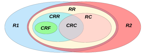
Figure 1: Reactive Relational Healthiness Conditions Venn diagram

These are straightforward extensions of the healthiness conditions for reactive relations (RR) and conditions (RC) that we previously defined [15] and are presented in Table 2. In addition to requiring that the relations describe a well-formed trace, CRR, CRF, and CRC require that there is no reference to ref, because there is never a dependence on the refusal set of a predecessor. Reactive finalisers (CRF) additionally forbid reference to $\text{{ref}}^{\prime}$: they are used to characterise postconditions in a stateful-failure reactive contracts. Every CRF-healthy relation is also CRR-healthy; further containments are shown in Figure 1. We can formally characterise NCSP contracts with the following theorem.

Theorem 4.3.

$\left[\,P_{1}\,\,\scalebox{0.5}[1.0]{$-$}\middle|\,\,\,P_{2}\,\,\middle|\,\,P_{3}\,\right]$ is NCSP-healthy if the following conditions are satisfied:

1. $P_{1}$ is CRC-healthy;

2. $P_{2}$ is CRR-healthy;

3. $P_{2}$ does not refer to $\text{{st}}^{\prime}$; and

4. $P_{3}$ is CRF-healthy.

Due to the restrictions on ref, ${\hbox{{I \kern-8.5ptI}}}_{r}$ is not CRR-healthy, and so we define the identity relation below.

Definition 4.4.

${\hbox{{I \kern-8.5ptI}}}_{\mbox{\tiny{c}}}\triangleq(\text{{st}}^{\prime}=\text{{st}}\mathrel{\wedge}tr^{\prime}=tr)$

This identity specifies only that the trace and state remain unchanged, whilst ref is unspecified. This is different to ${\hbox{{I \kern-8.5ptI}}}_{r}$ which has $\text{{ref}}^{\prime}=\text{{ref}}$ because $r$ is specialised to ref (see Definition 2.15). Consequently, ${\hbox{{I \kern-8.5ptI}}}_{\mbox{\tiny{c}}}$ is indeed CRF-healthy. ${\hbox{{I \kern-8.5ptI}}}_{\mbox{\tiny{c}}}$ is a left unit for CRR, CRF, and CRC-healthy relations, but it is a right unit only for CRF. This is because in $P\mathrel{\hbox{\rm;}}{\hbox{{I \kern-8.5ptI}}}_{\mbox{\tiny{c}}}$, if $P$ refers to $\text{{ref}}^{\prime}$ then this information is lost, whilst CRF relations do not refer to $\text{{ref}}^{\prime}$. We can construct a Kleene algebra for CRF-healthy relations.

Theorem 4.5.

$(\llbracket\hbox{{{{CRF}}}}\rrbracket_{\mbox{\tiny{{H}}}},\mathrel{\sqcap},\hbox{{{{false}}}},\mathrel{\hbox{\rm;}},{\hbox{{I \kern-8.5ptI}}}_{\mbox{\tiny{c}}},\bm{{}^{*}})$ forms a weak Kleene algebra.

Using the Kleene star operators for NCSP and CRF, we can also revalidate Theorem 3.8 in this context. This is necessary because the star in Theorem 3.8 is defined in terms of ${\hbox{{I \kern-8.5ptI}}}_{r}$ and not ${\hbox{{I \kern-8.5ptI}}}_{\mbox{\tiny{c}}}$. Nevertheless the two star operators are strongly related, and so we need only to slightly adapt the proof.

Having defined our theories of stateful-failure reactive relations, we now proceed to define operators for constructing pre-, peri-, and postconditions. These operators allow us to describe a distinct pattern for the form of reactive programs. We describe this pattern using the following constructs.

Definition 4.6 (Reactive Relational Operators).

$$\begin{array}[]{lrcl}\text{Assumption:}&\mathcal{I}\!\left[s(\text{{st}}),t(\text{{st}})\right]&\triangleq&\hbox{{{{CRC}}}}(s(\text{{st}})\mathop{\mathrel{\Rightarrow}_{\!{r}}}\neg_{r}\,(t(\text{{st}})\leq\text{{tt}}))\\[0.86108pt] \text{Quiescence:}&\mathcal{E}\!\left[s(\text{{st}}),t(\text{{st}}),E(\text{{st}})\right]&\triangleq&\hbox{{{{CRR}}}}(s(\text{{st}})\mathrel{\wedge}\text{{tt}}=t(\text{{st}})\mathrel{\wedge}(\mathop{\mathstrut{\forall}}\nolimits e\!\in\!E(\text{{st}})@e\notin\text{{ref}}^{\prime}))\\[0.86108pt] \text{Finalisation:}&\Phi\!\left[s(\text{{st}}),\sigma,t(\text{{st}})\right]&\triangleq&\hbox{{{{CRR}}}}(s(\text{{st}})\mathrel{\wedge}\text{{st}}^{\prime}=\sigma(\text{{st}})\mathrel{\wedge}\text{{tt}}=t(\text{{st}}))\end{array}$$

We utilise expressions $s$, $t$, and $E$ that refer only to the variables indicated. Namely, $s\!:\!\mathbb{B}$ is a condition on st, $t\!:\!\mathop{\mathrm{seq}}\textit{Event}$ is a trace expression that describes an event sequence in terms of st, and $E:\mathop{\mathstrut{\mathbb{P}}}\nolimits\textit{Event}$ describes a set of events. The use of trace expressions allows us to handle symbolic traces that contain free state variables, and characterise a potentially infinite number of traces with a finite presentation. With this, we can calculate semantics for reactive programs with an infinite number of states.

$\mathcal{I}\!\left[s(\text{{st}}),t(\text{{st}})\right]$ is a CRC-healthy reactive condition that is used to specify assumptions on the state and trace in preconditions. It states that, if the state initially satisfies condition $s$, then $t$ is not a prefix of the overall trace. For example, the assumption $\mathcal{I}\!\left[x>2,\langle a,b\rangle\right]$ means that if the state variable $x$ is initially greater than 2, then we disallow the trace $\langle a,b\rangle$, and any extension thereof. The intuition here is that $t$ is a trace that introduces divergence, and so any extension of $t$ violates the precondition. Put another way, any trace that is a either strict prefix or orthogonal to $t$ satisfies the precondition when $s$ holds. Effectively, $t$ sets a strict upper bound on the traces permitted by the precondition.

$\mathcal{E}\!\left[s(\text{{st}}),t(\text{{st}}),E(\text{{st}})\right]$ is used in periconditions to specify quiescent observations, and corresponds to a set of symbolic failure traces. It specifies that the state variables initially satisfy $s$, the interaction described by $t$ has occurred, and finally we reach a quiescent phase where none of the events in $E$ are being refused. It has the form of an acceptance trace [42], as this provides a more comprehensible presentation, but the semantics is encoded as a collection of failure traces. Specifically, $(\mathop{\mathstrut{\forall}}\nolimits e\!\in\!E(\text{{st}})@e\notin\text{{ref}}^{\prime})$ defines all possible refusals that satisfy symbolic acceptance set $E$. We sometimes write $\mathcal{E}\!\left[t(\text{{st}}),E(\text{{st}})\right]$ when $s$ is true.

$\Phi\!\left[s(\text{{st}}),\sigma,t(\text{{st}})\right]$ is used in postconditions to specify final terminated observations. It specifies that the initial state satisfies $s$, the state update $\sigma$ is applied to update st, and the symbolic interaction $t$ has occurred. Since $\Phi\!\left[s,\sigma,t\right]$ does not refer to $\text{{ref}}^{\prime}$, it is CRF-healthy. We sometimes write $\Phi\!\left[\sigma,t(\text{{st}})\right]$ in the case that $s$ is true. Moreover, we also introduce the abbreviation $[s]_{c}\triangleq\Phi\!\left[s,id,\langle\rangle\right]$ that denotes a reactive relational test (or assumption) on the state of the property $s$.

These operators are all deterministic, in the sense that they describe a single interaction and state-update history. There is no need for explicit nondeterminism here, as this is achieved using $\bigvee$. These operators allow us to concisely specify the basic operators of our theory as given below.

Definition 4.7 (Basic Reactive Operators).

$$\langle\sigma\rangle_{\hbox{\tiny\hbox{{{{C}}}}}}\,\triangleq\, \left[\,\hbox{{{{true}}}}_{r}\,\,\scalebox{0.5}[1.0]{$-$}\middle|\,\,\,\hbox{{{{false}}}}\,\,\middle|\,\,\Phi\!\left[\textit{{true}},\sigma,\langle\rangle\right]\,\right]$$ (1)

$$\hbox{{{{Skip}}}}\,=\, \langle id\rangle_{\hbox{\tiny\hbox{{{{C}}}}}}$$ (2)

$$\hbox{{{{Do}}}}(a)\,=\, \left[\,\hbox{{{{true}}}}_{r}\,\,\scalebox{0.5}[1.0]{$-$}\middle|\,\,\,\mathcal{E}\!\left[\textit{{true}},\langle\rangle,\{a\}\right]\,\,\middle|\,\,\Phi\!\left[\textit{{true}},id,\langle a\rangle\right]\,\right]$$ (3)

$$\hbox{{{{Stop}}}}\,\triangleq\, \left[\,\hbox{{{{true}}}}_{r}\,\,\scalebox{0.5}[1.0]{$-$}\middle|\,\,\,\mathcal{E}\!\left[\textit{{true}},\langle\rangle,\emptyset\right]\,\,\middle|\,\,\hbox{{{{false}}}}\,\right]$$ (4)

The definitions of Skip and $\hbox{{{{Do}}}}(a)$ are expressed as theorems that we have proved using Definition 2.10. However, for the remainder of this paper we treat these identities as definitions. Generalised assignment $\langle\sigma\rangle_{\hbox{\tiny\hbox{{{{C}}}}}}$ is again inspired by [2]. It has a $\hbox{{{{true}}}}_{r}$ precondition and a false pericondition: it has no intermediate observations. The postcondition states that for any initial state (true), the state is updated using $\sigma$, and no events are produced ($\langle\rangle$). A singleton assignment $x:=v$ can be expressed using $\langle x\mapsto v\rangle_{\hbox{\tiny\hbox{{{{C}}}}}}$. We can use it to show that $\hbox{{{{Skip}}}}=\langle id\rangle_{\hbox{\tiny\hbox{{{{C}}}}}}$, where $id:\Sigma\to\Sigma$ is the identity function that leaves all variables unchanged.

$\hbox{{{{Do}}}}(a)$ encodes an event action. Its pericondition states that no event has occurred, and $a$ is accepted. Its postcondition extends the trace by $a$, leaving the state unchanged. We can denote Circus event prefix $a\mathrel{\rightarrow}P$ as $\hbox{{{{Do}}}}(a)\mathrel{\hbox{\rm;}}P$. Finally, Stop represents a deadlock: its pericondition states the trace is unchanged and no events are being accepted. The postcondition is false as there is no way to terminate. A Circus guard $g\mathrel{\&}P$ can be denoted as $(P\mathop{\hbox{\raisebox{0.0pt}{$\leftslice$}}}g\mathop{\hbox{\raisebox{0.0pt}{$\rightslice$}}}\hbox{{{{Stop}}}})$, which behaves as $P$ when $g$ is true, and otherwise deadlocks.

To calculate contractual semantics, we need laws to reduce pre-, peri-, and postconditions. These need to cater for compositions of quiescent and final observations using operators like internal choice ($\bigsqcap$), sequential composition ($\mathrel{\hbox{\rm;}}$), and external choice ($\mathop{\mathchoice{\vbox{\hbox{\large$\mathstrut\Box$}}}{\vbox{\hbox{\large$\mathstrut\Box$}}}{\vbox{\hbox{\small$\mathstrut\Box$}}}{\vbox{\hbox{\small$\mathstrut\Box$}}}}\nolimits$, see §5). So, we prove [18] the following laws for $\mathcal{E}$ and $\Phi$.

Theorem 4.8 (Reactive Relational Compositions).

$$\Phi\!\left[\textit{{true}},id,\langle\rangle\right] ={\hbox{{I \kern-8.5ptI}}}_{\mbox{\tiny{c}}}$$ (1)

$$\Phi\!\left[s_{1},\sigma_{1},t_{1}\right]\mathrel{\hbox{\rm;}}\Phi\!\left[s_{2},\sigma_{2},t_{2}\right] =\Phi\!\left[s_{1}\mathrel{\wedge}\sigma_{1}\mathop{\dagger}s_{2},\sigma_{2}\mathrel{\circ}\sigma_{1},t_{1}\mathbin{\smash{\raise 3.44444pt\hbox{$\smallfrown$}}}\sigma_{1}\mathop{\dagger}t_{2}\right]$$ (2)

$$\Phi\!\left[s_{1},\sigma_{1},t_{1}\right]\mathrel{\hbox{\rm;}}\mathcal{E}\!\left[s_{2},t_{2},E\right] =\mathcal{E}\!\left[s_{1}\mathrel{\wedge}\sigma_{1}\mathop{\dagger}s_{2},t_{1}\mathbin{\smash{\raise 3.44444pt\hbox{$\smallfrown$}}}\sigma_{1}\mathop{\dagger}t_{2},\sigma_{1}\mathop{\dagger}E\right]$$ (3)

$$\Phi\!\left[s_{1},\sigma_{1},t_{1}\right]\mathop{\hbox{\raisebox{0.0pt}{$\leftslice$}}}c\mathop{\hbox{\raisebox{0.0pt}{$\rightslice$}}}\Phi\!\left[s_{2},\sigma_{2},t_{2}\right] =\Phi\!\left[s_{1}\mathop{\hbox{\raisebox{0.0pt}{$\leftslice$}}}c\mathop{\hbox{\raisebox{0.0pt}{$\rightslice$}}}s_{2},\sigma_{1}\mathop{\hbox{\raisebox{0.0pt}{$\leftslice$}}}c\mathop{\hbox{\raisebox{0.0pt}{$\rightslice$}}}\sigma_{2},t_{1}\mathop{\hbox{\raisebox{0.0pt}{$\leftslice$}}}c\mathop{\hbox{\raisebox{0.0pt}{$\rightslice$}}}t_{2}\right]$$ (4)

$$\mathcal{E}\!\left[s_{1},t_{1},E_{1}\right]\mathop{\hbox{\raisebox{0.0pt}{$\leftslice$}}}c\mathop{\hbox{\raisebox{0.0pt}{$\rightslice$}}}\mathcal{E}\!\left[s_{2},t_{2},E_{2}\right] =\mathcal{E}\!\left[s_{1}\mathop{\hbox{\raisebox{0.0pt}{$\leftslice$}}}c\mathop{\hbox{\raisebox{0.0pt}{$\rightslice$}}}s_{2},t_{1}\mathop{\hbox{\raisebox{0.0pt}{$\leftslice$}}}c\mathop{\hbox{\raisebox{0.0pt}{$\rightslice$}}}t_{2},E_{1}\mathop{\hbox{\raisebox{0.0pt}{$\leftslice$}}}c\mathop{\hbox{\raisebox{0.0pt}{$\rightslice$}}}E_{2}\right]$$ (5)

$$\left(\bigwedge_{i\in I}\,\mathcal{E}\!\left[s(i),t,E(i)\right]\right) =\mathcal{E}\!\left[\bigwedge_{i\in I}\,s(i),t,\bigcup_{i\in I}\,E(i)\right]$$ (6)

$$\left(\bigvee_{i\in I}\,\mathcal{E}\!\left[s(i),t,E(i)\right]\right) =\mathcal{E}\!\left[\bigvee_{i\in I}\,s(i),t,\bigcap_{i\in I}\,E(i)\right]$$ (7)

$$\Phi\!\left[s,\sigma,t\right]^{{}^{*}} =\bigsqcap_{n\in{\mathbb{N}}}\,\Phi\!\left[\bigwedge_{i\leq n}(\sigma^{i}\mathop{\dagger}s),\sigma^{n},\prod_{j<n}\,(\sigma^{j}\mathop{\dagger}t)\right]$$ (8)

Law (1) gives the meaning of $\Phi$ with a trivial precondition, state update, and empty trace: it is simply the reactive identity. Law (2) states that the composition of two terminated observations results in the conjunction of the state conditions, composition of the state updates, and concatenation of the traces. It is necessary to apply the initial state update $\sigma_{1}$ as a substitution to both the second state condition ($s_{2}$) and the trace expression ($t_{2}$). Law (3) is similar, but accounts for the enabled events rather than state updates. Laws (2) and (3) are required because of Theorem 2.17-(3), which sequentially composes a pericondition with a postcondition, and a postcondition with a postcondition.

Laws (4) and (5) show how conditional distributes through the operators. Law (6) shows that a conjunction of intermediate observations with a common trace corresponds to the conjunction of the state conditions, and the union of the enabled events. It is needed for external choice, which conjoins the periconditions (see §5). Law (7) shows the dual case of (6): when taking a choice of periconditions, we have the disjunction of all the state conditions, and intersection of all enabled events.

Finally, (8) gives the meaning of an iterated final observation. The nondeterministic choice over $n\in{\mathbb{N}}$ denotes the number of iterations. Inside, the $\Phi$ operator distributes iteration though the condition, state updates, and trace. Here, $f^{n}$ is iterated function composition ($f\mathrel{\circ}f\mathrel{\circ}f\cdots$), and $\prod$ is iterated concatenation:

$$\prod_{i<n}\,xs(i)\triangleq xs(0)\mathbin{\smash{\raise 3.44444pt\hbox{$\smallfrown$}}}xs(1)\mathbin{\smash{\raise 3.44444pt\hbox{$\smallfrown$}}}\cdots\mathbin{\smash{\raise 3.44444pt\hbox{$\smallfrown$}}}xs(n-1)$$

The condition of an iterated final observation requires that $s$ holds whenever $\sigma$ is applied as a substitution $i$ times, where $i\leq n$. The state update applies $\sigma$ a total of $n$ times in sequence. The trace expression concatenates $t$ a total of $n$ times, and each instance has the state update applied $j<n$ times.

We can now use these laws, along with Theorem 2.17, to calculate the semantics of processes, and to prove equality and refinement conjectures, as we illustrate below.

Example 4.9.

We show that $(x\!:=\!1\mathrel{\hbox{\rm;}}\hbox{{{{Do}}}}(a.x)\mathrel{\hbox{\rm;}}x:=x+2)\,=\,(\hbox{{{{Do}}}}(a.1)\mathrel{\hbox{\rm;}}x\!:=\!3)$. By applying Definition 4.7 and Theorems 2.17-(3), 4.8, 4.11, both sides reduce to $\,\left[\,\!\,\,\scalebox{0.5}[1.0]{$-$}\middle|\,\,\,\mathcal{E}\!\left[true,\langle\rangle,\{a.1\}\right]\,\,\middle|\,\,\Phi\!\left[true,\{x\mapsto 3\},\langle a.1\rangle\right]\,\right]$, which has a single quiescent state, waiting for event $a.1$, and a single final state, where $a.1$ has occurred and state variable $x$ has been updated to $3$. We calculate the left-hand side below.

$$(x\!:=\!1\mathrel{\hbox{\rm;}}\hbox{{{{Do}}}}(a.x)\mathrel{\hbox{\rm;}}x:=x+2)$$

$$= \left(\begin{array}[]{l}\left[\,\!\,\,\scalebox{0.5}[1.0]{$-$}\middle|\,\,\,\hbox{{{{false}}}}\,\,\middle|\,\,\Phi\!\left[\textit{{true}},\llparenthesis x\mapsto 1\rrparenthesis,\langle\rangle\right]\,\right]\mathrel{\hbox{\rm;}}\\[0.86108pt] \left[\,\!\,\,\scalebox{0.5}[1.0]{$-$}\middle|\,\,\,\mathcal{E}\!\left[\textit{{true}},\langle\rangle,\{a.x\}\right]\,\,\middle|\,\,\Phi\!\left[\textit{{true}},id,\langle a.x\rangle\right]\,\right]\mathrel{\hbox{\rm;}}\\[0.86108pt] \left[\,\!\,\,\scalebox{0.5}[1.0]{$-$}\middle|\,\,\,\hbox{{{{false}}}}\,\,\middle|\,\,\Phi\!\left[\textit{{true}},\llparenthesis x\mapsto x+2\rrparenthesis,\langle\rangle\right]\,\right]\end{array}\right) [\text{Def.}\,\ref{thm:bcircus-def}]$$

$$= \left(\begin{array}[]{l}\left[\,\!\,\,\scalebox{0.5}[1.0]{$-$}\middle|\,\,\,\begin{array}[]{l}\hbox{{{{false}}}}\mathrel{\vee}\\ \Phi\!\left[\textit{{true}},\llparenthesis x\mapsto 1\rrparenthesis,\langle\rangle\right]\mathrel{\hbox{\rm;}}\mathcal{E}\!\left[\textit{{true}},\langle\rangle,\{a.x\}\right]\end{array}\,\,\middle|\,\,\begin{array}[]{l}\Phi\!\left[\textit{{true}},\llparenthesis x\mapsto 1\rrparenthesis,\langle\rangle\right]\mathrel{\hbox{\rm;}}\\ \Phi\!\left[\textit{{true}},id,\langle a.x\rangle\right]\end{array}\,\right]\mathrel{\hbox{\rm;}}\\[12.91663pt] \left[\,\!\,\,\scalebox{0.5}[1.0]{$-$}\middle|\,\,\,\hbox{{{{false}}}}\,\,\middle|\,\,\Phi\!\left[\textit{{true}},\llparenthesis x\mapsto x+2\rrparenthesis,\langle\rangle\right]\,\right]\end{array}\right) [\text{Thm.}\,\ref{thm:rc-comp}]$$

$$= \left(\begin{array}[]{l}\left[\,\!\,\,\scalebox{0.5}[1.0]{$-$}\middle|\,\,\,\mathcal{E}\!\left[\textit{{true}}[1/x],\langle\rangle[1/x],\{a.x\}[1/x]\right]\,\,\middle|\,\,\Phi\!\left[\textit{{true}}[1/x],\llparenthesis x\mapsto 1\rrparenthesis,\langle a.x\rangle[1/x]\right]\,\right]\mathrel{\hbox{\rm;}}\\[2.15277pt] \left[\,\!\,\,\scalebox{0.5}[1.0]{$-$}\middle|\,\,\,\hbox{{{{false}}}}\,\,\middle|\,\,\Phi\!\left[\textit{{true}},\llparenthesis x\mapsto x+2\rrparenthesis,\langle\rangle\right]\,\right]\end{array}\right) [\text{Thm.}\,\ref{thm:crel-comp}]$$

$$= \left(\begin{array}[]{l}\left[\,\!\,\,\scalebox{0.5}[1.0]{$-$}\middle|\,\,\,\mathcal{E}\!\left[\textit{{true}},\langle\rangle,\{a.1\}\right]\,\,\middle|\,\,\Phi\!\left[\textit{{true}},\llparenthesis x\mapsto 1\rrparenthesis,\langle a.1\rangle\right]\,\right]\mathrel{\hbox{\rm;}}\\[2.15277pt] \left[\,\!\,\,\scalebox{0.5}[1.0]{$-$}\middle|\,\,\,\hbox{{{{false}}}}\,\,\middle|\,\,\Phi\!\left[\textit{{true}},\llparenthesis x\mapsto x+2\rrparenthesis,\langle\rangle\right]\,\right]\end{array}\right)$$

$$= \begin{array}[]{l}\left[\,\!\,\,\scalebox{0.5}[1.0]{$-$}\middle|\,\,\,\begin{array}[]{l}\mathcal{E}\!\left[\textit{{true}},\langle\rangle,\{a.1\}\right]\mathrel{\vee}\\ \Phi\!\left[\textit{{true}},\llparenthesis x\mapsto 1\rrparenthesis,\langle a.1\rangle\right]\mathrel{\hbox{\rm;}}\hbox{{{{false}}}}\end{array}\,\,\middle|\,\,\begin{array}[]{l}\Phi\!\left[\textit{{true}},\llparenthesis x\mapsto 1\rrparenthesis,\langle a.1\rangle\right]\mathrel{\hbox{\rm;}}\\ \Phi\!\left[\textit{{true}},\llparenthesis x\mapsto x+2\rrparenthesis,\langle\rangle\right]\end{array}\,\right]\end{array} [\text{Thm.}\,\ref{thm:rc-comp}]$$

$$= \left[\,\!\,\,\scalebox{0.5}[1.0]{$-$}\middle|\,\,\,\mathcal{E}\!\left[\textit{{true}},\langle\rangle,\{a.1\}\right]\,\,\middle|\,\,\Phi\!\left[\textit{{true}}[1/x],\llparenthesis x\mapsto x+2\rrparenthesis\mathrel{\circ}\llparenthesis x\mapsto 1\rrparenthesis,\langle a.1\rangle\right]\,\right] [\text{Thm.}\,\ref{thm:crel-comp}]$$

$$= \left[\,\!\,\,\scalebox{0.5}[1.0]{$-$}\middle|\,\,\,\mathcal{E}\!\left[\textit{{true}},\langle\rangle,\{a.1\}\right]\,\,\middle|\,\,\Phi\!\left[\textit{{true}},\llparenthesis x\mapsto 3\rrparenthesis,\langle a.1\rangle\right]\,\right]$$

In the first step, we expand out the definitions of the three sequential actions using Definition 4.7. In the second step, we employ Theorem 2.17 to calculate the sequential composition of the first two contracts. In the third step, we use Theorem 4.8 to calculate the resulting composite peri- and postconditions, which in particular pushes the initial substitution into both the quiescent and terminated observations of the second contract. In the fourth step, we apply the resulting substitutions to complete composition of the first two contracts. In the remaining steps, we apply the same theorems again to compose with the third contract. ∎

This proof can be automated using a single invocation of the rdes-eq tactic [15] in Isabelle/UTP, which implements our calcuational proof strategy. We can also use our calculation theorems, with the help of rdes-eq, to prove a number of general laws, which would otherwise require a complex manual proof [18].

Theorem 4.10 (Stateful Failures-Divergences Laws).

$$\langle\sigma\rangle_{\hbox{\tiny\hbox{{{{C}}}}}}\mathrel{\hbox{\rm;}}\left[\,P_{1}\,\,\scalebox{0.5}[1.0]{$-$}\middle|\,\,\,P_{2}\,\,\middle|\,\,P_{3}\,\right] =\left[\,\sigma\mathop{\dagger}P_{1}\,\,\scalebox{0.5}[1.0]{$-$}\middle|\,\,\,\sigma\mathop{\dagger}P_{2}\,\,\middle|\,\,\sigma\mathop{\dagger}P_{3}\,\right]$$ (1)

$$\langle\sigma\rangle_{\hbox{\tiny\hbox{{{{C}}}}}}\mathrel{\hbox{\rm;}}\hbox{{{{Do}}}}(e) =\hbox{{{{Do}}}}(\sigma\mathop{\dagger}e)\mathrel{\hbox{\rm;}}\langle\sigma\rangle_{\hbox{\tiny\hbox{{{{C}}}}}}$$ (2)

$$x:=v\mathrel{\hbox{\rm;}}e\mathrel{\rightarrow}P =e[v/x]\mathrel{\rightarrow}x\!:=\!v\mathrel{\hbox{\rm;}}P$$ (3)

$$a\mathrel{\rightarrow}(P\mathrel{\sqcap}Q) =(a\mathrel{\rightarrow}P)\mathrel{\sqcap}(a\mathrel{\rightarrow}Q)$$ (4)

$$\langle\sigma\rangle_{\hbox{\tiny\hbox{{{{C}}}}}}\mathrel{\hbox{\rm;}}\langle\rho\rangle_{\hbox{\tiny\hbox{{{{C}}}}}} =\langle\rho\mathrel{\circ}\sigma\rangle_{\hbox{\tiny\hbox{{{{C}}}}}}$$ (5)

$$\hbox{{{{Stop}}}}\mathrel{\hbox{\rm;}}P =\hbox{{{{Stop}}}}$$ (6)

Law (1) shows how a leading assignment distributes substitutions through a contract. Laws (2) and (5) are consequences of Law (1). Law (2) shows that an assignment can be pushed through an event by applying the substitution to the event expression. Law (3) is a further consequence of Law 1 that shows the case for a singleton assignment and a prefixed action. Law (4) shows that a prefix event distributes from the left through nondeterministic choice. Law (5) shows that composing two assignments yields a single assignment where the two substitution functions are composed. Effectively, this law shows the correspondence between functional and relational composition for deterministic relations represented by assignments. Finally, Law (6) shows that the deadlock action, Stop, is a left annihilator.

So far, the reactive contracts we have considered have all contained trivial preconditions. However, divergence is a useful modelling technique that allows us to model unspecified or unpredictable behaviour, when certain assumptions are violated. We consider, for example, the simple action $a\mathrel{\rightarrow}\hbox{{{{Skip}}}}\mathrel{\Box}b\mathrel{\rightarrow}\hbox{{{{Chaos}}}}$. If event $a$ occurs, then it terminates, and if $b$ occurs it diverges. The behaviour following the occurrence of $a$ is predictable (termination), but the behaviour following the occurrence of $b$ is unpredictable.

In order to calculate contracts for actions of this form, we need to consider the weakest liberal precondition operator $\mathop{\,\hbox{{{{wlp}}}}_{r}\,}$. So far, we have only considered simple formulae of the form $P\mathop{\,\hbox{{{{wlp}}}}_{r}\,}\hbox{{{{true}}}}_{r}=\hbox{{{{true}}}}_{r}$; we now supply theorems for more sophisticated preconditions. Theorem 2.17-(3) requires that, in a sequential composition $P\mathrel{\hbox{\rm;}}Q$, we need to show that the postcondition of contract $P$ satisfies the precondition of contract $Q$. We, consider for example the following partial calculation of the contract for $b\mathrel{\rightarrow}\hbox{{{{Chaos}}}}$.

$$b\mathrel{\rightarrow}\hbox{{{{Chaos}}}}=\, \hbox{{{{Do}}}}(b)\mathrel{\hbox{\rm;}}\hbox{{{{Chaos}}}}$$

$$=\, \left[\,\!\,\,\scalebox{0.5}[1.0]{$-$}\middle|\,\,\,\mathcal{E}\!\left[\textit{{true}},\langle\rangle,\{b\}\right]\,\,\middle|\,\,\Phi\!\left[\textit{{true}},id,\langle b\rangle\right]\,\right]\mathrel{\hbox{\rm;}}\left[\,\hbox{{{{false}}}}\,\,\scalebox{0.5}[1.0]{$-$}\middle|\,\,\,\hbox{{{{false}}}}\,\,\middle|\,\,\hbox{{{{false}}}}\,\right]$$

$$=\, \left[\,\Phi\!\left[\textit{{true}},id,\langle b\rangle\right]\mathop{\,\hbox{{{{wlp}}}}_{r}\,}\hbox{{{{false}}}}\,\,\scalebox{0.5}[1.0]{$-$}\middle|\,\,\,\mathcal{E}\!\left[\textit{{true}},\langle\rangle,\{b\}\right]\mathrel{\vee}\hbox{{{{false}}}}\,\,\middle|\,\,\hbox{{{{false}}}}\,\right]$$

$$=\, \left[\,\Phi\!\left[\textit{{true}},id,\langle b\rangle\right]\mathop{\,\hbox{{{{wlp}}}}_{r}\,}\hbox{{{{false}}}}\,\,\scalebox{0.5}[1.0]{$-$}\middle|\,\,\,\mathcal{E}\!\left[\textit{{true}},\langle\rangle,\{b\}\right]\,\,\middle|\,\,\hbox{{{{false}}}}\,\right]$$

The postcondition is false, so this action has no final state. It can be quiescent, waiting for $b$ to occur. We cannot, however, calculate the precondition yet; it states that the trace $\langle b\rangle$ should never occur.

In general, the precondition of a reactive contract uses the weakest liberal precondition of a previously applied postcondition. Theorem 4.8 explains how to eliminate most composition operators in a contract’s postcondition, but not disjunction ($\mathrel{\vee}$). Postconditions are, therefore, typically expressed as disjunctions of the $\Phi$ operator. So, our weakest liberal precondition calculus needs to handle disjunctions of $\Phi$ terms.

Theorem 4.11 (Reactive Preconditions).

$$\Phi\!\left[s,\sigma,t\right]\mathop{\,\hbox{{{{wlp}}}}_{r}\,}\hbox{{{{false}}}} =\mathcal{I}\!\left[s,t\right]$$ (1)

$$\Phi\!\left[s_{1},\sigma,t_{1}\right]\mathop{\,\hbox{{{{wlp}}}}_{r}\,}\mathcal{I}\!\left[s_{2},t_{2}\right] =\mathcal{I}\!\left[s_{1}\mathrel{\wedge}\sigma\mathop{\dagger}s_{2},t_{1}\mathbin{\smash{\raise 3.44444pt\hbox{$\smallfrown$}}}(\sigma\mathop{\dagger}t_{2})\right]$$ (2)

$$\mathcal{I}\!\left[\textit{{false}},t\right] =\hbox{{{{true}}}}_{r}$$ (3)

$$\mathcal{I}\!\left[\textit{{true}},\langle\rangle\right] =\hbox{{{{false}}}}$$ (4)

$$\mathcal{I}\!\left[s_{1},t\right]\mathrel{\wedge}\mathcal{I}\!\left[s_{2},t\right] =\mathcal{I}\!\left[s_{1}\mathrel{\vee}s_{2},t\right]$$ (5)

$$\mathcal{I}\!\left[s_{1},t\right]\mathrel{\vee}\mathcal{I}\!\left[s_{2},t\right] =\mathcal{I}\!\left[s_{1}\mathrel{\wedge}s_{2},t\right]$$ (6)

We recall that $\mathcal{I}\!\left[s,t\right]$ means that, if $s$ is satisfied in the current state, then the action can only perform traces that do not have $t$ as a prefix, or else divergence will result. Law (1) calculates the weakest liberal precondition under which $\Phi\!\left[s,\sigma,t\right]$ achieves false, which is impossible. Consequently, we must require that the trace $t$ never occurs, when the state initially satisfies $s$. With this law, we can complete the contract calculation of $b\mathrel{\rightarrow}\hbox{{{{Chaos}}}}$ to obtain

$$\left[\,\mathcal{I}\!\left[\textit{{true}},\langle b\rangle\right]\,\,\scalebox{0.5}[1.0]{$-$}\middle|\,\,\,\mathcal{E}\!\left[\textit{{true}},\langle\rangle,\{b\}\right]\,\,\middle|\,\,\hbox{{{{false}}}}\,\right]$$

whose precondition assumes that event $b$ does not occur initially. Law (2) considers the final observation specified $\mathcal{I}\!\left[s_{2},t_{2}\right]$. If we start in a state that satisifes $s_{1}$ and $s_{2}$ with state update $\sigma$ applied, then an upper bound on the trace is $t_{1}\mathbin{\smash{\raise 3.44444pt\hbox{$\smallfrown$}}}(\sigma\dagger t_{2})$, which also inserts the state update.

The remaining laws are for different compositions for $\mathcal{I}$. Law (3) shows that if an assumption’s condition is false, then it reduces to the reactive precondition $\hbox{{{{true}}}}_{r}$. Conversely, law (4) shows that if the condition is true, but the trace is $\langle\rangle$, then this is false, since all traces are disallowed. The remaining two laws show the effect of conjunction and disjunction on assumptions sharing a trace expression.

This completes the calculational approach for the core sequential programming operators. In the next section, we extend our proof approach to support external choice [28, 42].

5 External Choice and Productivity

In this section we consider external choice [28, 42], and characterise the class of productive contracts [15], which are also essential in verifying recursive and iterative reactive programs.

An external choice $P\mathrel{\Box}Q$ is resolved whenever either $P$ or $Q$ engages in an event or terminates. Thus, its semantics requires that we filter observations with a non-empty trace. We introduce healthiness condition $\hbox{{{{R4}}}}(P)\triangleq(P\mathrel{\wedge}\text{{tt}}>\langle\rangle)$, whose fixed points strictly increase the trace, and its dual $\hbox{{{{R5}}}}(P)\triangleq(P\mathrel{\wedge}\text{{tt}}=\langle\rangle)$ where the trace is unchanged. We use these to define indexed external choice.

Definition 5.1 (Indexed External Choice).

$$\mathop{\mathchoice{\vbox{\hbox{\large$\mathstrut\Box$}}}{\vbox{\hbox{\large$\mathstrut\Box$}}}{\vbox{\hbox{\small$\mathstrut\Box$}}}{\vbox{\hbox{\small$\mathstrut\Box$}}}}\nolimits i\in I@\left[\,P_{1}(i)\,\,\scalebox{0.5}[1.0]{$-$}\middle|\,\,\,P_{2}(i)\,\,\middle|\,\,P_{3}(i)\,\right]\triangleq$$

$$\qquad\textstyle\left[\,\bigwedge_{i\in I}\,P_{1}(i)\,\,\scalebox{0.5}[1.0]{$-$}\middle|\,\,\,\left(\bigwedge_{i\in I}\,\hbox{{{{R5}}}}(P_{2}(i))\right)\mathrel{\vee}\left(\bigvee_{i\in I}\,\hbox{{{{R4}}}}(P_{2}(i))\right)\,\,\middle|\,\,\bigvee_{i\in I}{P_{3}(i)}\,\right]$$

This generalises the binary definition [30, 39], and recasts our definition in [15] for calculation. As we note in §4, every NCSP relation corresponds to a reactive contract, and so this definition applies to any stateful-failure reactive design. Like nondeterministic choice, the precondition of external choice requires that all constituent preconditions are satisfied. In the pericondition, R4 and R5 filter all observations. We take the conjunction of all R5 behaviours: no event has occurred, and all branches are offering an event. We also take the disjunction of all R4 behaviours: an event has occurred, and the choice is resolved. In the postcondition the choice is resolved, either by synchronisation or termination, and so we take the disjunction of all constituent postconditions. Since unbounded choice is covered by Definition 5.1, we can denote indexed input prefix for any size of input domain $A$.

$$a?x\!:\!A\mathrel{\rightarrow}P(x)\,\,\,\triangleq\,\,\,\mathop{\mathchoice{\vbox{\hbox{\large$\mathstrut\Box$}}}{\vbox{\hbox{\large$\mathstrut\Box$}}}{\vbox{\hbox{\small$\mathstrut\Box$}}}{\vbox{\hbox{\small$\mathstrut\Box$}}}}\nolimits x\in A@a.x\mathrel{\rightarrow}P(x)$$

We can also define the binary operator as a special case: $P\mathrel{\Box}Q\triangleq\mathop{\mathchoice{\vbox{\hbox{\large$\mathstrut\Box$}}}{\vbox{\hbox{\large$\mathstrut\Box$}}}{\vbox{\hbox{\small$\mathstrut\Box$}}}{\vbox{\hbox{\small$\mathstrut\Box$}}}}\nolimits X\in\{P,Q\}@X$. We next show how R4 and R5 filter the various reactive relational operators.

Theorem 5.2 (Trace Filtering).

$\begin{aligned} \textstyle\hbox{{{{R4}}}}\left(\bigvee_{i\in I}P(i)\right)&=\textstyle\bigvee_{i\in I}\hbox{{{{R4}}}}(P(i))\\[4.30554pt] \hbox{{{{R4}}}}(\Phi\!\left[s,\sigma,\langle\rangle\right])&=\hbox{{{{false}}}}\\[4.30554pt] \hbox{{{{R4}}}}(\Phi\!\left[s,\sigma,\langle a,...\rangle\right])&=\Phi\!\left[s,\sigma,\langle a,...\rangle\right]\end{aligned}\quad\begin{aligned} \textstyle\hbox{{{{R5}}}}\left(\bigvee_{i\in I}P(i)\right)&=\textstyle\bigvee_{i\in I}\hbox{{{{R5}}}}(P(i))\\[4.30554pt] \hbox{{{{R5}}}}(\mathcal{E}\!\left[s,\langle\rangle,E\right])&=\mathcal{E}\!\left[s,\langle\rangle,E\right]\\[4.30554pt] \hbox{{{{R5}}}}(\mathcal{E}\!\left[s,\langle a,...\rangle,E\right])&=\hbox{{{{false}}}}\end{aligned}$

Both operators distribute through $\bigvee$. Relations that produce an empty trace yield false under R4 and are unchanged under R5. Relations that produce a non-empty trace yield false for R5, and are unchanged under R4. We can now filter the behaviours that do and do not resolve the choice, as exemplified below.

Example 5.3.

We consider the calculation of the contract for the action $a\!\mathrel{\rightarrow}\!b\!\mathrel{\rightarrow}\!\hbox{{{{Skip}}}}\mathrel{\Box}c\!\mathrel{\rightarrow}\!\hbox{{{{Skip}}}}$. The left branch has two quiescent observations, one waiting for $a$, and one waiting for $b$ having performed $a$: its pericondition is $\mathcal{E}\!\left[true,\langle\rangle,\{a\}\right]\mathrel{\vee}\mathcal{E}\!\left[true,\langle a\rangle,\{b\}\right]$. Application of R5 to this yields the first disjunct, since the trace has not increased, and application of R4 yields the second disjunct. For the right branch there is one quiescent observation, $\mathcal{E}\!\left[true,\langle\rangle,\{c\}\right]$, which contributes an empty trace and is R5 only. The overall pericondition is

$$(\mathcal{E}\!\left[true,\langle\rangle,\{a\}\right]\mathrel{\wedge}\mathcal{E}\!\left[true,\langle\rangle,\{c\}\right])\mathrel{\vee}\mathcal{E}\!\left[true,\langle a\rangle,\{b\}\right]$$

which is simply $\mathcal{E}\!\left[true,\langle\rangle,\{a,c\}\right]\mathrel{\vee}\mathcal{E}\!\left[true,\langle a\rangle,\{b\}\right]$. ∎

By calculation, we can now prove that $(\llbracket\hbox{{{{NCSP}}}}\rrbracket_{\mbox{\tiny{{H}}}},\mathrel{\Box},\hbox{{{{Stop}}}})$ forms a commutative and idempotent monoid, and Chaos, the divergent program, is its annihilator ($P\mathrel{\Box}\hbox{{{{Chaos}}}}=\hbox{{{{Chaos}}}}$). Sequential composition also distributes from the left and right through external choice, but only when the choice branches are productive [15], a notion defined below.

Definition 5.4.

A contract $\left[\,P_{1}\,\,\scalebox{0.5}[1.0]{$-$}\middle|\,\,\,P_{2}\,\,\middle|\,\,P_{3}\,\right]$ is productive when $P_{3}$ is R4-healthy.

A productive contract is one that, whenever it terminates, strictly increases the trace. For example $a\mathrel{\rightarrow}\hbox{{{{Skip}}}}$ is productive, but Skip is not. Constructs that do not terminate, like Chaos, are also productive. The imposition of R4 ensures that only final observations that increase the trace, or are false, are admitted.

We next define healthiness condition PCSP, which extends NCSP with productivity. We also define ICSP, which formalises instantaneous contracts where the postcondition is R5-healthy and the pericondition is false.

Definition 5.5 (Productive and Instantaneous Healthiness Conditions).

$$\hbox{{{{Productive}}}}(P) \triangleq P\mathop{\otimes}\left[\,\hbox{{{{true}}}}_{r}\,\,\scalebox{0.5}[1.0]{$-$}\middle|\,\,\,\hbox{{{{true}}}}\,\,\middle|\,\,\text{{tt}}>\langle\rangle\,\right]$$

$$\hbox{{{{ISRD1}}}}(P) \triangleq P\mathop{\otimes}\left[\,\hbox{{{{true}}}}_{r}\,\,\scalebox{0.5}[1.0]{$-$}\middle|\,\,\,\hbox{{{{false}}}}\,\,\middle|\,\,\text{{tt}}=\langle\rangle\,\right]$$

PCSP $$\triangleq\hbox{{{{Productive}}}}\mathrel{\circ}\hbox{{{{NCSP}}}}$$

ICSP $$\triangleq\hbox{{{{ISRD1}}}}\mathrel{\circ}\hbox{{{{NCSP}}}}$$

Here, the $\otimes$ operator combines two contracts by conjoining the pre-, peri-, and postconditions, that is:

$$\left[\,P_{1}\,\,\scalebox{0.5}[1.0]{$-$}\middle|\,\,\,P_{2}\,\,\middle|\,\,P_{3}\,\right]\otimes\left[\,Q_{1}\,\,\scalebox{0.5}[1.0]{$-$}\middle|\,\,\,Q_{2}\,\,\middle|\,\,Q_{3}\,\right]=\left[\,P_{1}\mathrel{\wedge}Q_{1}\,\,\scalebox{0.5}[1.0]{$-$}\middle|\,\,\,P_{2}\mathrel{\wedge}Q_{2}\,\,\middle|\,\,P_{3}\mathrel{\wedge}Q_{3}\,\right]$$

Healthiness condition Productive leaves the pre- and periconditions unchanged, but conjoins the postcondition with $\text{{tt}}>\langle\rangle$ – the trace must strictly increase. ISRD1 similarly leaves the precondition unchanged, but coerces the pericondition to false to remove quiescent observations. The postcondition is conjoined with $\text{{tt}}=\langle\rangle$ to disallow events from occurring. We then define PCSP and ICSP by composing the former two functions with NCSP. These healthiness conditions obey the following equations for reactive contracts.

Theorem 5.6 (PCSP and ICSP contracts).

$$\hbox{{{{PCSP}}}}(\left[\,P_{1}\,\,\scalebox{0.5}[1.0]{$-$}\middle|\,\,\,P_{2}\,\,\middle|\,\,P_{3}\,\right]) =\left[\,P_{1}\,\,\scalebox{0.5}[1.0]{$-$}\middle|\,\,\,P_{2}\,\,\middle|\,\,\hbox{{{{R4}}}}(P_{3})\,\right]$$

$$\hbox{{{{ICSP}}}}(\left[\,P_{1}\,\,\scalebox{0.5}[1.0]{$-$}\middle|\,\,\,P_{2}\,\,\middle|\,\,P_{3}\,\right]) =\left[\,P_{1}\,\,\scalebox{0.5}[1.0]{$-$}\middle|\,\,\,\hbox{{{{false}}}}\,\,\middle|\,\,\hbox{{{{R5}}}}(P_{3})\,\right])$$

Application of PCSP to a reactive contract is equivalent to applying R4 to its postcondition. Application of ICSP to a reactive contract makes the pericondition false, and applies R5 to its postcondition, meaning it can contribute no events. Both Skip and $x:=v$ are ICSP-healthy as they do not contribute to the trace and have no intermediate observations. As shown below, we can also prove that Chaos is a right annihilator for ICSP reactive contracts with a feasible postcondition.

Theorem 5.7 (ICSP Annihilator).

If $\left[\,P_{1}\,\,\scalebox{0.5}[1.0]{$-$}\middle|\,\,\,P_{2}\,\,\middle|\,\,P_{3}\,\right]$ is ICSP-healthy and $P_{3}\mathop{\,\hbox{{{{wlp}}}}_{r}\,}\hbox{{{{false}}}}=\hbox{{{{false}}}}$, that is, $P_{3}$ is feasible, then $\left[\,P_{1}\,\,\scalebox{0.5}[1.0]{$-$}\middle|\,\,\,P_{2}\,\,\middle|\,\,P_{3}\,\right]\mathrel{\hbox{\rm;}}\hbox{{{{Chaos}}}}=\hbox{{{{Chaos}}}}$.

Proof.

$$\left[\,P_{1}\,\,\scalebox{0.5}[1.0]{$-$}\middle|\,\,\,P_{2}\,\,\middle|\,\,P_{3}\,\right]\mathrel{\hbox{\rm;}}\hbox{{{{Chaos}}}} =\left[\,P_{1}\,\,\scalebox{0.5}[1.0]{$-$}\middle|\,\,\,\hbox{{{{false}}}}\,\,\middle|\,\,P_{3}\,\right]\mathrel{\hbox{\rm;}}\left[\,\hbox{{{{false}}}}\,\,\scalebox{0.5}[1.0]{$-$}\middle|\,\,\,\hbox{{{{false}}}}\,\,\middle|\,\,\hbox{{{{false}}}}\,\right]$$ [Thm. 5.6, Chaos definition]

$$=\left[\,P_{1}\mathrel{\wedge}P_{3}\mathop{\,\hbox{{{{wlp}}}}_{r}\,}\hbox{{{{false}}}}\,\,\scalebox{0.5}[1.0]{$-$}\middle|\,\,\,\hbox{{{{false}}}}\,\,\middle|\,\,\hbox{{{{false}}}}\,\right]$$ [Thm. 2.17]

$$=\left[\,\hbox{{{{false}}}}\,\,\scalebox{0.5}[1.0]{$-$}\middle|\,\,\,\hbox{{{{false}}}}\,\,\middle|\,\,\hbox{{{{false}}}}\,\right]$$ [Feasibility]

$$=\hbox{{{{Chaos}}}}$$

This follows essentially because Chaos annihilates any postcondition, and an ICSP-healthy contract already has a false pericondition. So, if the postcondition $P_{3}$ is feasible, then the precondition of the overall contract also reduces to false. An example of a feasible postcondition is any assignment to variables, such as $\Phi\!\left[\textit{{true}},\sigma,\langle\rangle\right]$ (see Theorem 4.11), and consequently it is straightforward to show that $\langle\sigma\rangle_{\hbox{\tiny\hbox{{{{C}}}}}}\mathrel{\hbox{\rm;}}\hbox{{{{Chaos}}}}=\hbox{{{{Chaos}}}}$.

We can also use PCSP and ICSP to prove the following laws of external choice.

Theorem 5.8 (External Choice Distributivity).

$$(\mathop{\mathchoice{\vbox{\hbox{\large$\mathstrut\Box$}}}{\vbox{\hbox{\large$\mathstrut\Box$}}}{\vbox{\hbox{\small$\mathstrut\Box$}}}{\vbox{\hbox{\small$\mathstrut\Box$}}}}\nolimits i\!\in\!I@P(i))\mathrel{\hbox{\rm;}}Q \penalty 10000\ =\,\mathop{\mathchoice{\vbox{\hbox{\large$\mathstrut\Box$}}}{\vbox{\hbox{\large$\mathstrut\Box$}}}{\vbox{\hbox{\small$\mathstrut\Box$}}}{\vbox{\hbox{\small$\mathstrut\Box$}}}}\nolimits i\!\in\!I@(P(i)\mathrel{\hbox{\rm;}}Q) \penalty 10000\ \,[\text{if, }\mathop{\mathstrut{\forall}}\nolimits i\!\in\!I,P(i)\text{ is }\hbox{{{{PCSP}}}}\text{ healthy}]$$

$$P\mathrel{\hbox{\rm;}}(\mathop{\mathchoice{\vbox{\hbox{\large$\mathstrut\Box$}}}{\vbox{\hbox{\large$\mathstrut\Box$}}}{\vbox{\hbox{\small$\mathstrut\Box$}}}{\vbox{\hbox{\small$\mathstrut\Box$}}}}\nolimits i\!\in\!I@Q(i)) \penalty 10000\ =\,\mathop{\mathchoice{\vbox{\hbox{\large$\mathstrut\Box$}}}{\vbox{\hbox{\large$\mathstrut\Box$}}}{\vbox{\hbox{\small$\mathstrut\Box$}}}{\vbox{\hbox{\small$\mathstrut\Box$}}}}\nolimits i\!\in\!I@(P\mathrel{\hbox{\rm;}}Q(i)) \penalty 10000\ \,[\text{if }P\text{ is }\hbox{{{{ICSP}}}}\text{ healthy}]$$

The first law follows because every $P(i)$, being productive, must resolve the choice before terminating, and thus it is not possible to reach $Q$ before this occurs. It generalises the standard guarded choice distribution law for CSP [30, page 211]. The second law follows for the converse reason: since $P$ cannot resolve the choice with any of its behaviour, it is safe to execute it first. Productivity also forms an important criterion for guarded recursion that we use in §6 to calculate fixed points.

PCSP is closed under several operators.

Theorem 5.9 (Productive Constructions).

• Miracle, Chaos, Stop, and $\hbox{{{{Do}}}}(a)$ are all PCSP healthy;

• $b\mathrel{\&}P$ is PCSP if $P$ is PCSP;

• $P\mathrel{\hbox{\rm;}}Q$ is PCSP if either $P$ or $Q$ is PCSP;

• $\mathop{\mathchoice{\vbox{\hbox{\large$\mathstrut\sqcap$}}}{\vbox{\hbox{\large$\mathstrut\sqcap$}}}{\vbox{\hbox{\small$\mathstrut\sqcap$}}}{\vbox{\hbox{\small$\mathstrut\sqcap$}}}}\nolimits i\in I@P(i)$ is PCSP if, for all $i\in I$, $P(i)$ is PCSP;

• $\mathop{\mathchoice{\vbox{\hbox{\large$\mathstrut\Box$}}}{\vbox{\hbox{\large$\mathstrut\Box$}}}{\vbox{\hbox{\small$\mathstrut\Box$}}}{\vbox{\hbox{\small$\mathstrut\Box$}}}}\nolimits i\in I@P(i)$ is PCSP if, for all $i\in I$, $P(i)$ is PCSP.

With these results, calculation of contracts for external choice is supported, and a notion of productivity, with relevant laws, is defined. In the next section we use the latter for calculation of contracts for while-loops.

6 While Loops and Reactive Invariants

In this section, we introduce a useful pattern for reasoning about iterative reactive programs with potentially non-terminating behaviour. As indicated in §4, the healthiness condition NCSP is both idempotent and continuous, and consequently our theory of stateful-failure reactive designs forms a complete lattice [15]. As for NSRD, the top of the lattice is Miracle, and the bottom is Chaos. Through the Knaster-Tarski theorem [49], we also obtain operators for constructing both weakest ($\mathop{\mathstrut{\mu}}\nolimits X@F(X)$) and strongest ($\nu X@F(X)$) fixed-points. Iterative programs can be constructed using the reactive while loop, defined below.

Definition 6.1 (Reactive While Loop).

$b\oast P\,\,\triangleq\,\,(\mathop{\mathstrut{\mu}}\nolimits X@P\mathrel{\hbox{\rm;}}X\mathop{\hbox{\raisebox{0.0pt}{$\leftslice$}}}b\mathop{\hbox{\raisebox{0.0pt}{$\rightslice$}}}\hbox{{{{Skip}}}}).$

We use the weakest fixed-point so that an infinite loop with no observable activity corresponds to the divergent action Chaos, rather than Miracle, which represents infeasible behaviour. The weakest fixed-point is governed principally by the following standard theorems [30].

Theorem 6.2 (Weakest Fixed-Point).

$$F(P)\mathrel{\sqsubseteq}P\mathrel{\Rightarrow}(\mathop{\mathstrut{\mu}}\nolimits X@F(X)) \mathrel{\sqsubseteq}P$$

$$(\mathop{\mathstrut{\forall}}\nolimits X@F(X)\mathrel{\sqsubseteq}X\mathrel{\Rightarrow}P\mathrel{\sqsubseteq}X)\mathrel{\Rightarrow}P \mathrel{\sqsubseteq}(\mathop{\mathstrut{\mu}}\nolimits X@F(X))$$

These theorems demonstrate that $\mathop{\mathstrut{\mu}}\nolimits X@F(X)$ is the greatest lower bound of the prefixed points of $F$, that is $\bigsqcap\{X\,|\,F(X)\mathrel{\sqsubseteq}X\}$. We can therefore deduce that $(\mathop{\mathstrut{\mu}}\nolimits X@X)=\hbox{{{{Chaos}}}}$, whereas in contrast $(\nu X@X)=\hbox{{{{Miracle}}}}$. Similarly, we can calculate that $(\textit{{true}}\oast\,x:=x+1\,)=\hbox{{{{Chaos}}}}$.

Proof.

Since Chaos is the bottom of the lattice, it suffices to show that $(\textit{{true}}\oast\,x:=x+1\,)\mathrel{\sqsubseteq}\hbox{{{{Chaos}}}}$. We first note that $x:=x+1\mathrel{\hbox{\rm;}}\hbox{{{{Chaos}}}}=\hbox{{{{Chaos}}}}$ by Theorem 5.7. We conclude with the following calculation.

$$\textit{{true}}\oast\,x:=x+1\, =(\mathop{\mathstrut{\mu}}\nolimits X@x:=x+1\mathrel{\hbox{\rm;}}X\mathop{\hbox{\raisebox{0.0pt}{$\leftslice$}}}\textit{{true}}\mathop{\hbox{\raisebox{0.0pt}{$\rightslice$}}}\hbox{{{{Skip}}}})$$ [Def. 6.1]

$$=(\mathop{\mathstrut{\mu}}\nolimits X@x:=x+1\mathrel{\hbox{\rm;}}X)$$ [Conditional]

$$\mathrel{\sqsubseteq}\hbox{{{{Chaos}}}}$$ [Thm. 6.2]

The issue here is not simply the true loop condition. Unlike its imperative counterpart, the reactive while loop pauses for interaction with its environment, and therefore infinite executions are observable and potentially useful. The problem is that the body of this infinite loop also produces no events, and therefore all observations reduce to Chaos. In general, to prove a loop refinement we first need to find a suitable variant function that demonstrates termination [38]. For purely stateful interactions, it is usually necessary that this variant is manually created. However, for productive reactive behaviour, where the body of a loop is guarded by events, we can identify a variant automatically using Hoare and He’s fixed-point theorem [30], as explained next.

A fixed-point ($\mathop{\mathstrut{\mu}}\nolimits X@F(X)$) is guarded provided at least one event is contributed to the trace by $F$ prior to it reaching $X$. For instance, $\mathop{\mathstrut{\mu}}\nolimits X@a\mathrel{\rightarrow}X$ is guarded, but $\mathop{\mathstrut{\mu}}\nolimits X@y:=1\mathrel{\hbox{\rm;}}X$ is not. An unguarded recursive action has the potential to introduce divergence, where neither an event nor termination is observable. Hoare and He’s fixed-point theorem [30, theorem 8.1.13, page 206] states that if $F$ is guarded, then there is a unique fixed-point of $F$ and hence $(\mathop{\mathstrut{\mu}}\nolimits X@F(X))=(\nu X@F(X))$. This effectively shows that the loop is productive, and so even though it is infinite we can observe any finite sequence of interactions. The reduction of $\mathop{\mathstrut{\mu}}\nolimits$ to $\nu$ means that, provided $F$ is also continuous, we can invoke Kleene’s fixed-point theorem [34] to calculate $\nu F$. Our previous result [15] shows that if $P$ is productive, then $\mathop{\mathstrut{\lambda}}\nolimits X@P\mathrel{\hbox{\rm;}}X$ is guarded, and so we can calculate its fixed-point. We now generalise this for the function given in Definition 6.1.

Theorem 6.3.

If $P$ is productive, then $(\mathop{\mathstrut{\mu}}\nolimits X@P\mathrel{\hbox{\rm;}}X\mathop{\hbox{\raisebox{0.0pt}{$\leftslice$}}}b\mathop{\hbox{\raisebox{0.0pt}{$\rightslice$}}}\hbox{{{{Skip}}}})$ is guarded.

Proof.

In addition to our previous theorem [15], we use the following properties:

• If $X$ is not mentioned in $P$ then $\mathop{\mathstrut{\lambda}}\nolimits X@P$ is guarded;

• If $F$ and $G$ are both guarded, then $\mathop{\mathstrut{\lambda}}\nolimits X@F(X)\mathop{\hbox{\raisebox{0.0pt}{$\leftslice$}}}b\mathop{\hbox{\raisebox{0.0pt}{$\rightslice$}}}G(X)$ is guarded. ∎

This allows us to convert the fixed-point into an iterative form. In particular, we can prove the following theorem that expresses it in terms of the Kleene star.

Theorem 6.4.

If $P$ is PCSP healthy then $b\oast P=([b]_{\textnormal{{C}}}\mathrel{\hbox{\rm;}}P)\bm{{}^{*}}\mathrel{\hbox{\rm;}}[\neg b]_{\textnormal{{C}}}$.

Here, $[b]_{\textnormal{{C}}}\triangleq\hbox{{{{Skip}}}}\mathop{\hbox{\raisebox{0.0pt}{$\leftslice$}}}b\mathop{\hbox{\raisebox{0.0pt}{$\rightslice$}}}\hbox{{{{Miracle}}}}$ denotes a reactive program state test (cf. $[b]_{c}$, which is for reactive relations). This theorem is similar to the usual imperative definition in Kleene Algebra with Tests [33, 1, 22]. It relies on productivity of $P$, though the condition $b$ can be used to guard $P$ and therefore prune away any unproductive behaviours that violate $b$. In Theorem 6.4, $P$ is executed multiple times when $b$ is true initially, but each run concludes when $b$ is false. However, due to the embedding of reactive behaviour, there is more going on than meets the eye; the next theorem shows how to calculate an iterative contract.

Theorem 6.5.

If $P_{3}$ is R4 healthy then

$$b\oast\left[\,\!P_{1}\!\,\,\scalebox{0.5}[1.0]{$-$}\middle|\,\,\,\!P_{2}\!\,\,\middle|\,\,\!P_{3}\!\,\right]= \left[\,([b]_{c}\!\mathrel{\hbox{\rm;}}\!P_{3})\bm{{}^{*}}\!\mathrel{\hbox{\rm;}}\![b]_{c}\mathop{\,\hbox{{{{wlp}}}}_{r}\,}P_{1}\,\,\scalebox{0.5}[1.0]{$-$}\middle|\,\,\,([b]_{c}\mathrel{\hbox{\rm;}}P_{3})\bm{{}^{*}}\!\mathrel{\hbox{\rm;}}\![b]_{c}\!\mathrel{\hbox{\rm;}}\!P_{2}\,\,\middle|\,\,([b]_{c}\!\mathrel{\hbox{\rm;}}\!P_{3})\bm{{}^{*}}\!\mathrel{\hbox{\rm;}}\![\neg b]_{c}\,\right]$$

The precondition requires that any number of $P_{3}$ iterations, where $b$ is initially true, satisfies $P_{1}$. This ensures that the contract does not violate its own precondition from one iteration to the next. The pericondition states that intermediate observations have $P_{3}$ executing several times, with $b$ true, and following this $b$ remains true and the contract is quiescent ($P_{2}$). The postcondition is similar, but after several iterations, $b$ becomes false and the loop terminates, which is the standard relational form of a while loop.

Theorem 6.5 can be used to prove a refinement introduction law for the reactive while loop. This employs “reactive invariant” relations, which describe how both the trace and state variables are permitted to evolve.

Theorem 6.6.

$\left[\,\!I_{1}\!\,\,\scalebox{0.5}[1.0]{$-$}\middle|\,\,\,\!I_{2}\!\,\,\middle|\,\,\!I_{3}\!\,\right]\mathrel{\sqsubseteq}b\oast\left[\,\!Q_{1}\!\,\,\scalebox{0.5}[1.0]{$-$}\middle|\,\,\,\!Q_{2}\!\,\,\middle|\,\,\!Q_{3}\!\,\right]$ provided that:

1. $Q_{3}$ is R4-healthy, so that the reactive contract is productive;

2. the assumption is weakened $(([b]_{c}\mathrel{\hbox{\rm;}}Q_{3})\bm{{}^{*}}\mathop{\,\hbox{{{{wlp}}}}_{r}\,}(b\mathrel{\Rightarrow}Q_{1})\mathrel{\sqsubseteq}I_{1})$;

3. when $b$ holds, $Q_{2}$ establishes the $I_{2}$ pericondition invariant $(I_{2}\mathrel{\sqsubseteq}([b]_{c}\mathrel{\hbox{\rm;}}Q_{2}))$ and, $Q_{3}$ maintains it $(I_{2}\mathrel{\sqsubseteq}[b]_{c}\mathrel{\hbox{\rm;}}Q_{3}\mathrel{\hbox{\rm;}}I_{2})$;

4. postcondition invariant $I_{3}$ is established when $b$ is false ($I_{3}\mathrel{\sqsubseteq}[\neg b]_{c}$) and $Q_{3}$ establishes it when $b$ is true ($I_{3}\mathrel{\sqsubseteq}[b]_{c}\mathrel{\hbox{\rm;}}Q_{3}\mathrel{\hbox{\rm;}}I_{3}$).

Proof.

By application of refinement introduction, with Theorems 3.2-(3) and 6.5. ∎

Theorem 6.6 shows the conditions under which an iterated contract satisfies an invariant contract $\left[\,\!I_{1}\!\,\,\scalebox{0.5}[1.0]{$-$}\middle|\,\,\,\!I_{2}\!\,\,\middle|\,\,\!I_{3}\!\,\right]$. Relations $I_{2}$ and $I_{3}$ are reactive invariants that must hold in quiescent and final observations. Both can refer to st and tt, $I_{2}$ can additionally refer to $\text{{ref}}^{\prime}$, and $I_{3}$ to $\text{{st}}^{\prime}$. There is no need to supply a variant since productivity guarantees the existence of a descending approximation chain for the iteration [15]. Combined with the results from §4 and §5, this result forms the basis for a proof strategy for iterative reactive programs.

7 Parallel Composition

In this section we extend our calculational approach to one of the most challenging operators: parallel composition. We build on the parallel-by-merge scheme [30], $P\mathrel{\parallel}_{M}Q$, where the semantics is expressed in terms of a merge predicate $M$ that describes how the observations of each parallel program, $P$ and $Q$, should be merged [21]. We create a specialised law for parallel composition of stateful-failure reactive designs, that merges the pre-, peri-, and postconditions, and show how the $\mathcal{I}$, $\Phi$, and $\mathcal{E}$ operators are merged. We use the strategy on a number of examples, and prove characteristic algebraic theorems for parallel composition.

The contents of the first two subsections, §7.1 and §7.2, contain some restatements of theorems we have previously proved [15], which are included for the purpose of self-containment and explanation. §7.3 onwards, which specialises to stateful-failure reactive designs, is entirely novel.

7.1 Parallel-by-Merge

We recall the parallel-by-merge operator [15]. It employs the $\lceil P\rceil_{n}$ construct, which renames all dashed variables of $P$ by adding an index $n$, so that they can be distinguished from other indexed variables.

Definition 7.1 (Parallel-by-Merge).

$P\mathrel{\parallel}_{M}Q\,\triangleq\,(\lceil P\rceil_{0}\mathrel{\wedge}\lceil Q\rceil_{1}\mathrel{\wedge}\hbox{{{v}}}^{\prime}=\hbox{{{v}}})\mathrel{\hbox{\rm;}}M$

This operator effectively splits the observation space into three identical segments: one for $P$, one for $Q$, and a third that is identical to the original input. Relation $M$ then takes the outputs from $P$, $Q$, and the original input v, and merges them into a single output. Here, v is a special variable that denotes the entirety of the state space. The dataflow of this operator is depicted in Figure 2, which illustrates the definition for an example with three variables, $x$, $y$, and $z$.

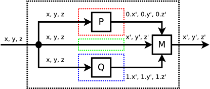
Figure 2: Parallel-by-merge dataflow

The outputs of $P$ and $Q$ are distinguished by a numeral prefix. If $P$ and $Q$ act on an observation space $\mathcal{S}$, then $M$ is a heterogeneous relation of type $[\mathcal{S}\times\mathcal{S}\times\mathcal{S},\mathcal{S}]\textit{{urel}}$, which relates three input copies of $\mathcal{S}$ with a single output $\mathcal{S}$. The merge predicate therefore refers to variables from $P$, using the $0.x$ notation, variables from $Q$, using $1.x$, initial variables, as usual written as $x$, and final variables, as $x^{\prime}$.

A substantial advantage of using parallel-by-merge is that several theorems can be proven for the generic operator. Below, we highlight some of the most important theorems.

Theorem 7.2 (Parallel-by-Merge Laws).

$\displaystyle\left(\bigsqcap_{i\in I}\,P(i)\right)\mathrel{\parallel}_{M}Q$ $\displaystyle=\bigsqcap_{i\in I}\,\left(P(i)\mathrel{\parallel}_{M}Q\right)$ $\displaystyle\hbox{{{{false}}}}\mathrel{\parallel}_{M}P$ $\displaystyle=\hbox{{{{false}}}}$ $\displaystyle P\mathrel{\parallel}_{M}\left(\bigsqcap_{i\in I}\,Q(i)\right)$ $\displaystyle=\bigsqcap_{i\in I}\,\left(P\mathrel{\parallel}_{M}Q(i)\right)$ $\displaystyle P\mathrel{\parallel}_{M}\hbox{{{{false}}}}$ $\displaystyle=\hbox{{{{false}}}}$

$P_{1}\mathrel{\sqsubseteq}P_{2}\mathrel{\wedge}Q_{1}\mathrel{\sqsubseteq}Q_{2}\,\mathrel{\Rightarrow}\,(P_{1}\mathrel{\parallel}_{M}Q_{1})\mathrel{\sqsubseteq}(P_{1}\mathrel{\parallel}_{M}Q_{1})$

Parallel-by-merge distributes through nondeterministic choice ($\bigsqcap$) from both the left and right, regardless of the merge predicate $M$. Since $\bigsqcap$ corresponds to $\mathop{\mathstrut{\exists}}\nolimits$ and also $\vee$, we can similarly distribute through an existential quantification and a disjunction. The miraculous relation false is both a left and right annihilator for parallel composition, which is also monotonic with respect to refinement in both arguments.

Parallel-by-merge may or may not be commutative, depending on the merge predicate. A helpful scheme can be used for proving that parallel composition is commutative, which reduces this to a property of the merge predicate. We adopt a similar approach to [30], but give an account that is more algebraic in nature. We first define the following auxiliary operator.

Definition 7.3 (Merge Swap).

$\hbox{{{{sw}}}}\triangleq\hbox{{{v}}}^{\prime}=\hbox{{{v}}}\mathrel{\wedge}0.\hbox{{{v}}}^{\prime}=1.\hbox{{{v}}}\mathrel{\wedge}1.\hbox{{{v}}}^{\prime}=0.\hbox{{{v}}}$

The relation sw swaps the outputs from the left- and right-hand sides, whilst keeping the initial values (v) the same. Using sw, we can prove the following property of parallel-by-merge.

Theorem 7.4 (Parallel-by-Merge Swap).

$P\mathrel{\parallel}_{\hbox{{{{\small sw}}}}\,\mathrel{\hbox{\rm;}}M}Q=Q\mathrel{\parallel}_{M}P$

This theorem shows that precomposing a merge predicate with sw effectively commutes the arguments $P$ and $Q$. A corollary of this [21], given below, shows how this can be used to demonstrate commutativity.

Theorem 7.5.

$P\mathrel{\parallel}_{M}Q=Q\mathrel{\parallel}_{M}P$ provided that $\hbox{{{{sw}}}}\mathrel{\hbox{\rm;}}M=M$

This theorem shows how proof of commutativity can be reduced to a property of the merge predicate. Specifically, if swapping the order of the inputs to the merge predicate has no effect then it is a symmetric merge, and consequently parallel composition is commutative.

7.2 Parallel Reactive Designs

In previous work [15], we have used parallel-by-merge to prove a general theorem for composing reactive designs. As for the sequential operators, this develops operators that respectively merge the pre-, peri-, and postconditions of the corresponding reactive contract. The theorem below, reproduced from [15], shows how we may calculate a parallel reactive contract using these operators.

Theorem 7.6 (Reactive Design Parallel Composition).

$$\left[\,P_{1}\,\,\scalebox{0.5}[1.0]{$-$}\middle|\,\,\,P_{2}\,\,\middle|\,\,P_{3}\,\right]\mathop{\,{\mathrel{\parallel}}_{\hbox{\tiny\hbox{{{{R}}}}}}^{\text{\tiny$M$}}\,}\left[\,Q_{1}\,\,\scalebox{0.5}[1.0]{$-$}\middle|\,\,\,Q_{2}\,\,\middle|\,\,Q_{3}\,\right]=$$

$$\qquad\left[\,\begin{array}[]{l}(P_{1}\mathop{\mathrel{\Rightarrow}_{\!{r}}}P_{2})\mathop{\,\hbox{{{{wr}}}}_{\text{\tiny$M$}\,}}Q_{1}\mathrel{\wedge}\\ (P_{1}\mathop{\mathrel{\Rightarrow}_{\!{r}}}P_{3})\mathop{\,\hbox{{{{wr}}}}_{\text{\tiny$M$}\,}}Q_{1}\mathrel{\wedge}\\ (Q_{1}\mathop{\mathrel{\Rightarrow}_{\!{r}}}Q_{2})\mathop{\,\hbox{{{{wr}}}}_{\text{\tiny$M$}\,}}P_{1}\mathrel{\wedge}\\ (Q_{1}\mathop{\mathrel{\Rightarrow}_{\!{r}}}Q_{3})\mathop{\,\hbox{{{{wr}}}}_{\text{\tiny$M$}\,}}P_{1}\end{array}\,\,\scalebox{0.5}[1.0]{$-$}\middle|\,\,\,\begin{array}[]{l}P_{2}\mathop{\,{\mathrel{\parallel}}_{\hbox{\tiny\hbox{{{{E}}}}}}^{\text{\tiny M}}\,}Q_{2}\,\mathrel{\vee}\\ P_{3}\mathop{\,{\mathrel{\parallel}}_{\hbox{\tiny\hbox{{{{E}}}}}}^{\text{\tiny M}}\,}Q_{2}\,\mathrel{\vee}\\ P_{2}\mathop{\,{\mathrel{\parallel}}_{\hbox{\tiny\hbox{{{{E}}}}}}^{\text{\tiny M}}\,}Q_{3}\end{array}\,\,\middle|\,\,P_{3}\mathrel{\parallel}_{\text{\tiny M}}Q_{3}\,\right]$$

This complex law describes how the pre-, peri-, and postconditions are merged by the parametric reactive design parallel composition operator $\mathop{\,{\mathrel{\parallel}}_{\hbox{\tiny\hbox{{{{R}}}}}}^{\text{\tiny$M$}}\,}$. Internally, this operator merges the observational variables $ok^{\prime}$ and $wait^{\prime}$ of $P$ and $Q$ using the parallel-by-merge operator and a bespoke merge predicate [15]. Again, as we noted in §4, every NCSP relation corresponds to a reactive contract, and therefore this law applies to any stateful-failure reactive design. Here, $M$ is an “inner merge predicate” [15], which needs to deal only with observational variables like tt, st, and ref; the variables $ok$ and $wait$ having already been merged by $\mathop{\,{\mathrel{\parallel}}_{\hbox{\tiny\hbox{{{{R}}}}}}^{\text{\tiny$M$}}\,}$, which constructs the “outer merge predicate”, to which parallel-by-merge is applied.

The precondition of the composite contract in Theorem 7.6 captures the possible divergent behaviours that both $P$ and $Q$ permit. There are four conjuncts in the precondition, as we require that neither the peri- nor the postcondition can permit divergent behaviour disallowed by its opposing precondition.

The predicate $A\mathop{\,\hbox{{{{wr}}}}_{\text{\tiny$M$}\,}}B$, standing for “weakest rely”, is a reactive condition that describes the weakest context in which reactive relation $A$ does not violate the reactive condition $B$. It is analogous to the reactive weakest precondition operator, $\mathop{\,\hbox{{{{wlp}}}}_{r}\,}$ (outlined in §2.3), but is defined with respect to parallel composition rather than sequential composition. Specifically, whereas $\mathop{\,\hbox{{{{wlp}}}}_{r}\,}$ gives the weakest condition in a sequential context, $\mathop{\,\hbox{{{{wr}}}}_{\text{\tiny$M$}\,}}$ gives the weakest condition in a parallel context. Its definition is given below.

Definition 7.7 (Weakest Rely Condition).

$P\mathop{\,\hbox{{{{wr}}}}_{\text{\tiny$M$}\,}}Q\,\,\triangleq\,\,\neg_{r}\,((\neg_{r}\,Q)\mathrel{\parallel}_{\hbox{\small$M$}\mathrel{\hbox{\rm;}}\hbox{{{{true}}}}_{r}}P)$

This merges the traces that $Q$ does not admit ($\neg_{r}\,Q$) with those of $P$ using the merge predicate $M$ composed with $\hbox{{{{true}}}}_{r}$, which makes $M$ extension closed. It determines all the behaviours permitted by merge predicate $M$ that are enabled by $P$ and yet denied by $Q$. We then negate the overall relation to obtain the reactive precondition. The operator obeys several related laws shown below.

Theorem 7.8 (Weakest Rely Laws).

$$\hbox{{{{false}}}}\mathop{\,\hbox{{{{wr}}}}_{\text{\tiny$M$}\,}}P=\hbox{{{{true}}}}_{r}\qquad P\mathop{\,\hbox{{{{wr}}}}_{\text{\tiny$M$}\,}}\hbox{{{{true}}}}_{r}=\hbox{{{{true}}}}_{r}\qquad\left(\bigvee_{i\in I}\,P(i)\right)\mathop{\,\hbox{{{{wr}}}}_{\text{\tiny$M$}\,}}Q=\left(\bigwedge_{i\in I}\,(P(i)\mathop{\,\hbox{{{{wr}}}}_{\text{\tiny$M$}\,}}Q)\right)$$

The laws show that (1) a miraculous relation satisfies any precondition, (2) any reactive relation satisfies a true precondition, and (3) the weakest rely condition of a disjunction of relations is the conjunction of their weakest rely conditions. These results are similar to those for $\mathop{\,\hbox{{{{wlp}}}}_{r}\,}$

The pericondition in Theorem 7.6 is a disjunction of three terms that calculate possible quiescent merged behaviours. Parallel composition is quiescent when at least one of $P$ and $Q$ is quiescent, and so the three conjuncts characterise quiescence in both, in $Q$ only, and in $P$ only, respectively. The $P\mathop{\,{\mathrel{\parallel}}_{\hbox{\tiny\hbox{{{{E}}}}}}^{\text{\tiny M}}\,}Q\,\,\triangleq\,\,P\mathrel{\parallel}_{\mathop{\mathstrut{\exists}}\nolimits\text{{st}}^{\prime}@M}Q$ operator is an intermediate merge operator, which restricts access to state (see [15, §6.6]). Finally, the overall contract can only terminate when both $P$ and $Q$ do, and so the postcondition simply merges their respective postconditions.

Using these laws, we can show that Miracle is always a annihilator for parallel composition, regardless of the inner merge predicate [15]. The proof exemplifies the calculational approach for parallel composition

Theorem 7.9.

$\hbox{{{{Miracle}}}}\mathop{\,{\mathrel{\parallel}}_{\hbox{\tiny\hbox{{{{R}}}}}}^{\text{\tiny$M$}}\,}P=\hbox{{{{Miracle}}}}$

Proof.

$$\hbox{{{{Miracle}}}}\mathop{\,{\mathrel{\parallel}}_{\hbox{\tiny\hbox{{{{R}}}}}}^{\text{\tiny$M$}}\,}P =\left[\,\hbox{{{{true}}}}_{r}\,\,\scalebox{0.5}[1.0]{$-$}\middle|\,\,\,\hbox{{{{false}}}}\,\,\middle|\,\,\hbox{{{{false}}}}\,\right]\mathop{\,{\mathrel{\parallel}}_{\hbox{\tiny\hbox{{{{R}}}}}}^{\text{\tiny$M$}}\,}\left[\,P_{1}\,\,\scalebox{0.5}[1.0]{$-$}\middle|\,\,\,P_{2}\,\,\middle|\,\,P_{3}\,\right]$$

$$=\left[\,\begin{array}[]{l}(\hbox{{{{true}}}}_{r}\mathop{\mathrel{\Rightarrow}_{\!{r}}}\hbox{{{{false}}}})\mathop{\,\hbox{{{{wr}}}}_{\text{\tiny$M$}\,}}P_{1}\mathrel{\wedge}\\ (\hbox{{{{true}}}}_{r}\mathop{\mathrel{\Rightarrow}_{\!{r}}}\hbox{{{{false}}}})\mathop{\,\hbox{{{{wr}}}}_{\text{\tiny$M$}\,}}P_{1}\mathrel{\wedge}\\ (P_{1}\mathop{\mathrel{\Rightarrow}_{\!{r}}}P_{2})\mathop{\,\hbox{{{{wr}}}}_{\text{\tiny$M$}\,}}\hbox{{{{true}}}}_{r}\mathrel{\wedge}\\ (P_{1}\mathop{\mathrel{\Rightarrow}_{\!{r}}}P_{3})\mathop{\,\hbox{{{{wr}}}}_{\text{\tiny$M$}\,}}\hbox{{{{true}}}}_{r}\end{array}\,\,\scalebox{0.5}[1.0]{$-$}\middle|\,\,\,\begin{array}[]{l}\hbox{{{{false}}}}\mathop{\,{\mathrel{\parallel}}_{\hbox{\tiny\hbox{{{{E}}}}}}^{\text{\tiny M}}\,}P_{2}\,\mathrel{\vee}\\ \hbox{{{{false}}}}\mathop{\,{\mathrel{\parallel}}_{\hbox{\tiny\hbox{{{{E}}}}}}^{\text{\tiny M}}\,}P_{2}\,\mathrel{\vee}\\ \hbox{{{{false}}}}\mathop{\,{\mathrel{\parallel}}_{\hbox{\tiny\hbox{{{{E}}}}}}^{\text{\tiny M}}\,}P_{3}\end{array}\,\,\middle|\,\,\hbox{{{{false}}}}\mathrel{\parallel}_{\text{\tiny M}}P_{3}\,\right] [\ref{thm:rdespar}]$$

$$=\left[\,\begin{array}[]{l}\hbox{{{{false}}}}\mathop{\,\hbox{{{{wr}}}}_{\text{\tiny$M$}\,}}P_{1}\mathrel{\wedge}\hbox{{{{false}}}}\mathop{\,\hbox{{{{wr}}}}_{\text{\tiny$M$}\,}}P_{1}\mathrel{\wedge}\\ \hbox{{{{true}}}}_{r}\mathrel{\wedge}\hbox{{{{true}}}}_{r}\end{array}\,\,\scalebox{0.5}[1.0]{$-$}\middle|\,\,\,\begin{array}[]{l}\hbox{{{{false}}}}\,\mathrel{\vee}\,\hbox{{{{false}}}}\,\mathrel{\vee}\,\hbox{{{{false}}}}\end{array}\,\,\middle|\,\,\hbox{{{{false}}}}\,\right] [\ref{thm:pbm-laws},\ref{thm:wrlaws}]$$

$$=\left[\,\begin{array}[]{l}\hbox{{{{true}}}}_{r}\mathrel{\wedge}\hbox{{{{true}}}}_{r}\end{array}\,\,\scalebox{0.5}[1.0]{$-$}\middle|\,\,\,\begin{array}[]{l}\hbox{{{{false}}}}\end{array}\,\,\middle|\,\,\hbox{{{{false}}}}\,\right] [\ref{thm:wrlaws}]$$

$$=\left[\,\hbox{{{{true}}}}_{r}\,\,\scalebox{0.5}[1.0]{$-$}\middle|\,\,\,\hbox{{{{false}}}}\,\,\middle|\,\,\hbox{{{{false}}}}\,\right]$$

$$=\hbox{{{{Miracle}}}}$$

In this case, the pericondition and the postcondition both reduce to false, since by Theorem 7.2 the merge of any relation with false reduces to false. The four clauses in the precondition all reduce to $\hbox{{{{true}}}}_{r}$ by the weakest rely laws of Theorem 7.8. Thus the entire relation reduces to the Miracle contract. We will next specialise this calculational approach to stateful-failure reactive designs.

7.3 Parallel Stateful-Failure Reactive Designs

Our parallel composition operator is adopted from Circus [39] and has the general form

$$P\mathop{\left|\!\left[ns_{1}\middle|cs\middle|ns_{2}\right]\!\right|}Q$$

for actions $P$ and $Q$, event set $cs\subseteq\textit{Event}$, and name-sets $ns_{1}$ and $ns_{2}$. $P$ and $Q$ both act on the same state space $\mathcal{S}$, and have the same event alphabet (Event). Like for parallel composition in CSP, $P$ and $Q$ must synchronise on events contained in $cs$, but independently engage in events outside $cs$. Since $P$ and $Q$ also have states, we must describe how to merge their final states. We do not permit sharing, and so require partitioning of the state into two independent regions, characterised by two disjoint variable name sets $ns_{1}$ and $ns_{2}$. The final state is then the composition of the two regions. We model these name sets using independent lenses [21] from Isabelle/UTP, that is, $ns_{1}:V_{1}\Longrightarrow\mathcal{S}$, and $ns_{2}:V_{2}\Longrightarrow\mathcal{S}$, for some $V_{1}$ and $V_{2}$ (see §2.2).

As usual [39], we define a few abbreviations for the operator.

Definition 7.10 (Parallel Composition Abbreviations).

$$P\mathop{\left|\!\left[cs\right]\!\right|}Q \triangleq P\mathop{\left|\!\left[\mathbf{0}\middle|cs\middle|\mathbf{0}\right]\!\right|}Q$$

$$P\mathrel{{|}\mkern-2.0mu{|}\mkern-2.0mu{|}}Q \triangleq P\mathop{\left|\!\left[\emptyset\right]\!\right|}Q$$

The operator $P\mathop{\left|\!\left[cs\right]\!\right|}Q$ synchronises on $cs$, but ignores the final state of both $P$ and $Q$. It is therefore broadly equivalent to CSP parallel composition when applied to stateless actions. It uses the special $\mathbf{0}$ lens for the name sets, which characterises an empty region of the state space. The interleaving operator $P\mathrel{{|}\mkern-2.0mu{|}\mkern-2.0mu{|}}Q$ synchronises on none of the events, and requires independent activity for $P$ and $Q$. We denote the general operator using the reactive design parallel-by-merge operator, as shown below.

Definition 7.11 (Parallel Composition).

Let $ns_{1}:\mathcal{V}_{1}\Longrightarrow\mathcal{S}$ and $ns_{2}:\mathcal{V}_{2}\Longrightarrow\mathcal{S}$ be lenses that characterise disjoint regions, $\mathcal{V}_{1}$ and $\mathcal{V}_{2}$, of the state space $\mathcal{S}$ (that is, $ns_{1}\mathop{\,\bowtie\,}ns_{2}$), and let $cs$ be a set of events. Parallel composition is then defined as follows:

$$P\mathop{\left|\!\left[ns_{1}\middle|cs\middle|ns_{2}\right]\!\right|}Q \triangleq P\mathop{\,{\mathrel{\parallel}}_{\hbox{\tiny\hbox{{{{R}}}}}}^{\text{\tiny$N_{\textsf{\tiny C}}$}}\,}Q$$

$$\text{where}\,N_{\textsf{\tiny C}}{\scriptsize\begin{bmatrix}ns_{1}\\ cs\\ ns_{2}\end{bmatrix}} \triangleq\left(\begin{array}[]{l}\text{{tt}}\in 0.\text{{tt}}\mathrel{\parallel}_{cs}1.\text{{tt}}\\ \mathrel{\wedge}0.\text{{tt}}\mathrel{\upharpoonright}cs=1.\text{{tt}}\mathrel{\upharpoonright}cs\\ \mathrel{\wedge}\text{{ref}}^{\prime}\subseteq((0.\text{{ref}}\cup 1.\text{{ref}})\cap cs)\cup((0.\text{{ref}}\cap 1.\text{{ref}})\setminus cs)\\ \mathrel{\wedge}\text{{st}}^{\prime}=\text{{st}}\lhd_{ns_{1}}0.\text{{st}}\lhd_{ns_{2}}1.\text{{st}}\end{array}\right)$$

Here, $N_{\textsf{\tiny C}}$ is an inner merge predicate [15] with arguments $ns_{1}$, $cs$, and $ns_{2}$, which we omit when they can be determined from the context. It defines how the traces, states, and refusal sets from $P$ and $Q$ are merged. It is adapted from the original Circus merge predicate [40, 39], which also defines the function $t_{1}\mathrel{\parallel}_{cs}t_{2}$ that specifies the set of traces obtained by merging traces $t_{1}$ and $t_{2}$, synchronising on the events in $cs$. For completeness, we define this recursive function below, adapting slightly the original definition [40].

Definition 7.12 (Trace Merge Function).

We define $\mathrel{\parallel}_{cs}:\mathop{\mathrm{seq}}E\to\mathop{\mathrm{seq}}E\to\mathop{\mathstrut{\mathbb{P}}}\nolimits(\mathop{\mathrm{seq}}\,E)$ to be the least function that satisfies the following equations:

$$\langle\rangle\mathrel{\parallel}_{cs}\langle\rangle =\{\langle\rangle\}$$

$$(e\mathop{::}t)\mathrel{\parallel}_{cs}\langle\rangle =\left(\{\langle\rangle\}\mathop{\hbox{\raisebox{0.0pt}{$\triangleleft$}}}e\in cs\mathop{\hbox{\raisebox{0.0pt}{$\triangleright$}}}\left(\{\langle e\rangle\}\frown(t\mathrel{\parallel}_{cs}\langle\rangle)\right)\right)$$

$$\langle\rangle\mathrel{\parallel}_{cs}(e\mathop{::}t) =\left(\{\langle\rangle\}\mathop{\hbox{\raisebox{0.0pt}{$\triangleleft$}}}e\in cs\mathop{\hbox{\raisebox{0.0pt}{$\triangleright$}}}\left(\{\langle e\rangle\}\frown(\langle\rangle\mathrel{\parallel}_{cs}t)\right)\right)$$

$$(e\mathop{::}t_{1})\mathrel{\parallel}_{cs}(e\mathop{::}t_{2}) =(\langle e\rangle\frown(t_{1}\mathrel{\parallel}_{cs}t_{2}))\mathop{\hbox{\raisebox{0.0pt}{$\triangleleft$}}}e\in cs\mathop{\hbox{\raisebox{0.0pt}{$\triangleright$}}}\left(\{\langle e\rangle\}\frown(t_{1}\mathrel{\parallel}_{cs}(e\mathop{::}t_{2})\cup(e\mathop{::}t_{1})\mathrel{\parallel}_{cs}t_{2})\right)$$

$$(e_{1}\mathop{::}t_{1})\mathrel{\parallel}_{cs}(e_{2}\mathop{::}t_{2}) =\left(\begin{array}[]{l}\left(\{\langle\rangle\}\mathop{\hbox{\raisebox{0.0pt}{$\triangleleft$}}}e_{2}\in cs\mathop{\hbox{\raisebox{0.0pt}{$\triangleright$}}}\left(\{\langle e_{2}\rangle\}\frown((e_{1}\mathop{::}t_{1})\mathrel{\parallel}_{cs}t_{2})\right)\right)\\ \quad\mathop{\hbox{\raisebox{0.0pt}{$\triangleleft$}}}e_{1}\in cs\mathop{\hbox{\raisebox{0.0pt}{$\triangleright$}}}\\ \left(\begin{array}[]{l}\left(\{\langle e_{1}\rangle\}\frown(t_{1}\mathrel{\parallel}_{cs}(e_{2}\mathop{::}t_{2}))\right)\\ \quad\mathop{\hbox{\raisebox{0.0pt}{$\triangleleft$}}}e_{2}\in cs\mathop{\hbox{\raisebox{0.0pt}{$\triangleright$}}}\\ \left((\{\langle e_{1}\rangle\}\frown(t_{1}\mathrel{\parallel}_{cs}(e_{2}\mathop{::}t_{2})))\cup(\{\langle e_{2}\rangle\}\frown((e_{1}\mathop{::}t_{1})\mathrel{\parallel}_{cs}t_{2}))\right)\end{array}\right)\end{array}\right) e_{1}\neq e_{2}$$

where $ts_{1}\frown ts_{2}\triangleq\left\{t_{1}\mathbin{\smash{\raise 3.44444pt\hbox{$\smallfrown$}}}t_{2}|t_{1}\in ts_{1}\mathrel{\wedge}t_{2}\in ts_{2}\right\}$

Here, the operator $x\mathop{::}xs$ constructs a sequence by composing an element $x$ with an existing sequence $xs$. The trace merge function $t_{1}\mathrel{\parallel}_{cs}t_{2}$ produces the set of maximal possible merges from every pair of traces; that is the traces that include the maximum possible number of events from both $t_{1}$ and $t_{2}$, ordered to reflect synchronisation on th events in $cs$ [40]. If an event is encountered in $cs$, then both traces must agree to allow this event simultaneously for behaviour to progress. For any other events, all possible interleavings are recorded.

The merge predicate $N_{\textsf{\tiny C}}$ in Definition 7.11 has four conjuncts. The first conjunct states that any permissible trace tt arises from merging the constituent traces $0.\text{{tt}}$ and $1.\text{{tt}}$. The second ensures that the same synchronisations on events from $cs$ occur in both $0.\text{{tt}}$ and $1.\text{{tt}}$ in the same order. Filter function $t\mathrel{\upharpoonright}cs$ returns the elements of sequence $t$ that are contained in $cs$, whilst retaining the order and number of occurrences. A consequence of the second conjunct is that the resulting trace contains, in a suitable order, all the events from both constituents. The third conjunct requires that the overall refusal is either a subset of the set of synchronised events independently refused ($(0.\text{{ref}}\cup 1.\text{{ref}})\cap cs$), or the non-synchronised events refused by both ($(0.\text{{ref}}\cap 1.\text{{ref}})\setminus cs$). The fourth conjunct constructs the final state by merging the $ns_{1}$ region of $P$’s state, the $ns_{2}$ region of $Q$’s state, and the remaining region from the initial state. It uses the lens override operator $s_{1}\lhd_{ns}s_{2}$ from Definition 2.6.

The parallel operator of Definition 7.11 is not, in general, commutative due to its asymmetric partitioning of the state space. However, we can prove a useful theorem of the inner merge predicate.

Theorem 7.13 (Swap Inner Merge).

If $ns_{1}\mathop{\,\bowtie\,}ns_{2}$ then $\hbox{{{{sw}}}}\mathrel{\hbox{\rm;}}N_{\textsf{\tiny C}}{\scriptsize\begin{bmatrix}ns_{1}\\ cs\\ ns_{2}\end{bmatrix}}=N_{\textsf{\tiny C}}{\scriptsize\begin{bmatrix}ns_{2}\\ cs\\ ns_{1}\end{bmatrix}}$

If we precompose $N_{\textsf{\tiny C}}$ with the swap relation (sw), then this amounts to switching the name sets. The proof of this depends on the commutativity of $\mathrel{\parallel}_{cs}$, a property that is proved in [39], and on Theorem 2.7 to switch the name set lenses. A corollary of Theorem 7.13 is a quasi-commutativity theorem for our parallel composition operator.

Theorem 7.14.

If $ns_{1}\mathop{\,\bowtie\,}ns_{2}$ then $P\mathop{\left|\!\left[ns_{1}\middle|cs\middle|ns_{2}\right]\!\right|}Q=Q\mathop{\left|\!\left[ns_{2}\middle|cs\middle|ns_{1}\right]\!\right|}P$

Thus, we can commute a parallel composition by also commuting the respective name sets.

7.4 Composing Reactive Relations

In order to calculate a stateful-failure reactive design for parallel composition, we specialise Theorem 7.6. This requires that we have specialised versions of the merge operators for peri- and postconditions, and also a specialised weakest rely condition operator. These are defined below.

Definition 7.15 (Intermediate Merge, Final Merge, and Weakest Rely Condition).

$$\textstyle P\mathop{\textstyle\mathop{\left|\!\left[cs\right]\!\right|}_{\mbox{\tiny{{I}}}}\,}Q \triangleq P\mathrel{\parallel}_{(\mathop{\mathstrut{\exists}}\nolimits\text{{st}}^{\prime}@N_{\textsf{\tiny I}})}Q$$

$$\textstyle P\mathop{\textstyle\mathop{\left|\!\left[ns_{1}\middle|cs\middle|ns_{2}\right]\!\right|}_{\mbox{\tiny{{F}}}}\,}Q \triangleq P\mathrel{\parallel}_{(\mathop{\mathstrut{\exists}}\nolimits\text{{ref}}^{\prime}@N_{\textsf{\tiny C}})}Q$$

$$P\mathop{\,\hbox{{{{wr}}}}\!\left[cs\right]\,}Q \triangleq P\mathop{\,\hbox{{{{wr}}}}_{\text{\tiny$N_{\textsf{\tiny I}}$}\,}}Q$$

where $N_{\textsf{\tiny I}}\triangleq N_{\textsf{\tiny C}}{\scriptsize\begin{bmatrix}\mathbf{0}\\ cs\\ \mathbf{0}\end{bmatrix}}$

The intermediate merge, $\mathop{\textstyle\mathop{\left|\!\left[cs\right]\!\right|}_{\mbox{\tiny{{I}}}}\,}$ defines how two quiescent observations are merged. It is parametrised only in $cs$ and not $ns_{1}$ or $ns_{2}$, as state is concealed in quiescent observations. Its definition applies the merge predicate $(\mathop{\mathstrut{\exists}}\nolimits\text{{st}}^{\prime}@N_{\textsf{\tiny I}})$, which abstracts from the final state and is defined in terms of $N_{\textsf{\tiny I}}$. The latter applies $N_{\textsf{\tiny C}}$, but uses the $\mathbf{0}$ lens for $ns_{1}$ and $ns_{2}$, and therefore ignores the final state of $P$ and $Q$.

The final state merge $\mathop{\textstyle\mathop{\left|\!\left[ns_{1}\middle|cs\middle|ns_{2}\right]\!\right|}_{\mbox{\tiny{{F}}}}\,}$ defines how terminated observations are merged. It is defined similarly, but abstracts from $\text{{ref}}^{\prime}$, since there is no refusal information in a final observation, and uses $N_{\textsf{\tiny C}}$ directly to merge the states. Finally, the weakest rely condition $\mathop{\,\hbox{{{{wr}}}}\!\left[cs\right]\,}$ is simply the general reactive design version, using $N_{\textsf{\tiny I}}$ as the merge predicate as final states are also not relevant in preconditions.

We now demonstrate the healthiness of these new operators.

Theorem 7.16 (Merge Closure Properties).

1. If $P$ and $Q$ are CRR-healthy then $P\mathop{\textstyle\mathop{\left|\!\left[cs\right]\!\right|}_{\mbox{\tiny{{I}}}}\,}Q$ is CRR-healthy.

2. $P\mathop{\textstyle\mathop{\left|\!\left[cs\right]\!\right|}_{\mbox{\tiny{{I}}}}\,}Q$ does not refer to $\text{{st}}^{\prime}$.

3. If $P$ and $Q$ are CRF-healthy then $P\mathop{\textstyle\mathop{\left|\!\left[ns_{1}\middle|cs\middle|ns_{2}\right]\!\right|}_{\mbox{\tiny{{F}}}}\,}Q$ is CRF-healthy.

4. If $P$ is CRR-healthy and $Q$ is CRC-healthy, then $P\mathop{\,\hbox{{{{wr}}}}\!\left[cs\right]\,}Q$ is CRC-healthy.

The intermediate merge constructs a reactive relation that does not refer to the final state. The final merge constructs a reactive finaliser, since it does not refer to $\text{{ref}}^{\prime}$. Weakest rely constructs a reactive condition. Following a similar approach to Theorem 7.14, we can also demonstrate commutativity properties.

Theorem 7.17 (Inner Merge Commutativity).

$$P\mathop{\textstyle\mathop{\left|\!\left[cs\right]\!\right|}_{\mbox{\tiny{{I}}}}\,}Q =Q\mathop{\textstyle\mathop{\left|\!\left[cs\right]\!\right|}_{\mbox{\tiny{{I}}}}\,}P$$

$$P\mathop{\textstyle\mathop{\left|\!\left[ns_{1}\middle|cs\middle|ns_{2}\right]\!\right|}_{\mbox{\tiny{{F}}}}\,}Q =Q\mathop{\textstyle\mathop{\left|\!\left[ns_{2}\middle|cs\middle|ns_{1}\right]\!\right|}_{\mbox{\tiny{{F}}}}\,}P ns_{1}\mathop{\,\bowtie\,}ns_{2}$$

Using these new operators, we can finally prove the specialised calculation law for parallel composition.

Theorem 7.18 (Parallel Calculation).

$$\left[\,P_{1}\,\,\scalebox{0.5}[1.0]{$-$}\middle|\,\,\,P_{2}\,\,\middle|\,\,P_{3}\,\right]\mathop{\left|\!\left[ns_{1}\middle|cs\middle|ns_{2}\right]\!\right|}\left[\,Q_{1}\,\,\scalebox{0.5}[1.0]{$-$}\middle|\,\,\,Q_{2}\,\,\middle|\,\,Q_{3}\,\right]=$$

$$\qquad\left[\,\begin{array}[]{l}(P_{1}\mathop{\mathrel{\Rightarrow}_{\!{r}}}P_{2})\mathop{\,\hbox{{{{wr}}}}\!\left[cs\right]\,}Q_{1}\mathrel{\wedge}\\ (P_{1}\mathop{\mathrel{\Rightarrow}_{\!{r}}}P_{3})\mathop{\,\hbox{{{{wr}}}}\!\left[cs\right]\,}Q_{1}\mathrel{\wedge}\\ (Q_{1}\mathop{\mathrel{\Rightarrow}_{\!{r}}}Q_{2})\mathop{\,\hbox{{{{wr}}}}\!\left[cs\right]\,}P_{1}\mathrel{\wedge}\\ (Q_{1}\mathop{\mathrel{\Rightarrow}_{\!{r}}}Q_{3})\mathop{\,\hbox{{{{wr}}}}\!\left[cs\right]\,}P_{1}\end{array}\,\,\scalebox{0.5}[1.0]{$-$}\middle|\,\,\,\begin{array}[]{l}P_{2}\mathop{\textstyle\mathop{\left|\!\left[cs\right]\!\right|}_{\mbox{\tiny{{I}}}}\,}Q_{2}\,\,\mathrel{\vee}\\ P_{3}\mathop{\textstyle\mathop{\left|\!\left[cs\right]\!\right|}_{\mbox{\tiny{{I}}}}\,}Q_{2}\,\,\mathrel{\vee}\\ P_{2}\mathop{\textstyle\mathop{\left|\!\left[cs\right]\!\right|}_{\mbox{\tiny{{I}}}}\,}Q_{3}\end{array}\,\,\middle|\,\,\textstyle P_{3}\mathop{\textstyle\mathop{\left|\!\left[ns_{1}\middle|cs\middle|ns_{2}\right]\!\right|}_{\mbox{\tiny{{F}}}}\,}Q_{3}\,\right]$$

This is similar to Theorem 7.6, but uses the specialised merge and weakest rely operators. This theorem shows that calculation of reactive contracts can be reduced to merging the peri- and postconditions. A corollary, for the simpler case when the preconditions are both $\hbox{{{{true}}}}_{r}$, is given below.

Theorem 7.19 (Simplified Parallel Calculation).

$$\left[\,\!\,\,\scalebox{0.5}[1.0]{$-$}\middle|\,\,\,P_{2}\,\,\middle|\,\,P_{3}\,\right]\mathop{\left|\!\left[ns_{1}\middle|cs\middle|ns_{2}\right]\!\right|}\left[\,\!\,\,\scalebox{0.5}[1.0]{$-$}\middle|\,\,\,Q_{2}\,\,\middle|\,\,Q_{3}\,\right]=\left[\,\!\,\,\scalebox{0.5}[1.0]{$-$}\middle|\,\,\,P_{2}\mathop{\textstyle\mathop{\left|\!\left[cs\right]\!\right|}_{\mbox{\tiny{{I}}}}\,}Q_{2}\mathrel{\vee}P_{3}\mathop{\textstyle\mathop{\left|\!\left[cs\right]\!\right|}_{\mbox{\tiny{{I}}}}\,}Q_{2}\mathrel{\vee}P_{2}\mathop{\textstyle\mathop{\left|\!\left[cs\right]\!\right|}_{\mbox{\tiny{{I}}}}\,}Q_{3}\,\,\middle|\,\,P_{3}\mathop{\textstyle\mathop{\left|\!\left[ns_{1}\middle|cs\middle|ns_{2}\right]\!\right|}_{\mbox{\tiny{{F}}}}\,}Q_{3}\,\right]$$

This follows by application of Theorem 7.8 because $P\mathop{\,\hbox{{{{wr}}}}\!\left[cs\right]\,}\hbox{{{{true}}}}_{r}=\hbox{{{{true}}}}_{r}$. We can also show, with the help of Theorems 4.3 and 7.16, that NCSP is closed under parallel composition.

Theorem 7.20.

If $P$ and $Q$ are NCSP-healthy, and $ns_{1}\mathop{\,\bowtie\,}ns_{2}$, then $P\mathop{\left|\!\left[ns_{1}\middle|cs\middle|ns_{2}\right]\!\right|}Q$ is NCSP-healthy.

For sequential processes, we have already shown that the peri- and postconditions of reactive programs can be specified using disjunctions of the $\mathcal{E}$ and $\Phi$ operators. Consequently, to extend our calculational method to parallel composition, we need to prove how these operators should be merged. The following theorems show how reactive relations describing final and intermediate observations are merged.

Theorem 7.21 (Merging Finalisers).

If $ns_{1}\mathop{\,\bowtie\,}ns_{2}$ then

$$\Phi\!\left[s_{1},\sigma_{1},t_{1}\right]\,\mathop{\textstyle\mathop{\left|\!\left[ns_{1}\middle|cs\middle|ns_{2}\right]\!\right|}_{\mbox{\tiny{{F}}}}\,}\,\Phi\!\left[s_{2},\sigma_{2},t_{2}\right] =\left(\mathop{\mathstrut{\exists}}\nolimits t@\Phi\!\left[s_{1}\mathrel{\wedge}s_{2}\mathrel{\wedge}t\in t_{1}\!\mathrel{\parallel}_{cs}\!t_{2}\mathrel{\wedge}t_{1}\mathrel{\upharpoonright}cs=t_{2}\mathrel{\upharpoonright}cs,\sigma_{1}\mathop{\left[ns_{1}\middle|ns_{2}\right]\,}\sigma_{2},t\right]\right)$$

$$\Phi\!\left[s_{1},\sigma_{1},\langle\rangle\right]\,\mathop{\textstyle\mathop{\left|\!\left[ns_{1}\middle|cs\middle|ns_{2}\right]\!\right|}_{\mbox{\tiny{{F}}}}\,}\,\Phi\!\left[s_{2},\sigma_{2},\langle\rangle\right] =\Phi\!\left[s_{1}\mathrel{\wedge}s_{2},\sigma_{1}\mathop{\left[ns_{1}\middle|ns_{2}\right]\,}\sigma_{2},\langle\rangle\right]$$

The first equation shows how to merge two finalisers. We require the existence of the trace $t$, which is one of the possible merges of $t_{1}$ and $t_{2}$, and require that both preconditions $s_{1}$ and $s_{2}$ hold initially. The overall trace of the finaliser is then $t$. The second equation is a corollary for when both traces are empty, and the event merge is trivial. In either case, the final state update is constructed using the operator $\mathop{\left[ns_{1}\middle|ns_{2}\right]\,}$, which uses lens override to merge the two disjoint state updates. It obeys the following laws.

Theorem 7.22.

Given independent lenses, $ns_{1}\mathop{\,\bowtie\,}ns_{2}$, the following identities hold:

$$id\mathop{\left[ns_{1}\middle|ns_{2}\right]\,}id =id$$ (1)

$$\sigma\mathop{\left[ns_{1}\middle|ns_{2}\right]\,}\rho =\rho\mathop{\left[ns_{2}\middle|ns_{1}\right]\,}\sigma$$ (2)

$$(\sigma(x\mapsto v))\mathop{\left[ns_{1}\middle|ns_{2}\right]\,}\rho =(\sigma\mathop{\left[ns_{1}\middle|ns_{2}\right]\,}\rho)(x\mapsto v) x\preceq ns_{1}$$ (3)

$$(\sigma(x\mapsto v))\mathop{\left[ns_{1}\middle|ns_{2}\right]\,}\rho =\sigma\mathop{\left[ns_{1}\middle|ns_{2}\right]\,}\rho x\mathop{\,\bowtie\,}ns_{1}$$ (4)

Merging two identity (vacuous) assignments yields an identity assignment (1). The operator is quasi-commutative, when the name sets are also swapped (2). When one of the assignments is constructed with a state update, if the variable being assigned is part of the corresponding name set ($x\preceq ns_{1}$), then the update is applied to the top-level assignment (3). Effectively, this means that the assignment is retained when the parallel composition terminates. Conversely, if the assignment is to a variable outside of the name set ($x\mathop{\,\bowtie\,}ns_{1}$), then its effect is lost (4). Using these laws we calculate the contracts for some examples.

Example 7.23.

We assume the existence of lenses $x$ and $y$, with $x\preceq ns_{1}$, $y\preceq ns_{2}$, and $ns_{1}\mathop{\,\bowtie\,}ns_{2}$, and calculate the meaning of parallel assignment to these variables.

$$(x:=u)\mathop{\left|\!\left[ns_{1}\middle|cs\middle|ns_{2}\right]\!\right|}(y:=v)$$

$$=\, \left[\,\!\,\,\scalebox{0.5}[1.0]{$-$}\middle|\,\,\,\hbox{{{{false}}}}\,\,\middle|\,\,\Phi\!\left[\llparenthesis x\mapsto u\rrparenthesis,\langle\rangle\right]\,\right]\mathop{\left|\!\left[ns_{1}\middle|cs\middle|ns_{2}\right]\!\right|}\left[\,\!\,\,\scalebox{0.5}[1.0]{$-$}\middle|\,\,\,\hbox{{{{false}}}}\,\,\middle|\,\,\Phi\!\left[\llparenthesis y\mapsto v\rrparenthesis,\langle\rangle\right]\,\right] [\ref{thm:bcircus-def}]$$

$$=\, \left[\,\!\,\,\scalebox{0.5}[1.0]{$-$}\middle|\,\,\,\begin{array}[]{l}\hbox{{{{false}}}}\,\mathop{\textstyle\mathop{\left|\!\left[cs\right]\!\right|}_{\mbox{\tiny{{I}}}}\,}\,\hbox{{{{false}}}}\\ \mathrel{\vee}\Phi\!\left[\llparenthesis x\mapsto u\rrparenthesis,\langle\rangle\right]\,\mathop{\textstyle\mathop{\left|\!\left[cs\right]\!\right|}_{\mbox{\tiny{{I}}}}\,}\,\hbox{{{{false}}}}\\ \mathrel{\vee}\hbox{{{{false}}}}\,\mathop{\textstyle\mathop{\left|\!\left[cs\right]\!\right|}_{\mbox{\tiny{{I}}}}\,}\Phi\!\left[\llparenthesis y\mapsto v\rrparenthesis,\langle\rangle\right]\end{array}\,\,\middle|\,\,\Phi\!\left[\llparenthesis x\mapsto u\rrparenthesis,\langle\rangle\right]\mathop{\textstyle\mathop{\left|\!\left[ns_{1}\middle|cs\middle|ns_{2}\right]\!\right|}_{\mbox{\tiny{{F}}}}\,}\Phi\!\left[\llparenthesis y\mapsto v\rrparenthesis,\langle\rangle\right]\,\right] [\ref{thm:snrdespar}]$$

$$=\, \left[\,\!\,\,\scalebox{0.5}[1.0]{$-$}\middle|\,\,\,\hbox{{{{false}}}}\,\,\middle|\,\,\Phi\!\left[\llparenthesis x\mapsto u\rrparenthesis\,\mathop{\left[ns_{1}\middle|ns_{2}\right]\,}\,\llparenthesis y\mapsto v\rrparenthesis,\langle\rangle\right]\,\right] [\ref{thm:pbm-laws},\ref{thm:rrmerge}]$$

$$=\, \left[\,\!\,\,\scalebox{0.5}[1.0]{$-$}\middle|\,\,\,\hbox{{{{false}}}}\,\,\middle|\,\,\Phi\!\left[\llparenthesis x\mapsto u,y\mapsto v\rrparenthesis,\langle\rangle\right]\,\right] [\ref{thm:subpar}]$$

$$=\, \langle x\mapsto u,y\mapsto v\rangle_{\hbox{\tiny\hbox{{{{C}}}}}} [\ref{thm:bcircus-def}]$$

This does not rule out having $u\triangleq y$ and $v\triangleq x$, since both processes have access to the entirety of the initial state. We first calculate the contract for the two assignments. Since the preconditions are trivial, we apply Theorem 7.19 to compute the composition contract. Since both periconditions are false, by application of Theorem 7.2 and relational calculus, the overall pericondition is also false. Thus, we can simply apply Theorem 7.21 to compute the merge of the two finalisers, and then Theorem 7.22 to merge the two assignments. The final form is, by Definition 4.7, equivalent to a single assignment. In Isabelle/UTP, this proof of this equality is fully automated by the rdes-eq tactic [15].

Using a similar calculation, and using Definition 7.10, we can also show that

$$(x:=u)\mathrel{{|}\mkern-2.0mu{|}\mkern-2.0mu{|}}(y:=v)=\hbox{{{{Skip}}}}$$

The name sets are both $\mathbf{0}$ and consequently, since $x\mathop{\,\bowtie\,}\mathbf{0}$ and $y\mathop{\,\bowtie\,}\mathbf{0}$, both assignments are lost. ∎

The independence constraints on the process state spaces and loss of assignments may, at first sight, seem unsatisfactory as this prevents shared variables. However, variables here are only for the sequential case. Shared variables in languages like CSP and Circus should be modelled using channel communication, for separation of concerns. This approach has been demonstrated in several previous works [43], including JCSP [51] and the RoboChart state-machine language [36].

We next show how quiescent observations are merged using the $\mathop{\textstyle\mathop{\left|\!\left[cs\right]\!\right|}_{\mbox{\tiny{{I}}}}\,}$.

Theorem 7.24 (Merging Quiescent Observations).

$$\mathcal{E}\!\left[s_{1},t_{1},E_{1}\right]\,\mathop{\textstyle\mathop{\left|\!\left[cs\right]\!\right|}_{\mbox{\tiny{{I}}}}\,}\,\mathcal{E}\!\left[s_{2},t_{2},E_{2}\right] =\left(\mathop{\mathstrut{\exists}}\nolimits t@\mathcal{E}\!\left[\left(\begin{array}[]{l}s_{1}\mathrel{\wedge}s_{2}\mathrel{\wedge}t\in t_{1}\!\mathrel{\parallel}_{cs}\!t_{2}\mathrel{\wedge}\\ t_{1}\mathrel{\upharpoonright}cs=t_{2}\mathrel{\upharpoonright}cs\end{array}\right),t,\left(\!\begin{array}[]{l}(E_{1}\cap E_{2}\cap cs)\,\cup\\ ((E_{1}\cup E_{2})\setminus cs)\end{array}\!\right)\right]\right)$$

$$\mathcal{E}\!\left[s_{1},t_{1},E_{1}\right]\,\mathop{\textstyle\mathop{\left|\!\left[cs\right]\!\right|}_{\mbox{\tiny{{I}}}}\,}\,\Phi\!\left[s_{2},\sigma_{2},t_{2}\right] =\left(\mathop{\mathstrut{\exists}}\nolimits t@\mathcal{E}\!\left[\left(\begin{array}[]{l}s_{1}\mathrel{\wedge}s_{2}\mathrel{\wedge}t\in t_{1}\!\mathrel{\parallel}_{cs}\!t_{2}\mathrel{\wedge}\\ t_{1}\mathrel{\upharpoonright}cs=t_{2}\mathrel{\upharpoonright}cs\end{array}\right),t,E_{1}\setminus cs\right]\right)$$

The equations in Theorem 7.24 are similar to those in Theorem 7.21, but involve at least one quiescent observation. We omit the symmetric case, since we know that $\mathop{\textstyle\mathop{\left|\!\left[cs\right]\!\right|}_{\mbox{\tiny{{I}}}}\,}$ is commutative. As for the finaliser, we need to merge the traces $t_{1}$ and $t_{2}$. There is no state update merge, as this is a quiescent observation. We also need to consider merging the refusal sets together, which here are given by a set of accepted events. If merging two quiescent observations, we accept (1) the events in the synchronisation set $cs$ enabled by both $P$ and $Q$ ($E_{1}\cap E_{2}\cap cs$); and (2) the events not in $cs$ that enabled available in either $P$ or $Q$ ($(E_{1}\cup E_{2})\setminus cs$). If a quiescent observation is merged with a final observation, then the accepted events are simply those not in $cs$, that is $E_{1}\setminus cs$.

In order to illustrate the use of these theorems, we provide the following example.

Example 7.25.

We calculate the meaning of $a\mathrel{\rightarrow}b\mathrel{\rightarrow}\hbox{{{{Skip}}}}\mathop{\left|\!\left[\{b\}\right]\!\right|}b\mathrel{\rightarrow}c\mathrel{\rightarrow}\hbox{{{{Skip}}}}$.

$$=\, \left.\left[\,\,\,\scalebox{0.5}[1.0]{$-$}\middle|\,\,\,\begin{array}[]{l}\mathcal{E}\!\left[\langle\rangle,\{a\}\right]\mathrel{\vee}\\ \mathcal{E}\!\left[\langle a\rangle,\{b\}\right]\end{array}\,\,\middle|\,\,\Phi\!\left[id,\langle a,b\rangle\right]\,\right]\,\middle|\!\middle[\{b\}\middle]\!\middle|\,\left[\,\,\,\scalebox{0.5}[1.0]{$-$}\middle|\,\,\,\begin{array}[]{l}\mathcal{E}\!\left[\langle\rangle,\{b\}\right]\mathrel{\vee}\\ \mathcal{E}\!\left[\langle b\rangle,\{c\}\right]\end{array}\,\,\middle|\,\,\Phi\!\left[id,\langle b,c\rangle\right]\,\right]\right.$$ (5)

$$=\, \left[\,\,\,\scalebox{0.5}[1.0]{$-$}\middle|\,\,\,\begin{array}[]{l}\mathcal{E}\!\left[\langle\rangle,\{a\}\right]\,\mathop{\textstyle\mathop{\left|\!\left[\{b\}\right]\!\right|}_{\mbox{\tiny{{I}}}}\,}\,\mathcal{E}\!\left[\langle\rangle,\{b\}\right]\mathrel{\vee}\\ \mathcal{E}\!\left[\langle\rangle,\{a\}\right]\,\mathop{\textstyle\mathop{\left|\!\left[\{b\}\right]\!\right|}_{\mbox{\tiny{{I}}}}\,}\,\mathcal{E}\!\left[\langle b\rangle,\{c\}\right]\mathrel{\vee}\\ \mathcal{E}\!\left[\langle\rangle,\{a\}\right]\,\mathop{\textstyle\mathop{\left|\!\left[\{b\}\right]\!\right|}_{\mbox{\tiny{{I}}}}\,}\,\Phi\!\left[id,\langle b,c\rangle\right]\mathrel{\vee}\\ \mathcal{E}\!\left[\langle a\rangle,\{b\}\right]\,\mathop{\textstyle\mathop{\left|\!\left[\{b\}\right]\!\right|}_{\mbox{\tiny{{I}}}}\,}\,\mathcal{E}\!\left[\langle\rangle,\{b\}\right]\mathrel{\vee}\\ \mathcal{E}\!\left[\langle a\rangle,\{b\}\right]\,\mathop{\textstyle\mathop{\left|\!\left[\{b\}\right]\!\right|}_{\mbox{\tiny{{I}}}}\,}\,\mathcal{E}\!\left[\langle b\rangle,\{c\}\right]\mathrel{\vee}\\ \cdots\end{array}\,\,\middle|\,\,\Phi\!\left[id,\langle a,b\rangle\right]\,\mathop{\textstyle\mathop{\left|\!\left[\mathbf{0}\middle|\{b\}\middle|\mathbf{0}\right]\!\right|}_{\mbox{\tiny{{F}}}}\,}\,\Phi\!\left[id,\langle b,c\rangle\right]\,\right]$$ (12)

$$=\, \left[\,\,\,\scalebox{0.5}[1.0]{$-$}\middle|\,\,\,\!\begin{array}[]{l}\left(\!\mathop{\mathstrut{\exists}}\nolimits t@\mathcal{E}\!\left[\left(\begin{array}[]{l}t\in\langle\rangle\!\mathrel{\parallel}_{\{\!b\}}\!\langle\rangle\mathrel{\wedge}\\ \langle\rangle\!\mathrel{\upharpoonright}\!cs=\langle\rangle\!\mathrel{\upharpoonright}\!cs\end{array}\!\right),t,\!\!\begin{array}[]{l}\{a\}\!\cap\!\{b\}\!\cap\!\{b\}\cup\\ (\{a\}\!\cup\!\{b\})\setminus\{b\}\end{array}\!\right]\right)\\ \,\mathrel{\vee}\cdots\end{array}\!\!\,\,\middle|\,\,\mathop{\mathstrut{\exists}}\nolimits t@\Phi\!\left[\begin{array}[]{l}t\in\langle a,b\rangle\mathrel{\parallel}_{\{b\}}\langle b,c\rangle\mathrel{\wedge}\\ \langle a,b\rangle\mathrel{\upharpoonright}\{b\}=\langle b,c\rangle\mathrel{\upharpoonright}\{b\}\end{array},id,t\right]\,\right]$$ (21)

$$=\, \left[\,\,\,\scalebox{0.5}[1.0]{$-$}\middle|\,\,\,\mathcal{E}\!\left[\langle\rangle,\{a\}\right]\mathrel{\vee}\mathcal{E}\!\left[\langle a\rangle,\{b\}\right]\mathrel{\vee}\mathcal{E}\!\left[\langle a,b\rangle,\{c\}\right]\,\,\middle|\,\,\Phi\!\left[id,\langle a,b,c\rangle\right]\,\right]$$ (22)

$$=\, a\mathrel{\rightarrow}b\mathrel{\rightarrow}c\mathrel{\rightarrow}\hbox{{{{Skip}}}}$$ (23)

Step (5) calculates the sequential contracts for the left- and right-hand sides of the parallel composition using the rules already outlined in §4. Step (12) expands out all the possible merges for the peri- and postcondition, by application of Theorem 7.18, and also Theorem 7.2 to distribute through the various disjunctions. There are a total of nine observations (of which we show five) in the pericondition, because we need to merge every disjunct of the pericondition, plus the postcondition, with every corresponding disjunct. The majority of these are inadmissible and thus reduce to false; for example

$$\mathcal{E}\!\left[\langle\rangle,\{a\}\right]\,\mathop{\textstyle\mathop{\left|\!\left[\{b\}\right]\!\right|}_{\mbox{\tiny{{I}}}}\,}\,\mathcal{E}\!\left[\langle b\rangle,\{c\}\right]=\hbox{{{{false}}}}$$

since the $b$ event cannot occur independently. Step (21) uses Theorem 7.21 to demonstrate explicitly how to merge the first of the nine periconditions, and also the postcondition. For both the peri- and postcondition, we need to find a $t$ that merges to two traces ($\langle\rangle$), and respects the synchronisation order. For the pericondition, there is only one such trace, $\langle\rangle$, and so this is the one selected. Moreover, it is necessary to calculate the events being accepted by appropriately selecting synchronised and non-synchronised events. For the postcondition, there is again only one trace, $\langle a,b,c\rangle$. Step (22) calculates all the admissible periconditions, of which there are three, and the postcondition. The three possible quiescent observations are (1) nothing has happened, and $a$ is accepted; (2) $a$ has occurred, and $b$ is accepted; and (3) $a$ and $b$ have occurred, and $c$ is accepted. The postcondition performs no state updates ($id$), and have the total sequence of events. This reactive contract is equivalent to the action $a\mathrel{\rightarrow}b\mathrel{\rightarrow}c\mathrel{\rightarrow}\hbox{{{{Skip}}}}$, as shown in step (23).

Though this calculation seems very complicated, the benefit of our theorems and mechanisation is that it can be performed automatically in Isabelle/UTP. The rdes-eq tactic can also discover the contract form given in step (22) of the proof, though not the final form given in step (23). In practice, reasoning about this kind of example is more easily conducted with the help of higher level algebraic laws, such as

$$(a\mathrel{\rightarrow}P)\mathop{\left|\!\left[E\right]\!\right|}(a\mathrel{\rightarrow}Q)=a\mathrel{\rightarrow}(P\mathop{\left|\!\left[E\right]\!\right|}Q)\text{ if }a\in E$$

the like of which our proof strategy can help to prove. ∎

In the example given above, the preconditions are always trivial. For non-trivial preconditions, we need laws analogous to those for the sequential case in Theorem 4.11, but for the weakest rely calculus.

Theorem 7.26 (Parallel Preconditions).

$$\Phi\!\left[s_{1},\sigma_{1},t_{1}\right]\mathop{\,\hbox{{{{wr}}}}\!\left[cs\right]\,}\mathcal{I}\!\left[s_{2},t_{2}\right] =(\mathop{\mathstrut{\forall}}\nolimits tt_{0},tt_{1}@\mathcal{I}\!\left[s_{1}\mathrel{\wedge}s_{2}\mathrel{\wedge}tt_{1}\in(t_{2}\mathbin{\smash{\raise 3.44444pt\hbox{$\smallfrown$}}}tt_{0})\mathrel{\parallel}_{cs}t_{1}\mathrel{\wedge}(t_{2}\mathbin{\smash{\raise 3.44444pt\hbox{$\smallfrown$}}}tt_{0})\mathrel{\upharpoonright}cs=t_{1}\mathrel{\upharpoonright}cs,tt_{1}\right])$$

$$\mathcal{E}\!\left[s_{1},t_{1},E\right]\mathop{\,\hbox{{{{wr}}}}\!\left[cs\right]\,}\mathcal{I}\!\left[s_{2},t_{2}\right] =(\mathop{\mathstrut{\forall}}\nolimits tt_{0},tt_{1}@\mathcal{I}\!\left[s_{1}\mathrel{\wedge}s_{2}\mathrel{\wedge}tt_{1}\in(t_{2}\mathbin{\smash{\raise 3.44444pt\hbox{$\smallfrown$}}}tt_{0})\mathrel{\parallel}_{cs}t_{1}\mathrel{\wedge}(t_{2}\mathbin{\smash{\raise 3.44444pt\hbox{$\smallfrown$}}}tt_{0})\mathrel{\upharpoonright}cs=t_{1}\mathrel{\upharpoonright}cs,tt_{1}\right])$$

As usual, we need to conjoin both conditions $s_{1}$ and $s_{2}$. However, determining permissible traces is rather more involved. We recall that in $\mathcal{I}\!\left[s_{2},t_{2}\right]$, $t_{2}$ is a strict upper bound on the permissible traces. These two laws give the conditions under which a concurrent quiescent or final observation does not allow divergence; both have the same form. Divergence occurs when $t_{1}$, a trace contributed by one action, permits $t_{2}$, a divergent trace, to be exhausted when the two are merged. This situation occurs for any trace $tt_{1}$ such that there is an arbitrary extension $tt_{0}$, where (1) $tt_{1}$ is one of the traces obtained by merging $t_{2}$ extended with $tt_{0}$, with $t_{1}$, and (2) the order of synchronisation of $t_{2}$ with its extension is the same as that of $t_{1}$. The trace $tt_{1}$ must therefore be a trace that exhausts all the events in $t_{2}$, whilst respecting both the synchronisation set and $t_{1}$. Consequently, it is a strict upper bound on the permissible behaviours.

We exemplify these laws with the calculation below.

Example 7.27.

$$a\mathrel{\rightarrow}\hbox{{{{Chaos}}}}\mathop{\left|\!\left[\{a\}\right]\!\right|}a\mathrel{\rightarrow}\hbox{{{{Skip}}}}$$

$$=\, \left[\,\mathcal{I}\!\left[\textit{{true}},\langle a\rangle\right]\,\,\scalebox{0.5}[1.0]{$-$}\middle|\,\,\,\mathcal{E}\!\left[\textit{{true}},\langle\rangle,\{a\}\right]\,\,\middle|\,\,\hbox{{{{false}}}}\,\right]\mathop{\left|\!\left[\{a\}\right]\!\right|}\left[\,\!\,\,\scalebox{0.5}[1.0]{$-$}\middle|\,\,\,\mathcal{E}\!\left[\langle\rangle,\{a\}\right]\,\,\middle|\,\,\Phi\!\left[id,\langle a\rangle\right]\,\right] [\ref{thm:bcircus-def}]$$

$$=\, \left[\,\begin{array}[]{l}\mathcal{E}\!\left[\langle\rangle,\{a\}\right]\mathop{\,\hbox{{{{wr}}}}\!\left[\{a\}\right]\,}\mathcal{I}\!\left[\textit{{true}},\langle a\rangle\right]\\ \mathrel{\wedge}\Phi\!\left[id,\langle a\rangle\right]\mathop{\,\hbox{{{{wr}}}}\!\left[\{a\}\right]\,}\mathcal{I}\!\left[\textit{{true}},\langle a\rangle\right]\end{array}\,\,\scalebox{0.5}[1.0]{$-$}\middle|\,\,\,\begin{array}[]{l}\mathcal{E}\!\left[\langle\rangle,\{a\}\right]\,\mathop{\textstyle\mathop{\left|\!\left[\{a\}\right]\!\right|}_{\mbox{\tiny{{I}}}}\,}\,\mathcal{E}\!\left[\langle\rangle,\{a\}\right]\\ \mathrel{\vee}\mathcal{E}\!\left[\textit{{true}},\langle\rangle,\{a\}\right]\,\mathop{\textstyle\mathop{\left|\!\left[\{a\}\right]\!\right|}_{\mbox{\tiny{{I}}}}\,}\,\Phi\!\left[id,\langle a\rangle\right]\end{array}\,\,\middle|\,\,\hbox{{{{false}}}}\,\right] [\ref{thm:snrdespar}]$$

$$=\, \left[\,\begin{array}[]{l}\mathcal{E}\!\left[\langle\rangle,\{a\}\right]\mathop{\,\hbox{{{{wr}}}}\!\left[\{a\}\right]\,}\mathcal{I}\!\left[\textit{{true}},\langle a\rangle\right]\\ \mathrel{\wedge}\Phi\!\left[id,\langle a\rangle\right]\mathop{\,\hbox{{{{wr}}}}\!\left[\{a\}\right]\,}\mathcal{I}\!\left[\textit{{true}},\langle a\rangle\right]\end{array}\,\,\scalebox{0.5}[1.0]{$-$}\middle|\,\,\,\begin{array}[]{l}\mathcal{E}\!\left[\langle\rangle,\{a\}\right]\\ \mathrel{\vee}\hbox{{{{false}}}}\end{array}\,\,\middle|\,\,\hbox{{{{false}}}}\,\right] [\ref{thm:qmerge}]$$

$$=\, \left[\,\!\!\!\begin{array}[]{l}\left(\mathop{\mathstrut{\forall}}\nolimits(tt_{0},tt_{1})@\mathcal{I}\!\left[tt_{1}\in(\langle a\rangle\mathbin{\smash{\raise 3.44444pt\hbox{$\smallfrown$}}}tt_{0})\mathrel{\parallel}_{\{a\}}\langle\rangle\mathrel{\wedge}(\langle a\rangle\mathbin{\smash{\raise 3.44444pt\hbox{$\smallfrown$}}}tt_{0})\mathrel{\upharpoonright}\{a\}=\langle\rangle\mathrel{\upharpoonright}cs,tt_{1}\right]\right)\mathrel{\wedge}\\ \left(\mathop{\mathstrut{\forall}}\nolimits(tt_{0},tt_{1})@\mathcal{I}\!\left[tt_{1}\in(\langle a\rangle\mathbin{\smash{\raise 3.44444pt\hbox{$\smallfrown$}}}tt_{0})\mathrel{\parallel}_{\{a\}}\langle a\rangle\mathrel{\wedge}(\langle a\rangle\mathbin{\smash{\raise 3.44444pt\hbox{$\smallfrown$}}}tt_{0})\mathrel{\upharpoonright}\{a\}=\langle a\rangle\mathrel{\upharpoonright}\{a\},tt_{1}\right]\right)\end{array}\!\!\!\!\,\,\scalebox{0.5}[1.0]{$-$}\middle|\,\,\,\!\mathcal{E}\!\left[\langle\rangle,\{a\}\right]\!\,\,\middle|\,\,\!\hbox{{{{false}}}}\!\,\right] [\ref{thm:parpre}]$$

$$=\, \left[\,\begin{array}[]{l}\hbox{{{{true}}}}_{r}\mathrel{\wedge}\\ (\mathop{\mathstrut{\forall}}\nolimits tt_{1}@\mathcal{I}\!\left[tt_{1}\in(\langle a\rangle\mathbin{\smash{\raise 3.44444pt\hbox{$\smallfrown$}}}\langle\rangle)\mathrel{\parallel}_{\{a\}}\langle a\rangle\mathrel{\wedge}(\langle a\rangle\mathbin{\smash{\raise 3.44444pt\hbox{$\smallfrown$}}}\langle\rangle)\mathrel{\upharpoonright}\{a\}=\langle a\rangle\mathrel{\upharpoonright}\{a\},tt_{1}\right])\end{array}\,\,\scalebox{0.5}[1.0]{$-$}\middle|\,\,\,\mathcal{E}\!\left[\langle\rangle,\{a\}\right]\,\,\middle|\,\,\hbox{{{{false}}}}\,\right]$$

$$=\, \left[\,\begin{array}[]{l}(\mathop{\mathstrut{\forall}}\nolimits tt_{1}@\mathcal{I}\!\left[tt_{1}\in\langle a\rangle\mathrel{\parallel}_{\{a\}}\langle a\rangle,tt_{1}\right])\end{array}\,\,\scalebox{0.5}[1.0]{$-$}\middle|\,\,\,\mathcal{E}\!\left[\langle\rangle,\{a\}\right]\,\,\middle|\,\,\hbox{{{{false}}}}\,\right]$$

$$=\, \left[\,\begin{array}[]{l}(\mathop{\mathstrut{\forall}}\nolimits tt_{1}@\mathcal{I}\!\left[tt_{1}=\langle a\rangle,tt_{1}\right])\end{array}\,\,\scalebox{0.5}[1.0]{$-$}\middle|\,\,\,\mathcal{E}\!\left[\langle\rangle,\{a\}\right]\,\,\middle|\,\,\hbox{{{{false}}}}\,\right]$$

$$=\, \left[\,\begin{array}[]{l}\mathcal{I}\!\left[\textit{{true}},\langle a\rangle\right]\end{array}\,\,\scalebox{0.5}[1.0]{$-$}\middle|\,\,\,\mathcal{E}\!\left[\langle\rangle,\{a\}\right]\,\,\middle|\,\,\hbox{{{{false}}}}\,\right]$$

$$=\, a\mathrel{\rightarrow}\hbox{{{{Chaos}}}} [\ref{thm:bcircus-def}]$$

We calculate the contract for the parallel composition as usual, but in this case it is necessary to calculate two weakest rely formulae: (1) $\mathcal{E}\!\left[\langle\rangle,\{a\}\right]\mathop{\,\hbox{{{{wr}}}}\!\left[\{a\}\right]\,}\mathcal{I}\!\left[\textit{{true}},\langle a\rangle\right]$, and (2) $\Phi\!\left[id,\langle a\rangle\right]\mathop{\,\hbox{{{{wr}}}}\!\left[\{a\}\right]\,}\mathcal{I}\!\left[\textit{{true}},\langle a\rangle\right]$. We expand them both out using Theorem 7.26. For (1), we observe that the resulting formula has the equation $(\langle a\rangle\mathbin{\smash{\raise 3.44444pt\hbox{$\smallfrown$}}}tt_{0})\mathrel{\upharpoonright}\{a\}=\langle\rangle\mathrel{\upharpoonright}\{a\}$. This is impossible to satisfy, since the left-hand trace contains $a$, but the right-hand side does not. Consequently, this term, and therefore the whole condition, reduces to false, and so the resulting formula is $(\mathop{\mathstrut{\forall}}\nolimits(tt_{0},tt_{1})@\mathcal{I}\!\left[\textit{{false}},tt_{1}\right])$, which, by Theorem 4.11, is simply $\hbox{{{{true}}}}_{r}$. The intuition here is that the empty trace does not permit violation of the corresponding precondition. For (2), we notice that there is exactly one possible valuation of $tt_{0}$ that satisfies the resulting formula, which is $\langle\rangle$. In this case, the precondition can be violated, and $tt_{1}$ also has one possible value, which is $\langle a\rangle$. The resulting formula is simply $\mathcal{I}\!\left[\textit{{true}},\langle a\rangle\right]$, and the overall behaviour is equivalent to $a\mathrel{\rightarrow}\hbox{{{{Chaos}}}}$. ∎

7.5 Algebraic Properties

We now explore the algebraic properties of parallel composition. We show that, under certain conditions characterised by healthiness conditions, Skip is a unit for parallel composition, and Chaos is an annihilator.

In previous work [40], support for this law is provided by an additional healthiness condition, which imposes downward closure of the refusals. This property is imposed in the standard CSP failures-divergences model [42, Section 8.3] by healthiness condition F2. However, not all expressible healthy reactive relations satisfy this property. For example the relation $\text{{ref}}^{\prime}=\{a,b\}$, which is CRC-healthy, identifies a single refusal and thus forbids the refusal sets $\{a\}$, $\{b\}$, and $\emptyset$, which we would normally expect to be admissible due to subset closure. We therefore define the following additional healthiness condition for quiescent observations.

Definition 7.28 (Refusal Downward Closure).

A reactive relation is downward closed with respect to refusals if it is a fixed-point of healthiness condition CDC, defined below.

$$\hbox{{{{CDC}}}}(P)\triangleq(\mathop{\mathstrut{\exists}}\nolimits ref_{0}@P[ref_{0}/\text{{ref}}^{\prime}]\mathrel{\wedge}\text{{ref}}^{\prime}\subseteq ref_{0})$$

A reactive relation $P$ has downward closed refusals if, when we replace $\text{{ref}}^{\prime}$ with an arbitrary subset, we obtain an observation that is still within $P$. It is easy to prove that CDC is idempotent, which follows due to transitivity of $\subseteq$, and also monotonic. We can also show that CDC is closed under existing operators.

Theorem 7.29 (CDC Closure Properties).

• CDC is closed under the following constructs: $\hbox{{{{true}}}}_{r}$, false, $\mathrel{\vee}$, and $\mathrel{\wedge}$;

• If $Q$ is CDC-healthy, then $(P\mathrel{\hbox{\rm;}}Q)$ is CDC-healthy;

• If $\mathop{\mathstrut{\forall}}\nolimits i\in I@P(i)\mathop{\,\textit{is}\,}\hbox{{{{CDC}}}}$ then $\bigwedge_{i\in I}\,P(i)$ is CDC and $\bigvee_{i\in I}\,P(i)$ is CDC;

• For any $s$, $t$, and $E$, $\mathcal{E}\!\left[s,t,E\right]$ is CDC-healthy.

$\mathcal{E}\!\left[s,t,E\right]$ is CDC-healthy because, as seen in Definition 4.6, we construct the set of refusals which do not include any event in $E$, a formulation that is downward closed. Consequently, we know that all the forms of pericondition considered so far, which are disjunctions of $\mathcal{E}\!\left[s,t,E\right]$ terms, are CDC-healthy. Next, we recast Oliveira’s healthiness condition for downward closure, called C2 [39], to our setting.

Definition 7.30.

$\hbox{{{{C2}}}}(P)\triangleq P\mathop{\left|\!\left[\mathbf{1}\middle|\emptyset\middle|\mathbf{0}\right]\!\right|}\hbox{{{{Skip}}}}$

C2 states that Skip, defined in Definition 4.7, is a right unit for the composition operator $\mathop{\left|\!\left[\mathbf{1}\middle|\emptyset\middle|\mathbf{0}\right]\!\right|}$, which takes the entirety of its final state from the left action, and employs an empty synchronisation set. We now link C2 to CDC. The proof depends on two properties of final state merge and weakest rely predicates.

Theorem 7.31 (Merge and Weakest Rely of Identity).

$$P\mathop{\textstyle\mathop{\left|\!\left[\mathbf{1}\middle|\emptyset\middle|\mathbf{0}\right]\!\right|}_{\mbox{\tiny{{F}}}}\,}\Phi\!\left[id,\langle\rangle\right] =P P$$ if is CRF-healthy

$$\Phi\!\left[id,\langle\rangle\right]\mathop{\,\hbox{{{{wr}}}}\!\left[\emptyset\right]\,}P =P P$$ if is CRC-healthy

The first property states that merging an arbitrary finaliser $P$ with an identity finaliser, with $P$ contributing all the final state, and an empty synchronisation set, is simply $P$. The second property, similarly, states that the weakest rely condition that an identity finaliser reaches reactive condition $P$, with an empty synchronisation set, is simply $P$. We can now prove the following important theorem for C2, employing our calculational strategy, which reveals its intuitive meaning.

Theorem 7.32.

If $\left[\,P_{1}\,\,\scalebox{0.5}[1.0]{$-$}\middle|\,\,\,P_{2}\,\,\middle|\,\,P_{3}\,\right]\mathop{\,\textit{is}\,}\hbox{{{{NCSP}}}}$ then $\hbox{{{{C2}}}}(\left[\,P_{1}\,\,\scalebox{0.5}[1.0]{$-$}\middle|\,\,\,P_{2}\,\,\middle|\,\,P_{3}\,\right])=\left[\,P_{1}\,\,\scalebox{0.5}[1.0]{$-$}\middle|\,\,\,\hbox{{{{CDC}}}}(P_{2})\,\,\middle|\,\,P_{3}\,\right]$

Proof.

$$\hbox{{{{C2}}}}(\left[\,P_{1}\,\,\scalebox{0.5}[1.0]{$-$}\middle|\,\,\,P_{2}\,\,\middle|\,\,P_{3}\,\right]) =\left[\,P_{1}\,\,\scalebox{0.5}[1.0]{$-$}\middle|\,\,\,P_{2}\,\,\middle|\,\,P_{3}\,\right]\mathop{\left|\!\left[\mathbf{1}\middle|cs\middle|\mathbf{0}\right]\!\right|}\left[\,\!\,\,\scalebox{0.5}[1.0]{$-$}\middle|\,\,\,\hbox{{{{false}}}}\,\,\middle|\,\,\Phi\!\left[id,\langle\rangle\right]\,\right] [\ref{def:C2},\ref{thm:bcircus-def}]$$

$$=\left[\,\Phi\!\left[id,\langle\rangle\right]\mathop{\,\hbox{{{{wr}}}}\!\left[\emptyset\right]\,}P_{1}\,\,\scalebox{0.5}[1.0]{$-$}\middle|\,\,\,P_{2}\mathop{\textstyle\mathop{\left|\!\left[cs\right]\!\right|}_{\mbox{\tiny{{I}}}}\,}\Phi\!\left[id,\langle\rangle\right]\,\,\middle|\,\,P_{3}\mathop{\textstyle\mathop{\left|\!\left[\mathbf{1}\middle|\emptyset\middle|\mathbf{0}\right]\!\right|}_{\mbox{\tiny{{F}}}}\,}\Phi\!\left[id,\langle\rangle\right]\,\right] [\ref{thm:nrdespar}]$$

$$=\left[\,P_{1}\,\,\scalebox{0.5}[1.0]{$-$}\middle|\,\,\,P_{2}\mathop{\textstyle\mathop{\left|\!\left[cs\right]\!\right|}_{\mbox{\tiny{{I}}}}\,}\Phi\!\left[id,\langle\rangle\right]\,\,\middle|\,\,P_{3}\,\right] [\ref{thm:c2-props}]$$

$$=\left[\,P_{1}\,\,\scalebox{0.5}[1.0]{$-$}\middle|\,\,\,(\mathop{\mathstrut{\exists}}\nolimits ref_{0}@P_{2}[ref_{0}/\text{{ref}}^{\prime}]\mathrel{\wedge}\text{{ref}}^{\prime}\subseteq ref_{0})\,\,\middle|\,\,P_{3}\,\right]$$

$$=\left[\,P_{1}\,\,\scalebox{0.5}[1.0]{$-$}\middle|\,\,\,\hbox{{{{CDC}}}}(P_{2})\,\,\middle|\,\,P_{3}\,\right]$$

This theorem tells us that an NCSP-healthy reactive contract (see Theorem 4.3) is C2 when its pericondition is CDC. The proof calculates a contract for the parallel composition with Skip, and then shows that both the precondition and postcondition are unaltered, using Theorem 7.31. Finally, we show that the pericondition formula $P_{2}\mathop{\textstyle\mathop{\left|\!\left[cs\right]\!\right|}_{\mbox{\tiny{{I}}}}\,}\Phi\!\left[id,\langle\rangle\right]$ is equivalent to $\hbox{{{{CDC}}}}(P_{2})$, by application of relational calculus. From this theorem, and previous definitions, we can now prove the following closure theorems for C2.

Theorem 7.33 (C2 closure properties).

• Miracle, Chaos, Skip, Stop, $\hbox{{{{Do}}}}(a)$, and $\langle\sigma\rangle_{\hbox{\tiny\hbox{{{{C}}}}}}$ are all C2;

• If $P$ and $Q$ are both NCSP and C2, then $P\mathrel{\hbox{\rm;}}Q$, $P\mathop{\hbox{\raisebox{0.0pt}{$\leftslice$}}}b\mathop{\hbox{\raisebox{0.0pt}{$\rightslice$}}}Q$, and $P\mathrel{\Box}Q$ are all C2;

• If $\mathop{\mathstrut{\forall}}\nolimits i\in I@P(i)\mathop{\,\textit{is}\,}\hbox{{{{C2}}}}$ then $\bigsqcap_{i\in I}\,P(i)$ is C2;

• If $P$ is PCSP and C2 then $b\oast P$ is C2;

• If $ns_{1}\mathop{\,\bowtie\,}ns_{2}$, and $P$ and $Q$ are both NCSP and C2, then $P\mathop{\left|\!\left[ns_{1}\middle|cs\middle|ns_{2}\right]\!\right|}Q$ is C2.

We can now prove two algebraic theorems for C2 reactive programs.

Theorem 7.34.

If $P$ is NCSP and C2 then $P\mathop{\left|\!\left[\mathbf{1}\middle|cs\middle|\mathbf{0}\right]\!\right|}\hbox{{{{Skip}}}}=P$

Theorem 7.35.

If $P$ is NCSP and C2, and $\Sigma=\{\emptyset\}$, then $P\mathrel{{|}\mkern-2.0mu{|}\mkern-2.0mu{|}}\hbox{{{{Skip}}}}=P$

Theorem 7.34 is essentially a restatement of C2, that is, Skip is a right-unit when $P$ controls the entire state-space. However, we can now use Theorem 7.33 to satisfy its provisos, and thus apply it to programs whose pericondition is CDC. Theorem 7.35 is similar, but has the additional proviso that the state space $\Sigma$ is unitary, and the state therefore contains no information. This being the case, $P$ is a process [39], to use Circus terminology, rather than an action, since it has no visible state updates.

Next, we consider annihilators for parallel composition. We calculate the meaning of $\hbox{{{{Chaos}}}}\mathop{\left|\!\left[ns_{1}\middle|cs\middle|ns_{2}\right]\!\right|}P$, for NCSP healthy reactive contract $P$, using our proof strategy:

Example 7.36.

Chaos parallel composition

$$\hbox{{{{Chaos}}}}\mathop{\left|\!\left[ns_{1}\middle|cs\middle|ns_{2}\right]\!\right|}P =\left[\,\hbox{{{{false}}}}\,\,\scalebox{0.5}[1.0]{$-$}\middle|\,\,\,\hbox{{{{false}}}}\,\,\middle|\,\,\hbox{{{{false}}}}\,\right]\mathop{\left|\!\left[ns_{1}\middle|cs\middle|ns_{2}\right]\!\right|}\left[\,P_{1}\,\,\scalebox{0.5}[1.0]{$-$}\middle|\,\,\,P_{2}\,\,\middle|\,\,P_{3}\,\right]$$

$$=\left[\,P_{2}\mathop{\,\hbox{{{{wr}}}}\!\left[cs\right]\,}\hbox{{{{false}}}}\mathrel{\wedge}P_{3}\mathop{\,\hbox{{{{wr}}}}\!\left[cs\right]\,}\hbox{{{{false}}}}\mathrel{\wedge}\hbox{{{{true}}}}_{r}\mathop{\,\hbox{{{{wr}}}}\!\left[cs\right]\,}P_{1}\,\,\scalebox{0.5}[1.0]{$-$}\middle|\,\,\,\hbox{{{{false}}}}\,\,\middle|\,\,\hbox{{{{false}}}}\,\right]$$

Due to the definition of Chaos, by Theorem 7.18 the peri- and postcondition reduce to false. Consequently, to show that Chaos is an annihilator, it is necessary simply to show that the precondition reduces to false in order to complete the reduction to Chaos. We already know by Theorem 7.9 that at least Miracle does not satisfy this requirement, since it is itself an annihilator for any reactive design, including Chaos. Consequently, we need to consider constraints under which one of the precondition conjuncts reduce to false.

The third conjunct, $\hbox{{{{true}}}}_{r}\mathop{\,\hbox{{{{wr}}}}\!\left[cs\right]\,}P_{1}$, in general reduces to false only when $P_{1}$ is itself false, and therefore $P=\hbox{{{{Chaos}}}}$, which is a trivial and therefore uninteresting case. The first two conjuncts are more interesting, and correspond to the presence of feasible behaviour by either the peri- or the postcondition. Here, we investigate the circumstances under which $P_{2}\mathop{\,\hbox{{{{wr}}}}\!\left[cs\right]\,}\hbox{{{{false}}}}=\hbox{{{{false}}}}$. For this, we need an additional healthiness condition that ensures that there is at least one observation in the pericondition.

Definition 7.37 (Accepting Actions).

Accept $$\triangleq\left[\,\hbox{{{{true}}}}_{r}\,\,\scalebox{0.5}[1.0]{$-$}\middle|\,\,\,\mathcal{E}\!\left[\langle\rangle,\textit{Event}\right]\,\,\middle|\,\,\hbox{{{{false}}}}\,\right]$$

$$\hbox{{{{CACC}}}}(P) \triangleq(P\mathrel{\vee}\hbox{{{{Accept}}}})$$

Accept is the action that does not terminate, but has a single quiescent observation where nothing has occurred ($\langle\rangle$), and every event in Event is accepted. It has a similar form to Stop, except that the latter accepts no events. Accept accepts every event, and yet no event can ever be added to the trace. Like Miracle, it is excluded by several of Roscoe’s standard failures-divergences healthiness conditions [42, Section 8.3]; in particular it violates F3, which requires every enabled event must also appear in the trace. However, like Miracle, it also possesses interesting theoretical properties. We emphasise that $\mathcal{E}\!\left[\langle\rangle,\textit{Event}\right]$ is both CRR and CDC healthy.

The healthiness condition CACC takes the disjunction of $P$ with Accept, which effectively states that $P$ is refined by Accept, and thus sets an upper bound on $P$ [30]. Using Theorem 2.17, we prove the following calculation for application of CACC to a reactive contract:

Theorem 7.38.

$\hbox{{{{CACC}}}}(\left[\,P_{1}\,\,\scalebox{0.5}[1.0]{$-$}\middle|\,\,\,P_{2}\,\,\middle|\,\,P_{3}\,\right])=\left[\,P_{1}\,\,\scalebox{0.5}[1.0]{$-$}\middle|\,\,\,\mathcal{E}\!\left[\langle\rangle,\textit{Event}\right]\mathrel{\vee}P_{2}\,\,\middle|\,\,P_{3}\,\right]$

CACC thus requires that the pericondition refines $\mathcal{E}\!\left[\langle\rangle,\textit{Event}\right]$. This means that the pericondition must admit an observation where nothing has occurred ($\langle\rangle$), and also that any subset of Event is accepted (including $\emptyset$). This intuition is demonstrated by the following useful theorem.

Theorem 7.39.

$\mathcal{E}\!\left[s_{1},t,E_{1}\right]\mathrel{\sqsubseteq}\mathcal{E}\!\left[s_{2},t,E_{2}\right]\mathrel{\Leftrightarrow}(s_{1}\mathrel{\Rightarrow}s_{2}\mathrel{\wedge}E_{1}\subseteq E_{2})$

Refinement of one quiescent observation by another, sharing the same trace, requires that the state condition is weakened, and that set of enabled events becomes larger. This may seem counter-intuitive, but it is because we encode refusals in $\text{{ref}}^{\prime}$, and therefore the most constrained refusal observation is $\text{{ref}}^{\prime}=\emptyset$, which corresponds to every event being enabled. The majority of productive operators presented so far satisfy this constraint, and therefore we can prove the following closure properties for CACC.

Theorem 7.40 (CACC Closure).

Let $P$ and $Q$ be NCSP-healthy relations, then:

• Chaos, Stop, and $\hbox{{{{Do}}}}(e)$ are CACC-healthy;

• If $P$ is CACC then $P\mathrel{\hbox{\rm;}}Q$ is CACC;

• If $P$ and $Q$ are both CACC then $P\mathrel{\Box}Q$ is CACC;

• If $P$ and $Q$ are both CACC then $P\sqcap Q$ is CACC.

Miracle is not CACC because its pericondition is false, and therefore does not have an empty interaction. More importantly, however, $\langle\sigma\rangle_{\hbox{\tiny\hbox{{{{C}}}}}}$ and Skip are also not CACC, because they too have a false pericondition. However, for most processes that include at least one interaction, and do not invoke infeasible actions like Miracle, CACC is satisfied. In particular, we note that closure of CACC under sequential composition only requires that the first argument is CACC. Therefore, since by Theorems 4.10 and 5.8 we can usually push leading assignments forward, most actions are CACC-healthy. Alternatively, we could define a pseudo unit, $\hbox{{{{NoOp}}}}\triangleq\left[\,\hbox{{{{true}}}}_{r}\,\,\scalebox{0.5}[1.0]{$-$}\middle|\,\,\,\mathcal{E}\!\left[\langle\rangle,\textit{Event}\right]\,\,\middle|\,\,\Phi\!\left[id,\langle\rangle\right]\,\right]$, but this has the undesirable characteristic of not refusing any event whilst also not engaging in any event, which also violates the failures-divergences healthiness condition F3 [42].

With this healthiness condition, we can finally prove the following theorem:

Theorem 7.41.

If $ns_{1}\mathop{\,\bowtie\,}ns_{2}$, and $P$ is NCSP and CACC, then $\hbox{{{{Chaos}}}}\mathop{\left|\!\left[ns_{1}\middle|cs\middle|ns_{2}\right]\!\right|}P=\hbox{{{{Chaos}}}}$.

Proof.

Given that $P=\left[\,P_{1}\,\,\scalebox{0.5}[1.0]{$-$}\middle|\,\,\,P_{2}\,\,\middle|\,\,P_{3}\,\right]$, and noting the calculation in Example 7.36, it suffices to show that $P_{2}\mathop{\,\hbox{{{{wr}}}}\!\left[cs\right]\,}\hbox{{{{false}}}}$ reduces to false.

$$P_{2}\mathop{\,\hbox{{{{wr}}}}\!\left[cs\right]\,}\hbox{{{{false}}}} =(\mathcal{E}\!\left[\langle\rangle,\textit{Event}\right]\mathrel{\vee}P_{2})\mathop{\,\hbox{{{{wr}}}}\!\left[cs\right]\,}\hbox{{{{false}}}} [\ref{thm:cacc-form}]$$

$$=(\mathcal{E}\!\left[\langle\rangle,\textit{Event}\right]\mathop{\,\hbox{{{{wr}}}}\!\left[cs\right]\,}\hbox{{{{false}}}})\mathrel{\wedge}(P_{2}\mathop{\,\hbox{{{{wr}}}}\!\left[cs\right]\,}\hbox{{{{false}}}})$$

$$=(\mathcal{E}\!\left[\langle\rangle,\textit{Event}\right]\mathop{\,\hbox{{{{wr}}}}\!\left[cs\right]\,}\mathcal{I}\!\left[\textit{{true}},\langle\rangle\right])\mathrel{\wedge}(P_{2}\mathop{\,\hbox{{{{wr}}}}\!\left[cs\right]\,}\hbox{{{{false}}}})$$

$$=\left(\mathop{\mathstrut{\forall}}\nolimits(tt_{0},tt_{1})@\mathcal{I}\!\left[\left(\begin{array}[]{l}tt_{1}\in(\langle\rangle\mathbin{\smash{\raise 3.44444pt\hbox{$\smallfrown$}}}tt_{0})\mathrel{\parallel}_{cs}\langle\rangle\mathrel{\wedge}\\ (\langle\rangle\mathbin{\smash{\raise 3.44444pt\hbox{$\smallfrown$}}}tt_{0})\mathrel{\upharpoonright}cs=\langle\rangle\mathrel{\upharpoonright}cs\end{array}\right),tt_{1}\right]\right)\mathrel{\wedge}(P_{2}\mathop{\,\hbox{{{{wr}}}}\!\left[cs\right]\,}\hbox{{{{false}}}})$$

$$=\left(\mathop{\mathstrut{\forall}}\nolimits(tt_{0},tt_{1})@\mathcal{I}\!\left[\left(\begin{array}[]{l}tt_{1}\in tt_{0}\mathrel{\parallel}_{cs}\langle\rangle\\ \mathrel{\wedge}tt_{0}\mathrel{\upharpoonright}cs=\langle\rangle\end{array}\right),tt_{1}\right]\right)\mathrel{\wedge}(P_{2}\mathop{\,\hbox{{{{wr}}}}\!\left[cs\right]\,}\hbox{{{{false}}}})$$

$$=\begin{array}[]{l}\mathcal{I}\!\left[\langle\rangle\in\langle\rangle\mathrel{\parallel}_{cs}\langle\rangle\mathrel{\wedge}\langle\rangle\mathrel{\upharpoonright}cs=\langle\rangle,\langle\rangle\right]\\[4.30554pt] \mathrel{\wedge}\left(\mathop{\mathstrut{\forall}}\nolimits(tt_{0},tt_{1})@\mathcal{I}\!\left[\left(\begin{array}[]{l}tt_{1}\in tt_{0}\mathrel{\parallel}_{cs}\langle\rangle\mathrel{\wedge}tt_{0}\mathrel{\upharpoonright}cs=\langle\rangle\end{array}\right),tt_{1}\right]\right)\mathrel{\wedge}(P_{2}\mathop{\,\hbox{{{{wr}}}}\!\left[cs\right]\,}\hbox{{{{false}}}})\end{array}$$

$$=\mathcal{I}\!\left[\textit{{true}},\langle\rangle\right]\mathrel{\wedge}\left(\mathop{\mathstrut{\forall}}\nolimits(tt_{0},tt_{1})@\mathcal{I}\!\left[\cdots,tt_{1}\right]\right)\mathrel{\wedge}(P_{2}\mathop{\,\hbox{{{{wr}}}}\!\left[cs\right]\,}\hbox{{{{false}}}})$$

$$=\hbox{{{{false}}}}$$

The crucial part of the proof is that the complex $\mathcal{I}$ formula must hold for any given $tt_{0}$ and $tt_{1}$, and so we can pick $\langle\rangle$ for both of them, and add this as an extra conjunct. Since $\langle\rangle$ merged with $\langle\rangle$ yields $\{\langle\rangle\}$, the resulting formula reduces to $\mathcal{E}\!\left[\textit{{true}},\langle\rangle\right]$, which is simply false. This calculation would not be possible if we could not exhibit $\langle\rangle$ as a possible trace in the pericondition, which is the purpose of CACC.

In this section, we have shown how the calculational strategy can be extended to handle parallel composition, and proved proved some important theorems that follow. In the next section we demonstrate the proof strategy on a small example.

8 Verification Strategy for Reactive Programs

Our results give rise to an automated verification strategy for reactive programs, whereby we (1) calculate the contract of a reactive program, (2) use our equational theory to simplify the underlying reactive relations, (3) identify invariants for reactive while loops, and (4) finally prove refinements using relational calculus. Although the relations can be complex, our equational theory from §4 and §5, aided by the Isabelle/HOL simplifier, can be used to rapidly reduce them to more compact forms amenable to automated proof. In this section we illustrate this strategy using the buffer in Example 2.9. We prove two properties: (1) deadlock freedom, and (2) the order of values produced is the same as those consumed.

Deadlock freedom can be demonstrated with the help of the following specification contract [15].

Definition 8.1 (Deadlock-freedom Contract).

$\hbox{{{{CDF}}}}\triangleq\textstyle\left[\,\!\,\,\scalebox{0.5}[1.0]{$-$}\middle|\,\,\,\mathop{\mathstrut{\exists}}\nolimits s,t,E,e@\mathcal{E}\!\left[s,t,\{e\}\cup E\right]\,\,\middle|\,\,\hbox{{{{true}}}}_{r}\,\right]$

Since only quiescent observations can deadlock, CDF constrains only the pericondition, which characterises observations where at least one event $e$ is being accepted: there is no deadlock. For example, we can show that $a\mathrel{\rightarrow}b\mathrel{\rightarrow}\hbox{{{{Skip}}}}\mathop{\left|\!\left[\{b\}\right]\!\right|}b\mathrel{\rightarrow}c\mathrel{\rightarrow}\hbox{{{{Skip}}}}$ is deadlock-free with the help of Example 7.25.

Example 8.2 (Deadlock-Freedom Calculation).

$$\hbox{{{{CDF}}}}\mathrel{\sqsubseteq}a\mathrel{\rightarrow}b\mathrel{\rightarrow}\hbox{{{{Skip}}}}\mathop{\left|\!\left[\{b\}\right]\!\right|}b\mathrel{\rightarrow}c\mathrel{\rightarrow}\hbox{{{{Skip}}}}$$

$$\mathrel{\Leftrightarrow}\, \left[\,\!\,\,\scalebox{0.5}[1.0]{$-$}\middle|\,\,\,\mathop{\mathstrut{\exists}}\nolimits s,t,E,e@\mathcal{E}\!\left[s,t,\{e\}\cup E\right]\,\,\middle|\,\,\hbox{{{{true}}}}_{r}\,\right]\mathrel{\sqsubseteq}\left[\,\!\,\,\scalebox{0.5}[1.0]{$-$}\middle|\,\,\,\mathcal{E}\!\left[\langle\rangle,\{a\}\right]\mathrel{\vee}\mathcal{E}\!\left[\langle a\rangle,\{b\}\right]\mathrel{\vee}\mathcal{E}\!\left[\langle a,b\rangle,\{c\}\right]\,\,\middle|\,\,\Phi\!\left[id,\langle a,b,c\rangle\right]\,\right]$$

$$\mathrel{\Leftrightarrow}\, (\mathop{\mathstrut{\exists}}\nolimits s,t,E,e@\mathcal{E}\!\left[s,t,\{e\}\cup E\right])\mathrel{\sqsubseteq}(\mathcal{E}\!\left[\langle\rangle,\{a\}\right]\mathrel{\vee}\mathcal{E}\!\left[\langle a\rangle,\{b\}\right]\mathrel{\vee}\mathcal{E}\!\left[\langle a,b\rangle,\{c\}\right])\mathrel{\wedge}\hbox{{{{true}}}}_{r}\mathrel{\sqsubseteq}\Phi\!\left[id,\langle a,b,c\rangle\right]$$

$$\mathrel{\Leftrightarrow}\, (\mathop{\mathstrut{\exists}}\nolimits s,t,E,e@\mathcal{E}\!\left[s,t,\{e\}\cup E\right])\mathrel{\sqsubseteq}\mathcal{E}\!\left[\langle\rangle,\{a\}\right]\mathrel{\wedge}(\mathop{\mathstrut{\exists}}\nolimits s,t,E,e@\mathcal{E}\!\left[s,t,\{e\}\cup E\right])\mathrel{\sqsubseteq}\mathcal{E}\!\left[\langle a\rangle,\{b\}\right]\mathrel{\wedge}\cdots$$

$$\mathrel{\Leftrightarrow}\,$$ true

The intuition is that every $\mathcal{E}\!\left[\cdot,\cdot,\cdot\right]$ term in the process’s pericondition corresponds to a possible transition. Consequently, we need to show that no transition exists without an enabled event. This is the case for all three disjuncts — they enable $\{a\}$, $\{b\}$ and $\{c\}$, respectively — and so the process is deadlock-free. ∎

To prove that the buffer is deadlock-free, we first calculate the contract of the main loop in the $Buffer$ process in Example 2.9, and then use this to calculate the overall contract for the iterative behaviour.

Theorem 8.3 (Loop Body).

The body of the loop is $\left[\,\hbox{{{{true}}}}_{r}\,\,\scalebox{0.5}[1.0]{$-$}\middle|\,\,\,B_{2}\,\,\middle|\,\,B_{3}\,\right]$ where

$$B_{2}=\,\, \textstyle\mathcal{E}\!\left[true,\langle\rangle,\bigcup_{v\in{\mathbb{N}}}\,\{inp.v\}\cup(\{out.head(bf)\}\mathop{\hbox{\raisebox{0.0pt}{$\leftslice$}}}0<\#bf\mathop{\hbox{\raisebox{0.0pt}{$\rightslice$}}}\emptyset)\right]$$

$$B_{3}=\,\, \left(\begin{array}[]{l}\textstyle\left(\bigvee_{v\in{\mathbb{N}}}\,\Phi\!\left[true,\{bf\mapsto bf\mathbin{\smash{\raise 3.44444pt\hbox{$\smallfrown$}}}\langle v\rangle\},\langle inp.v\rangle\right]\right)\mathrel{\vee}\\[4.30554pt] \Phi\!\left[0<\#bf,\{bf\mapsto tail(bf)\},\langle out.head(bf)\rangle\right]\end{array}\right)$$

The $\hbox{{{{true}}}}_{r}$ precondition implies no divergence. The pericondition states that every input event is enabled, and the output event is enabled if the buffer is non-empty. The postcondition contains two possible final observations: (1) an input event occurred and the buffer variable was extended; or (2) provided the buffer was non-empty initially, then the buffer’s head is output and $bf$ is contracted.

Proof.

To exemplify, we calculate the left-hand side of the choice, employing Theorems 2.17, 4.7, 4.8, and 5.2. The entire calculation is automated in Isabelle/UTP.

$$inp?v\mathrel{\rightarrow}bf:=bf\mathbin{\smash{\raise 3.44444pt\hbox{$\smallfrown$}}}\langle v\rangle$$

$$=\mathop{\mathchoice{\vbox{\hbox{\large$\mathstrut\Box$}}}{\vbox{\hbox{\large$\mathstrut\Box$}}}{\vbox{\hbox{\small$\mathstrut\Box$}}}{\vbox{\hbox{\small$\mathstrut\Box$}}}}\nolimits v\!\in\!{\mathbb{N}}@\hbox{{{{Do}}}}(inp.v)\mathrel{\hbox{\rm;}}bf:=bf\mathbin{\smash{\raise 3.44444pt\hbox{$\smallfrown$}}}\langle v\rangle [\textnormal{Defs}]$$

$$=\mathop{\mathchoice{\vbox{\hbox{\large$\mathstrut\Box$}}}{\vbox{\hbox{\large$\mathstrut\Box$}}}{\vbox{\hbox{\small$\mathstrut\Box$}}}{\vbox{\hbox{\small$\mathstrut\Box$}}}}\nolimits v\!\in\!{\mathbb{N}}@\left(\begin{array}[]{l}\left[\,\hbox{{{{true}}}}_{r}\,\,\scalebox{0.5}[1.0]{$-$}\middle|\,\,\,\mathcal{E}\!\left[\textit{{true}},\langle\rangle,\{inp.v\}\right]\,\,\middle|\,\,\Phi\!\left[\textit{{true}},id,\langle inp.v\rangle\right]\,\right]\mathrel{\hbox{\rm;}}\\ \left[\,\hbox{{{{true}}}}_{r}\,\,\scalebox{0.5}[1.0]{$-$}\middle|\,\,\,\hbox{{{{false}}}}\,\,\middle|\,\,\Phi\!\left[\textit{{true}},\llparenthesis bf\mapsto bf\mathbin{\smash{\raise 3.44444pt\hbox{$\smallfrown$}}}\langle v\rangle\rrparenthesis,\langle\rangle\right]\,\right]\end{array}\right) [\ref{thm:bcircus-def}]$$

$$=\mathop{\mathchoice{\vbox{\hbox{\large$\mathstrut\Box$}}}{\vbox{\hbox{\large$\mathstrut\Box$}}}{\vbox{\hbox{\small$\mathstrut\Box$}}}{\vbox{\hbox{\small$\mathstrut\Box$}}}}\nolimits v\!\in\!{\mathbb{N}}@\left[\,\!\hbox{{{{true}}}}_{r}\!\,\,\scalebox{0.5}[1.0]{$-$}\middle|\,\,\,\!\begin{array}[]{l}\mathcal{E}\!\left[\textit{{true}},\langle\rangle,\{inp.v\}\right]\\ \mathrel{\vee}\hbox{{{{false}}}}\end{array}\!\,\,\middle|\,\,\!\begin{array}[]{l}\Phi\!\left[\textit{{true}},id,\langle inp.v\rangle\right]\mathrel{\hbox{\rm;}}\\ \Phi\!\left[\textit{{true}},\llparenthesis bf\!\mapsto\!bf\!\mathbin{\smash{\raise 3.44444pt\hbox{$\smallfrown$}}}\!\langle v\rangle\rrparenthesis,\langle\rangle\right]\end{array}\,\right] [\ref{thm:rc-comp},\ref{thm:evwp}]$$

$$=\mathop{\mathchoice{\vbox{\hbox{\large$\mathstrut\Box$}}}{\vbox{\hbox{\large$\mathstrut\Box$}}}{\vbox{\hbox{\small$\mathstrut\Box$}}}{\vbox{\hbox{\small$\mathstrut\Box$}}}}\nolimits\!v\!\in\!{\mathbb{N}}@\!\left[\,\!\hbox{{{{true}}}}_{r}\!\,\,\scalebox{0.5}[1.0]{$-$}\middle|\,\,\,\!\mathcal{E}\!\left[\textit{{true}},\langle\rangle,\{\!inp.v\!\}\right]\!\,\,\middle|\,\,\!\Phi\!\left[\textit{{true}},\llparenthesis bf\!\mapsto\!bf\!\mathbin{\smash{\raise 3.44444pt\hbox{$\smallfrown$}}}\!\langle v\rangle\rrparenthesis,\langle inp.v\rangle\right]\!\,\right] [\ref{thm:crel-comp}]$$

$$=\left[\,\!\hbox{{{{true}}}}_{r}\!\,\,\scalebox{0.5}[1.0]{$-$}\middle|\,\,\,\!\mathcal{E}\!\left[\textit{{true}},\langle\rangle,\!\bigcup_{v\in{\mathbb{N}}}\{\!inp.v\!\}\right]\!\!\,\,\middle|\,\,\!\bigvee_{v\in{\mathbb{N}}}\!\Phi\!\left[\textit{{true}},\llparenthesis bf\!\mapsto\!bf\!\mathbin{\smash{\raise 3.44444pt\hbox{$\smallfrown$}}}\!\langle v\rangle\rrparenthesis,\langle inp.v\rangle\right]\!\,\right] [\ref{def:ext-choice},\ref{thm:filtering}]$$

Though this calculation seems complicated, in practice it is fully automated and a user need not be concerned with these minute calculational details, but can rather focus on finding suitable reactive invariants. ∎

Then, by Theorem 6.5 we can calculate the overall behaviour of the buffer.

$$Buffer=\left[\,\hbox{{{{true}}}}_{r}\,\,\scalebox{0.5}[1.0]{$-$}\middle|\,\,\,\Phi\!\left[true,\{bf\mapsto\langle\rangle\},\langle\rangle\right]\mathrel{\hbox{\rm;}}B_{3}\bm{{}^{*}}\mathrel{\hbox{\rm;}}B_{2}\,\,\middle|\,\,\hbox{{{{false}}}}\,\right]$$

This is a non-terminating contract where every quiescent behaviour begins with an empty buffer, performs some sequence of buffer inputs and outputs accompanied by state updates ($B_{3}\bm{{}^{*}}$), and is finally offering the relevant input and output events ($B_{2}$). We can now employ Theorem 6.6 to verify the buffer. First, we tackle deadlock freedom, which can be proved using the following refinement.

Theorem 8.4 (Deadlock Freedom).

$\hbox{{{{CDF}}}}\mathrel{\sqsubseteq}Buffer$

This theorem can be discharged automatically in 1.8s on an Intel i7-4790 desktop machine. This proof approach has also been applied in demonstrating that formalised state machine models, in the RoboChart language [36], are deadlock-free [13] with a similar level of automation. We next tackle the second property.

Theorem 8.5 (Buffer Order Property).

The sequence of items output is a prefix of those that were previously input. This can be formally expressed as

$$\left[\,\hbox{{{{true}}}}_{r}\,\,\scalebox{0.5}[1.0]{$-$}\middle|\,\,\,outps(\text{{tt}})\leq inps(\text{{tt}})\,\,\middle|\,\,\hbox{{{{false}}}}\,\right]\mathrel{\sqsubseteq}Buffer$$

where $inps(t),outps(t):\mathop{\mathrm{seq}}\,{\mathbb{N}}$ extract the sequence of input and output elements from the trace $t$, respectively. The postcondition simply requires that $Buffer$ does not terminate.

Proof.

First, we identify the reactive invariant $I\triangleq outps(\text{{tt}})\leq bf\mathbin{\smash{\raise 3.44444pt\hbox{$\smallfrown$}}}inps(\text{{tt}})$, and show that $\left[\,\!\hbox{{{{true}}}}_{r}\!\,\,\scalebox{0.5}[1.0]{$-$}\middle|\,\,\,\!I\!\,\,\middle|\,\,\!\hbox{{{{false}}}}\!\,\right]\mathrel{\sqsubseteq}\hbox{{{{true}}}}_{r}\oast\left[\,\!\hbox{{{{true}}}}_{r}\!\,\,\scalebox{0.5}[1.0]{$-$}\middle|\,\,\,\!B_{2}\!\,\,\middle|\,\,\!B_{3}\!\,\right]$. By Theorem 6.6 it suffices to show case (2), that is $I\mathrel{\sqsubseteq}B_{2}$ and $I\mathrel{\sqsubseteq}B_{3}\mathrel{\hbox{\rm;}}I$, as the other two cases are vacuous. These two properties can be discharged by relational calculus. Second, we prove that $\left[\,\!\hbox{{{{true}}}}_{r}\!\,\,\scalebox{0.5}[1.0]{$-$}\middle|\,\,\,outps(\text{{tt}})\leq inps(\text{{tt}})\,\,\middle|\,\,\!\hbox{{{{false}}}}\!\,\right]\mathrel{\sqsubseteq}bf:=\langle\rangle\mathrel{\hbox{\rm;}}\left[\,\!\hbox{{{{true}}}}_{r}\!\,\,\scalebox{0.5}[1.0]{$-$}\middle|\,\,\,\!I\!\,\,\middle|\,\,\!\hbox{{{{false}}}}\!\,\right]$. This holds, by Theorem 4.10-(1), since $I[\langle\rangle/bf]=outps(\text{{tt}})\leq inps(\text{{tt}})$. Thus, the overall theorem holds by monotonicity of $\mathrel{\hbox{\rm;}}$ and transitivity of $\mathrel{\sqsubseteq}$. The proof is semi-automatic — since we have to manually apply induction with Theorem 6.6 — with the individual proof steps taking 2.2s in total.

∎

9 Conclusion

We have demonstrated an effective verification strategy for concurrent and reactive programs employing reactive relations and Kleene algebra. We have provided three novel operators for expressing pre-, peri-, and postconditions in stateful-failure reactive contacts, and shown how they can be used to support automated verification through calculation. We have defined a number of novel UTP healthiness conditions for both reactive relations and reactive contracts, that capture important properties needed by the verification strategy and algebraic laws. Our theory supports most of the operators of the Circus language, including all the sequential operators from [39], and also parallel composition. Our theorems and verification tool can be found in our theory repository, together with companion proofs for the theorems presented here.

Related work includes the works of Struth et al. on verification of imperative programs [1, 22] using Kleene algebra for verification-condition generation, which our work heavily draws upon to deal with iteration. Automated proof support for the failures-divergences model was previously provided by the CSP-Prover tool [31], which can be used to verify infinite-state systems in CSP with Isabelle. Our work is different both in its contractual semantics, and also in our explicit handling of state, which allows us to express variable assignments. However, we believe that several of the proof tactics defined for CSP-Prover [31] could be applicable in our work for a restricted subset of reactive programs that model CSP processes. More recently Taha, Wolff, and, Ye [48] have mechanised the set-based failures-divergences semantics [42] of CSP in Isabelle/HOL. With suitable semantic links to our mechanisation, this work similarly has the potential to improve automation.

Our work lies within the “design-by-contract” field [35], and is related to the assume-guarantee reasoning frameworks [4, 5, 44]; a detailed comparison can be found in [15]. The refinement calculus of reactive systems [41] is a language based on property transformers containing trace information. Like our work, they support verification of reactive systems that are nondeterministic, non-input-receptive, and infinite state. The main differences are our handling of state variables, the basis in relational calculus, and our failures-divergences semantics. Nevertheless, our contract framework [15] can be linked to those results, and we plan to derive an assume-guarantee calculus to support verification of multi-party concurrent systems.

In future work, we will further optimise proof support for parallel composition through mechanisation of Oliveira’s refinement and step laws [40], which allow efficient proof for concurrency patterns like bulk synchronous parallelism. Furthermore, we will investigate the algebraic properties of the weakest rely operator ($\mathop{\,\hbox{{{{wr}}}}_{\text{\tiny$M$}\,}}$), and its relationship with rely-guarantee algebra [25]. We will also tackle the remaining operators of the Circus language [52], including hiding and renaming. Moreover, we hope to identify a normal form for stateful-failure reactive designs using our specialised operators, which we speculate may have the following approximate form:

$$\left[\,\bigwedge_{i\in I}\,\mathcal{I}\!\left[b_{1}(i),t_{1}(i)\right]\,\,\scalebox{0.5}[1.0]{$-$}\middle|\,\,\,\bigvee_{i\in J}\,\mathcal{E}\!\left[b_{2}(i),t_{2}(i),E(i)\right]\,\,\middle|\,\,\bigvee_{i\in K}\,\Phi\!\left[b_{3}(i),\sigma(i),t_{3}(i)\right]\,\right]$$

This contains a conjunction of trace assumptions, a disjunction of quiescent observation, and a disjunction of finalisers. It may well be the case that additional healthiness conditions will be required for this. We therefore will also explore additional properties that the healthiness conditions C2 and CACC support. We will endeavour to establish formal links, using Galois connections, to existing semantic models like the original failure-divergences model of CSP and its healthiness conditions [42, 9]. This could provide a way of harnessing CSP-Prover proof tactics [31], and therefore expand our verification capabilities.

We also aim to apply our strategy to more substantial examples, and are currently using it to build a prototype tactic for verifying robotic controllers using a statechart-style notion with a mechanised denotational semantics [36, 13]. To support this, we will develop a Circus-based intermediate verification language with annotations, such as loop invariants, to provide greater automation. Further in this direction, our semantics and techniques will be also be extended to cater for real-time, probabilistic, and hybrid computational behaviours [16], which is possible due to the parametric nature of our reactive contract theory.

References

- [1] A. Armstrong, V. Gomes, and G. Struth. Building program construction and verification tools from algebraic principles. Formal Aspects of Computing, 28(2), 2015.
- [2] R.-J. Back and J. Wright. Refinement Calculus: A Systematic Introduction. Springer, 1998.
- [3] E. Bainomugisha, A. L. Carreton, T. V. Cutsem, S. Mostinckx, and W. De Meuter. A survey on reactive programming. ACM Computing Surveys, 45(4), August 2013.
- [4] A. Benveniste, B. Caillaud, A. Ferrari, L. Mangeruca, R. Passerone, and C. Sofronis. Multiple viewpoint contract-based specification and design. In 6th Intl. Symp. on Formal Methods for Components and Objects (FMCO), volume 5382 of LNCS, pages 200–225. Springer, 2007.
- [5] L. Benvenuti, A. Ferrari, L. Mangeruca, E. Mazzi, R. Passerone, and C. Sofronis. A contract-based formalism for the specification of heterogeneous systems. In Proc. Forum on Specification, Verification, and Design Languages (FDL), pages 142–147, 2008.
- [6] S. D. Brookes, C. A. R. Hoare, and A. W. Roscoe. A theory of communicating sequential processes. Journal of the ACM, 31(3):560–599, 1984.
- [7] A. Butterfield, P. Gancarski, and J. Woodcock. State visibility and communication in unifying theories of programming. Theoretical Aspects of Software Engineering, 0:47–54, 2009.
- [8] A. Cavalcanti, P. Clayton, and C. O’Halloran. From control law diagrams to Ada via Circus. Formal Aspects of Computing, 23(4):465–512, 2011.
- [9] A. Cavalcanti and J. Woodcock. A tutorial introduction to CSP in unifying theories of programming. In PSSE, volume 3167 of LNCS, pages 220–268. Springer, 2006.
- [10] E. W. Dijkstra. Guarded commands, nondeterminacy and formal derivation of programs. Communications of the ACM, 18(8):453–457, 1975.
- [11] J. Foster. Bidirectional programming languages. PhD thesis, University of Pennsylvania, 2009.
- [12] S. Foster. Kleene algebra in Unifying Theories of Programming. Technical report, University of York, 2018. http://eprints.whiterose.ac.uk/129359/.
- [13] S. Foster, J. Baxter, A. Cavalcanti, A. Miyazawa, and J. Woodcock. Automating verification of state machines with reactive designs and Isabelle/UTP. In Proc. 15th. Intl. Conf. on Formal Aspects of Component Software, volume 11222 of LNCS. Springer, October 2018.
- [14] S. Foster, J. Baxter, A. Cavalcanti, J. Woodcock, and F. Zeyda. Unifying semantic foundations for automated verification tools in Isabelle/UTP. Science of Computer Programming, 197, October 2020.
- [15] S. Foster, A. Cavalcanti, S. Canham, J. Woodcock, and F. Zeyda. Unifying theories of reactive design contracts. Theoretical Computer Science, 802:105–140, January 2020.
- [16] S. Foster, A. Cavalcanti, J. Woodcock, and F. Zeyda. Unifying theories of time with generalised reactive processes. Information Processing Letters, 135:47–52, 2018.
- [17] S. Foster et al. Reactive designs in Isabelle/UTP. Technical report, University of York, 2018. http://eprints.whiterose.ac.uk/129386/.
- [18] S. Foster et al. Stateful-failure reactive designs in Isabelle/UTP. Technical report, University of York, 2018. http://eprints.whiterose.ac.uk/129768/.
- [19] S. Foster, K. Ye, A. Cavalcanti, and J. Woodcock. Calculational verification of reactive programs with reactive relations and Kleene algebra. In Proc. 17th Intl. Conf. on Relational and Algebraic Methods in Computer Science (RAMICS), volume 11194 of LNCS. Springer, October 2018.
- [20] S. Foster, F. Zeyda, Y. Nemouchi, P. Ribeiro, and B. Wolff. Isabelle/UTP: Mechanised Theory Engineering for Unifying Theories of Programming. Archive of Formal Proofs, 2019. https://www.isa-afp.org/entries/UTP.html.
- [21] S. Foster, F. Zeyda, and J. Woodcock. Unifying heterogeneous state-spaces with lenses. In ICTAC, LNCS 9965. Springer, 2016.
- [22] V. B. F Gomes and G. Struth. Modal Kleene algebra applied to program correctness. In Formal Methods, volume 9995 of LNCS, pages 310–325. Springer, 2016.
- [23] W. Guttman and B. Möller. Normal design algebra. Journal of Logic and Algebraic Programming, 79(2):144–173, February 2010.
- [24] D. Harel and A. Pneuli. On the development of reactive systems. In Logics and Models of Concurrent Systems, volume 13 of NATO ASI. Springer, 1985.
- [25] I. J. Hayes. Generalised rely-guarantee concurrency: an algebraic foundation. Formal Aspects of Computing, 28(6):1057–1078, 2016.
- [26] J. He. From CSP to hybrid systems. In A. W. Roscoe, editor, A classical mind: essays in honour of C. A. R. Hoare, pages 171–189. Prentice Hall, 1994.
- [27] E. C. R. Hehner. A Practical Theory of Programming. Springer, 1993.
- [28] C. A. R. Hoare. Communicating Sequential Processes. Prentice-Hall, 1985.
- [29] C. A. R. Hoare, I. Hayes, J. He, C. Morgan, A. Roscoe, J. Sanders, I. Sørensen, J. Spivey, and B. Sufrin. The laws of programming. Communications of the ACM, 30(8):672–687, August 1987.
- [30] C. A. R. Hoare and J. He. Unifying Theories of Programming. Prentice-Hall, 1998.
- [31] Y. Isobe and M. Roggenbach. CSP-Prover: a proof tool for the verification of scalable concurrent systems. Journal of Computer Software, Japan Society for Software Science and Technology, 25(4):85–92, 2008.
- [32] D. Kozen. On Kleene algebras and closed semirings. In MFCS, volume 452 of LNCS, pages 26–47. Springer, 1990.
- [33] D. Kozen. Kleene algebra with tests. ACM Transactions on Programming Languages and Systems, 19(3):427–443, May 1997.
- [34] J.-L. Lassez, V. L. Nguyen, and E. A. Sonenberg. Fixed point theorems and semantics: a folk tale. Information Processing Letters, 14(3):112–116, May 1982.
- [35] B. Meyer. Applying “design by contract”. IEEE Computer, 25(10):40–51, 1992.
- [36] A. Miyazawa, P. Ribeiro, W. Li, A. Cavalcanti, J. Timmis, and J. Woodcock. RoboChart: modelling and verification of the functional behaviour of robotic applications. Software and Systems Modelling, January 2019.
- [37] B. Möller, P. Höfner, and G. Struth. Quantales and temporal logics. In AMAST, volume 4019 of LNCS, pages 263–277. Springer, 2006.
- [38] C. Morgan. Programming from Specifications. Prentice-Hall, January 1996.
- [39] M. Oliveira, A. Cavalcanti, and J. Woodcock. A UTP semantics for Circus. Formal Aspects of Computing, 21:3–32, 2009.
- [40] M. V. M. Oliveira. Formal Derivation of State-Rich Reactive Programs using Circus. PhD thesis, Department of Computer Science - University of York, UK, 2006. YCST-2006-02.
- [41] V. Preoteasa, I. Dragomir, and S. Tripakis. Refinement calculus of reactive systems. In Intl. Conf. on Embedded Systems (EMSOFT). IEEE, October 2014.
- [42] A. W. Roscoe. The Theory and Practice of Concurrency. Prentice-Hall, 2005.
- [43] A. W. Roscoe and D. Hopkins. SVA, a tool for analysing shared-variable programs. In AVoCS, pages 177–183, 2007.
- [44] A. Sangiovanni-Vincentelli, W. Damm, and R. Passerone. Taming Dr. Frankenstein: Contract-Based Design for Cyber-Physical Systems. European Journal of Control, 3:217–238, 2012.
- [45] T. Santos, A. Cavalcanti, and A. Sampaio. Object-Orientation in the UTP. In UTP 2006, volume 4010 of LNCS, pages 20–38. Springer, 2006.
- [46] A. Sherif, A. Cavalcanti, J. He, and A. Sampaio. A process algebraic framework for specification and validation of real-time systems. Formal Aspects of Computing, 22(2):153–191, 2010.
- [47] M. Spivey. The Z-Notation - A Reference Manual. Prentice Hall, Englewood Cliffs, N. J., 1989.
- [48] S. Taha, B. Wolff, and L. Ye. Philosophers may dine – definitively! In Proc. 16th Intl. Conf. on Integrated Formal Methods, LNCS. Springer, 2020.
- [49] A. Tarksi. A lattice-theoretical fixpoint theorem and its applications. Pacific Journal of Mathematics, 5(2):285–309, 1955.
- [50] A. Tarski. On the calculus of relations. J. Symbolic Logic, 6(3):73–89, 1941.
- [51] B. Vinter and P. Welch. Cluster computing and JCSP networking. In Proc. Communicating Process Architectures (CPA), volume 60 of Concurrent Systems Engineering. IOS Press, 2002.
- [52] J. Woodcock and A. Cavalcanti. A concurrent language for refinement. In A. Butterfield, G. Strong, and C. Pahl, editors, Proc. 5th Irish Workshop on Formal Methods (IWFM), Workshops in Computing. BCS, July 2001.
- [53] J. Woodcock, C. Cavalcanti, and L. Freitas. Operational semantics for model checking Circus. In Proc. 13th Intl. Symp. on Formal Methods (FM), volume 3582 of LNCS. Springer, 2005.
- [54] N. Zhan, E. Y. Kang, and Z. Liu. Component publications and compositions. In UTP, volume 5713 of LNCS, pages 238–257. Springer, 2008.
- [55] N. Zhan, S. Wang, and H. Zhao. Formal Verification of Simulink/Stateflow Diagrams. Springer, 2017.