Dynamically Evolving Bond-Dimensions within the one-site Time-Dependent-Variational-Principle method for Matrix Product States: Towards efficient simulation of non-equilibrium open quantum dynamics

Abstract

Understanding the emergent system-bath correlations in non-Markovian and non-perturbative open systems is a theoretical challenge that has benefited greatly from the application of Matrix Product State (MPS) methods. Here, we propose an autonmously adapative variant of the one-site Time-Dependent-Variational-Principle (1TDVP) method for many-body MPS wave-functions in which the local bond-dimensions can evolve to capture growing entanglement ’on the fly’. We achieve this by efficiently examining the effect of increasing each MPS bond-dimension in advance of each dynamic timestep, resulting in an MPS that can dynamically and inhomogeneously restructure itself as the complexity of the dynamics grows across time and space. This naturally leads to more efficient simulations, oviates the need for multiple convergence runs, and, as we demonstrate, is ideally suited to the typical, finite-temperature ’impurity’ problems that describe open quantum system connected to multiple environments.

I Introduction

The emergent irreversible phenomena of thermalisation, decoherence and transport appear ubiquitously in quantum devices and critically determine how physical, molecular - and even biological - processes are able to exploit, capture or convert energy on the nanoscale weiss2012quantum ; breuer2002theory ; chin2013role ; bredas2017photovoltaic ; scholes2017using . However, perturbative master equation approaches to ’open’ quantum systems fail in the presence of strong system-bath coupling and/or non-equilibrium environments weiss2012quantum . What then emerges is a situation in which strong and time-evolving correlations arise between the system and its environmental excitations. The boundary between system and environment becomes blurred and transitory, and the key physics can only be understood by describing the joint quantum dynamics of the system and the environment on an essentially equal footing. Unfortunately, given that typical environments contain a continuum of excitation modes, this quantum many body problem would appear to be a daunting computational challenge ashida2020quantum .

Two major approaches to this problem have emerged over recent years: one branch aims to efficiently simulate the propagators of the system’s reduced density matrix weiss2012quantum ; strathearn_efficient_2018 ; ishizaki2009unified ; topaler1994quantum , the other - which we shall pursue - aims at representing and evolving the entire system-environment wave function. Important contributions in this latter domain are the DMRG-based TEDOPA technique prior2010efficient ; PhysRevA.93.020102 , Dissipation-Assisted Matrix Product Factorization PhysRevLett.123.100502 , Time-Dependent Numerical Renormalisation Group techniques and the Multi-Layer Multi Configurational Time-Dependent Hartree method (ML-MCTDH) developed in Chemical physics lindner2019renormalization ; wang2019quantum . In this contribution, we present a powerful and versatile extension of a variational technique connected to the simulation of Tensor Network dynamics for open system modelshaegeman_unifying_2016 ; haegeman_time-dependent_2011 ; PhysRevB.93.075105 ; PhysRevB.96.115427 .

The Time-Dependent-Variational-Principle (TDVP), formulated for Matrix-Product-States (MPS) orus_practical_2014 ; schollwock_density-matrix_2011 ; paeckel_time-evolution_2019 by Haegeman et alhaegeman_unifying_2016 ; haegeman_time-dependent_2011 , has established itself as a powerful method for time evolving large, many body wave functions of both 1D and quasi-1D (ie. tree structured) systems bauernfeind_time_2020 . Its chief advantages over other methods being the simplicity with which long-range interactions can be handled hubig_generic_2017 ; li_generalization_2019 ; murg_matrix_2010 , its parallelization secular_parallel_2020 and its ability to accurately predict the long-time thermalization dynamics of local observables using MPS of small bond dimension leviatan_quantum_2017 ; goto_performance_2019 . The latter is a consequence of the particular fashion in which the bond-dimension $D$ of the evolved MPS is maintained, and is particularly advantageous for the simulation of open systems, where a centralised (local) quantum system is coupled to an extended environment. In contrast to other methods such as TEBD vidal_efficient_2004 ; daley_time-dependent_2004 ; white_real-time_2004 that uses a truncation after each step to prevent the bond-dimension growing indefinitely, TDVP attempts to find the MPS with fixed bond-dimensions $D$ which best approximates the time-evolved wave-function $\ket{\Psi(t)}$. This variational problem, which was originally considered by Dirac and Frenkel heller1976time , can be solved by applying an orthogonal projector $\hat{\mathcal{P}}_{T_{\ket{\psi{(\{A\})}}}}$ onto the tangent space of $\ket{\psi(\{A\})}$ with bond-dimension $D$. This gives rise to the following equation for a wave-function $\ket{\Psi}$ evolving under an Hamiltonian $\hat{H}$

$$\frac{d}{dt}\ket{\Psi(t,\{A\})}=-i\hat{\mathcal{P}}_{T_{\ket{\psi{(\{A\})}}}}\hat{H}\ket{\Psi(t,\{A\})}.$$ (1)

The introduction of the projector into the Schroedinger equation, of course, introduces an error, known as the projection error hubig_error_2018 . This is due to the fact that $\ket{\Psi(t)}$ will in general become highly entangled, and so cannot be represented by an MPS ansatz $\Psi(t,\{A\}$ in which the entanglement that can be accommodated is bounded by $\log(D)$. Crucially however, the projection error will not lead to an error in the energy, nor in any of the other quantities conserved by the Hamiltonian. The projection error will also leave the normalisation of the state unchanged lubich_time_2015 ; haegeman_unifying_2016 .

Using a formally exact splitting of the projector lubich_time_2015 Eq. 1 can be solved numerically by a series of local updates on the site tensors using effective Hamiltonians. Each local update preserves the bond-dimensions of each site. The bond-dimension thus remains constant through the simulation.

However, the fixed nature of the bond-dimension in TDVP can be disadvantageous in certain situations. First, in many cases, having a fixed bond-dimension is highly sub-optimal. Often one is interested in following the dynamics of an initial state with an exact low bond-dimension MPS representation, most commonly a product state with trivial bond-dimension. Time evolution will inevitably lead to the growth of entanglement between sites which will require a larger bond-dimension to capture. In practice this means that to track the dynamics to long times one has to embed the initial, low-entanglement MPS, in a manifold of larger bond-dimension (or perform some other time-evolution method such as 2TDVP or global Krylov for a short time) and hope that the bond-dimension chosen is sufficient to capture the entanglement which will develop. Thus, at short times, the bond-dimension will inevitably be far superior to what is required and as the complexity of TDVP scales with $D^{2}$ it is important to minimize the bond-dimension wherever possible - especially in tree tensor networks schroder_tensor_2019 . Furthermore, the required bond-dimension will often be strongly dependent on the physical parameters of the simulation and it is difficult to predict or even estimate the one from the other. As a result one is forced to run multiple simulations at different bond-dimensions and look for convergence in observables, and this must be done for every physical configuration one wishes to consider. As we shall also see, in problem related to impurities or open systems, the numerical resources ( bond dimensions) grow across the environment within a spreading ’light cone’ around the system, and thus using a fixed bond dimension for every site, including the most ’distance’ ( vide infra) parts environment, will always very inefficient.

By analogy to the ’state enrichment’ methods for finding ground states in DMRG, a 2-site variant of TDVP (2TDVP) has been also been recently developed. Here, instead of local updates on single sites, one updates pairs of neighboring sites togetherxie_time-dependent_2019 . These pair updates have the effect of taking the MPS out of its initial manifold by increasing the bond-dimension. To stop the bond-dimension growing indefinitely, it is then necessary to perform a truncation. The error associated with these truncations is known as the truncation error schollwock_density-matrix_2011 . The truncation error can by controlled by changing the threshold for truncation, allowing a kind of dynamic optimization of the bond-dimensions; where there is high entanglement between sites, the bond-dimension will become large as the singular values will decay less quickly, and where the entanglement is low the bond-dimension can be small, thus saving computational resources. However the new truncation error introduced in 2TDVP does not conserve the norm or energy of the evolving state, involves costly full SVDs and loses the attractive geometrically guaranteed properties of the tangent space approach.

In this article we will attempt to combine the advantages of both approaches by introducing an efficient evaluation of the projection error of one-site TDVP (1TDVP) to dynamically optimize the local bond-dimensions ’on the fly’, that is to say, during the course of a single run of the proposed 1TDVP algorithm. This will allow us to track changes in entanglement during the evolution without any prior knowledge, and creates a bond-adaptive MPS structure that evolves to handle emerging quantum correlations while avoiding truncation errors completely. As we we shall later show, such a capability leads to significant gains in time and computing resources over standard 1TDVP in non -equilibrium open system problems - and also provides direct, real-time insight into the emergence and spread of the correlations that drive the emergence of dissipative local dynamics.

The structure of this article is as follows. In section II we will give a brief overview of MPS and introduce the notion of 1-site subspace expansions hubig_strictly_2015 . In section III we will develop the idea of sub-space expansion into a way of dynamically increasing the bond-dimensions in 1TDVP. In section IV we will apply this to demonstrate the advantages of our method over the standard fixed bond-dimension 1TDVP in a model of disipative quantum heat flow. Specifically, we shall explore the dynamics resulting from the connection of a hot and cold bosonic reservoir via a single qubit-like object, and show how our bond-adaptive MPS is ideally suited to treat the time-varying computational demands required by recent proposals to describe mixed system-bath thermal states with pure wave function dynamics tamascelli_efficient_2019 .

II MPS and sub-space expansion

The wave-function is written as an MPS with open boundary conditions made up of the set of tensors $\{A\}$ with local Hilbert space dimensions $\{d\}$ and bond-dimensions $\{D\}$

$$\ket{\psi(\{A\})}=\raisebox{8.61108pt}{\includegraphics[valign={c}]{mps1.pdf}}.$$ (2)

The first and final bond-dimension are trivial ($D_{0}=D_{N}=1$) such that contracting the entire network, for a choice of physical states, will yield a scalar. Similarly, the Hamiltonian is represented as an MPO

$$\hat{H}=\raisebox{0.0pt}{\includegraphics[valign={c}]{H.pdf}}.$$ (3)

We choose to write our MPS using the convention that a physical leg pointing downwards implies the elements are complex conjugated. Thus the bra is represented as

$$\bra{\psi(\{A\})}=\raisebox{-6.02773pt}{\includegraphics[valign={c}]{mpsbra.pdf}}.$$ (4)

One of the key properties of the MPS representation is its gauge freedom which allows different sets of tensors to represent the same physical state. For example, the transformation $A_{i}\rightarrow A_{i}X$, $A_{i+1}\rightarrow X^{-1}A_{i+1}$ for any non-singular matrix $X$, leaves the state unchanged. In particular, by performing QR factorizations, one can put the MPS into the so called canonical forms which are the basis of many MPS based algorithms.

The QR factorization takes an $m\times n$ rectangular matrix $A$, where $m\geq n$, and decomposes it into an $m\times m$ unitary matrix $Q$ and an $m\times n$ upper triangular matrix $R$. Since $R$ is upper triangular, its bottom $m-n$ rows are all zero, leading to the following block structure

$$A=QR=\begin{pmatrix}Q_{1}&Q_{2}\end{pmatrix}\begin{pmatrix}R_{1}\\ 0\end{pmatrix}=Q_{1}R_{1}.$$ (5)

The matrix $Q_{2}$ consists of $m-n$ orthonormal columns which are orthogonal to the $n$ columns of $Q_{1}$. Since on multiplying together the factors $Q$ and $R$ the block $Q_{2}$ will simply meet the zero rows of $R$, this block is often discarded and the factorization is taken as $Q_{1}R_{1}$. This is known as the thin or reduced QR factorization whereas taking $QR$ is known as full QR. It should be noted that while $Q_{1}$ is unique (provided that $A$ is full ranked), $Q_{2}$ is not.

Applying this factorization to the tensors in our MPS allows us to decompose $A$ as

$$\raisebox{0.0pt}{\includegraphics[valign={c}]{Asplitleft.pdf}}=\raisebox{5.59721pt}{\includegraphics[valign={c}]{AlC.pdf}},$$ (6)

where $A_{L}$ has the property

$$\raisebox{0.0pt}{\includegraphics[valign={c}]{idleft.pdf}}=\hat{1}.$$ (7)

We have written the right bond-dimension of $A_{L}$ above as $\tilde{D}$ to include the possibility of including the one or more of the columns of $Q_{2}$. We may take $\tilde{D}$ to be any value between $D_{R}$ and $dD_{L}$ inclusive. Taking $\tilde{D}=D_{R}$ would correspond to thin QR, while taking $\tilde{D}=dD_{L}$ would correspond to a full QR.

It is useful to consider the matrix $A$ as a basis transformation whose job is to take the combined Hilbert space of the $D_{L}$ states from its left plus the $d$ local states and to find the $D_{R}$ most relevant states (where often $D_{R}\ll dD_{L}$) which it then outputs to the next tensor on the chain. This is how the MPS is able to describe many-body quantum states using a computationally viable number of parameters. Including the extra states of $Q_{2}$ can be considered as completing the truncated basis of $D_{R}$ states such that $A$ outputs either a full basis for the $dD_{L}$ dimensional Hilbert space, or a less severely truncated one. Of course, for a given MPS, including the extra $Q_{2}$ states will make no difference since the next tensor along the chain will still only except $D_{R}$ states from its left. However, this notion of sub-space expansion will become important when we come to consider time evolution.

We can equally take the mirror image of eq. 8 and decompose $A$ as

$$\raisebox{0.0pt}{\includegraphics[valign={c}]{Asplitright.pdf}}=\raisebox{6.02773pt}{\includegraphics[valign={c}]{CAr.pdf}},$$ (8)

where now

$$\raisebox{0.0pt}{\includegraphics[valign={c}]{idright.pdf}}=\hat{1},$$ (9)

and $D_{L}\leq\tilde{D}\leq dD_{R}$.

By always taking thin QRs we can put the MPS into canonical form by iteratively applying eq. 8 from the right and eq. 6 from the left and contracting $C$ into the neighboring site

$$\raisebox{0.0pt}{\includegraphics[valign={c}]{mpsmixed.pdf}}.$$ (10)

In doing so one will always be left with one site that is not of the form $A_{L}$ or $A_{R}$. This site will be known as the orthogonality center and will be denoted $A_{C}$. The orthogonality center may be placed on any site of the MPS. If $A_{C}$ is on site $1$($N$) the MPS is said to be in right(left)-canonical form, while its being on any other site is known as mixed-canonical form.

One may also gauge the MPS such that $C$ lies between two sites

$$\raisebox{0.0pt}{\includegraphics[valign={c}]{mpsC.pdf}}.$$ (11)

III 1TDVP with increasing bond-dimensions

The tangent space projector appearing in eq. 1 can be split up in the following manner lubich_time_2015

$$\hat{\mathcal{P}}_{T_{\ket{\psi{(\{A\})}}}}(\{\tilde{D}\})=\sum_{i=1}^{N}\hat{P}_{A_{C}}^{(i)}(\tilde{D}_{i-1},\tilde{D}_{i})-\sum_{i=1}^{N-1}\hat{P}_{C}^{(i)}(\tilde{D}_{i}),$$ (12)

where

$$\hat{P}_{A_{C}}^{(i)}(\tilde{D}_{i-1},\tilde{D}_{i})=\cdots\raisebox{5.59721pt}{\includegraphics[valign={c}]{Pac.pdf}}\cdots,$$ (13)

and

$$\hat{P}_{C}^{(i)}(\tilde{D}_{i})=\cdots\raisebox{5.59721pt}{\includegraphics[valign={c}]{Pc.pdf}}\cdots.$$ (14)

We have explicitly included the dependence on the bond-dimension brought about by expanding the sub-spaces of the MPS site tensors as described in the previous section. We note that each term in the first sum of eq. 12 is only affected by expanding the sites $i-1$ and $i+1$ and that each term in the second sum is affected only by expanding the sites $i$ and $i+1$. In this way the terms of the first sum are each dependent on two bond-dimensions ($D_{i}$ and $D_{i-1}$) while the terms of the second sum are each dependent on one bond-dimension $(D_{i})$. We may use eq. 12 to project the MPS onto a manifold of increased bond-dimension $\{\tilde{D}\}$, while selecting $\{\tilde{D}\}=\{D\}$ will reduce eq. 12 to the ordinary fixed bond-dimension projector of 1TDVP.

The reason for splitting the projector in this manner is that, on substituting eq. 12 into eq. 1, each term may be integrated exactly. For example, by gauging the MPS as in eq. 10 with $A_{C}$ on site $i$ the operator $\hat{P}_{A_{C}}^{(i)}\hat{H}$ affects only site $A_{C}$ and so may be written as an effective Hamiltonian $H(i)$ which acts on this site

$$H(i) =\raisebox{-4.73611pt}{\includegraphics[valign={c}]{Heff.pdf}}$$ (15)

$$=\raisebox{0.0pt}{\includegraphics[valign={c}]{Heff2.pdf}}.$$ (16)

Then by making all other sites time-independent we can write the exact evolution of $A_{C}$ as

$$A_{C}(i,t)=\exp[-iH(i)t]A_{C}(i,0).$$ (17)

Similarly by writing the MPS as in eq. 11 with $C$ between sites $i$ and $i+1$ and making only $C$ time-dependent we have

$$C(i,t)=\exp[+iK(i)t]C(i,0),$$ (18)

with the effective Hamiltonian

$$K(i)=\raisebox{0.0pt}{\includegraphics[valign={c}]{Keff.pdf}}.$$ (19)

With these solutions the entire MPS can be evolved using a Lie-Trotter splitting descombes_lietrotter_2013 ; lubich_quantum_2008 ; trotter_product_1959 by sweeping from left to right along the chain and evolving each $A_{C}$ and $C$ by a time step $\Delta t$. If this left to right sweep is composed with a reverse sweep from right to left then this procedure constitutes a second-order integrator with error $O(\Delta t^{3})$.

With the sub-space expansions employed in eq. 12 the effective Hamiltonians become capable of increasing the bond-dimensions, whereas in normal 1TDVP they would leave them unchanged. For example, $H(i)$ takes an MPS site tensor $A_{C}$ with right and left bond-dimensions $D_{i-1}$ and $D_{i}$ respectively and outputs a tensor with bond-dimensions $\tilde{D}_{i-1}$ and $\tilde{D}_{i}$.

Using the effective Hamiltonians of eqs 15 and 19 thus allows us to grow our MPS to accommodate increasing entanglement.

We emphasize here that, whenever any of the bond-dimensions are increased, the projector of eq. 12 is not unique due to the non-uniqueness of $Q_{2}$ in eq. 5. Indeed, we can chose $Q_{2}$ to be any set of states which are orthogonal to all the states in $Q_{1}$. This means that the projector of eq. 12 is not necessarily optimal, ie will not find the best MPS on the increased bond-dimension manifold to approximate the time evolved wave-function. It is possible to consider the question of optimizing the projector to find the best set of states with which to expand the sub-spaces, as done in vanhecke_tangent-space_2020 . Doing so could lead to faster convergence in the bond-dimension although perhaps at the expense of a more time consuming bond update step. We will leave the pursuit of this question for future work and here simply use the $Q_{2}$ returned by the QR routine as this requires no additional computational effort to obtain.

In order to use to eqs 15 and 19 to dynamically grow the MPS bond-dimensions we require a measure of convergence to allows us to select appropriate values for $\{\tilde{D}\}$. For this we take the norms of the effective Hamiltonian applied to their respective MPS site tensors $||H(i)A_{C}(i)||$ and $||K(i)C(i)||$. Since each bond-dimension appears in three terms of the projector we must consider three such norms for each $D_{i}$. We thus define the following convergence measure for the bond-dimension $D_{i}$

$$f(\tilde{D_{i}})\equiv||H(i)A_{C}(i)||^{2}+||K(i)C(i)||^{2}\\ +||H(i+1)A_{C}(i+1)||^{2}.$$ (20)

An example of $f$ for a particular bond-dimension is shown in fig. 1.

By calculating $f$ for the $N-1$ variable bond-dimensions (excluding $D_{0}$ and $D_{N}$ since these are always fixed at 1) between each sweep of 1TDVP we are able to determine appropriate bond-dimensions for the next sweep.

The new bond-dimensions are determined, for a precision $p$, as being the smallest $D_{i}$ for which

$$\frac{f(D_{i}+1)}{f(D_{i})}-1\leq p.$$ (21)

The computational cost of updating the bond-dimensions is as follows. First the tensors $F_{L}^{i}$ for $i\in[1,N-1]$ must be computed, requiring a left to right QR sweep of the MPS. The tensors $F_{R}^{i}$ will already be available from the previous right to left sweep of 1TDVP. The overhead of this additional QR sweep may be mitigated by using the $A_{C}$s produced as a shortcut to computing observables along the chain. Following this the $2N-1$ tensors $H(i)A_{C}(i)$ and $K(i)C(i)$ can be computed for chosen maximum values of $\{\tilde{D}\}$. This may be done in series or in parallel. Once all the tensors $H(i)A_{C}(i)$ and $K(i)C(i)$ have been computed, the $N-1$ $f$s may be computed for different values of $\{\tilde{D}\}$ by simply truncating these tensors and calculating the norms, an operation which carries almost no additional overhead.

It is clear that this bond-update step will take only a small fraction of the time required for a 1TDVP sweep. In 1TDVP by far the most expensive operation is the application of the exponentiated effective Hamiltonians of eqs 17 and 18, carried out using the Krylov method hochbruck_krylov_1997 , which involves many applications of $H(i)$ and $K(i)$ respectively. In the bond update step these operations are replaced by the calculation of $H(i)A_{C}(i)$ and $K(i)C(i)$ which each require only a single application of $H(i)$ and $K(i)$ respectively. Furthermore, the calculation of these tensors may be parallelized $(2N-1)$-fold.

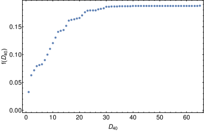
Figure 1: An example of the convergence measure $f$. The $f$ shown is taken from the $p=1.0e-6$ run of the example of section IV and shows the convergence in $D_{40}$, ie the bond linking the spin to the first site of chain $a$, at time $t=10$. The absolute value of $f$ has no meaning, however the fact that it is constant above $D=30$ tells us that increasing $D_{40}$ above this value will have very little effect on the projection error. The fact that the gradient of $f$ is non-monotonic suggests an optimization is possible via the re-ordering of the $Q_{2}$ states.

IV Non-equilibrium steady-states in two-temperature open systems

In this section we demonstrate the utility and power of our method for open quantum systems with numerical simulations of a two-level system strongly and simultaneously coupled to two bosonic baths at different temperatures. This class of two-environment models has both wide-ranging practical applications - such as studying heat and charge transfer in nanodevices benenti_fundamental_2017 ; dubi_colloquium_2011 ; dhar_heat_2008 , as well as fundamental relevance for quantum thermodynamics, decoherence, and non-equilibrium steady states guo_critical_2012 ; zhou_symmetry_2015 ; bruognolo_two-bath_2014 ; segal_spin-boson_2005 ; chen_steady_2020 .

Here we consider two baths, labeled $a$ and $b$, with identical linear couplings and spectral densities, at different inverse temperatures $\beta_{a}$ and $\beta_{b}$ respectively ($\beta=1/T$). The system-bath Hamiltonian is given by

$$\hat{H}=\frac{\omega_{0}}{2}\sigma_{z}+\hat{H}_{I}^{a}+\hat{H}_{I}^{b}+\hat{H}_{B}^{a}+\hat{H}_{B}^{b},$$ (22)

where

$$\hat{H}_{I}^{a}=\sigma_{x}\otimes\sum_{k}(g_{k}^{*}\hat{a}_{k}+g_{k}\hat{a}_{k}^{\dagger})$$ (23)

$$\hat{H}_{I}^{b}=\sigma_{x}\otimes\sum_{k}(g_{k}^{*}\hat{b}_{k}+g_{k}\hat{b}_{k}^{\dagger})$$ (24)

$$\hat{H}_{B}^{a}=\sum_{k}\omega_{k}\hat{a}_{k}^{\dagger}\hat{a}_{k}$$ (25)

$$\hat{H}_{B}^{b}=\sum_{k}\omega_{k}\hat{b}_{k}^{\dagger}\hat{b}_{k}.$$ (26)

The bath parameters are defined in terms of the spectral density $J(\omega)\equiv\pi\sum_{k}|g_{k}|^{2}\delta(\omega-\omega_{k})$ which we take to be Ohmic with a hard cut-off at frequency $\omega_{c}$

$$J(\omega)=2\pi\alpha\omega\theta(\omega_{c}-\omega).$$ (27)

The initial condition $\hat{\rho}(0)$ is taken to be an uncorrelated (product) state of the spin and baths, which - because of the baths’ finite temperatures - must be described by a mixed state, i.e. a density matrix

$$\hat{\rho}(0)=\ket{\uparrow_{z}}\bra{\uparrow_{z}}\otimes\frac{e^{-\hat{H}_{B}^{a}\beta^{a}}}{\operatorname{Tr}\{e^{-\hat{H}_{B}^{a}\beta^{a}}\}}\otimes\frac{e^{-\hat{H}_{B}^{b}\beta^{b}}}{\operatorname{Tr}\{e^{-\hat{H}_{B}^{b}\beta^{b}}\}}.$$ (28)

Remarkably, despite the initial condition containing two statistically mixed thermal density matrices, it has recently been shown by Tamescello et al. that the reduced dynamics of the spin can be obtained from a single MPS simulation of a pure system-environment wave function tamascelli_nonperturbative_2018 ; tamascelli_efficient_2019 . This follows from the formal equivalence of the influence function of a physical environment at inverse temperature $\beta$ with a spectral density $J(\omega)$ and a proxy, zero-temperature environment that is extended over both positive and negative frequencies and which possesses an effective, $\beta$-dependent spectral density $J(\omega,\beta)$ - see Refs. tamascelli_efficient_2019 ; tamascelli_nonperturbative_2018 ; tamascelli_supplemental_nodate . The thermal behavior of the environment is then exactly reproduced using a set of initially empty modes of positive and negative frequencies. This is possible due to the fact that the system cannot distinguish between the occupation of an initially empty negative mode and the depletion of an initially occupied positive mode. A similar idea, formulated in terms of two-mode squeezed states, is at the heart of the thermofield approach of Ref. de_vega_how_2015 , where one can directly see how the relative couplings to modes at $\pm\omega$ enforce the property of detailed balance contained in the physical correlation function of the original, finite-temperature environment.

Following the introduction of the effective $J(\omega,\beta)$, it then becomes possible to apply a unitary transformation of the harmonic environment - the so-called chain mapping chin_exact_2010 ; de_vega_how_2015 - which maps the two baths onto two separate $1D$, nearest-neighbour tight-binding chains that couple at one end to the spin. The resulting transformed system, which is formally equivalent to the initial open system problem, is shown in Fig. 3 The hopping parameters and site energies of the bosonic chains are determined completely by the effective spectral density $J(\omega,\beta)$.

We denote the transformed bath operators as

$$\hat{A}_{n}=\sum_{k}U_{kn}(\beta_{a})\hat{a}_{k}$$ (29)

$$\hat{B}_{n}=\sum_{k}U_{kn}(\beta_{b})\hat{b}_{k},$$ (30)

and our transformed initial condition is

$$\ket{\psi}=\ket{0}_{a}\otimes\ket{\uparrow_{z}}\otimes\ket{0}_{b},$$ (31)

where $\ket{0}_{a(b)}$ is the vacuum state of bath $a(b)$. Physically, such an initial condition could correspond to the sudden connection of two reservoirs by a qubit or few-state nanoscopic junction. Since $\ket{\psi}$ is a product state, it can be represented as an MPS with all bond-dimensions equal to 1. Under conventional 1TDVP it would not be possible to use such an initial MPS since the bond-dimensions would be fixed at 1 throughout the whole simulation, thus only capturing the on-site evolution. However, with our bond-adaptive 1TDVP method we are able to start from this extremely simple initial condition and the increase the bond-dimensions on the fly to capture the growing entanglement, as, when and where it is needed.

IV.1 Numerical results and observations of transient heat flows

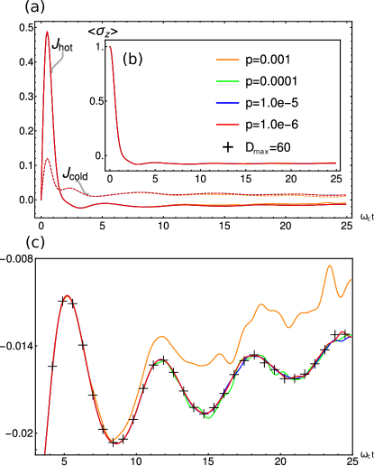
Figure 2: Dynamics of a two level system with splitting $\omega_{0}=0.2\omega_{c}$ coupled between two harmonic baths, temperatures $\beta_{a}=100/\omega_{c}$, $\beta_{b}=1/\omega_{c}$, with Ohmic spectral densities, coupling strength $\alpha=0.2$. The Foch spaces of the bath modes were truncated to $15$ states. Results were obtained using 1TDVP with dynamic bond-dimensions for 4 different values of the precision $p$ and $D_{lim}=60$ and checked against conventional 1TDVP with $D_{max}=60$. (a) $\langle\hat{J}_{a}(t)\rangle$ (dashed line) and $\langle\hat{J}_{b}(t)\rangle$ (solid line). (b) $\langle\sigma_{z}(t)\rangle$ ($\langle\sigma_{x}(t)\rangle=\langle\sigma_{y}(t)\rangle=0$). (c) Expanded view of $\langle\hat{J}_{b}(t)\rangle$, black crosses show results obtained from fixed bond-dimension 1TDVP.

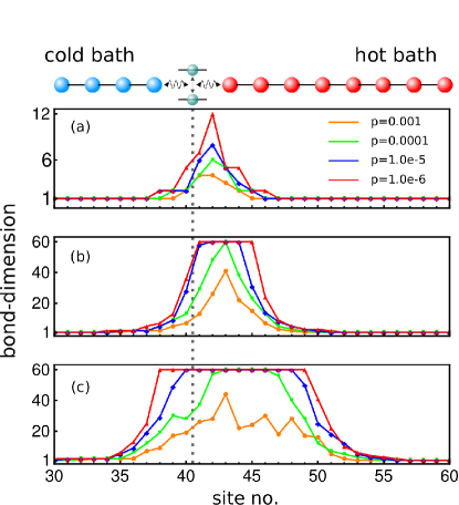
Figure 3: Bond-dimensions at times $\omega_{c}t=1$ (a), $\omega_{c}t=5$ (b) and $\omega_{c}t=10$ (c). The spin is on site 41 of the chain. The bond-dimensions grow faster and expand away from the spin quicker for the hot bath than for the cold bath, reflecting the different computational resources necessary to simulate them.

We run the dynamics with four values of the precision $p$ to show convergence. For simplicity and speed we set the local limit $D_{lim}=60$. For comparison we also ran the simulation with conventional 1TDVP with a fixed maximum bond-dimension $D_{max}=60$. Setting $D_{lim}=60$ guarantees that the dynamic bond-dimension simulations will all be faster than normal 1TDVP at $D_{max}=60$. The Foch spaces of the bath modes are truncated to $15$ states woods_simulating_2015 . The simulations were run on an Intel^® Xeon^® W-2123 Processor. We find that a significant speed up is achieved with the most precise dynamic-bond simulation ($p=1.0e-6$) completing in 1 hour 26 minutes versus 5 hours 55 minutes for the fixed-bond run.

The spin dynamics are shown in fig. 2 for the following choice of parameters in units of $\omega_{c}$: $\beta_{a}=100/\omega_{c},\beta_{b}=1/\omega_{c},\alpha=0.2$ and $\omega_{0}=0.2\omega_{c}$. The chosen value of $\alpha$ is considered non-perturbative for Ohmic baths weiss2012quantum . The spin evolves from its initial pure state of up along $\ket{\uparrow_{z}}$ into a statistical mixture of up and down with a slight predominance for spin down in the steady state, due to the presence of the cold environment (the hot environment has a temperature x20 greater than the spin energy level splitting) (fig. 2(b)).

Another interesting dynamical observable is the heat flow between the spin and the two baths. We define the following operators

$$\hat{J}_{a}=\sigma_{y}\otimes(\hat{A}_{0}^{\dagger}+\hat{A}_{0}),$$ (32)

and

$$\hat{J}_{b}=\sigma_{y}\otimes(\hat{B}_{0}^{\dagger}+\hat{B}_{0}),$$ (33)

which measure the heat flux from the spin to baths $a$ and $b$ respectively. At early times we see from fig. 2(a) that heat flows out of the spin into both hot and cold baths, since the spin begins in an inverted state, and that later a steady state is established in which net heat flows into the spin from the hot bath ($b$) and out of the spin into the cold bath ($a$). We see also from the expanded view of $\hat{J}_{b}$ in fig. 2(c) that these results are well converged w.r.t. the results of the fixed bond-dimension simulation, clearly demonstrating the advantage of our approach.

The bond-dimensions for all four values of $p$ at three different time steps are also shown in fig. 3. We observe that the simulation of the chains becomes more expensive for higher temperatures, and we have traced back to the properties of the chain parameters and effective thermal spectral densities: stronger intra-chain coupling for higher temperature environments causes entanglement between the sites to grow faster and causes excitations to travel faster along the chain. Longer chains are thus required in order to avoid boundary effects, and larger bond dimensions are needed for the stronger quantum correlations across the chain sites. We see from fig. 3 that the new method is able to account for both of these effects when optimizing the bond-dimensions by giving larger bond-dimensions to chain $b$ which propagate outwards faster to match the progress of the perturbation along the chain.

Indeed, we find that this new approach is particularly effective for this class of open system problems, in which the environment is modeled with a chain initialized in the vacuum state. In particular, little thought now has to be paid to the choice of chain lengths since any chain sites not touched by the perturbation will remain with trivial bond-dimensions and so the updates on these sites will take almost no time. Under fixed bond-dimension 1TDVP, however the chain lengths have a significant impact on simulation time and so must be chosen carefully tamascelli_supplemental_nodate . As a very large number of open quantum system problems involve ’impurity’ like dynamics of a spatially localised system with an initiialy uncorrelated environment state, taking full advantage of the evolving range of correlations in an automated way could lead to very efficient ‘black-box’ algorithms for open system problems. This idea may be straight forwardly extended to tree-MPS which will allow the simulation of systems with complex multi-environment interactions, whereupon, the advantages demonstrated here will become even more important and could be further combined with the ‘entanglement renormalisation techniques‘ introduced in Ref. schroder_tensor_2019 for molecular open quantum dynamics.

Finally, analysis of the distribution and development of correlations, as in Fig. 3, can also provide interesting physical insights into the underlying microscopic dynamics, particularly when considering non-equilibrium problems where quantum systems interact with multiple quantum environments, i.e. in nanoscale energy harvesting, transport and sensing. We believe our adaptive 1TDVP could prove very useful in such problems, and perhaps several others types that lie outside of the typical scope of open quantum systems.

References

- (1) U. WeissQuantum dissipative systems Vol. 13 (World scientific, 2012).
- (2) H.-P. Breuer et al., The theory of open quantum systems (Oxford University Press on Demand, 2002).
- (3) A. Chin et al., Nature Physics 9, 113 (2013).
- (4) J.-L. Brédas, E. H. Sargent, and G. D. Scholes, Nature materials 16, 35 (2017).
- (5) G. D. Scholes et al., Nature 543, 647 (2017).
- (6) Y. Ashida, Quantum Many-Body Physics in Open Systems: Measurement and Strong Correlations (Springer Nature, 2020).
- (7) A. Strathearn, P. Kirton, D. Kilda, J. Keeling, and B. W. Lovett, Nature Communications 9, 3322 (2018).
- (8) A. Ishizaki and G. R. Fleming, The Journal of chemical physics 130, 234111 (2009).
- (9) M. Topaler and N. Makri, The Journal of chemical physics 101, 7500 (1994).
- (10) J. Prior, A. W. Chin, S. F. Huelga, and M. B. Plenio, Physical review letters 105, 050404 (2010).
- (11) S. Oviedo-Casado et al., Phys. Rev. A 93, 020102 (2016).
- (12) A. D. Somoza, O. Marty, J. Lim, S. F. Huelga, and M. B. Plenio, Phys. Rev. Lett. 123, 100502 (2019).
- (13) C. J. Lindner, F. B. Kugler, V. Meden, and H. Schoeller, Physical Review B 99, 205142 (2019).
- (14) H. Wang and J. Shao, The Journal of Physical Chemistry A 123, 1882 (2019).
- (15) J. Haegeman, C. Lubich, I. Oseledets, B. Vandereycken, and F. Verstraete, Physical Review B 94, 165116 (2016), arXiv: 1408.5056.
- (16) J. Haegeman et al., Physical Review Letters 107, 070601 (2011).
- (17) F. A. Y. N. Schröder and A. W. Chin, Phys. Rev. B 93, 075105 (2016).
- (18) C. Gonzalez-Ballestero, F. A. Y. N. Schröder, and A. W. Chin, Phys. Rev. B 96, 115427 (2017).
- (19) R. Orus, Annals of Physics 349, 117 (2014), arXiv: 1306.2164.
- (20) U. Schollwöck, Annals of Physics 326, 96 (2011).
- (21) S. Paeckel et al., Annals of Physics 411, 167998 (2019), arXiv: 1901.05824.
- (22) D. Bauernfeind and M. Aichhorn, SciPost Physics 8, 024 (2020), arXiv: 1908.03090.
- (23) C. Hubig, I. P. McCulloch, and U. Schollwöck, Physical Review B 95, 035129 (2017), arXiv: 1611.02498.
- (24) Z. Li, M. J. O’Rourke, and G. K.-L. Chan, Physical Review B 100, 155121 (2019), arXiv: 1907.06018.
- (25) V. Murg, J. I. Cirac, B. Pirvu, and F. Verstraete, New Journal of Physics 12, 025012 (2010), arXiv: 0804.3976.
- (26) P. Secular et al., arXiv:1912.06127 [cond-mat, physics:physics, physics:quant-ph] (2020), arXiv: 1912.06127.
- (27) E. Leviatan, F. Pollmann, J. H. Bardarson, D. A. Huse, and E. Altman, arXiv:1702.08894 [cond-mat, physics:quant-ph] (2017), arXiv: 1702.08894.
- (28) S. Goto and I. Danshita, Physical Review B 99, 054307 (2019), arXiv: 1809.01400.
- (29) G. Vidal, Physical Review Letters 93, 040502 (2004), Publisher: American Physical Society.
- (30) A. J. Daley, C. Kollath, U. Schollwoeck, and G. Vidal, Journal of Statistical Mechanics: Theory and Experiment 2004, P04005 (2004), arXiv: cond-mat/0403313.
- (31) S. R. White and A. E. Feiguin, Physical Review Letters 93, 076401 (2004), Publisher: American Physical Society.
- (32) E. J. Heller, The Journal of Chemical Physics 64, 63 (1976).
- (33) C. Hubig, J. Haegeman, and U. Schollwöck, Physical Review B 97, 045125 (2018).
- (34) C. Lubich, I. Oseledets, and B. Vandereycken, SIAM Journal on Numerical Analysis 53, 917 (2015), arXiv: 1407.2042.
- (35) F. A. Y. N. Schröder, D. H. P. Turban, A. J. Musser, N. D. M. Hine, and A. W. Chin, Nature Communications 10, 1062 (2019).
- (36) X. Xie et al., The Journal of Chemical Physics 151, 224101 (2019).
- (37) C. Hubig, I. P. McCulloch, U. Schollwöck, and F. A. Wolf, Physical Review B 91, 155115 (2015).
- (38) D. Tamascelli, A. Smirne, J. Lim, S. F. Huelga, and M. B. Plenio, Physical Review Letters 123, 090402 (2019), arXiv: 1811.12418.
- (39) S. Descombes and M. Thalhammer, IMA Journal of Numerical Analysis 33, 722 (2013), Publisher: Oxford Academic.
- (40) C. Lubich, From Quantum to Classical Molecular Dynamics: Reduced Models and Numerical Analysis (European Mathematical Society, 2008), Google-Books-ID: 11brUAQLvZoC.
- (41) H. F. Trotter, Proceedings of the American Mathematical Society 10, 545 (1959).
- (42) B. Vanhecke, M. Van Damme, J. Haegeman, L. Vanderstraeten, and F. Verstraete, arXiv:2001.11882 [cond-mat, physics:quant-ph] (2020), arXiv: 2001.11882.
- (43) M. Hochbruck and C. Lubich, SIAM Journal on Numerical Analysis 34, 1911 (1997), Publisher: Society for Industrial and Applied Mathematics.
- (44) G. Benenti, G. Casati, K. Saito, and R. Whitney, Physics Reports 694, 1 (2017).
- (45) Y. Dubi and M. Di Ventra, Reviews of Modern Physics 83, 131 (2011).
- (46) A. Dhar, Advances in Physics 57, 457 (2008).
- (47) C. Guo, A. Weichselbaum, J. von Delft, and M. Vojta, Physical Review Letters 108, 160401 (2012).
- (48) N. Zhou, L. Chen, D. Xu, V. Chernyak, and Y. Zhao, Physical Review B 91, 195129 (2015).
- (49) B. Bruognolo et al., Physical Review B 90, 245130 (2014).
- (50) D. Segal and A. Nitzan, Physical Review Letters 94, 034301 (2005).
- (51) T. Chen, V. Balachandran, C. Guo, and D. Poletti, arXiv:2004.05017 [cond-mat] (2020), arXiv: 2004.05017.
- (52) D. Tamascelli, A. Smirne, S. Huelga, and M. Plenio, Physical Review Letters 120, 030402 (2018).
- (53) D. Tamascelli, A. Smirne, S. F. Huelga, and M. B. Plenio, p. 4.
- (54) I. de Vega, U. Schollwöck, and F. A. Wolf, Physical Review B 92, 155126 (2015), arXiv: 1507.07468.
- (55) A. W. Chin, A. Rivas, S. F. Huelga, and M. B. Plenio, Journal of Mathematical Physics 51, 092109 (2010), arXiv: 1006.4507.
- (56) M. Woods, M. Cramer, and M. Plenio, Physical Review Letters 115, 130401 (2015).