Convergence and optimality of an adaptive modified weak Galerkin finite element method
Abstract.
An adaptive modified weak Galerkin method (AmWG) for an elliptic problem is studied in this paper, in addition to its convergence and optimality. The modified weak Galerkin bilinear form is simplified without the need of the skeletal variable, and the approximation space is chosen as the discontinuous polynomial space as in the discontinuous Galerkin method. Upon a reliable residual-based a posteriori error estimator, an adaptive algorithm is proposed together with its convergence and quasi-optimality proved for the lowest order case. The primary tool is to bridge the connection between the modified weak Galerkin method and the Crouzeix-Raviart nonconforming finite element. Unlike the traditional convergence analysis for methods with a discontinuous polynomial approximation space, the convergence of AmWG is penalty parameter free. Numerical results are presented to support the theoretical results.
Key words and phrases:
modified weak Galerkin, adaptive methods, a posteriori error estimation, convergence, optimality1991 Mathematics Subject Classification:
65N15, 65N30, 65N501. Introduction
Consider the following model second-order elliptic problem
| (1.1) | ||||
where is a bounded polygonal or polyhedral domain in . Assume that an initial conforming partition of exists and for all , the coefficient is assumed to be a piecewise constant with respect to this partition.
Weak Galerkin (WG) is a novel numerical method for solving partial differential equations in which classical differential operators (such as gradient, divergence, curl) are approximated in a weak sense. WG method was initially introduced in [53, 54, 41] for the second-order elliptic problem. Since then, the WG method has successfully found its way to many applications, for example, elliptic interface problems [37], Helmholtz equations [43, 40, 22], biharmonic equations [38, 42], Navier-Stokes equations [34, 27], electromagnetic problems [44, 49, 7], and its solvers [13, 30], etc. In particular, Wang et al. [55] introduced a modified weak Galerkin (mWG) method for the Poisson equation. The mWG method has been successfully applied to, such as parabolic problem [23], Signorini and obstacle problem [58], and Stokes equations [51]. More recently, Cui et al. generalized the mWG to biharmonic problems [19]; Li et al. showed the mWG is robust for singularly perturbed reaction-diffusion problems [32]; Wang et al. presented an mWG method in a mixed form in [56]. For other contributions in mWG variants, we also refer the readers to [31, 4, 25, 29].
The solution to (1.1) may contain singularities. To approximate problem (1.1) efficiently, the general practice is to adopt adaptivity by designing an adaptive finite element cycle through the help of the a posteriori error estimators, a bulk marking strategy, and certain local refinement techniques. As examples non-convergent adaptive algorithms [14] may fail to produce the desired approximation even with additional iterations, the convergence analysis of an adaptive algorithm is of fundamental importance for ensuring that the correct approximation is obtained. It theoretically guarantees that the correct approximation will be obtained, especially if one wants to avoid the situation when more computational resources may go wasted after iterative refinements.
The convergence theory of adaptive finite element methods is relatively mature, see [45] and the references therein. Nevertheless, few research results exist for the a posterior error estimates for WG methods. Chen et al. [12] presented the a posteriori error estimates for second-order elliptic problems; Zhang and Chen [59] proposed a residual-type error estimator and proved global upper and lower bounds of the WG method for second-order elliptic problems in a discrete -norm; Li et al. [33] introduced a simple a posteriori error estimator which can be applied to general meshes such as hybrid, polytopal and those with hanging nodes for second-order elliptic problems; Mu [35] presented an a posteriori error estimate for the second-order elliptic interface problems; Zheng and Xie [61] discussed a residual-based a posteriori error estimator for the Stokes problem. There are only a few research results for a posteriori error estimates for mWG methods. Zhang and Lin [60] proposed an a posteriori error estimator for the second-order elliptic problems. Tang et al. proposed an adaptive mWG for -elliptic problems in [50].
This paper aims to prove the optimal convergence of an AmWG algorithm for the second-order elliptic problem (1.1). Different from the mWG originally introduced in [55], we simplify the mWG as follows: for a weak function , the edge/face term is not independent anymore as we choose , i.e., is obtained through averaging the interior discontinuous variable and then projected through to a one-degree-lower polynomial space. Compared with interior-penalty discontinuous Galerkin(IPDG) (see e.g.[2]), the mWG is stable without choosing a sufficiently large penalty parameter. This simplification ( opposed to in [55]) brings extra difficulty to the analysis of convergence. The reason is that a simple port of the workflow presented in [5], by decomposing the discontinuous approximation space into a continuous subspace and its orthogonal complement, will introduce a penalty parameter that is not originally in the mWG discretization (c.f. [57]). To our best knowledge, there is no literature on the convergence of adaptive mWG methods with the skeletal variable being one degree lower than the internal variable.
To conquer this difficulty, by introducing an interpolation operator onto the Crouzeix-Raviart type nonconforming finite element space , we bound the stabilization term and prove an a posteriori error estimate in the discrete -norm. One main ingredient in the convergence analysis of a standard adaptive procedure is the orthogonality of the error to the finite element space. However, such an orthogonality does not hold for mWG approximations. Instead, a quasi-orthogonality result is established. Hu and Xu [26] defined a canonical interpolation operator for the lowest Crouzeix-Raviart type nonconforming finite element space and established the quasi-orthogonality property for both the velocity and the pressure in the Stokes problem. The main observation is that the modified weak gradient for a function is equal to the elementwise gradient of the interpolant , namely and we can derive the desired quasi-orthogonality property for the lowest order (-) mWG.
Another key component to establish the optimality of the adaptive algorithm is the localized discrete upper bound for the a posteriori error estimator. By using a prolongation operator introduced in [26], we are able to derive the discrete reliability and use it to prove the optimality of the convergence.
For the a posteriori error analysis of mWG approximations, we mainly follow Bonito and Nochetto [5] and Chen, Wang and Ye [12]. For the analysis of the convergence and the optimality of adaptive procedure, we mainly use the Hu and Xu [26] and Huang and Xu [28]. We do not claim any originality on the proof of convergence and optimality. Instead, the main contribution of this paper is to bound the stabilization term by the element-wise residual and flux jump, as well as to establish a quasi-orthogonality and a discrete upper bound which are important ingredients on the convergence theory of adaptive finite element methods.
The rest of this paper is organized as follows. In Section 2, the definitions of weak gradient and discrete weak gradient are introduced, as well as the modified weak Galerkin finite element spaces and the corresponding bilinear form . In Section 3, a residual-type error estimator is constructed, and its reliability and efficiency are shown. In Section 4, we introduce an adaptive modified weak Galerkin method (AmWG) and prove its convergence and optimality. Some numerical examples are presented in Section 5 to verify the theoretical results.
2. Notation and Preliminary
The goal of this section is to present the modified weak Galerkin (mWG) formulation for (1.1). First, the standard weak Galerkin method is reviewed, then an mWG finite element space and the discretization thereof are introduced.
2.1. Weak Galerkin Methods
Given a polygonal/polyhedral element with boundary , the notation defines a weak function on such that and . Subsequently, the weak function space on is defined as
Let be the set of polynomials on with degree no more than (). The discrete weak gradient operator is defined for polynomial functions. With slight abuse of notation, when no ambiguity arises, we shall denote as , which should be clear from the context.
Definition 2.1 ([39, Definition 2.1]).
The discrete weak gradient operator, denoted by , is defined as the unique polynomial satisfying the following equation for
| (2.1) |
In the definition above, is the outward normal direction to , is the -inner product of and , and is the -inner produce of and . The differential operators involved are well-defined when restricted to one element. In the context of the gradient operator defined across multiple elements in , the elementwise gradient is introduced, i.e., in element .
In the rest of the paper, we restrict ourselves to a shape-regular triangulation of . denotes the set of all the edges or faces in , and is the set of all the interior edges or faces. Denote the -dimensional Lebesgue measure. For , its associated patch as . For a set , its associated patch element patch is .
Given a positive integer , the -th order weak Galerkin finite element space on is defined as follows:
| (2.2) |
and the one with zero boundary condition:
| (2.3) |
Note that is single-valued on each .
For , the discrete bilinear form for the variational form of problem (1.1) is defined as
| (2.4) |
where the weak gradient , and is the projection from to on an . Again when it is clear from the context, we shall omit the degree of the polynomial involved in the projection operator.
The weak Galerkin discretization is: to find a satisfying
| (2.5) |
The WG discretization (2.5) is well-posed as defines an inner product on the space .
For completion and the convenience of our readers, we include a short argument here to show that
| (2.6) |
defines a norm in . Assume that , then on every element and on every , then by definition (2.1)
which implies on . As a result, is constant on . Moreover, on each . Knowing on . By an argument of continuation, . Therefore, defines a norm and defines an inner product on the space .
The proof above reveals that the boundary part can be set as a polynomial with degree one less than that of the interior one since its presence is only in .
2.2. Modified weak Galerkin finite element
Let be the common edge/face shared by two elements , and denote by . We assume that globally each is associated with a fixed unit normal vector . When , we can get ’s tangential vector by , which is obtained by rotating clockwise by . Without loss of generality, the is assumed pointing from to . Denote by and the outer unit normal vectors with respect to and , respectively. For a smooth enough scalar function , we define its average and jump on by
Similarly, for an admissible vector function , we have
In the definitions above, and ’s values on are defined for those spaces which yield a well-defined trace, respectively.
Specifically, in discretization (2.5), is chosen to be in the discontinuous polynomial space
and the edge/face term . Now a weak function is , which offers a continuous embedding of with respect to norm (2.6), which will be shown equivalent to the modified IP norm associated with (2.10). The modified weak Galerkin finite element space for is then defined as
| (2.7) |
and
| (2.8) |
Remark 2.2.
The definition of the weak gradient is modified accordingly as follows.
Definition 2.3.
The modified weak gradient operator acting on any , denoted by on , is defined as the unique polynomial in such that its inner product with any satisfies the following equation:
| (2.9) |
When the triangulation is clear from the context, we shall abbreviate the notation as .
Let be the common edge/face shared by . By using the mWG space (2.7) in the WG bilinear form (2.4), one can simplify the stabilization term on for and , henceforth the same argument applies to other edges/faces.
Consequently, for , the associated bilinear form is defined as
| (2.10) | |||||
A modified weak Galerkin (mWG) approximation is then to seek satisfying
| (2.11) |
It is clear that the modified weak Galerkin finite element scheme (2.11) is also well-posed since the problem is solved in a subspace (the embedding of the DG space) of the original WG space. If nonhomogeneous Dirichlet boundary condition on is presented, can be decomposed to the sum of two parts, the first part satisfies the approximation problem above. For the second part, the boundary contribution is which can be moved to the right-hand side in addition to the source term. For other treatments of the boundary data such as interpolations, see e.g., [36].
Remark 2.4.
In the classic IPDG formulation (see e.g., [5]), for , the bilinear form is
| (2.12) | |||||
In comparison, in (2.10), using the definition of the weak gradient, several times of the integration by parts, and the assumption that is a piecewise constant, for , an equivalent bilinear form of (2.10) reads
| (2.13) | |||||
The only difference is that one in (2.12) is replaced by in (2.13). This minor change leads to a major improvement that the mWG (2.11) is automatically coercive and continuous as the bilinear form induces a norm. While in IPDG (2.12), the penalty parameter being sufficiently large is a necessary condition to achieve the coercivity both theoretically and numerically [48].
The following quantity is well-defined for and defines a mesh dependent norm on (for similar results see e.g., [39])
| (2.14) |
We note that (2.14) defines a norm on naturally, since is a subspace of the bigger space and is equivalent to (2.6) restricted to this subspace; see (2.6) and the proof afterwards.
With slight abuse of notation, we are interested in estimating the following error using computable quantities and designing a convergent adaptive algorithm to reduce its magnitude successively:
| (2.15) |
3. A Posteriori Error Analysis
In this section, we shall prove the reliability and efficiency of a residual-type error estimator. For , we define the element-wise error estimator as
| (3.1) | |||||
where and for . The element residual is defined as
and the normal jump of the weak flux is defined as
For the tangential jumps, when :
and when
Then the error estimator for the set is defined as
| (3.3) |
In computing the error estimator, only the information of is used. Thus, we opt for a notation of instead of . In Remark 4.1, some further explanation is given with regard to this choice of the notation for the error estimator in the context of the convergence analysis.
3.1. A space decomposition
In this section, a space decomposition is first introduced to bridge the past result of the full degree jump to with one less degree. Then, similar to [5], a partial orthogonality for the mWG approximation is introduced to enable the insertion of continuous interpolants to prove the reliability.
For consisting of discontinuous polynomial of degree :
| (3.4) |
where is the continuous Lagrange finite element space. is a subspace of so that their quotient space is endowed with the induced topology of the seminorm . When , is simply the well-known Crouzeix-Raviart finite element space [18]. When , is a generalization of the Crouzeix-Raviart type nonconforming finite element space [15], which can be viewed a special case of nonconforming virtual element [3] restricted on triangulations:
| (3.5) |
where
| (3.6) |
Unlike the virtual element space, where the shape function may not be polynomials, it is shown in [17, 15] that the space can be obtained from by adding locally supported polynomial bases. More specifically, in [15], the authors constructed a set of nodal basis for a strict subspace of while satisfying the continuity constraint (3.6). However, to serve the purpose of this paper, is to bridge the proofs, it only suffices to know the existence of a set of unisolvent degrees of freedom, while not explicitly construct the dual basis of it. We refer the reader to [3, Section 3.2] for the degrees of freedom for general polytopes which includes the case of triangulations () in this paper.
When restricted a smaller subspace , the weak gradient coincides with the piecewise gradient, and the stabilization is vanished which leads to the following partial orthogonality.
Proof.
It follows from that . In addition, for functions when , thus in , which further implies . Lastly since implies that for any , as a result, and the lemma follows. ∎
The following interpolation operator to the nonconforming space will play an important role in the analysis.
Lemma 3.2.
There exist an interpolation operator , which is locally defined and a projection, as well as a constant depending only on the shape regularity of such that for all the following inequality hold: for ,
| (3.8) |
Proof.
The proof follows a similar argument as the one in [5, Lemma 6.6], and is presented here for completion. Denote the set of the degrees of freedom functionals in as , and the nodal bases set is corresponding to . Let , where is either a single element or , then we consider the following projection obtained through
| (3.9) |
and then the interpolation is defined as:
| (3.10) |
If , we have locally on , thus , and is a projection.
Moreover, implies that , as well as by (3.9), hence by a scaling argument and the equivalence of norms on a finite-dimensional space, we have
| (3.11) |
where we note that if a nodal basis has support , both sides of the inequality above will be 0, as the projection (3.9) modulo out the element bubbles.
Next, consider on a , and all local degrees of freedom of which the nodal basis having support overlaps with , we have on
| (3.12) |
On , is either defined on (see [3, Section 3.2])
or defined on ()
and in both cases, we have by a simple scaling argument and by (3.11)
Lastly, combining the estimate above with (3.12), using the fact that , and estimate (3.11) yields the desired estimate. ∎
3.2. Reliability
In this section, the global reliability of the estimator in (3.3) is to be shown. The difference between the weak gradient and classical gradient can be controlled by the jump term which becomes a handy tool in our analysis.
Lemma 3.3.
For , it holds for any
Proof.
The proof follows from [60, Lemma 2.1] with coefficient added and a more localized version is presented. On , let , applying integration by parts on and the weak gradient definition (2.9) on , we have
where the plus or minus sign depends on whether the outward normal for coincides with the globally defined normal for this edge/face. Now by a standard trace inequality and an inverse inequality, we have
then the desired result follows by canceling a and summing up the element-wise estimate for every . ∎
Next we bound the stabilization term by the element-wise residual and the normal jump of the weak flux. We note that in [61], though focusing on a different model problem, the -weighted solution jump can be used as the sole error estimator to guarantee reliability and efficiency up to data oscillation. Nevertheless, the motivation here is to change the dependence of the error indicators on the local mesh size from to , so that a contraction property of the estimator can be proved in Section 4.2 without any saturation assumptions, which is one of the keys to show the convergence of an adaptive algorithm.
Lemma 3.4.
Proof.
The proof of the upper bound mainly follows the paradigm in [12, 11, 1]. Without loss of generality, the presentation is for . We shall use the Helmholtz decomposition of .
Theorem 3.5 (Upper Bound).
Proof.
We first give an outline of our proof. The following Helmholtz decomposition ([20, 8], see also [12, Lemma 4.2], Chapter I Theorem 3.4 and Remark 3.10 in [24]) commonly used for nonconforming elements is applied to :
| (3.15) |
where , and . The decomposition satisfies
| (3.16) |
Moreover, can be chosen to be divergence-free so that it is piecewise -smooth (e.g., see [6, Appendix A]) such that
| (3.17) |
- (1)
- (2)
A key result (Lemma 3.4) is applied here to bound the stabilization term by the element-wise residual and the normal jump of the flux, where the quasi-interpolant to is used. As a result, we turn our focus onto the error without the stabilization as follows
| (3.18) |
Let be the robust Clément-type quasi-interpolation (e.g., see [47]) for such that the following estimates holds,
| (3.19) |
Using the partial orthogonality (3.7), integrating by parts for , Cauchy-Schwarz inequality, and estimates in (3.19), we have
where the constant depends on the shape-regularity of .
For in (3.18), we need a robust Clément-type interpolation (see [6, Theorem 4.6]) satisfying:
| (3.20) |
It is straightforward to verify that, by the definition of the modified weak gradient (2.9) and the fact that , we have
Consequently, as and can be inserted to obtain the following:
| (3.21) |
Upon an integration by parts, will appear in each element, in general, this is not zero as is computed in the sense of distribution. To handle this term, simply notice that element-wise, by Lemmas 3.3 and 3.4, and an inverse inequality
| (3.22) | |||||
Integrating by parts on (3.21), applying (3.22), we have
3.3. Efficiency
The standard bubble function technique is opted (see [52]) to derive the efficiency bound, while the tangential jump part’s proof follows a standard argument of the a posteriori error estimation for standard WG discretization in [12]. As the proofs are standard, we only present the results here.
For and , the oscillation is defined to be
| (3.24) |
where denotes the projection onto the set of either the piecewise on , where if and when .
For any subset , we define
| (3.25) |
Note that, on , using the properties of the -projection, the oscillation are dominated by the estimator; namely,
| (3.26) |
Theorem 3.7.
(Local lower bound) For all , there holds
| (3.27) |
where the constant only depends on the shape regular of .
4. An Adaptive Modified Weak Galerkin Method
In this section, first we introduce an adaptive modified weak Galerkin method (AmWG). Next, a quasi-orthogonality is proved and is further exploited to derive the convergence of AmWG. At last, we shall present the discrete reliability and propose the quasi-optimality of the AmWG.
Henceforth, the polynomial degree is chosen to be , the reason for this is that we shall borrow some classical results for Crouzeix-Raviart element to establish a penalty parameter-free convergence. Notice that the penalty parameters in schemes based on discontinuous approximation spaces are indispensable not only for the coercivity (Remark 2.4), but also for the convergence of adaptive algorithms due to the lack of a direct orthogonality result (see e.g., [5]). For a similar nonconforming method [46], one still needs to choose a sufficiently large penalty parameter to prove the convergence. By bridging the connections between the lowest order WG method and Crouzeix-Raviart element, we are able to show the convergence without the presence of a sufficiently large penalty.
4.1. Algorithm
| (4.1) |
In the SOLVE step, given a function and a triangulation , the exact discrete solution is sought . In this step, we assume that the discrete linear system associated with problem (2.11) can be solved exactly.
In the ESTIMATE step, local error indicators and the global estimator are calculated.
In the MARK step, a set of marked elements is obtained by the Dörfler marking strategy [21] applied on the error indicators on obtained in the ESTIMATE step.
In the REFINE step, different from traditional DG approaches which allow hanging nodes (e.g., [5]), the marked elements, as well as their neighbors, are refined using bisection () or red-green refinement () while preserving the conformity of the triangulation.
In the paragraphs hereafter, the notation stands for that is a refinement of following the marking strategy above, where , and here denotes the set of triangulations which are conforming (no hanging nodes), shape regular and refined from an initial triangulation .
While showing the lemmas related to the convergence of the AmWG, for and , the set of refined elements in , which become new elements in , is denoted as
Whenever the dependence of the weak gradient on two different meshes becomes relevant, the weak gradient’s notation is changed accordingly to emphasize the mesh of the function defined on, for example, the piecewisely defined weak gradient is for any . When its restriction to one element is of interest, is used.
Remark 4.1.
The reason why we opt for a notation , not is as follows. As in the context of the convergence analysis, this chosen notation has a more consistent meaning when considering two meshes: one is refined from the other. Note that for two nested triangulation , the weak gradient of a coarse function on the fine mesh is different with the weak gradient on the coarse grid . To be specific, on with , is different from . We note that this is different from that of the piecewise gradient .
4.2. Reduction of error estimator
The next lemma shows the reduction of the error estimator after the mesh is refined. On a refined mesh, the effect of changing the finite element function for is as follows.
Lemma 4.2.
For with , for any , , and , there exists a constant depending on the shape regularity such that
| (4.3) | ||||
We can also get the contraction of if the weak flux of the solution remains invariant and is interpolated into a finer mesh refined using the Dörfler marking strategy.
Here we skip the proof of Lemmas 4.2 and 4.3, since the corresponding techniques are quite standard and can be found, e.g. in [9].
Hereafter the following short notations are adopted: on , denotes the weak gradient, and denotes the piecewise gradient , for quantities involving two levels of meshes, the subscript follows that of the coarse one.
Lemma 4.4.
For the two consecutive triangulation in the AmWG cycle (1), and any , there exists a constant depending on the shape regularity such that
| (4.5) |
Proof.
For the contraction of , there is no extra factor as an artifact of Young’s inequality, and this will play a key role in proving the convergence without any penalty parameter on the stabilization.
Lemma 4.5.
Let be the refinement of produced in Algorithm 1. There exists a constant satisfying
| (4.6) |
Proof.
For any , we only need to consider the case where is subdivided into with , we have
where . ∎
Lemma 4.6.
4.3. Quasi-orthogonality
In this section, we will show the contraction property of the energy error by using similar arguments in [26].
First, a canonical interpolation operator is defined any : satisfies
| (4.9) |
and the interpolation admits the following estimate:
| (4.10) |
where the constant depends only on the shape regularity of .
Lemma 4.7.
Assume that is a constant vector on each element , we have
| (4.11) |
Proof.
Note that is a constant vector on each , . By applying integration by parts, we will get the desired result. ∎
For , it is embedded into by . Denote the interpolant for satisfying
| (4.12) |
Lemma 4.8.
For any and , the interpolation defined in (4.12) satisfies
| (4.13) |
Proof.
For any constant vector , using the definition (2.3) leads to
As are constant on each element , we get (4.13). ∎
Lemma 4.9 (Quasi-orthogonality).
4.4. Convergence of AmWG
In the following theorem, the convergence of Algorithm 1 is proved. The main idea is to use the negative term on the right to cancel the positive terms, and to use the reduction factor in (4.6) and (4.7).
Theorem 4.10.
Given a marking parameter and an initial mesh . Let be the solution of (1.1), be a sequence of meshes, finite element approximations and error estimators produced by Algorithm 1 with , then there exist constants , , depending only on the shape regularity of , the marking parameter , and , such that if
then
where the constant is given by Theorem 3.5.
Proof.
By recursion, the decay of the error plus the estimator is as follows.
4.5. Discrete Reliability
In this section, we prove the discrete reliability. Let be a refinement from , we recall the projection operator (see [26, Section 5]).
Lemma 4.12 ([26], Lemma 5.1).
For any , it holds that
| (4.19) |
Remark 4.13.
Lemma 4.12 was presented in [26] for Stokes problem with a vector function in the Crouzeix-Raviart space, with a bound using on an edge (2D). However, since the proof only relies on the scaling of the nodal basis function, and a partition of unity property of the basis on an edge, both of which holds in 3D tetrahedral nodal basis associated with faces, the result holds for scalar functions by choosing only 1 non-trivial component in the vectorial result, and acknowledging the fact that if is a face on .
Lemma 4.14.
The following discrete reliability holds with constant depending on the shape regularity of the mesh
| (4.20) |
Proof.
By Lemma 4.7 and 4.8, we obtain
| (4.21) | |||||
For the first term on the right-hand side of the equation above, denote , it follows from , that
and for a constant vector on
Combining both further implies
| (4.22) | |||||
For the second term in (4.21), together with Lemma 4.8, applying the Cauchy-Schwarz inequality implies
| (4.23) | |||||
4.6. The Optimality of the AmWG
In this section, the optimality of the AmWG Algorithm 1 will be shown. First a Céa-type lemma can be obtained as follows.
Lemma 4.15.
There exists a constant depending only on the shape regularity of such that
| (4.25) | |||||
Proof.
The application of Strang’s lemma [16] yields
| (4.26) | |||||
We need to define the following higher order conforming finite element space
| (4.27) |
there exists an interpolation with following properties (see [26, Section 6])
| (4.28) | ||||
for , edge/face and . We also have
| (4.29) |
For any , the following decomposition holds:
By the properties (LABEL:eq:r-projection1) and (4.29), we have
| (4.30) | |||||
After inserting (4.30) into (4.26), we use Young’s inequality to have the desired result (4.25). ∎
Let be the set of all partitions which is refined from and . For a given partition , we introduce the following semi-norm:
| (4.31) |
and the approximation class is then defined as follows, for :
| (4.32) |
In this case, we recall all ingredients needed for the optimality of the adaptive procedure:
Thanks to these preparations, following [28], the optimality result is as follows:
5. Numerical Experiments
In this section, with the aid of the MATLAB software package iFEM [10], we implement the following numerical experiments to verify the convergence and quasi-optimality of the Algorithm 4.1.
Example 5.1.
In this example, we choose a square domain and coefficient , the exact solution of (1.1) is .
On the left of Figure 1 shows the initial mesh for Example 5.1; on the right of Figure 1 shows the refined mesh after iterations for the Example 5.1 with .
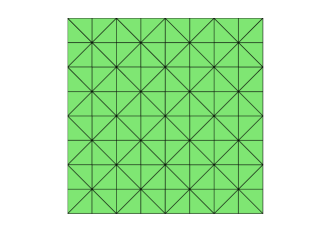
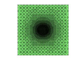
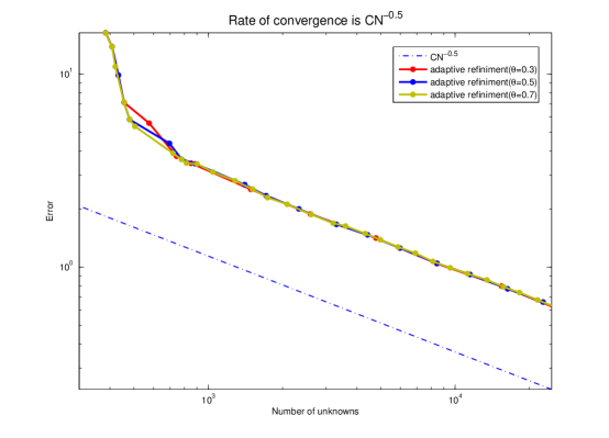
Figure 2 shows the rate of v.s. with different marking parameters and , where and represent the number of elements and the corresponding solution, respectively, gotten from the Algorithm 4.1.
Example 5.2.
In this example, we choose the L-shape domain and coefficient , the exact solution of (1.1) is .
On the left of Figure 3 shows the initial mesh for Example 5.2; on the right of Figure 3 shows the refined mesh after iterations for the Example 5.2 with .
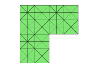
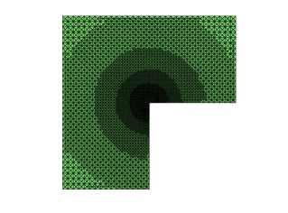
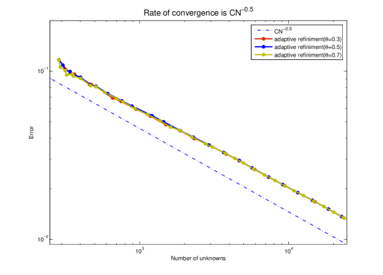
Figure 4 shows the rate of v.s. with different marking parameters and , where and represent the number of elements and the corresponding solution, respectively, gotten from the Algorithm 4.1.
References
- [1] A. Alonso. Error estimators for a mixed method. Numer. Math., 74(4):385–395, 1996.
- [2] D. N. Arnold. An interior penalty finite element method with discontinuous elements. SIAM J. Numer. Anal., 19(4):742–760, 1982.
- [3] B. Ayuso de Dios, K. Lipnikov, and G. Manzini. The nonconforming virtual element method. ESAIM: Mathematical Modelling and Numerical Analysis (M2AN), 50(3):879–904, 2016.
- [4] Betul Bogrek and Xiaoshen Wang. Superconvergence of a modified weak galerkin approximation for second order elliptic problems by l2 projection method. Journal of Computational and Applied Mathematics, 346:53–62, 2019.
- [5] A. Bonito and R. H. Nochetto. Quasi-optimal convergence rate of an adaptive discontinuous Galerkin method. SIAM J. Numer. Anal., 48(2):734–771, 2010.
- [6] Z. Q. Cai and S. H. Cao. A recovery-based a posteriori error estimator for interface problems. Computer Methods in Applied Mechanics and Engineering, 296(1):169–195, 2015.
- [7] Shuhao Cao, Chunmei Wang, and Junping Wang. A new numerical method for div-curl systems with low regularity assumptions. Computers & Mathematics with Applications, 114:47–59, 2022.
- [8] C. Carstensen, S. Bartels, and S. Jansche. A posteriori error estimates for nonconforming finite element methods. Numer. Math., 92(2):233–256, 2002.
- [9] J. M. Cascon, C. Kreuzer, R. H. Nochetto, and K. G. Siebert. Quasi-optimal convergence rate for an adaptive finite element method. SIAM J. Numer. Anal., 46(5):2524–2550, 2008.
- [10] L Chen. iFEM: an integrated finite element methods package in MATLAB. University of California at Irvine, 2009.
- [11] L. Chen, M. Holst, and J. C. Xu. Convergence and optimality of adaptive mixed finite element methods. Math. Comp., 78(265):35–53, 2009.
- [12] L. Chen, J. P. Wang, and X. Ye. A posteriori error estimates for weak Galerkin finite element methods for second order elliptic problems. J. Sci. Comput., 59(2):496–511, 2014.
- [13] Long Chen, Junping Wang, Yanqiu Wang, and Xiu Ye. An auxiliary space multigrid preconditioner for the weak galerkin method. Computers & Mathematics with Applications, 70(4):330–344, 2015.
- [14] Z. M. Chen and S. B. Dai. On the efficiency of adaptive finite element methods for elliptic problems with discontinuous coefficients. SIAM Journal on Scientific Computing, 24(2):443–462, 2002.
- [15] P. Ciarlet, C. F. Dunkl, and S. A. Sauter. A family of Crouzeix-Raviart finite elements in 3D. Analysis and Applications, 16(5):649–691, 2018.
- [16] P. G. Ciarlet. The Finite Element Method for Elliptic Problems, volume 4 of Studies in Mathematics and its Applications. North-Holland Publishing Co., 1978.
- [17] P. G. Ciarlet, P. Ciarlet, S. A. Sauter, and C. Simian. Intrinsic finite element methods for the computation of fluxes for Poisson’s equation. Numerische Mathematik, 132(3):433–462, 2016.
- [18] M. Crouzeix and P. A. Raviart. Conforming and nonconforming finite element methods for solving the stationary Stokes equations I. Revue française dautomatique informatique recherche opérationnelle. Mathématique, 7(R3):33–75, 1973.
- [19] Ming Cui, Xiu Ye, and Shangyou Zhang. A modified weak galerkin finite element method for the biharmonic equation on polytopal meshes. Communications on Applied Mathematics and Computation, 3(1):91–105, 2021.
- [20] E. Dari, R. Duran, C. Padra, and V. Vampa. A posteriori error estimators for nonconforming finite element methods. Mathematical Modelling and Numerical Analysis, 30(4):385–400, 1996.
- [21] W. Dörfler. A convergent adaptive algorithm for Poisson’s equation. SIAM Journal on Numerical Analysis, 33(3):1106–1124, 1996.
- [22] Y. Du and Z. M. Zhang. A numerical analysis of the weak Galerkin method for the Helmholtz equation with high wave number. Commun. Comput. Phys., 22(1):133–156, 2017.
- [23] F. Z. Gao and X. S. Wang. A modified weak galerkin finite element method for a class of parabolic problems. J. Comput. Appl. Math., 271(1):1–19, 2014.
- [24] V. Girault and P.-A. Raviart. Finite Element Methods for Navier-Stokes Equations: Theory and Algorithms. Springer-Verlag, 1986.
- [25] Liming Guo, Qiwei Sheng, Cheng Wang, and Ziping Huang. A modified weak galerkin finite element method for nonmonotone quasilinear elliptic problems. Journal of Computational and Applied Mathematics, 406:113928, 2022.
- [26] J. Hu and J. C. Xu. Convergence and optimality of the adaptive nonconforming linear element method for the stokes problem. J. Sci. Comput., 55(1):125–148, 2013.
- [27] X. Z. Hu, L. Mu, and X. Ye. A weak Galerkin finite element method for the Navier-Stokes equations. J. Comput. Appl. Math., 362:614–625, 2019.
- [28] J. G. Huang and Y. F. Xu. Convergence and complexity of arbitrary order adaptive mixed element methods for the Poisson equation. Sci. China Math., 55(5):1083–1098, 2012.
- [29] Saqib Hussain, Xiaoshen Wang, and Ahmed Al-Taweel. A study of mixed problem for second order elliptic problems using modified weak galerkin finite element method. Journal of Computational and Applied Mathematics, 401:113770, 2022.
- [30] Binjie Li and Xiaoping Xie. Bpx preconditioner for nonstandard finite element methods for diffusion problems. SIAM Journal on Numerical Analysis, 54(2):1147–1168, 2016.
- [31] Guanrong Li, Yanping Chen, and Yunqing Huang. A new weak galerkin finite element scheme for general second-order elliptic problems. Journal of Computational and Applied Mathematics, 344:701–715, 2018.
- [32] Guanrong Li, Yanping Chen, and Yunqing Huang. A robust modified weak galerkin finite element method for reaction-diffusion equations. Numer. Math. Theor. Meth. Appl, 15:68–90, 2022.
- [33] H.G. Li, L. Mu, and X. Ye. A posteriori error estimates for the weak Galerkin finite element methods on polytopal meshes. Comm. Comput. Phys., 26(2):558–578, 2019.
- [34] X. Liu, J. Li, and Z. X. Chen. A weak galerkin finite element method for the Navier-Stokes equations. J. Comp. Appl. Math., 333:442–457, 2018.
- [35] L. Mu. Weak Galerkin based a posteriori error estimates for second order elliptic interface problems on polygonal meshes. J. Comput. Appl. Math., 361:413–425, 2019.
- [36] L. Mu, J. P. Wang, Y. Q. Wang, and X. Ye. A computational study of the weak Galerkin method for second-order elliptic equations. Numer. Algorithms, 63(4):753–777, 2013.
- [37] L. Mu, J. P. Wang, G. W. Wei, and S. Zhao. Weak Galerkin methods for second order elliptic interface problems. Int. J. Numer. Anal. Model., 250:106–125, 2013.
- [38] L. Mu, J. P. Wang, and X. Ye. Weak Galerkin finite element methods for the biharmonic equation on polytopal meshes. Numer. Methods Partial Differential Equations, 30(3):1003–1029, 2014.
- [39] L. Mu, J. P. Wang, and X. Ye. A weak Galerkin finite element method with polynomial reduction. J. Comp. Appl. Math., 285:45–58, 2015.
- [40] L. Mu, J. P. Wang, and X. Ye. A new weak Galerkin finite element method for the Helmholtz equation. IMA J. Numer. Anal., 35(3):1228–1255, 2015.
- [41] L. Mu, J. P. Wang, and X. Ye. Weak Galerkin finite element methods on polytopal meshes. Int. J. Numer. Anal. Model., 12(1):31–53, 2015.
- [42] L. Mu, J. P. Wang, X. Ye, and S. Y. Zhang. A -weak Galerkin finite element method for the biharmonic equation. J. Sci. Comput., 30(3):473–495, 2014.
- [43] L. Mu, J. P. Wang, X. Ye, and S. Zhao. A numerical study on the weak Galerkin method for the Helmholtz equation. Commun. Comput. Phys., 15(5):1461–1479, 2014.
- [44] Lin Mu, Junping Wang, Xiu Ye, and Shangyou Zhang. A weak galerkin finite element method for the maxwell equations. Journal of Scientific Computing, 65(1):363–386, 2015.
- [45] R. H. Nochetto, K. G. Siebert, and A. Veeser. Multiscale, Nonlinear and Adaptive Approximation, chapter Theory of adaptive finite element methods: an introduction, pages 409–542. Springer, 2009.
- [46] L. Owens. Quasi-optimal convergence rate of an adaptive weakly over-penalized interior penalty method. J. Sci. Comput., 59(2):309–333, 2014.
- [47] M. Petzoldt. A posteriori error estimators for elliptic equations with discontinuous coefficients. Adv. Comput. Math., 16(1):47–75, 2002.
- [48] K. Shahbazi. An explicit expression for the penalty parameter of the interior penalty method. J. Comput. Phys., 205(2):401–407, 2005.
- [49] Sidney Shields, Jichun Li, and Eric A Machorro. Weak galerkin methods for time-dependent maxwell’s equations. Computers & Mathematics with Applications, 74(9):2106–2124, 2017.
- [50] M. Tang, L. Q. Zhong, and Y. Y. Xie. A modified weak Galerkin method for h(curl)-elliptic problem. Comput. Math. Appl., 2022.
- [51] T. Tian, Q. L. Zhai, and R. Zhang. A new modified weak Galerkin finite element scheme for solving the stationary Stokes equations. J. Comput. Appl. Math., 329:268–279, 2018.
- [52] R. Verfürth. A review of a posteriori error estimation and adaptive mesh refinement techniques. Wiley Teubner, Chichester and Newyork, 1996.
- [53] J. P. Wang and X. Ye. A weak Galerkin finite element method for second-order elliptic problems. J. Comp. Appl. Math., 241:103–115, 2013.
- [54] J. P. Wang and X. Ye. A weak Galerkin mixed finite element method for second order elliptic problems. Math. Comp., 83(289):2101–2126, 2014.
- [55] X. Wang, N. S. Malluwawadu, F. Gao, and T. C. McMillan. A modified weak Galerkin finite element method. J. Comput. Appl. Math., 271:319–327, 2014.
- [56] Xiuli Wang, Xianglong Meng, Shangyou Zhang, and Huifang Zhou. A modified weak galerkin finite element method for the linear elasticity problem in mixed form. Journal of Computational and Applied Mathematics, 420:114743, 2023.
- [57] Y. Y Xie, L. Q. Zhong, and Y. P. Zeng. Convergence of an adaptive modified WG method for second-order elliptic problem. Numer. Algorithms, 90(2):789–808, 2022.
- [58] Y. P. Zeng, J. R. Chen, and F. Wang. Convergence analysis of a modified weak Galerkin finite element method for Signorini and obstacle problems. Numer. Methods Partial Differential Equations, 33(5):1459–1474, 2017.
- [59] T. Zhang and Y. L. Chen. A posteriori error analysis for the weak Galerkin method for solving elliptic problems. Int. J. Comput. Methods, 15(8):1850075, 2018.
- [60] T. Zhang and T. Lin. A posteriori error estimate for a modified weak galerkin method solving elliptic problems. Numer. Methods for Partial Differential Equations, 33(1):381–398, 2017.
- [61] X. B. Zheng and X. P. Xie. A posteriori error estimator for a weak Galerkin finite element solution of the Stokes problem. East Asian Journal on Applied Mathematics, 7(3):508–529, 2017.