Graph Gamma Process Generalized Linear Dynamical Systems

Abstract

We introduce graph gamma process (GGP) linear dynamical systems to model real-valued multivariate time series. For temporal pattern discovery, the latent representation under the model is used to decompose the time series into a parsimonious set of multivariate sub-sequences. In each sub-sequence, different data dimensions often share similar temporal patterns but may exhibit distinct magnitudes, and hence allowing the superposition of all sub-sequences to exhibit diverse behaviors at different data dimensions. We further generalize the proposed model by replacing the Gaussian observation layer with the negative binomial distribution to model multivariate count time series. Generated from the proposed GGP is an infinite dimensional directed sparse random graph, which is constructed by taking the logical OR operation of countably infinite binary adjacency matrices that share the same set of countably infinite nodes. Each of these adjacency matrices is associated with a weight to indicate its activation strength, and places a finite number of edges between a finite subset of nodes belonging to the same node community. We use the generated random graph, whose number of nonzero-degree nodes is finite, to define both the sparsity pattern and dimension of the latent state transition matrix of a (generalized) linear dynamical system. The activation strength of each node community relative to the overall activation strength is used to extract a multivariate sub-sequence, revealing the data pattern captured by the corresponding community. On both synthetic and real-world time series, the proposed nonparametric Bayesian dynamic models, which are initialized at random, consistently exhibit good predictive performance in comparison to a variety of baseline models, revealing interpretable latent state transition patterns and decomposing the time series into distinctly behaved sub-sequences.

1 Introduction

Linear dynamical systems (LDSs) have been widely used to model real-valued time series (Kalman, 1960; West and Harrison, 1997; Ghahramani and Roweis, 1999; Ljung, 1999), with diverse applications such as financial time series analysis (Carvalho and Lopes, 2007) and movement trajectory modeling (Gao et al., 2016; Zhang et al., 2017). They have become standard tools in optimal filtering, smoothing, and control (Imani and Braga-Neto, 2018; Hardt et al., 2018; Koyama, 2018). An LDS consists of two main blocks, including an observation model, which assumes that the observations are translated from their latent states via a linear system with added Gaussian noise, and a transition block, which is represented by a Markov chain that linearly transforms a latent state from time $t-1$ to time $t$ with added Gaussian noise. The transition block plays an important role in capturing the underlying dynamics of the data. An LDS, which has limited representation power due to its linear assumption, allows one to examine the temporal trajectory of each latent dimension to understand the role played by the corresponding latent factor. While it is often considered to be simple to interpret, its interpretability often quickly deteriorates as its latent state dimension increases.

To enhance the representation power of LDSs, in particular, to model non-linear behaviors of the time series and improve their interpretability, one may consider switching LDSs (Fox et al., 2009; Linderman et al., 2017; Nassar et al., 2018), which learn how to divide the time series into separate temporal segments and fit them by switching between different LDSs. Important parameters include the number of different LDSs, their latent state dimensions, and the transition mechanism from one LDS to another. While nonparametric Bayesian techniques have been applied to switching LDSs to learn the number of LDSs that is needed, the latent state dimensions often stay as tuning parameters to be set (Fox et al., 2009; Nassar et al., 2018). Moreover, switching LDSs do not allow different LDSs to share latent states, making it difficult to capture smooth transitions between different temporal patterns, and false positives/negatives and delays in detecting the switching points will also compromise their performance. In addition, existing optimal smoothing and filtering techniques developed for LDSs, such as Kalman filtering (Kalman, 1960), require non-trivial modifications before being able to be applied to switching LDSs (Murphy, 1998).

Moving beyond switching LDSs where different LDSs neither share their latent states nor overlap in time, we propose the graph gamma process (GGP) LDS that encourages forming multiple LDSs that can share their latent states and co-occur at the same time. GGP-LDS uses a flexible combination of multiple LDSs to fit the observation at any given time point, allowing smooth transitions between different dynamical patterns across time. A notable feature of GGP-LDS is that existing optimal filtering and smoothing techniques developed for a canonical LDS can be readily applied to GGP-LDS without any modification. Therefore, GGP-LDS can serve as a plug-in replacement of the LDS in an existing system. The introduced nonparametric Bayesian construction in GGP-LDS will support $S$ latent states that are shared by $K$ different types of LDSs, each of which is characterized by its own pattern of activation probabilities imposed on a $S\times S$ sparse state-transition matrix, and allow both $S$ and $K$ to grow without bound. This unique construction is realized by modeling the sparsity structure of the $S\times S$ state-transition matrix as the adjacency matrix of a directed random graph, which is resulted from the logical OR operation over $K$ latent binary adjacency matrices, each of which is drawn according to the interaction strengths between the states (nodes) of a type of LDS (node community). Each latent binary adjacency matrix can be considered as a specific type of state community, which describes a particular type of relationship between latent states, $i.e.$, for a given state of the current time, which states of the previous states will directly influence it, and which states of the future time will be directly influenced by it. While a latent state is associated with all communities, the association strengths can clearly differ. Note that the sparsity pattern of the state-transition matrix is determined by the logical OR of these community-specific binary adjacency matrices. Therefore, to facilitate interpretation and visualization, one can hard assign a state to a community whose binary adjacency matrix best explains how this state is being influenced by the states of the previous time, or to a community that best explains how this state is influencing the states of the next time.

GGP-LDS allows approximating complex nonlinear dynamics by activating a certain combination of communities to model a particular type of linear dynamics at any given time, and using smooth transitions between overlapping communities to model smooth transitions between distinct linear dynamics. The characteristics of each community can be visualized by reconstructing the observations using the inferred latent representation and a community-specific reweighted latent state-transition matrix, where the weights are determined by the activation strength of that community relative to the combined activation strength of all communities. In addition to modeling real-valued time series, we show how to generalize the observation layer of GGP-LDS to model overdispersed count time series. It is noteworthy to mention that while the LDS (Kalman, 1963) has been chosen as the transition and observation model of GGP-LDS, the proposed GGP can potentially be applied to many other nonlinear systems that have a latent state transition module (Johnson et al., 2016).

2 Nonparametric Bayesian Modeling

For LDSs, let us denote $\bm{y}_{t}\in\mathbb{R}^{V}$ and $\bm{x}_{t}\in\mathbb{R}^{S}$ as the observed data and latent state vectors, respectively, at time $t\in\{1,\ldots,T\}$, ${\bf D}=(\bm{d}_{1},\ldots,\bm{d}_{S})\in\mathbb{R}^{V\times S}$ as the observation factor loading matrix, and both $\bm{\Phi}\in\mathbb{R}^{V\times V}$ and $\bm{\Lambda}=\mbox{diag}(\lambda_{1},\ldots,\lambda_{S})$ as precision (inverse covariance) matrices. Inspired by Kalantari et al. (2018), we first modify the usual LDS hierarchical model by utilizing a spike-and-slab construction (Mitchell and Beauchamp, 1988; Ishwaran and Rao, 2005; Zhou et al., 2009), which imposes binary mask ${\bf Z}\in\{0,1\}^{S\times S}$ element-wise on the real-valued latent state transition matrix ${{\bf W}}\in\mathbb{R}^{S\times S}$ as

$$\bm{y}_{t}\sim\mathcal{N}({\bf D}\bm{x}_{t},\bm{\Phi}^{-1}),~{}\bm{x}_{t}\sim\mathcal{N}\left(\left({{\bf W}}\odot{\bf Z}\right)\bm{x}_{t-1},\bm{\Lambda}^{-1}\right).$$

For count observations, we modify the Gaussian distribution based observation layer with the negative binomial (NB) distribution by letting $\small\bm{y}_{t}\sim\mbox{NB}\left(\eta,{\sigma({\bf D}\bm{x}_{t})}\right),~{}\eta\sim\mbox{Gamma}(\alpha_{\eta},1/\beta_{\eta}),~{}\bm{x}_{t}\sim\mathcal{N}\left(\left({{\bf W}}\odot{\bf Z}\right)\bm{x}_{t-1},\bm{\Lambda}^{-1}\right),$ where $\sigma(x):={1}/({1-e^{-x}})$ is the sigmoid function.

The $K\times K$ latent state-transition matrix ${{\bf W}}\odot{\bf Z}$, in particular, the sparsity structure of ${\bf Z}$, plays an important role in determining the dynamical behaviors of the model. First, the nonzero locations in ${\bf Z}$ determine the temporal dependencies between the latent states (Kalantari et al., 2018). For example, if $z_{ij}$, the $(i,j)$th element of ${\bf Z}$, is zero, then at time $t$, $x_{ti}$ will be independent of $x_{(t-1)j}$, and $x_{tj}$ will not influence $x_{(t+1)i}$. Thus in what follows, we consider that there is a directed link (edge) from states (nodes) $j$ to $i$ if $z_{ij}=1$.

Second, viewing ${\bf Z}$ as the adjacency matrix of a directed random graph and the states of the LDS as the graph nodes, we may introduce inductive bias to encourage its nodes to be formed into overlapping communities, reflected by overlapping dense blocks along the diagonal of the adjacency matrix after appropriately rearranging the orders of the nodes. We may then view each community as an LDS, which forms its own state-transition matrix, using a submatrix of ${{\bf W}}\odot{\bf Z}$, to model the transitions between the corresponding subset of states. This construction allows approximating complex nonlinear dynamics by activating different communities at different levels to model a particular type of linear dynamics at any given time, and using smooth transitions between overlapping communities to model the smooth transitions between distinct linear dynamics.

To induce the structure of overlapping communities into ${\bf Z}$, the adjacency matrix of a directed random graph, and allow both the number of communities and number of nodes (dimension of ${\bf Z}$) to grow without bound, we propose the graph gamma process (GGP). A draw from the GGP consists of countably infinite latent communities, each of which is associated with a positive weight indicating the overall activation strength of the community. These communities all share the same set of countably infinite nodes (states) but place different weights on how strongly a node is associated with a community. We describe the detail in what follows.

2.1 Graph Gamma Process

Denote $Z(i,:)$ and $Z(:,i)$ as row $i$ and column $i$ of ${\bf Z}$, respectively. Since $\mathbb{E}[\bm{x}_{t}\,|\,\bm{x}_{t-1},{{\bf W}},{\bf Z}]=({{\bf W}}\odot{\bf Z})\bm{x}_{t-1}$, we have

$$\mathbb{E}[x_{ti}\,|\,\bm{x}_{t-1},{{\bf W}},{\bf Z}]=(W(i,:)\odot Z(i,:))\bm{x}_{t-1},$$ (1)

$$\mathbb{E}[\bm{x}_{t+1}\,|\,\bm{x}_{t},{{\bf W}},{\bf Z}]=\textstyle(W(:,i)\odot Z(:,i))x_{ti}+\sum_{j\neq i}^{\infty}(W(:,j)\odot Z(:,j))x_{tj},$$ (2)

which means $x_{ti}$ will be dependent on $\bm{x}_{t-1}$ if ${Z(i,:)}$ contains non-zero elements, and it will influence $\bm{x}_{t+1}$ if $Z(:,i)$ contains non-zero elements. To construct a nonparametric Bayesian model that removes the need to tune the hidden state dimension, our first goal is to allow ${\bf Z}$ to have an unbounded number of rows and columns, which means that the model can support countably infinite state-specific factors $\bm{d}_{i}$, with which the mean of $\bm{y}_{t}$ given $\bm{x}_{t}$ is factorized as $\mathbb{E}[\bm{y}_{t}\,|\,\bm{x}_{t},{\bf D}]={\bf D}\bm{x}_{t}=\sum_{t=1}^{\infty}\bm{d}_{i}x_{ti}$.

To achieve this goal, with $c_{\rho}>0$ and $G_{0,\rho}$ defined as a finite and continuous base measure over a complete and separable metric space $\Omega$, we first introduce a gamma process $G_{\rho}\sim\Gamma\mbox{P}(c_{\rho},G_{0,\rho})$ on the product space $\mathbb{R}^{+}\times\Omega$, where $\mathbb{R}^{+}:=\{x:x>0\}$, such that for each subset $A\subset\Omega$, we have $G_{\rho}(A)\sim\mbox{Gamma}(G_{0,\rho}(A),1/c_{\rho})$. The Lévy measure of this gamma process can be expressed as $\nu(d\rho d\bm{d})=\rho^{-1}e^{-c_{\rho}\rho}d\rho G_{0,\rho}(d\bm{d})$. A draw from this gamma process can be expressed as $G_{\rho}=\sum_{i=1}^{\infty}\rho_{i}d\bm{d}_{i}$, consisting of countably infinite atoms (factors) $\bm{d}_{i}$ with weights $\rho_{i}$. We view $\bm{d}_{i}$ as the factor loading vector for latent state $i$, and will make $\rho_{i}$ determine the number of nonzero elements in $Z(i,:)$ and, consequently, how strongly $x_{ti}$, the activation of state $i$ at time $t$, is influenced by $\bm{x}_{t-1}$ of the previous time. As the number of $\rho_{i}$ that are larger than an arbitrarily small constant $\epsilon$ follows a Poisson distribution with a finite mean as $\gamma_{0,\rho}\int_{\epsilon}^{\infty}\rho^{-1}e^{-c_{\rho}\rho}d\rho$, where $\gamma_{0,\rho}:=G_{0,\rho}(\Omega)$ is the mass parameter, this can be used to express the idea that only a finite number of elements in $\{x_{ti}\}_{i=1,\infty}$ at time $t$ will be dependent on $\bm{x}_{t-1}$ of the previous time.

We further mark each $\rho_{i}$ with a degenerate gamma random variable, changing the Lévy measure of the gamma process to that of a marked gamma process (Kingman, 1993) as $\nu(d\rho\,d\bm{d}\,d\tau)=\rho^{-1}e^{-c_{\rho}\rho}d\rho G_{0,\rho}(d\bm{d})\gamma_{0,\tau}\tau^{-1}e^{-c_{\tau}\tau}d\tau$; we express a draw from this marked gamma process as $G_{\rho,\tau}=\sum_{i=1}^{\infty}{(\rho_{i},\tau_{i})\delta_{\bm{d}_{i}}}$. We will make $\tau_{i}$ determine the random number of nonzero elements in $Z(:,i)$ and, consequently, how strongly $x_{ti}$, the factor score of state $i$ at time $t$, will influence $\bm{x}_{t+1}$ of the next time point. As the number of $\tau_{i}$ that are larger than an arbitrarily small constant $\epsilon$ follows a Poisson distribution with a finite mean as $\gamma_{0,\tau}\int_{\epsilon}^{\infty}\tau^{-1}e^{-c_{\tau}\tau}d\tau$, this can be used to express the idea that only a finite number elements in $\{x_{ti}\}_{i=1,\infty}$ at time $t$ will influence $\bm{x}_{t+1}$.

Given $G_{\rho,\tau}=\sum_{i=1}^{\infty}{(\rho_{i},\tau_{i})\delta_{\bm{d}_{i}}}$, we further define a gamma process $G_{o}\sim\Gamma\mbox{P}(c_{o},G_{\rho,\tau})$, with Lévy measure $\nu(drd\bm{\theta}d\bm{\psi})=r^{-1}e^{-cr}drG_{o}(d\bm{\theta}d\bm{\psi})$, a draw from which is expressed as $G_{o}=\sum_{\kappa=1}^{\infty}r_{\kappa}\delta_{\{\bm{\theta}_{\kappa},\bm{\psi}_{\kappa}\}}$. In this random draw, $r_{\kappa}\in\mathbb{R}_{+}$, reflecting the activation strength of community $\kappa$, is the weight of the $\kappa$th atom $\{\bm{\theta}_{\kappa},\bm{\psi}_{\kappa}\}$, where $\bm{\theta}_{\kappa}=(\theta_{1\kappa},\ldots,\theta_{\infty\kappa})^{T}$, $\bm{\psi}_{\kappa}=(\psi_{1\kappa},\ldots,\psi_{\infty\kappa})^{T}$, and $\theta_{i\kappa}$ and $\psi_{i\kappa}$, representing how strongly that node $i$ is associated with community $\kappa$, are defined on $\rho_{i}$ and $\tau_{i}$, the weights of the atoms of the gamma process $G_{\rho,\tau}$, using

$$\theta_{i\kappa}\sim\mbox{Gamma}(\rho_{i},1/e),~{}~{}\psi_{i\kappa}\sim\mbox{Gamma}(\tau_{i},1/f).$$

We refer to the hierarchical stochastic process constructed in this way as the GGP. We denote the mass parameter of the GGP as $\gamma_{0}:=\int G_{o}(d\bm{\theta}d\bm{\psi})$. Inherited from the property of a gamma process, the GGP has an inherent shrinkage mechanism that its number of atoms (node communities) with weights greater than $\epsilon>0$ is a finite random number drawn from $\mbox{Pois}(\gamma_{0}\int_{\epsilon}^{\infty}{r^{-1}e^{-cr}dr})$.

Given a random draw from the GGP as $G_{o}=\sum_{\kappa=1}^{\infty}r_{\kappa}\delta_{\{\bm{\theta}_{\kappa},\bm{\psi}_{\kappa}\}},$ we will let $r_{\kappa}$ determine the overall activation strength of community $\kappa$, $\theta_{i\kappa}$ how strongly state $i$ in community $\kappa$ is influenced by the states of the previous time in the same community, and $\psi_{j\kappa}$ how strongly state $j$ in community $\kappa$ influences the states of the next time in the same community. To express this idea, for community $\kappa$ parameterized by $\{r_{\kappa},\bm{\theta}_{\kappa},\bm{\psi}_{\kappa}\}$, we generate a community-specific sparse adjacency matrix, whose $(i,j)$th element is drawn as

$$z_{ij\kappa}\sim\mbox{Bernoulli}(1-e^{-r_{\kappa}\theta_{i{\kappa}}\psi_{j{\kappa}}}).$$ (3)

Thus from nodes $j$ to $i$, community $\kappa$ defines its own interaction probability, expressed as $p_{ij\kappa}=1-e^{-r_{\kappa}\theta_{i{\kappa}}\psi_{j{\kappa}}}$, and draws a binary edge $z_{ij\kappa}$ based on $p_{ij\kappa}$. While there are countably infinite nodes, in community $\kappa$, the total number of edges is a finite random number and hence the number of nodes with nonzero degrees is also finite.

Lemma 1.

The number of edges in community $\kappa$, expressed as $\sum_{i=1}^{\infty}\sum_{j=1}^{\infty}z_{ij\kappa}$, is finite.

As in (3), whether $z_{ij\kappa}=1$ or 0 is related to both the overall strength of community $\kappa$ and how strongly nodes $i$ and $j$ are affiliated with community $\kappa$. Lemma 1, whose proof is deferred to the Appendix, suggests that we can extract a finite submatrix $\mathcal{Z}_{\kappa}:=\{z_{ij\kappa}\}_{i,j\in\mathcal{S}_{\kappa}}$, where $\textstyle\mathcal{S}_{\kappa}:=\{i:\sum_{j}z_{ij\kappa}+\sum_{j}z_{ji\kappa}>0\}$ is the set of nodes with non-zero degrees in community $\kappa$. We consider $\mathcal{S}_{\kappa}$ as the nodes activated by community $\kappa$ and $\mathcal{Z}_{\kappa}$ as its nonempty graph adjacency matrix. Thus under the proposed GGP construction, different communities could overlap in the nodes belonging to their respective nonempty graph adjacency matrices, which means it is possible that $\mathcal{S}_{\kappa}\cap\mathcal{S}_{\kappa^{\prime}}\neq\emptyset$ for $\kappa\neq\kappa^{\prime}$. If $\mathcal{S}_{\kappa}\cap\mathcal{S}_{\kappa^{\prime}}=\emptyset$, then we consider communities $\kappa$ and $\kappa^{\prime}$ as two non-overlapping communities.

Our previous analysis tells that whether $z_{ij}=1$ determines not only whether state $i$ at a given time will be dependent of the states of the previous time, but also whether state $j$ at a given time will influence the states of the next time. To express the idea that whether $z_{ij}=1$ is collectively decided by all countably infinite communities, whose nonempty adjacency matrices could overlap in their selections of nodes, we take the OR operation over all elements in $\{z_{ij\kappa}\}_{\kappa}$ to define the adjacency matrix of the full model as

$$z_{ij}=\lor_{\kappa=1}^{\infty}z_{ij\kappa},\vspace{0mm}$$ (4)

which means $z_{ij}=1$ if at least one $z_{ij\kappa}=1$, indicating community $\kappa$ places a directed edge from nodes $j$ to $i$, and $z_{ij}=0$ otherwise. In a matrix format, we have

$${\bf Z}=\lor_{\kappa=1}^{\infty}{\bf Z}^{(\kappa)},$$

where ${\bf Z}^{(\kappa)}$ represents the graph adjacency matrix of community $\kappa$, whose $(i,j)$th element is $z_{ij\kappa}$.

We note that marginalizing out $\{z_{ij\kappa}\}_{\kappa}$, we can directly draw the graph adjacency matrix defined in (4) as

$${\bf Z}\sim\mbox{Bernoulli}(1-e^{-\sum_{\kappa=1}^{\infty}r_{\kappa}\bm{\theta}_{k}\bm{\psi}_{k}^{T}}),$$ (5)

which can also be equivalently generated under the Bernoulli-Poisson link (Zhou, 2015) as

$$\textstyle{\bf Z}=\delta({\bf M}\geq 1),~{}{\bf M}=\sum_{\kappa=1}^{\infty}{\bf M}_{\kappa},~{}{\bf M}_{\kappa}\sim\mbox{Pois}(r_{\kappa}\bm{\theta}_{\kappa}\bm{\psi}_{\kappa}^{T}),$$

where $\delta(\bm{\cdot})$ returns one if the condition is true and zero otherwise. While the graph defined by ${\bf Z}$ has countably infinite nodes, the total number of edges is finite and hence the number of nodes with nonzero degrees is also finite; the proof of the following Lemma is deferred to the Appendix.

Lemma 2.

The number of edges in ${\bf Z}$, expressed as $\sum_{i=1}^{\infty}\sum_{j=1}^{\infty}z_{ij}$, is finite.

In summary, the GGP uses a gamma process to support countably infinite node communities in the prior, and another marked gamma process to support countably infinite number of nodes (states) shared by these communities. The adjacency matrix of the generated random graph from the GGP can be either viewed as taking the OR operation over all community-specific binary adjacency matrices, or viewed as thresholding a latent count matrix that aggregates the activation strengths across all communities for each node pair. Under this model construction, with the inherent shrinkage mechanisms of the gamma processes, only a finite number of communities will contain edges between the nodes, and the nonempty communities overlap with each other on their selections of nonzero-degree nodes, the total number of which across all communities is finite.

2.2 Overlapping Community based Model Interpretation and Visualization

As in (5), the sparsity pattern ${\bf Z}$ of the latent state-transition matrix can be linked to a latent count matrix whose expectation is $\sum_{\kappa}r_{\kappa}\bm{\theta}_{\kappa}\bm{\psi}_{\kappa}^{T}$. Thus we can measure the activation strength of community $k$ relative to the combined activation strength of all communities using

$$\mbox{{{\bf A}}}_{\kappa}:=\frac{r_{\kappa}\bm{\theta}_{\kappa}\bm{\psi}_{\kappa}^{T}}{\sum_{\kappa^{\prime}=1}^{K}r_{\kappa^{\prime}}\bm{\theta}_{\kappa^{\prime}}\bm{\psi}_{\kappa^{\prime}}^{T}}.$$ (6)

Due to the shrinkage property of the gamma process, only a small number of $r_{\kappa}$ are encourage to have non-negligible values. Therefore, there is often only a parsimonious set of active communities in the posterior. Since $\sum_{\kappa}{{\bf A}}_{\kappa}$ is a matrix whose elements are all equal to one, we can use the ${{\bf A}}_{\kappa}$’s to decompose the reconstruction of the time series under the proposed GGP-LDS into different sub-sequences, the $\kappa^{th}$ of which reveals the type of temporal patters captured by community $\kappa$.

More specifically, given the model parameters and latent state representation $\{\bm{x}_{t}\}_{t}$, taken from a posterior sample inferred by GGP-LDS, we define

$$\hat{\bm{y}}_{t}^{(\kappa)}={\bf D}\hat{\bm{x}}_{t}^{(\kappa)},~{}~{}\hat{\bm{x}}_{t}^{(\kappa)}=[({{\bf W}}\odot{\bf Z})\odot{{\bf A}}_{\kappa}]\bm{x}_{t-1}.$$ (7)

Note we have $\mathbb{E}[\bm{x}_{t}\,|\,{{\bf W}},{\bf Z},\bm{x}_{t-1}]=\sum_{\kappa}\hat{\bm{x}}_{t}^{(\kappa)}$ and $\mathbb{E}[\bm{y}_{t}\,|\,{\bf D},{{\bf W}},{\bf Z},\bm{x}_{t-1}]=\sum_{\kappa}\hat{\bm{y}}_{t}^{(\kappa)}$. Thus we can consider $\hat{\bm{y}}_{1:T}^{(\kappa)}$ as a sub-sequence in the data space and $\hat{\bm{x}}_{1:T}^{(\kappa)}$ as a sub-sequence in the latent space, both extracted according to the relative strength of community $\kappa$. Our experiments show that different dimensions of sub-sequence $\hat{\bm{y}}_{t}^{(\kappa)}$ often resemble each other in temporal patterns, but differ from each other in magnitudes, which is the reason why the aggregation of these sub-sequences, expressed as $\sum_{\kappa}\hat{\bm{y}}_{t}^{(\kappa)}$, can exhibit distinct temporal behaviors at different data dimensions. Note one may also define $\hat{\bm{x}}_{t}^{(\kappa)}=({{\bf W}}\odot{\bf Z}^{(\kappa)})\bm{x}_{t-1}$, which would lead to somewhat different community-specific sub-sequences, whose superposition no longer reconstructs $\mathbb{E}[\bm{y}_{t}\,|\,{\bf D},{{\bf W}},{\bf Z},\bm{x}_{t-1}]$ but may help highlight transitional time points between different linear dynamics.

To visualize the overlapping community structure of the latent states inferred by the proposed GGP-(G)LDS, we order the communities in decreasing oder based on their overall activation strength, which, for example, can be measured by either $\|{\bf Z}_{\kappa}\|_{0}=\sum_{i}\sum_{j}z_{ij\kappa}$ or $\|{\bf M}_{\kappa}\|_{1}=\sum_{i}\sum_{j}m_{ij\kappa}$. In this paper, we rank the activation strength according to $\|{\bf M}_{\kappa}\|_{1}$. As in (1), $Z(i,:)$ determines how latent state $i$ at the current time is influenced by the latent states of the previous time, and $Z(i,:)$ can be generated by thresholding latent counts $M(i,:)=\sum_{\kappa}M_{\kappa}(i,:)$. Thus we can we map row $i$ to community

$$\pi_{row}(i)=\textstyle\arg\max_{\kappa}\sum_{j}m_{ij\kappa},$$

the primary community via which latent state $i$ is influenced by the latent states of the previous time. Similarly, as in (2), $Z(:,j)$ determines how latent state $j$ at the current time is influencing the latent states of the next time, we can map column $j$ to community

$$\pi_{col}(j)=\textstyle\arg\max_{\kappa}\sum_{i}m_{ij\kappa},$$

the primarily community via which latent state $j$ influences the the latent states of the next time. To help visualize ${\bf Z}$, we rearrange its rows such that the rows mapped to the same community according to $\pi_{row}(i)$ are placed in the same row block, and we rearrange the columns in the same way according to $\pi_{col}(j)$.

For the rows inside the same row block ($i.e.$, sharing the same $\pi_{row}(i)$), we rearrange them in decreasing order based on $\sum_{j}m_{ij\pi_{row}(i)}$; we follow the same way to rearrange the columns inside each column block according to $\sum_{i}m_{ij\pi_{col}(j)}$.

Note that $m_{ij\kappa}$ are augmented count variables in a posterior sample, which are introduced to provide closed-form Gibbs sampling update equations, as described below.

2.3 Hierarchical Model and Bayesian Inference

To facilitate implementation, we truncate the GGP by setting $K$ as an upper-bound of the number of communities, and $S$ as an upper-bound of the number of states (nodes). We set $\gamma_{0,\rho}=\gamma_{0,\tau}=\gamma_{0}$. We make the scales of $\theta_{i\kappa}$ and $\psi_{j\kappa}$ change with $\kappa$ to increase model flexibility. The hierarchical model of the truncated GGP-LDS is expressed as

$$\bm{y}_{t}\sim\mathcal{N}({\bf D}\bm{x}_{t},\,\bm{\Phi}^{-1}),~{}\quad\mathbb{\Phi}\sim\mbox{Wishart}(\mathbb{V},V+2),$$

$$\bm{x}_{t}\sim\mathcal{N}\left[(\mathbb{W}\odot\mathbb{Z})\bm{x}_{t-1},\,\mbox{diag}(\lambda_{1},\ldots,\lambda_{S})^{-1}\right],$$

$$\bm{d}_{s}\sim\mathcal{N}\left(\mathbf{0},\,\mathbb{I}_{V}/\sqrt{V}\right),\quad\lambda_{s}\sim\mbox{Gamma}\left(a,1/b\right),$$

$$w_{ij}\sim\mathcal{N}(0,\varphi_{ij}^{-1}),\quad\varphi_{ij}\sim\mbox{Gamma}\left(\alpha_{0},{1}/{\beta_{0}}\right),$$

$$z_{ij}=\lor_{\kappa=1}^{K}z_{ij\kappa},\quad z_{ij\kappa}=\delta(m_{ij\kappa}\geq 1),$$

$$m_{ij\kappa}\sim\mbox{Pois}\left(r_{\kappa}\theta_{i\kappa}\psi_{j\kappa}\right),~{}\quad r_{\kappa}\sim\mbox{Gamma}({\gamma_{0}}/{K},{1}/{c}),$$

$$\theta_{i\kappa}\sim\mbox{Gamma}\left(\rho_{i},1/e_{\kappa}\right),\quad\rho_{i}\sim\mbox{Gamma}\left(\gamma_{0}/S,1/c_{\rho}\right),$$

$$\psi_{j\kappa}\sim\mbox{Gamma}\left(\tau_{j},1/f_{\kappa}\right),\quad\tau_{j}\sim\mbox{Gamma}\left(\gamma_{0}/S,1/c_{\tau}\right),$$ (8)

where $e_{\kappa},f_{\kappa}\sim\mbox{Gamma}\left(\alpha_{0},1/\beta_{0}\right)$ and ${\bm{x}_{0}}\sim\mathcal{N}({\bm{m}}_{0},{{\bf H}}_{0})$. As in Lemma 2, the total number of nonzero elements in ${\bf Z}$ has a finite expectation. Thus if the GGP truncation levels $K$ and $S$ are set large enough, it is expected for some state $i$ that $\sum_{j}z_{ij}=0$, which means its corresponding row in ${\bf Z}$ has no nonzero elements, and/or $\sum_{j}z_{ji}=0$, which means its corresponding column in ${\bf Z}$ has no nonzero elements. If node $i$ has zero degree that $\sum_{j}z_{ij}=\sum_{j}z_{ji}=0$, then $x_{ti}$ will neither be dependent on $\bm{x}_{t-1}$ nor influence $\bm{x}_{t+1}$, which means $\{x_{ti}\}_{t}$, the factor scores of state $i$, capture only the non-dynamic noise component of the data. Moreover, the proposed model will penalize the total energy captured by zero-degree node (state) $i$, expressed as $\sum_{t=1}^{T}x^{2}_{ti}$ if it is a zero-degree node (see Appendix B for more details).

To accommodate count data that are often overdispersed, we replace the Gaussian distribution based observation layer of GGP-LDS, $i.e.$, the first row of (8), with a negative binomial distribution based observation layer as

$$\bm{y}_{t}\sim\mbox{NB}\left(\eta,\sigma\left({\bf D}\bm{x}_{t}\right)\right),~{}\quad\eta\sim\mbox{Gamma}\left(\alpha_{\eta},1/\beta_{\eta}\right),\quad\alpha_{\eta},\beta_{\eta}\sim\mbox{Gamma}\left(\alpha_{0},1/\beta_{0}\right),$$ (9)

while keeping the other parts of the model unchanged; we refer to the modified model for count observation as GGP generalized LDS (GGP-GLDS). Due to the use of the negative binomial distribution, we may also refer to the modified model as GGP negative binomial dynamical system (GGP-NBDS).

We perform Bayesian inference via Gibbs sampling. Exploiting a variety of data augmentation and marginalization techniques developed for discrete data (Zhou and Carin, 2013; Zhou, 2015) , we provide closed-form Gibbs sampling updated equations for all model parameters, as described in detail in Appendix C. Unless specified otherwise, we consider 6000 Gibbs sampling iterations, treat the first 3000 samples as burnin, and collect one sample per 60 iterations afterwards, resulting in a collection of 50 posterior MCMC samples that are used to predict the means and uncertainty of future observations. In the following section, we provide a review of related work, where we compare the proposed models against a variety of dynamical systems, including switching LDSs and autoregressive, nonparametric, and deep neural network based models.

3 Related Work

The main challenges for modeling time series include providing accurate forecast, having the ability to process missing data, and learning interpretable latent representation such that latent structures ($e.g.$, clusters) can be translated into meaningful data temporal patterns, representing different time series behaviors, without the need to perform data specific tuning. A time series method addressing all these challenges is desired to have the following properties: 1) The underlying model is neither over- nor under-parameterized, which will result in over- or under-fitting, respectively, and hence poor performance in forecasting (Liu and Hauskrecht, 2015; Kalantari et al., 2018). 2) The model learns a parsimonious set of latent states such that the induced latent structures can explain the underlying patterns of the time series without the need of manual tuning. Inducing too many (overlapping) clusters of the latent states makes the model difficult to interpret, while imposing heavy regularization can enhance interpretability but hinder prediction. A good model will be able to balance interpretability and predictive performance. 3) The model is capable of modeling non-linear dynamics exhibited by the time series. 4) The model is capable of capturing latent state transition behaviors and the uncertainty of latent parameters. In this section, we review related works and discuss whether they satisfy the aforementioned properties.

Different from LDSs that employ latent state-transition blocks, autoregressive models that directly regress on the past observations are also commonly used to model real-valued time series data (Harrison et al., 2003; Davis et al., 2016; Saad and Mansinghka, 2018), with a wide range of applications, such as health care and epidemic modeling (Li et al., 2010; Kennedy and Turley, 2011). In addition to LDSs and autoregressive models, there also exist several other types of parametric models (Barber et al., 2011). To achieve good performance on a given time series, these parametric models in general require searching over a large set of possible parameter settings or model configurations via cross validation, or appropriately regularizing the training.

A variety of regularization techniques have been proposed for parameteric time series models. Charles et al. (2011) introduce a sparsity constraint on the update equations of Kalman filtering to enforce the latent state vectors to be sparse, but need to assume that all the other model parameters, including the observation and transition matrices and noise covariance matrices, are known. Städler et al. (2013) encourage a hidden Markov model (HMM) to have sparse state-specific inverse covariance matrices by imposing $L_{1}$-penalties on their elements. Liu and Hauskrecht (2015) propose to regularize the state transition matrix by penalizing its nuclear norm and imposing multivariate Laplacian priors over its rows. Siddiqi et al. (2010) propose a solution on reduced-rank HMM by relaxing the assumptions of a spectral learning algorithm by learning a $K$-dimensional subspace and finding the mapping between the high dimensional and low dimensional spaces.

Another set of time-series models are nonparametric Bayesian switching LDSs (Fox et al., 2009; Linderman et al., 2017), in which every temporal segment of the time series is fitted by one LDS. These models are focused on finding a mixture of LDSs, which are used to fit different time series segments, and a switching mechanism between different LDSs is learned to model the transitions between segments. Switching LDSs, however, may not provide satisfactory predictive performance on test data, as false switching, missed switching, and delayed switching could all compromise their predictions. Chiuso and Pillonetto (2010) design another type of nonparametric Bayesian models that identify sparse linear systems. Unlike the proposed GGP-LDS, it assumes no latent state transitions and models each observation as a linear combination of previous observations and some external input.

In addition, there are models that use the hierarchical Dirichlet process (Teh et al., 2006) priors over the states in hidden Markov models (Johnson and Willsky, 2013; Fox et al., 2009). There are also models that perform clustering on the time series use a Pitman-Yor process based mixture prior on non-linear state-space models (Nieto-Barajas et al., 2014), and Dirichlet process mixtures (Caron et al., 2008) for modeling noise distributions. These models are not fully nonparametric as they typically have some parametric assumptions as part of the model such as having a fixed number of hidden states or imposing explicit specifications of the underlying temporal dynamics, such as seasonality and trends.

Chiuso and Pillonetto (2010) design a nonparametric Bayesian model to identify sparse linear systems. It assumes no latent transitions and believes each observation is a linear combination of previous observations plus some external input. Saad and Mansinghka (2018) introduce a recurrent Chinese restaurant process based mixture to capture temporal dependencies and a hierarchical prior to discover groups of time series whose underlying dynamics are modeled jointly. This model is able to cluster the observations to a set of trajectories with similar behaviors, although it is prone to creating unnecessary clusters as if the same pattern repeats with different magnitudes in two different segments of the observation, these two segments are likely to be assigned to two different clusters. This may result in many unnecessary clusters for high dimensional and/or lengthy data.

Another widely used type of time series models are autoregressive models (Harrison et al., 2003; Davis et al., 2016; Saad and Mansinghka, 2018). There also exist several other parametric models, such as Barber et al. (2011), that provide additional tools to model time series. Most of these parametric models require searching over a large set of possible parameter settings with cross validation or model configurations to achieve satisfactory performance.

On the other side of the spectrum, we have a set of neural network based solutions, such as recurrent neural network based systems (Flunkert et al., 2017; Lai et al., 2018), which are quite flexible but suffer from several major limitations. They often provide point estimate of their parameters, without uncertainty estimation, and often have the problem of interpretability and need considerable amount of data to reliably train the model.

In this paper, we introduce a nonparametric Bayesian hierarchical model to address the aforementioned challenges. The proposed model is based on the LDS and GGP. The proposed GGP is designed to learn overlapping communities of latent states such that each community models a behavior which can be described with a linear system. Instead of assigning one community (LDS) to one segment of the observed trajectory, our model allows multiple communities to be used at any time point. This allows the model to break the sophisticated behavior in a trajectory to a weighted combination of simpler behaviors modeled by different linear systems, and it helps to model the nonlinearities of the data using multiple linear systems and smooth transitions between them.

4 Experimental Results

The code is provided at: https://github.com/GGPGLDS/GGP_GLDS. In this section, we will demonstrate the interpretablity of GGP-(G)LDS and its predictive performance on several different datasets. Due to the inherent shrinkage mechanisms of the GGP, we find that the proposed nonparametric Bayesian model is not sensitive to the choice of the truncation levels $S$ and $K$ as long as they are set large enough. For all the datasets in this section, we truncate them at $K=16$ and $S=30$, which are found to be large enough to accommodate all nonempty node communities, with interpretable latent representation and good predictive performance. Our Gibbs sampling based inference is not sensitive to initialization, allowing us to randomly initialize the model parameters. In this paper, we set $\gamma_{0}=\alpha_{0}=\beta_{0}=c=c_{\rho}=c_{\tau}=1$ for all experiments. We set $a=1$ and $b=0.1$ for all experiments (except for all visualizations, we set $b=1$ to encourage sparser latent state-transition matrices), encouraging $\lambda_{s}^{-1}$ to be small and hence encouraging the latent state representation vector to be constituted more by the autoregressive components and less by the white noise, generated by $\mathcal{N}\left[\mathbb{0},\mbox{diag}(\lambda_{1},\ldots,\lambda_{S})^{-1}\right]$.

For GGP-(G)LDS, we measure the performance of $t$-step prediction, for $t=1,\ldots,10$. In addition, 1-step-at-a-time predictive performance will be provided by using Kalman filter to update the state $\bm{x}_{t}$ after observing $\bm{y}_{t}$, while other model parameters, including ${\bf D}$, $\bm{\Phi}$, ${{\bf W}}$, ${\bf Z}$, and ${\bm{\lambda}}$, stay the same to make the next step prediction. Note that 1-step-at-a-time prediction via Kalman filter is only an option readily available for an LDS based system (not including switching LDS). Denoting $\hat{\bm{y}}_{t}$ as the $t$-step prediction of a given model, we measure its $t$-step predictive performance using mean absolute error (MAE) for real time series as

$$\mbox{MAE}_{t}=\sum_{v=1}^{V}\left|y_{dt}-\hat{y}_{dt}\right|/{V},$$ (10)

and use mean absolute relative error (MARE) for count time series as

$$\mbox{MARE}_{t}=\sum_{v=1}^{V}\frac{\left|y_{dt}-\hat{y}_{dt}\right|}{{V(y_{dt}+1)}}.$$ (11)

We compare the predictive performance of GGP-GLDS with these of several representative time series models, whose description and parameter setup for each dataset are described in detail below. For each dataset, we consider tuning important parameters for each competing algorithm. Notably for GGP-(G)LDS, when evaluating predictive performance, we simply use a same set of non-informative hyperparameters across all datasets and initialize all learnable parameters at random. Additional experiments on a synthetic dataset (the FitzHugh-Nagumo model) and a real dataset (closing stock price of twelve companies) will also be provided in the Appendix.

4.1 Lorenz Attractor

To demonstrate the performance of GGP-LDS on a dataset that has an underlying nonlinear dynamical pattern, we consider the Lorenz Attractor. We show how GGP-LDS finds an interpretable approximation to the generated time series with nonlinear dynamics. The Lorenz system is a classical nonlinear differential equation with three independent variables, defined as

$$\frac{dx_{1}}{dt}=\alpha(x_{2}-x_{1}),~{}~{}\ \frac{dx_{2}}{dt}=x_{1}(\beta-x_{3})-x_{2},~{}~{}\frac{dx_{3}}{dt}=x_{1}x_{2}-\gamma x_{3}.$$

There exist approximate solutions for this differential equation (Hernandez et al., 2018; Linderman et al., 2017; Nassar et al., 2018). A linear approximation will be very useful as we can leverage for this non-linear system many canonical algorithms developed for filtering and smoothing on linear systems. To show how our model approximates the latent states, we generate numerical solutions of the Lorenz system with a randomly generated initial state, $\alpha=1$, $\beta=2$, $\gamma=1$, and $T=578$ time points. The original generated variables under the Lorenz system have three dimensions ($x_{1},x_{2}$, and $x_{3}$). We treat them as latent variables and use a randomly generated $10\times 3$ matrix to map them to a 10-dimensional observation space. We use this $10\times T$ observed data with added white Gaussian noise to train both GGP-LDS and a variety of baseline models.

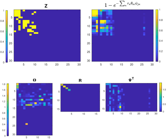
(a)

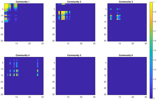
(b)

Figure 1: (a): Visualization of a GGP-LDS inferred posteriori sample on a Lorenz Attractor synthesized time series. Top Left: ${\bf Z}$ from this posterior sample, where the rows and columns are separately reordered with the method described in Section 2.2; Top Right: The inferred activation probability of ${\bf Z}$; Bottom Left: $\bm{\Theta}$, where $\theta_{i\kappa}$ shows how strongly state $i$ is influenced by the states of the previous time due to its association with community $\kappa$; Bottom Middle: ${\bf R}$, whose diagonal elements show the activation strength of different communities; Bottom Right: $\bm{\Psi}^{T}$, where $\psi_{\kappa,j}$ shows how strongly state $j$ influences the states of the next time due to its association with community $\kappa$.
   (b): Relative activation strength ${{\bf A}}_{\kappa}$, as defined in (6), of the top six communities; note that $4$ active communities formed over $15$ active latent states are inferred by GGP-LDS while the truncation levels of the GGP are set as $K=16$ and $S=30$.

Fig. 1(a) illustrates a single posterior sample of GGP-LDS, focusing on the inferred graph adjacency matrix, and the underlying activation probabilities of the edges of the graph adjacency matrix. More specifically, in the top row, we show on the left the graph adjacency matrix ${\bf Z}$, whose rows and columns have been separately reordered following the description in Section 2.2, and on the right the underlying edge activation probabilities. In the bottom row, we show $\bm{\Theta}=(\bm{\theta}_{1},\ldots,\bm{\theta}_{K})\in\mathbb{R}_{+}^{S\times K}$, ${\bf R}=\mbox{diag}(r_{1},\ldots,r_{K})\in\mathbb{R}_{+}^{K\times K}$, and $\bm{\Psi}^{T}=(\bm{\psi}_{1},\ldots,\bm{\psi}_{K})^{T}\in\mathbb{R}_{+}^{K\times S}$, where $\theta_{i\kappa}$ shows the affiliation strength of $x_{(t+1)i}$ to the $\kappa^{th}$ community ($\kappa^{th}$ LDS) and $\psi_{\kappa,j}$ shows the association strength of $x_{tj}$ to the $\kappa^{th}$ LDS.

It can be observed how the shrinkage property of the gamma process $G_{\rho,\tau}$ has been effective in sparsifying the rows of $\bm{\Theta}$ and columns of $\bm{\Psi}^{T}$, with unnecessary elements being shrunk towards zero. In addition, it can be seen that each active row of $\bm{\Theta}$, or active column of $\bm{\Psi}^{T}$ can potentially be a member of several different communities. The shrinkage property of the GGP $G_{o}$ drives many elements of $r_{k}$ towards zero and hence helps the model to pick which types of LDSs to be utilized. This is equivalent to say that the model infers which of these associations should be amplified or suppressed in expressing the underlying dynamics of the data. Moreover, for the $\bm{\Theta}$ matrix, it has 7 members (rows) associated with community one, which implies there are 7 corresponding states at time $t+1$ that will be influenced by $\bm{x}_{t}$ of the previous time due to their associations with community one, and $\bm{\Psi}^{T}$ shows that it has 4 members (columns) associated with community one, which implies that there are 4 corresponding states at time $t$ that will influence $\bm{x}_{t+1}$ of the next time due to their associations with community one. Thus the transition matrix of the first member of overlapping LDSs will be the $7\times 4$ block shown on the top left corner, as shown in both ${\bf Z}$ and its corresponding probability matrix in Fig. 1(a).

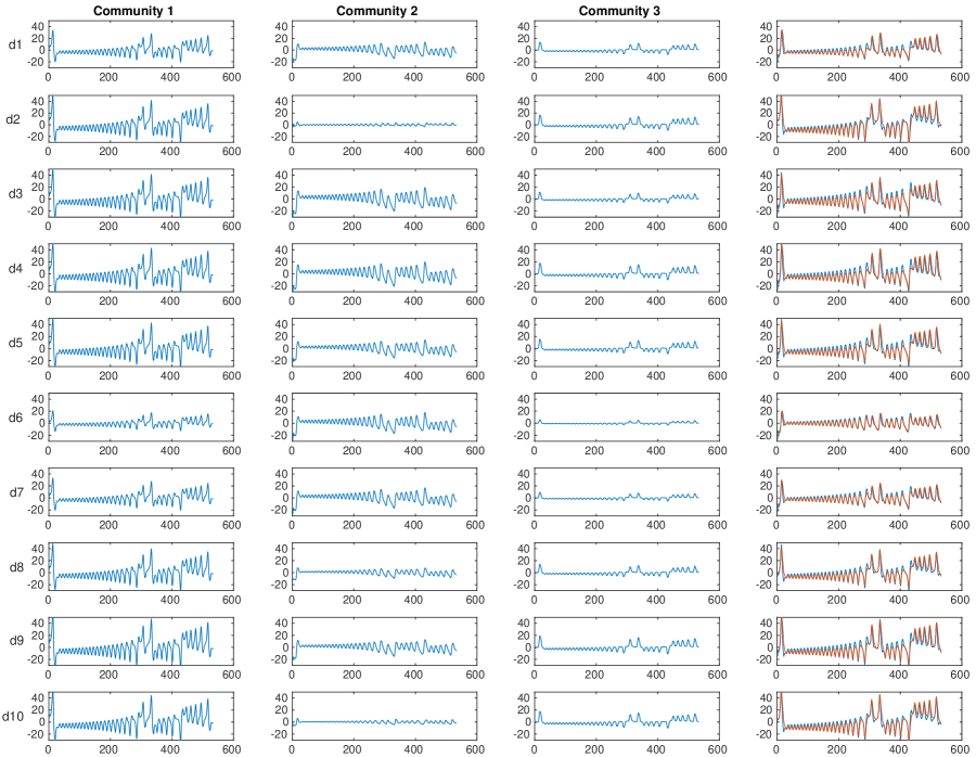
Figure 2: Visualization of community specific sub-sequences decomposed from the Lorenz Attractor based time series reconstructed by GGP-LDS. The first three columns show the sub-sequences of the three strongest communities, with each row showing one of the 10 data dimensions. The last column shows the superposition of the three sub-sequences shown in the first three columns, where the observed time series is also included for comparison (highlighted in red).

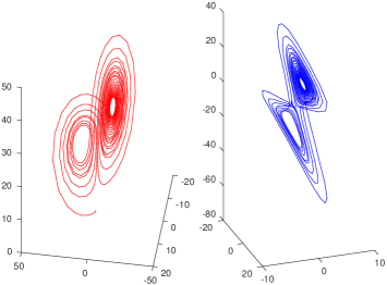
(a)

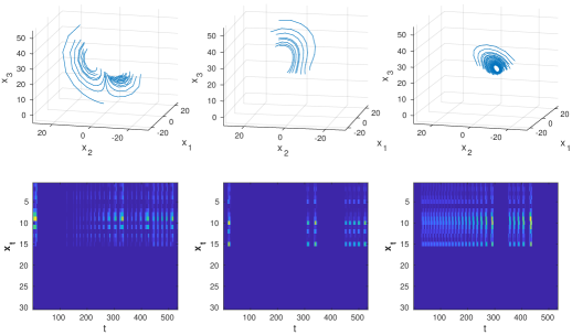
(b)

Figure 3: (a): The red trajectory shown on the left is synthesized by a Lorenz Attractor and used as the 3D latent state sequence to generate $\bm{y}_{1:T}$, a 10D time series observation. Training GGP-LDS on $\bm{y}_{1:T}$, the blue trajectory shown on the right is a 3D visualization of the inferred latent dynamics based on $(\hat{\bm{x}}_{1:T}^{(1)},\hat{\bm{x}}_{1:T}^{(2)},\hat{\bm{x}}_{1:T}^{(3)})$, the sub-sequences of the three strongest communities decomposed from the reconstructed time series by GGP-LDS.
   (b): The bottom row visualizes the inferred latent states $\bm{x}_{1:T}$ of GGP-LDS, which are assigned into three non-overlapping clusters via the $K$-means algorithm, and the top row visualizes the corresponding segments of the Lorenz Attractor synthesized 3D time series.

Out of $K=16$ (truncation level) possible communities, we show in Fig. 6(a) the top six formed communities, extracted from the inferred transition matrix for Lorenz Attractor, in six different subplots; we display each of these six communities using its relative strength defined in (6). It is shown in Fig. 1(b) that our nonparametric Bayesian model finds four communities in total to model the underlying pattern of the data. The number of linear solutions that our model has discovered is similar to that of Nassar et al. (2018), in which a tree based stick breaking process has been used as the prior. Moreover, it can be observed from Figs. 1(a) and 1(b) that these 4 active communities are formed over 15 active states. Note for GGP-LDS, we have truncated its number of communities at $K=16$ and that of states at $S=30$. The results in Fig. 1 have demonstrated the ability of GGP-LDS in inferring a parsimonious set of active communities and states to model the time series.

Fig. 2 shows how each community can reconstruct the observed data. Each row corresponds to a data dimension of the observed time series. The first three columns show how the three strongest communities contribute to data reconstruction, while the last column shows the superpositions of the first three columns and compares them against the observed time series. It can be seen from Fig. 2 that the different dimensions of each community specific sub-sequence share similar temporal patterns, but may exhibit clearly different magnitudes.

In Fig. 3(a), the red trajectory in the left plot represents the Lorenz Attractor synthesized 3D time series that is used as the latent state representation to generate the observed 10D time series, and the blue trajectory in the right plot illustrates a 3D representation of the latent dynamics of GGP-LDS trained on this 10D time series. More specifically, the blue trajectory is the visualization of the inferred community-specific latent sub-sequences ($\hat{\bm{x}}_{1:T}^{(1)},\hat{\bm{x}}_{1:T}^{(2)},\hat{\bm{x}}_{1:T}^{(3)}$), where $\hat{\bm{x}}_{1:T}^{(\kappa)}$, defined as in (7), is the latent sub-sequence extracted according to the relative strength of the $\kappa^{th}$ strongest community to the aggregation of all communities, as illustrated in Figs. 1(b) and 2 and described in detail in Algorithm 1. It can be seen from Fig. 3(a) that the latent dynamics ($e.g.$, moving between two spirals) of GGP-LDS, visualized in 3D based on its inferred sub-sequences of its three strongest communities, are closely synchronized with the underlying dynamics of the Lorenz Attract synthesized 3D time series (a video showing how the red and blue trajectories move synchronously with each other has been included). This shows that our model infers a close linear approximation to the underlying nonlinear dynamics.

We provide another visualization of the latent dynamics inferred by GGP-LDS in Fig. 3(b). Instead of decomposing the time series into sub-sequences, we now cluster it in time according to the inferred latent states $\bm{x}_{t}$. In the bottom row of Fig. 3(b), the $\bm{x}_{t}$’s are partitioned into three non-overlapping clusters with the $K$-means algorithm, which means each $\bm{x}_{t}$ is assigned to one of the three clusters. In the top row of Fig. 3(b), the same cluster assignment is applied to segment the Lorenz Attractor time series into three sequences that do not overlap in time. It is clear that the segmentation points based on the $\bm{x}_{t}$’s inferred by GGP-LDS well align with the switching points between different linear dynamics, demonstrating the ability of GGP-LDS to seamlessly transit between different temporal patterns, each of which is modeled by adjusting the activation strengths of different latent state communities that can co-occur at the same time.

Table 1: Lorenz Attractor predictive performance. The best result and the results that are not considered as statistically different are highlighted in bold.

Mean absolute error for 10 forecast horizons
Algorithm	$t=1$	$t=2$	$t=3$	$t=4$	$t=5$	$t=6$	$t=7$	$t=8$	$t=9$	$t=10$
LDS	$11.12_{(1.10)}$	$13.76_{(2.47)}$	$18.54_{(2.78)}$	$22.34_{(2.90)}$	$18.81_{(3.18)}$	$13.12_{(3.30)}$	$9.68_{(2.87)}$	$8.54_{(2.37)}$	$7.21_{(2.51)}$	$7.54_{(2.48)}$
rLDSg	$8.12_{(0.90)}$	$12.76_{(1.31)}$	$17.33_{(1.98)}$	$20.52_{(1.61)}$	$15.62_{(2.05)}$	$10.54_{(3.21)}$	$8.62_{(3.28)}$	$9.42_{(3.65)}$	$7.46_{(3.16)}$	$6.28_{(3.49)}$
rLDSr	$12.46_{(1.72)}$	$19.22_{(3.72)}$	$21.51_{(4.22)}$	$25.32_{(3.67)}$	$18.21_{(3.11)}$	$11.51_{(4.16)}$	$13.21_{(4.21)}$	$10.21_{(4.11)}$	$8.57_{(3.95)}$	$6.91_{(3.18)}$
SGLDS	$8.84_{(1.32)}$	$10.43_{(1.66)}$	$14.51_{(2.43)}$	$15.32_{(3.61)}$	$16.31_{(3.24)}$	$15.32_{(3.83)}$	$12.21_{(3.94)}$	$9.13_{(4.24)}$	$9.57_{(3.95)}$	$7.91_{(3.68)}$
TrSLDS	$5.21_{(0.62)}$	$5.76_{(0.98)}$	$6.23_{(1.31)}$	$7.45_{(1.42)}$	$\mathbf{5.31_{(1.19)}}$	$\mathbf{5.12_{(1.53)}}$	$\mathbf{4.21_{(1.24)}}$	$\mathbf{2.31_{(1.18)}}$	$\mathbf{2.57_{(1.45)}}$	$\mathbf{5.78_{(1.11)}}$
Multi-output GP	$11.52_{(1.58)}$	$15.35_{(1.73)}$	$16.21_{(2.21)}$	$19.08_{(2.36)}$	$17.21_{(3.79)}$	$12.37_{(3.77)}$	$8.38_{(3.98)}$	$8.21_{(2.98)}$	$6.31_{(3.21)}$	$7.21_{(3.98)}$
FB Prophet	$5.57_{(1.31)}$	$11.82_{(1.45)}$	$13.42_{(1.98)}$	$15.21_{(2.04)}$	$16.26_{(1.76)}$	$9.41_{(1.86)}$	$8.78_{(2.01)}$	$7.66_{(1.91)}$	$6.54_{(2.14)}$	$6.72_{(2.23)}$
DeepAR	$9.42_{(0.26)}$	$10.21_{(0.31)}$	$16.22_{(0.54)}$	$16.42_{(1.28)}$	$15.24_{(1.21)}$	$11.21_{(1.61)}$	$13.25_{(2.08)}$	$12.83_{(2.83)}$	$14.21_{(3.01)}$	$16.25_{(3.21)}$
TRCRP	$5.66_{(0.86)}$	$7.91_{(1.01)}$	$11.23_{(1.35)}$	$15.37_{(2.31)}$	$16.21_{(2.42)}$	$9.68_{(2.68)}$	$8.21_{(2.98)}$	$6.85_{(2.71)}$	$5.63_{(2.38)}$	$7.35_{(2.81)}$
GGP-LDS (10 steps)	$\mathbf{2.12_{(0.84)}}$	$\mathbf{3.76_{(1.87)}}$	$\mathbf{4.77_{(2.68)}}$	$\mathbf{5.04_{(3.16)}}$	$\mathbf{4.83_{(3.32)}}$	$\mathbf{4.50_{(3.27)}}$	$\mathbf{4.15_{(3.34)}}$	${4.14_{(3.51)}}$	${4.60_{(3.66)}}$	$\mathbf{5.24_{(3.86)}}$
GGP-LDS (1 step)	$2.10_{(0.52)}$	$0.37_{(0.23)}$	$0.32_{(0.17)}$	$0.41_{(0.18)}$	$0.40_{(0.24)}$	$0.64_{(0.27)}$	$0.84_{(0.28)}$	$0.81_{(0.25)}$	$0.66_{(0.23)}$	$0.57_{(0.23)}$

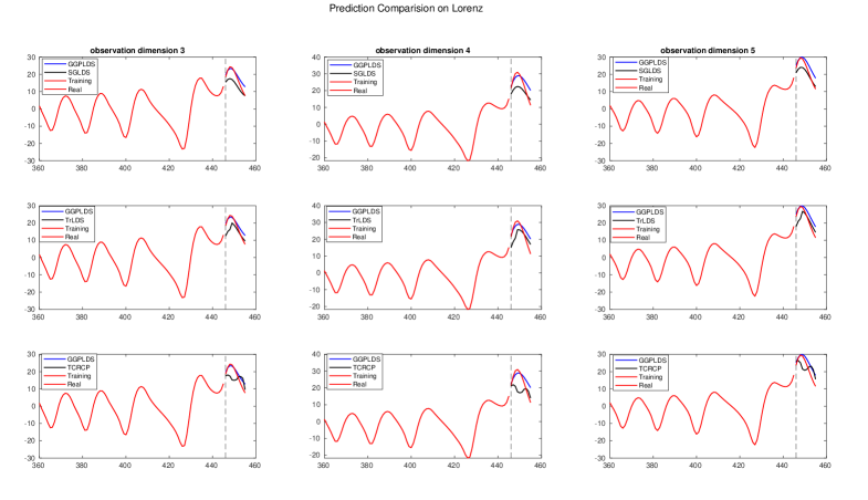
Figure 4: Comparison of predictive performance of the GGPLDS to SGLDS, TrSLDS and TRCRP on Lorenz attractor data. Each column of the figure represents one dimension of the observation (out of 10) and each row contain the visual comparison of GGP-LDS with one of those aforementioned algorithms.

In addition to these qualitative analyses, we quantitatively compare GGP-LDS and a variety of baseline algorithms on their predictive performance on the same 10D time series $\bm{y}_{t}$, generated by adding Gaussian noise to ${\bf D}\bm{x}_{t}$, where $\bm{x}_{1:T}$ is a Lorenz Attractor synthesized 3D time series. Below we list the parameter settings of the baseline algorithms; for each competing algorithm, we choose its setting on each dataset that provides it the best overall prediction performance over 10 forecast horizons, except for SGLDS and GGP-LDS that are insensitive to hyperparameter settings under their respective nonparametric Bayesian constructions:

• LDS of Ghahramani and Hinton (1996), inferred by EM, with $K=6$.

• $rLDS_{g}$ and $rLDS_{r}$ of Liu and Hauskrecht (2015), with $K=8$ and random initialization.

• SGLDS of Kalantari et al. (2018), with the number of hidden states truncated at $K=30$.

• TrSLDS of Nassar et al. (2018), with its tree depth set as 2 and dimension of latent states for each LDS as 4.

• Multi-outputGP of Alvarez and Lawrence (2009), setting: 1. multi-gp option, 2. kerneltype: ggwhite, 3. optimizer: scg, 4. nlf = 1.

• FB Prophet of Taylor and Letham (2018), default setting.

• Deep AR of Flunkert et al. (2017), default setting.

• TRCRP of Saad and Mansinghka (2018), with the Markov chain order set as $p=10$ .

As $t=445$ is one of the switching time points at which $\bm{x}_{t}$ moves from one spiral to another, we choose $\bm{y}_{1:445}$ for training. This set up can measure how well an algorithm detects and responds to changes in the underlying dynamics. The predictive performance of each algorithm is measured by mean absolute error defined in 10 over a horizon of 10 time points. The results are presented in Table 1. As shown in Table 1, most of the competing algorithms are not making good predictions following the switching point, likely because they expect that the trajectory will keep following the same spiral pattern before the switching point. In reality, the trajectory quickly switches to the other spiral pattern for a few steps before coming back to the same spiral pattern observed before $t=445$. To further illustrate this point, we pick three different dimensions of the 10D time series $\bm{y}_{t}$, and show in Fig. 4 the prediction of four different algorithms, including SGLDS, TrLDS, TCRCP, and the proposed GGP-LDS, on these three dimensions over a horizon of 10 time points. It is evident from Fig. 4 that at the switching point, SGLDS, TrLDS, and TCRCP all fail to detect the transition from one spiral to another. More specifically, SGLDS closely follows the pattern of the same spiral, TrSLDS is experiencing delays in switching to the correct LDS that better fits the second spiral, and TRCRP creates wrong patterns.

4.2 FitzHugh-Nagumo

We provide another set of visualization of GGP-LDS by considering the FitzHugh-Nagumo (FHN) model, which can be formulated by the following differential equations:

$$\frac{dv}{dt}=v-\frac{v^{3}}{3}-w+I,$$

$$\frac{dw}{dt}=c\times\left(v+a-bw\right).$$

We set $I=0.3$, $a=0.7$, $b=0.8$, and $c=0.7$. We train our model with a trajectory whose starting point is picked randomly. The trajectory consists of 800 time points. The observation model is linear and Gaussian where $\bm{d}_{i}\sim\mathcal{N}\left([0,0]^{T},\left(\begin{matrix}1&0\\ 0&1\end{matrix}\right)\right)$ and $\bm{\Phi}=0.01*\mathbf{I}_{2}$, where $\mathbf{I}_{2}$ is an identity matrix of dimension $2\times 2$. We provide a set of plots analogous to those in Figs 1(a), 1(b), and 3(a) for Lorenz Attractor. It can be seen in Fig. 5 how the latent trajectories have been recovered by ($\hat{\bm{x}}_{c_{1}},\hat{\bm{x}}_{c_{2}}$) that represent the activation strength of the two strongest communities $(c_{1},c_{2})$.

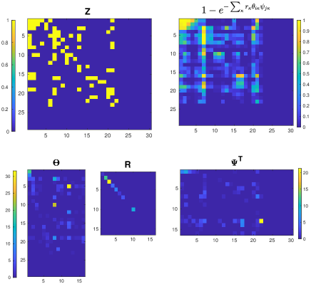
(a)

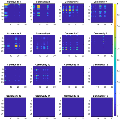
(b)

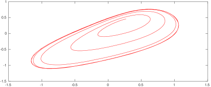
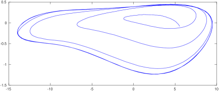
(c)

Figure 5: Visualization of a posterior sample of GGP-LDS applied to FitzHugh-Nagumo, where (a), (b), and (c) are analogous plots to Figs. 1(a), 1(b), and 3(a), respectively.

4.3 Pedestrians’ Trajectories

We analyze a dataset that records by camera the 3D motions of pedestrians and their interactions, downloaded from https://motchallenge.net/ and available in the provided code repository. For visualization purpose, we use only 2 dimensional data for each pedestrian $(x,y)$. We select six pedestrians over 120 time points to train our model. The next 10 time points are used to measure the predictive performance of various algorithms.

Table 2 compares the predictive performance of various algorithms on this dataset. In most of the 10 forecast horizons our model has outperformed the other competing models. The parameter settings of various algorithms are the same as those in Section 4.1 for Lorenz Attractor, with the following exceptions:

• LDS of Ghahramani and Hinton (1996), inferred by EM, with $K=8$.

• TrSLDS of Nassar et al. (2018), with its tree depth set as 2 and dimension of latent states for each LDS as 2.

Table 2: Analogous table to Table 1 for the Pedestrians dataset

Mean absolute error for 10 forecast horizons
Algorithm	$t=1$	$t=2$	$t=3$	$t=4$	$t=5$	$t=6$	$t=7$	$t=8$	$t=9$	$t=10$
LDS	$0.21_{(0.09)}$	$0.31_{(0.17)}$	$1.10_{(0.41)}$	$1.27_{(0.46)}$	$1.55_{(0.66)}$	$1.48_{(0.65)}$	$1.52_{(0.62)}$	$1.62_{(0.61)}$	$1.60_{(0.59)}$	$1.76_{(0.71)}$
rLDSg	$0.19_{(0.07)}$	$0.29_{(0.12)}$	$0.41_{(0.19)}$	$0.71_{(0.16)}$	$1.11_{(0.23)}$	$1.08_{(0.59)}$	$1.12_{(0.65)}$	$1.27_{(0.58)}$	$1.37_{(0.61)}$	$1.41_{(0.70)}$
SGLDS	$0.17_{(0.12)}$	$0.24_{(0.16)}$	$0.28_{(0.23)}$	$0.42_{(0.21)}$	$0.54_{(0.34)}$	$0.66_{(0.31)}$	$0.71_{(0.41)}$	$0.87_{(0.44)}$	$0.97_{(0.55)}$	$1.02_{(0.68)}$
TrSLDS	$0.16_{(0.10)}$	$0.26_{(0.12)}$	$0.32_{(0.18)}$	$0.40_{(0.21)}$	$0.52_{(0.28)}$	$0.60_{(0.29)}$	$0.69_{(0.32)}$	$0.79_{(0.39)}$	$0.79_{(0.41)}$	$0.92_{(0.48)}$
Multi-output GP	$0.22_{(0.11)}$	$0.28_{(0.16)}$	$0.42_{(0.21)}$	$0.60_{(0.20)}$	$0.68_{(0.21)}$	$0.89_{(0.17)}$	$1.03_{(0.23)}$	$1.15_{(0.28)}$	$1.41_{(0.32)}$	$1.40_{(0.30)}$
FB Prophet	$0.17_{(0.05)}$	$0.26_{(0.08)}$	$0.33_{(0.11)}$	$0.40_{(0.12)}$	$0.56_{(0.14)}$	$0.65_{(0.14)}$	$0.87_{(0.13)}$	$0.86_{(0.17)}$	$1.04_{(0.23)}$	$1.12_{(0.20)}$
DeepAR	$0.22_{(0.06)}$	$0.21_{(0.04)}$	$0.32_{(0.04)}$	$0.42_{(0.12)}$	$0.64_{(0.21)}$	$0.81_{(0.27)}$	$0.85_{(0.31)}$	$0.98_{(0.36)}$	$1.03_{(0.45)}$	$1.15_{(0.51)}$
TRCRP	$0.17_{(0.09)}$	$0.19_{(0.10)}$	$0.29_{(0.12)}$	$\mathbf{0.27_{(0.16)}}$	$\mathbf{0.33_{(0.21)}}$	$\mathbf{0.38_{(0.15)}}$	$0.61_{(0.22)}$	$0.66_{(0.28)}$	$0.71_{(0.32)}$	$0.92_{(0.38)}$
GGP-LDS (10 steps)	$\mathbf{0.14_{(0.11)}}$	$\mathbf{0.20_{(0.16)}}$	$\mathbf{0.26_{(0.21)}}$	$0.31_{(0.26)}$	$0.38_{(0.32)}$	$0.44_{(0.37)}$	$\mathbf{0.52_{(0.44)}}$	$\mathbf{0.59_{(0.50)}}$	$\mathbf{0.67_{(0.57)}}$	$\mathbf{0.75_{(0.64)}}$
GGP-LDS (1 step)	$0.11_{(0.08)}$	$0.13_{(0.09)}$	$0.14_{(0.11)}$	$0.14_{(0.11)}$	$0.15_{(0.12)}$	$0.17_{(0.13)}$	$0.19_{(0.14)}$	$0.21_{(0.16)}$	$0.23_{(0.18)}$	$0.26_{(0.21)}$

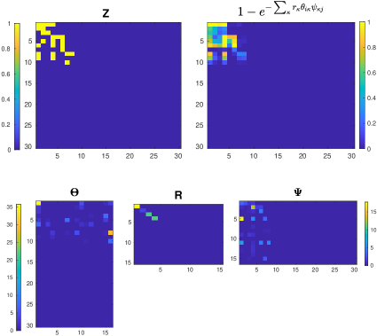
(a)

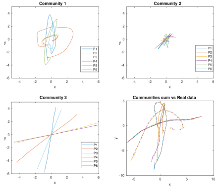
(b)

Figure 6: Visualization of a posterior sample of GGP-LDS applied to the Pedestrian dataset, where (a) and (b) are analogous plots to Figs. 1(a) and 2, respectively.

Fig. 6(a) provides the interpretation of the latent factors for this dataset, analogous to Fig. 1(a) used to provide interpretation of the latent structure inferred from Lorenz Attractor. Fig. 6(b), analogous to Fig. 2 for Lorenz Attractor, represents the reconstruction of all 6 pedestrians’ trajectories using the three strongest communities. A total of four communities is inferred by GGP-LDS to model the underlying pattern of the data. Fig. 6(b) shows how each community can decompose the observed data in 2 dimensions $(x,y)$ into a community-specific sub-sequence. The last subplot superposes the first three sub-sequences and compares it against the true trajectory (shown in dashed lines).

It is interesting to see how each community can create one type of motion ($e.g.$, straight movement, circular trajectory, and spiral movement). It is evident that regardless of the property of motion, such as “turn direction,” “radius of circular motion,” or “direction of straight,” the trajectories of the same nature have appeared in a same community-specific sub-sequence. It can be seen in the figure that some of the communities have a very small contribution for some of the pedestrians’ trajectory reconstruction since those pedestrians did not use that specific pattern in their recorded walking.

4.4 Stock Price

Table 3: Analogous table to Table 1 for the Stock Price dataset

Mean absolute error for 10 forecast horizons
Algorithm	$t=1$	$t=2$	$t=3$	$t=4$	$t=5$	$t=6$	$t=7$	$t=8$	$t=9$	$t=10$
LDS	$0.07_{(0.01)}$	$0.06_{(0.02)}$	$0.07_{(0.01)}$	$0.07_{(0.02)}$	$0.08_{(0.02)}$	$0.08_{(0.02)}$	$0.09_{(0.02)}$	$0.08_{(0.02)}$	$0.09_{(0.03)}$	$0.10_{(0.02)}$
rLDSg	$0.03_{(0.07)}$	$0.03_{(0.01)}$	$0.04_{(0.19)}$	$0.04_{(0.01)}$	$0.06_{(0.01)}$	$0.06_{(0.02)}$	$0.06_{(0.02)}$	$0.07_{(0.02)}$	$0.08_{(0.02)}$	$0.09_{(0.02)}$
SGLDS	$0.05_{(0.01)}$	$0.05_{(0.01)}$	$0.06_{(0.02)}$	$0.06_{(0.02)}$	$0.06_{(0.03)}$	$0.08_{(0.02)}$	$0.08_{(0.03)}$	$0.09_{(0.03)}$	$0.09_{(0.03)}$	$0.10_{(0.04)}$
TrSLDS	$0.03_{(0.01)}$	$0.04_{(0.01)}$	$0.04_{(0.02)}$	$\mathbf{0.05_{(0.02)}}$	$0.06_{(0.03)}$	$0.07_{(0.02)}$	$0.07_{(0.03)}$	$0.08_{(0.03)}$	$0.08_{(0.03)}$	$0.09_{(0.03)}$
Multi-output GP	$0.09_{(0.03)}$	$0.08_{(0.03)}$	$0.10_{(0.03)}$	$0.13_{(0.03)}$	$0.11_{(0.03)}$	$0.10_{(0.02)}$	$0.12_{(0.03)}$	$0.12_{(0.03)}$	$0.13_{(0.03)}$	$0.14_{(0.03)}$
FB Prophet	$\mathbf{0.01_{(0.02)}}$	$\mathbf{0.03_{(0.01)}}$	$0.06_{(0.01)}$	$0.08_{(0.02)}$	$0.07_{(0.01)}$	$0.08_{(0.02)}$	$0.09_{(0.02)}$	$0.08_{(0.02)}$	$0.09_{(0.03)}$	$0.10_{(0.02)}$
DeepAR	$0.05_{(0.01)}$	$0.05_{(0.02)}$	$0.06_{(0.02)}$	$0.06_{(0.03)}$	$0.07_{(0.02)}$	$0.08_{(0.03)}$	$0.08_{(0.03)}$	$0.09_{(0.03)}$	$0.09_{(0.04)}$	$0.10_{(0.03)}$
TRCRP	$0.03_{(0.01)}$	$0.04_{(0.02)}$	$0.04_{(0.01)}$	${0.06_{(0.01)}}$	${0.07_{(0.02)}}$	$\mathbf{0.05_{(0.02)}}$	$\mathbf{0.04_{(0.02)}}$	$\mathbf{0.03_{(0.01)}}$	$\mathbf{0.05_{(0.01)}}$	$0.07_{(0.02)}$
GGP-LDS (10 steps)	$0.03_{(0.01)}$	$\mathbf{0.03_{(0.01)}}$	$\mathbf{0.03_{(0.01)}}$	$0.05_{(0.02)}$	$\mathbf{0.05_{(0.01)}}$	$\mathbf{0.05_{(0.01)}}$	$0.05_{(0.01)}$	$0.05_{(0.02)}$	$0.06_{(0.02)}$	$\mathbf{0.07_{(0.02)}}$
GGP-LDS (1 step)	$0.02_{(0.01)}$	$0.02_{(0.01)}$	$0.02_{(0.01)}$	$0.03_{(0.01)}$	$0.02_{(0.01)}$	$0.02_{(0.01)}$	$0.02_{(0.01)}$	$0.02_{(0.01)}$	$0.04_{(0.01)}$	$0.05_{(0.02)}$

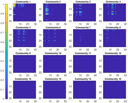
(a)

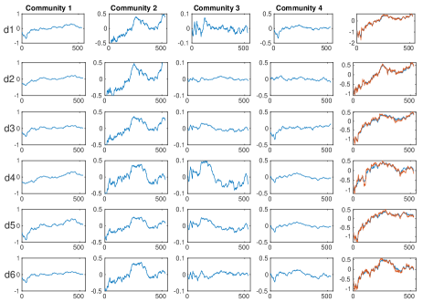
(b)

Figure 7: Visualization of GGP-LDS applied to stock closing prices. (a) Inferred communities, analogous plot to Fig. 1(b) (b) Inferred community-specific sub-sequences of the four strongest communities and their superpositions, analogous plot to Fig. 2.

This dataset contains 12 companies’ relative closing price ($P_{t}-P_{t-1}$) over the course of three years. These 12 companies have been selected from four different industries, and the stock closing prices of the ones in the same industry share similar temporal behaviors. Table 4 compares the predictive performance of various algorithms on this dataset. In most of the 10 forecast horizons our model has outperformed the other competing models. The parameter settings of various algorithms are the same as those in Section 4.1 for Lorenz Attractor, with the following exceptions:

• LDS of Ghahramani and Hinton (1996), inferred by EM, with $K=12$.

• $rLDS_{g}$ of Liu and Hauskrecht (2015), with $K=14$ and random initialization.

• TrSLDS of Nassar et al. (2018), with its tree depth set as 1 and dimension of latent states for each LDS as 8.

Fig. 7(a) shows the formed communities. Eight non-zero communities has been formed with the first four communities having at least one non-overlapping member, while the next four communities do not have members that are exclusive to them. Having four major communities, Fig. 7(b) shows how each of these major communities can contribute to reconstruct the observed data. Rows of Fig. 7(b) correspond to 6 stocks out of 12. The first four columns of the figure describe how the four strongest detected communities contributed to reconstruct the data in each dimension. There are two noticeable observations in Fig. 7(b). First, it can be seen that each community represents similar behavior for all 6 selected stocks in the figure, and these behaviors are distinct from one community to another. Second, it is evident that if a behavior represented by a community does not play a significant role in reconstruction of the data in a specific dimension, that community contribution will be trivial. As an example, community 3’s role in reconstructing the second stock is trivial, while playing a much more significant role to reconstruct the observation of the fourth stock.

4.5 Daily new COVID-19 Cases

This dataset contains the daily reported COVID-19 cases in each of the 50 States and District of Columbia from the beginning of March to end of May 2020. For predictive performance comparison, we have compared our model against two models which have been specifically developed to understand the COVID-19 pandemic: Zou et al. (2020) use a differential equation based epidemic model and use differential equation solver to find the model parameters; Woody et al. (2020) utilize the social distancing data as covariates and a statistical model negative binomial regression model utilizing these covariates to predict the intensity of pandemic in the future. Table 4 shows the $6$-steps predictive performance of GGP-GLDS on this dataset. For the competing algorithms in Table 4, we list the parameter settings below:

• TrSLDS of Nassar et al. (2018), with its tree depth set as 1 and dimension of latent states for each LDS as 5.

• TRCRP of Saad and Mansinghka (2018), with the Markov chain order set as $p=6$ .

• UCLA-SuEIR of Zou et al. (2020)

• UT-Mobility of Woody et al. (2020)

Table 4: Prediction of daily new Covid-19 cases in the U.S. given daily observations from March 6 to May 23, 2020.

Mean absolute relative error for 6 forecast horizons
Algorithm	$t=1$	$t=2$	$t=3$	$t=4$	$t=5$	$t=6$
Year 2020	May 24	May 25	May 26	May 27	May 28	May 29
TrSLDS	$6.68_{(2.31)}$	$7.21_{(3.28)}$	$6.18_{(3.08)}$	${5.25_{(2.42)}}$	$1.87_{(2.8)}$	$8.85_{(3.27)}$
UCLA Covid19	$\mathbf{3.87_{(1.68)}}$	${4.86_{(1.51)}}$	$5.23_{(2.25)}$	$3.23_{(2.27)}$	$2.87_{(1.96)}$	$6.61_{(4.18)}$
UT-Austin Covid19	$6.32_{(2.51)}$	$5.38_{(2.73)}$	$6.26_{(3.25)}$	$3.78_{(2.13)}$	$3.16_{(2.02)}$	$7.95_{(3.93)}$
TRCRP	$7.66_{(3.81)}$	$6.27_{(3.25)}$	$7.22_{(3.36)}$	${4.21_{(2.86)}}$	${2.31_{(1.37)}}$	$\mathbf{6.11_{(3.25)}}$
GGP-GLDS (6 steps)	$4.78_{(2.95)}$	$\mathbf{4.47_{(2.27)}}$	$\mathbf{3.71_{(1.12)}}$	$\mathbf{1.68_{(5.67)}}$	$\mathbf{0.69_{(0.42)}}$	${9.50_{(18.01)}}$

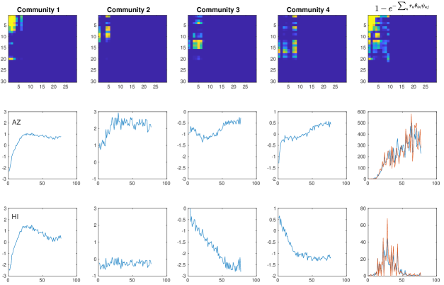
Figure 8: Visualization of GGP-GLDS (NBDS) applied to U.S. COVID-19 daily cases. Row 1 shows the relative activation strengths of the four strongest communities, analogous to Fig. 1(b); Rows 2 and 3 show the inferred community-specific sub-sequences of the four strongest communities and the expected counts given their superpositions.

Similar to previous visualizations, the first row of Fig. 8 shows the relative strengths of four discovered communities that have at least one non-overlapping member, with the last column of the first row representing $1-e^{-\sum_{\kappa}r_{\kappa}\theta_{i\kappa}\psi_{j\kappa}}$. The relative strength of a community is defined as in (6). The second row shows the trajectories for Arizona (AZ), with the trajectory in each of its first four columns showing a community-specific sub-sequence for AZ, which is the corresponding row of ${\bf D}\hat{\bm{x}}_{1:T}^{(\kappa)}$, where $\hat{\bm{x}}_{t}^{(\kappa)}=[({{\bf W}}\odot{\bf Z})\odot{{\bf A}}_{\kappa}]\bm{x}_{t-1}$ is defined as in (7); the last column of the second row compares the trajectory obtained by

$$\hat{\bm{y}}_{t}^{(\kappa)}:=\eta e^{(\sum_{\kappa=1}^{4}{\bf D}\hat{\bm{x}}_{t}^{(\kappa)})}$$

against the true trajectory of AZ, which shows how discovered communities can reconstruct the observed time series at different data dimensions. Shown in the third row are analogous plots for Hawaii (HI).

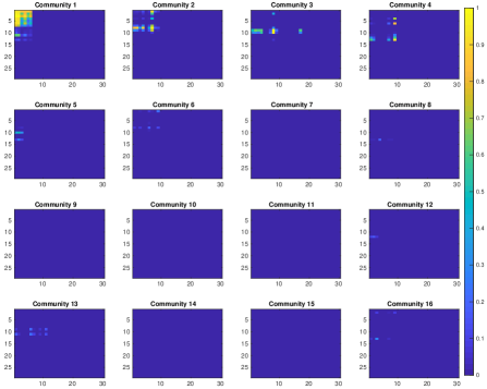
(a)

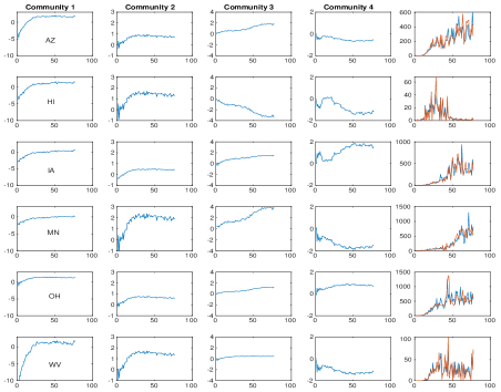
(b)

Figure 9: Visualization of a posterior sample (different from the sample used for Fig. 8) of GGP-GLDS (NBDS) applied to U.S. daily new COVID-19 cases. (a): Inferred communities, analogous to Fig. 1(b); (b): Inferred community-specific sub-sequences of the four strongest communities and their superpositions, analogous to Fig. 2.

Fig. 9(a) shows all discovered communities, out of which the first four communities have at least one non-overlapping member unique to themselves. Please note that the discovered communities and adjacency matrix of the posterior sample in Fig. 9 are different from those in Fig. 8. We intentionally choose two different samples from 2 different runs with different random seeds to show the consistency of interpretation across different runs. Although these two posterior samples come from two independent Markov chains initialized with different random seeds, and consequently different adjacency matrices, the algorithm still finds 4 communities with at least one non-overlapping member, and Figs. 9(b) and 8 show that the interpretation of the communities stay consistent from one run to another. This consistency of interpretation helps to show that no specific method for model parameter initialization is required for the proposed GGP-GLDS.

Similar to previous visualizations, there are two noticeable observations from Figs. 8 and 9(b). First, it can be seen how each community represents a distinct behavior shared by all data dimensions at different magnitudes. Second, a behavior represented by a community may play a negligible role in reconstructing the data in a specific dimension if its corresponding magnitude is small.

5 Discussion and Conclusion

We introduce the graph gamma process (GGP) to form an infinite dimensional transition model with a finite random number of nonzero-degree nodes and a finite random number of nonzero-edge communities over these nodes. The GGP is used to promote sparsity on the state-transition matrix of a (generalized) linear dynamical system, and encourage forming overlapping communities among the nonzero-degree nodes of the graph. The model is designed such that each node community models a behavior described with a linear dynamical system. Instead of assigning one behavior to a temporal segment of an observation trajectory, it allows the whole time series to be viewed as a superposition of distinctly behaved trajectories, each of which is modeled by one of the discovered overlapping communities. These overlapping communities can be activated at different levels at different time points to support the superposition to have sophisticated temporal behavior, allowing smooth transitions between different linear dynamics to approximate nonlinear dynamical behaviors.

This paper focuses on time-series data modeling using a nonparametric Bayesian hierarchical model. The main challenges for modeling the time series include accurate forecast, missing data imputation, and meaningful clustering of the latent variables of the model such that these clusters can be translated to meaningful underlying patterns of the data, which represent different behaviors in a dataset without requiring data specific customization. The main goal of this paper is to develop a nonparametric Bayesian model to find a flexible solution that provides interpretable latent representation and have good predictive performance. The nonparametric Bayesian construction of the model introduced in this paper prevents the underlying model from being over- and under-parameterized, which can result in over- or under-fitting, respectively, and hence poor performance in forecasting. In addition, the model learns a parsimonious graph among the infinite dimensional latent variables such that the induced clusters by community forming among non-zero-degree states can explain the underlying patterns of the data without the need of manual tuning. The nonparametric Bayesian construction and shrinkage property of the GGP introduced in this paper avoid inducing too many latent communities over too many latent states that will make the model difficult to interpret. Our experiments show that GGP-(G)LDS creates good balance between interpretability and predictive performance. Using the formed overlapping communities over the inferred set of latent states, the model is capable of modeling non-linearity in the data by creating multiple linear systems which try to learn the underlying non-linear behavior of the data. The model can break the sophisticated behavior in a trajectory to the combination of simpler behaviors modeled by linear dynamical systems, and it helps to model the nonlinearity of the data using multiple linear dynamical systems and smooth transition between them. The linear approximation of data with nonlinear dynamics enables the proposed GGP-LDS to leverage existing smoothing and filtering algorithms readily available to canonical LDSs.

Furthermore, this model can be seen as a generalization to existing nonparametric Bayesian linear dynamical systems from two different perspectives. First, the formed communities with overlapping members will translate to the soft switching concept among latent communities (or different LDSs) such that the strength of each LDS at any given time can change using the overlapping states which have replaced the hard switching among the different LDSs in switching LDSs. The hard switch is prone to picking a false LDS at the switching point, and results in wrong interpretation and deteriorated predictive performance. Second, unlike switching LDSs, the proposed model does not make any assumption on the dimensions of latent states, which are often set to be different in switching LDSs for different segments of the trajectory.

In addition, we show by an example how the proposed model with minor change in observation layer can turn to a model for generalized linear models (GLM) which helps us to model overdispersed count data, which often seriously violates the Gaussian assumption on observations. That adaptability helps us to model the trajectories of daily new COVID-19 cases in each State of the US by training the model on multivariate count observations across the 50 States and D.C., and hope its interpretability and predictive performance could help decision makers in pattern discovery, resource assignment, and predictive analytics related tasks. An on-going effort is using the proposed negative binomial dynamical system to jointly model the number of daily COVID-19 cases and deaths across all the States at the U.S. and provide forecast for future COVID-19 cases and deaths.

Appendix A Graphical Model

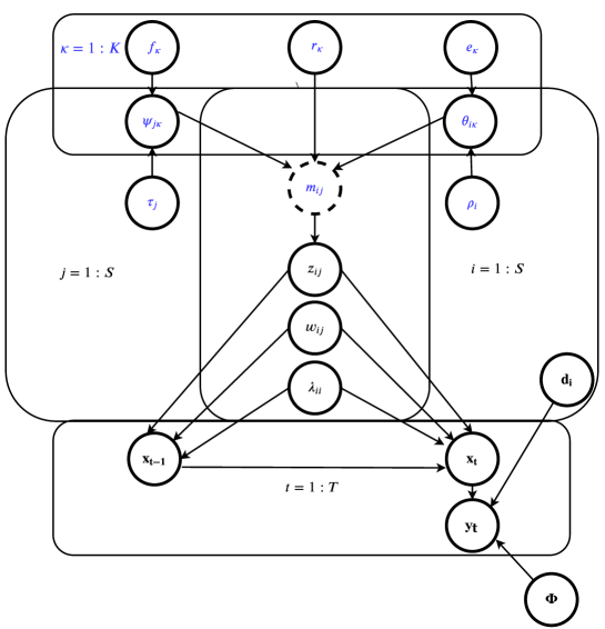
Figure 10: Graphical description of GGP-LDS.

Appendix B Proofs

Proof of Lemma 1.

We first notice $z_{ij\kappa}$ can be equivalently generated under the Bernoulli-Poisson link (Zhou, 2015) as

$$z_{ij\kappa}=\delta(m_{ijk}\geq 1),~{}m_{ij\kappa}\sim\mbox{Pois}(r_{\kappa}\theta_{i\kappa}\psi_{j\kappa}).$$

As $\sum_{i}\sum_{j}z_{ij\kappa}\leq\sum_{i}\sum_{j}m_{ij\kappa}$, it is sufficient to prove $\mathbb{E}[\sum_{i}\sum_{j}m_{ij\kappa}]$ is finite, which is true as $\mathbb{E}[\sum_{i}\sum_{j}m_{ij\kappa}]=r_{\kappa}\mathbb{E}[\sum_{i}\theta_{i\kappa}]\mathbb{E}[\sum_{j}\psi_{j\kappa}]=r_{\kappa}\gamma_{\rho}\gamma_{\tau}/(ef)$. ∎

Proof of Lemma 2.

Following the proof of Lemma 1, with model properties, $\textstyle{\bf Z}=\delta({\bf M}\geq 1),~{}{\bf M}\sim\mbox{Pois}(\sum_{k=1}^{\infty}r_{\kappa}\bm{\theta}_{\kappa}\bm{\psi}_{\kappa}^{T})$, we have $\mathbb{E}[\sum_{i}\sum_{j}z_{ij}]\leq\mathbb{E}[\sum_{i}\sum_{j}\sum_{\kappa}\gamma_{\kappa}\theta_{i\kappa}\psi_{j\kappa}]=\mathbb{E}[\sum_{\kappa}r_{\kappa}\gamma_{\rho}\gamma_{\tau}/(ef)]=\gamma_{0}\gamma_{\rho}\gamma_{\tau}/(cef)$. ∎

Below we show the total energy captured by all non-dynamic states is small: Due to the normal-gamma construction, for state $i$ we have

$$P(x_{1i},\ldots,x_{Ti}\,|\,a,b) =\textstyle\int_{0}^{\infty}\left[\prod_{t=1}^{T}\mathcal{N}(x_{ti};0,\lambda_{i}^{-1})\right]\mbox{Gamma}(\lambda_{i};a,1/b)\,d\lambda_{i}$$

$$=\textstyle\frac{b^{a}\Gamma(a+\frac{T}{2})}{(2\pi)^{\frac{T}{2}}\Gamma(a)}\left(b+\frac{1}{2}\sum_{t=1}^{T}x^{2}_{ti}\right)^{-\left(a+\frac{T}{2}\right)}.$$

Similar to the analysis in Tipping (2001), if we let $a=b=0$, we obtain an improper prior as $p(\sum_{t=1}^{T}x_{ti}^{2})\propto(\sum_{t=1}^{T}x_{ti}^{2})^{-T/2}$, which is sharply peaked at $\sum_{t=1}^{T}x_{ti}^{2}=0$. Thus choosing small $a$ and $b$, the proposed model will penalize the total energy captured by node (state) $i$, expressed as $\sum_{t=1}^{T}x^{2}_{ti}$, if it is a zero-degree node.

Appendix C Bayesian Inference via Gibbs Sampling

1. Sample $\omega_{vt}$ for GGD-GLDS. Using data augmentation for negative binomial regression, as in Zhou et al. (2012) and Polson et al. (2013), we denote $\omega_{vt}$ as a random variable drawn from the Polya-Gamma (PG) distribution (Polson and Scott, 2011) as $\omega_{vt}\sim\mbox{PG}\left(y_{vt}+\eta,~{}0\right),$ under which we have $\mathbb{E}_{\omega_{vt}}\left[\exp(-\omega_{vt}(\xi_{vt})^{2}/2)\right]={\cosh^{-(y_{vt}+\eta)}(\xi_{vt}/2)}$. Since $\bm{y}_{t}\sim{\mbox{NB}}(\eta,\sigma({\bf D}\bm{x}_{t}))$, the likelihood of ${\bm{\xi}}_{t}:={\bf D}\bm{x}_{t}$ can be expressed as

   $$\mathcal{L}({\bm{\xi}}_{t}) \propto\prod_{v=1}^{V}\frac{{(e^{\xi_{vt}})}^{y_{vt}}}{{(1+e^{\xi_{vt}})}^{y_{vt}+\eta}}$$

   $$=\prod_{v=1}^{V}\frac{2^{-(y_{vt}+\eta)}\exp({\frac{y_{vt}-\eta}{2}\xi_{vt}})}{\cosh^{y_{vt}+\eta}(\xi_{vt}/2)}$$

   $$\propto\prod_{v=1}^{V}\exp\left({\frac{y_{vt}-\eta}{2}\xi_{vt}}\right)\mathbb{E}_{\omega_{vt}}\left[\exp[-\omega_{vt}(\xi_{vt})^{2}/2]\right].$$

   Combining the likelihood $\mathcal{L}(\xi_{vt},\omega_{vt})\propto\exp\left({\frac{y_{vt}-\eta}{2}\xi_{vt}}\right)\exp[-\omega_{vt}(\xi_{vt})^{2}/2]$ and the prior, we sample auxiliary PG random variables $\omega_{vt}$ as

   $$(\omega_{vt}\,|\,-)\sim\mbox{PG}\left(y_{vt}+\eta,~{}{\bf D}(v,:)\bm{x}_{t}\right),\vspace{0mm}$$ (12)

   where ${\bf D}(v,:)$ denotes the $v$th row of ${\bf D}$. Note to sample from the PG distribution, a fast and accurate approximate sampler of Zhou (2016) that matches the first two moments of the true distribution, with the truncation level set as five, is used in this paper.

2. Sample $\bm{x}_{t}$ for GGP-GLDS. Denote ${\bm{\Omega}}_{t}=\operatorname{diag}\left(\omega_{1t},\ldots,\omega_{Vt}\right)$. Given $\omega_{vt}$, we sample $\bm{x}_{t}$ as

   $$({\bm{x}_{t}}\,|\,-)\sim\mathcal{N}({{\bm{\mu}}_{t}},{\bm{\Sigma}}_{t}),$$ (13)

   where, for if $1\leq t\leq T-1$, we have

   $$\mathbb{\Sigma}_{t} =(\mathbb{D}^{T}\mathbb{\Omega}_{t}\mathbb{D}+\mathbb{\Lambda}+(\mathbb{W}\odot\mathbb{Z})^{T}\mathbb{\Lambda}(\mathbb{W}\odot\mathbb{Z}))^{-1},$$

   $${{\bm{\mu}}_{t}} =\mathbb{\Sigma}_{t}({\bf D}^{T}\frac{\bm{y}_{t}-\eta}{2}+\mathbb{\Lambda}(\mathbb{W}\odot\mathbb{Z})\bm{x}_{t-1}+(\mathbb{W}\odot\mathbb{Z})^{T}\mathbb{\Lambda}{\bm{x}_{t+1}}),$$

   and

   $$\mathbb{\Sigma}_{T}=(\mathbb{D}^{T}\mathbb{\Omega}_{T}\mathbb{D}+\mathbb{\Lambda})^{-1},$$

   $${{\bm{\mu}}_{T}}=\mathbb{\Sigma}_{T}\left({\bf D}^{T}\frac{\bm{y}_{T}-\eta}{2}+\mathbb{\Lambda}(\mathbb{W}\odot\mathbb{Z}){\bm{x}_{T-1}}\right).$$

3. Sample $\bm{x}_{t}$ for GGP-LDS. We sample $\bm{x}_{t}$ as

   $$({\bm{x}_{t}}\,|\,-)\sim\mathcal{N}({{\bm{\mu}}_{t}},{\bm{\Sigma}}_{t}),$$ (14)

   where, for if $1\leq t\leq T-1$, we have

   $$\mathbb{\Sigma}_{t} =(\mathbb{D}^{T}\mathbb{\Phi}\mathbb{D}+\mathbb{\Lambda}+(\mathbb{W}\odot\mathbb{Z})^{T}\mathbb{\Lambda}(\mathbb{W}\odot\mathbb{Z}))^{-1},$$

   $${{\bm{\mu}}_{t}} =\mathbb{\Sigma}_{t}({\bf D}^{T}\mathbb{\Phi}\mathbb{y}_{t}+\mathbb{\Lambda}(\mathbb{W}\odot\mathbb{Z})\bm{x}_{t-1}+(\mathbb{W}\odot\mathbb{Z})^{T}\mathbb{\Lambda}{\bm{x}_{t+1}}),$$

   and

   $$\mathbb{\Sigma}_{T}=(\mathbb{D}^{T}\mathbb{\Phi}\mathbb{D}+\mathbb{\Lambda})^{-1},$$

   $${{\bm{\mu}}_{T}}=\mathbb{\Sigma}_{T}\left({\bf D}^{T}\mathbb{\Phi}\mathbb{y}_{T}+\mathbb{\Lambda}(\mathbb{W}\odot\mathbb{Z}){\bm{x}_{T-1}}\right),$$

   $$\mathbb{\Sigma_{0}}=(\mathbb{H_{0}}+(\mathbb{W}\odot\mathbb{Z})^{T}\mathbb{\Lambda}(\mathbb{W}\odot\mathbb{Z}))^{-1},$$

   $${{\bm{\mu}}_{0}}=\mathbb{\Sigma}_{0}(\mathbb{H_{0}}{{\bm{m}}_{0}}+(\mathbb{W}\odot\mathbb{Z})^{T}\mathbb{\Lambda}{\bm{x}_{1}}).$$

4. Sample $\bm{d}_{s}$. We sample $\bm{d}_{s}$, the $s$th column of ${\bf D}$, as

   $$({\bm{d}_{s}}\,|\,-)\sim\mathcal{N}({\bm{m}}_{s},{{\bf E}}_{s}),$$ (15)

   where for GGP-GLDS, we have

   $${{\bf E}}_{s}=\left(\sum_{t=1}^{T}x_{st}^{2}{\bm{\Omega}}_{t}+\sqrt{V}{{\bf I}}_{V}\right)^{-1},$$

   $${\bm{m}}_{s}={{\bf E}}_{s}\left[\sum_{t=1}^{T}x_{st}\left(\frac{\bm{y}_{t}-\eta}{2}-{\bm{\Omega}}_{t}\sum_{i\in\{1,\ldots,S\}\backslash s}\bm{d}_{i}x_{it}\right)\right].$$

   and for GGP-LDS, we have

   $${{\bf E}}_{s}=\left(\sum_{t=1}^{T}x_{st}^{2}\bm{\Phi}+\sqrt{V}{{\bf I}}_{V}\right)^{-1},$$

   $${\bm{m}}_{s}={{\bf E}}_{s}\bm{\Phi}\left[\sum_{t=1}^{T}x_{st}\left({\bm{y}_{t}}-\sum_{i\in\{1,\ldots,S\}\backslash s}\bm{d}_{i}x_{it}\right)\right].$$

5. Sample $\eta$ for GGP-GLDS. Using the data augmentation techniques for the NB distribution (Zhou and Carin, 2013), we first sample an auxiliary random variable following the Chinese restaurant table (CRT) distribution and then sample $\eta$ as

   $$(l^{(3)}_{vt}\,|\,-)\sim\mbox{CRT}\left(y_{vt},\eta\right),$$ (16)

   $$(l^{(4)}\,|\,-)\sim\mbox{CRT}\left(\sum_{v=1}^{V}\sum_{t=1}^{T}l^{(3)}_{vt},\alpha_{\eta}\right)$$ (17)

   $$(\alpha_{\eta}\,|\,-)\sim\mbox{Gamma}\Big{(}\alpha_{0}+l^{(4)},\frac{1}{\beta_{0}-\ln(1-\tilde{p})}\Big{)},$$ (18)

   $$(\beta_{\eta}|-)\sim\mbox{Gamma}\Big{(}\alpha_{0}+\alpha_{\eta},\frac{1}{\beta_{0}+\eta}\Big{)},$$ (19)

   $$(\eta\,|\,-)\sim\mbox{Gamma}\Big{(}\alpha_{\eta}+\sum_{v=1}^{V}\sum_{t=1}^{T}l^{(3)}_{vt},\frac{1}{\beta_{\eta}+\sum_{v=1}^{V}\sum_{t=1}^{T}\zeta_{vt}}\Big{)},$$ (20)

   where $\zeta_{vt}:=\ln\left(1+e^{{\bf D}(v,:)\bm{x}_{t}}\right)$ and $\tilde{p}:=\frac{\sum_{v=1}^{V}\sum_{t=1}^{T}\zeta_{vt}}{\beta_{\eta}+\sum_{v=1}^{V}\sum_{t=1}^{T}\zeta_{vt}}.$

6. Sample $\mathbb{\Phi}^{-1}$ for GGP-LDS. We sample $\mathbb{\Phi}^{-1}$ as

   $$(\mathbb{\Phi}^{-1}\,|\,-)\sim\mbox{InverseWishart}(G+\mathbb{V},V+2+{T}),$$ (21)

   where $G=G_{1}-G_{2}+G_{3}-G_{4}$, $G_{1}=\sum_{t=1}^{T}\bm{y}_{t}\bm{y}_{t}^{T}$, $G_{2}=\sum_{t=1}^{T}\bm{y}_{t}\bm{x}_{t}^{T}\mathbb{D}^{T}$, $G_{3}=\sum_{t=1}^{T}\mathbb{Dx_{t}}\bm{x}_{t}^{T}\mathbb{D}^{T}$, and $G_{4}=\sum_{t=1}^{T}\mathbb{D}\bm{x}_{t}\mathbb{y_{t}^{T}}.$

7. Sample ${{\bf W}}$. We sample $w_{ij}$ as

   $$(w_{ij}\,|\,-)\sim\mathcal{N}(\mu_{ij},\tau_{ij}),$$ (22)

   where

   $$\tau_{ij}=(z_{ij}\lambda_{i}T_{j}+\varphi_{ij})^{-1},~{}~{}\mu_{ij}=\tau_{ij}z_{ij}\lambda_{i}Q_{ij},$$

   $$T_{j}:=\sum_{t=1}^{T}x_{j(t-1)}^{2},~{}~{}Q_{ij}:=\sum_{t=1}^{T}x_{it}^{-j}x_{j(t-1)},$$

   $$x_{it}^{-j}:=x_{it}-\sum_{s\in\{1,\ldots,S\}\backslash j}w_{is}z_{is}x_{s(t-1)}.$$

   It is noteworthy to mention when $z_{ij}=0$, it is equivalent to sample $w_{ij}$ from the prior $\mathcal{N}\left(0,\varphi_{ij}^{-1}\right)$.

8. Sample ${\bf Z}$. We sample $z_{ij}$, the $(i,j)$th element of $\mathbb{Z}$, as

   $$(z_{ij}\,|\,-)\sim\mbox{Bernoulli}[{p_{ij1}}/{(p_{ij1}+p_{ij0}})],$$ (23)

   where

   $$p_{ij1}:=e^{-\frac{1}{2}(w_{ij}^{2}T_{j}\lambda_{i}-2w_{ij}\lambda_{i}Q_{ij})}(1-e^{-\sum_{\kappa}r_{\kappa}\theta_{i\kappa}\psi_{j\kappa}}),$$

   $$p_{ij0}:=e^{-\sum_{\kappa}r_{\kappa}\theta_{i\kappa}\psi_{j\kappa}}.$$

9. Sample $m_{ij}$. We sample augmented count $m_{ij}$ as

   $$(m_{ij}\,|\,-)\sim z_{ij}\mbox{Pois}_{+}\left(\sum_{\kappa}r_{\kappa}\theta_{i\kappa}\psi_{j\kappa}\right),$$ (24)

   where $x\sim\mbox{Pois}_{+}(\lambda)$ is a truncated Poisson distribution with $P(x=k)=(1-e^{-\lambda})^{-1}\lambda^{k}e^{-\lambda}/k!$ for $k\in\{1,2,3,...\}$, which can be efficiently sampled from using a rejection sampler (Zhou, 2015).

10. Sample $m_{ij\kappa}$. We sample the latent counts, representing how strongly a potential transition from state $j$ to state $i$ would be associated with the $\kappa^{th}$ community, as

    $$(m_{ij1}\ldots m_{ijK}\,|\,-)\sim\mbox{Multinomial}\left(m_{ij},\left[\frac{r_{1}\theta_{i1}\psi_{j1}}{\sum_{\kappa}r_{\kappa}\theta_{i\kappa}\psi_{j\kappa}},\ldots,\frac{r_{K}\theta_{iK}\psi_{jK}}{\sum_{\kappa}r_{\kappa}\theta_{i\kappa}\psi_{j\kappa}}\right]\right).$$ (25)

11. Sample $\theta_{i\kappa}$. We sample $\theta_{i\kappa}$ as

    $$(\theta_{i\kappa}\,|\,-)\sim\mbox{Gamma}\left(\rho_{i}+\sum_{j=1}^{S}m_{ij\kappa},\frac{1}{e_{\kappa}+r_{\kappa}\sum_{j=1}^{S}\psi_{j\kappa}}\right).$$ (26)

12. Sample $\psi_{j\kappa}$. We sample $\psi_{j\kappa}$ as

    $$(\psi_{j\kappa}\,|\,-)\sim\mbox{Gamma}\left(\tau_{j}+\sum_{i=1}^{S}m_{ij\kappa},\frac{1}{f_{\kappa}+r_{\kappa}\sum_{i=1}^{S}\theta_{i\kappa}}\right).$$ (27)

13. Sample $r_{\kappa}$. We sample $r_{\kappa}$ as

    $$(r_{\kappa}\,|\,-)\sim\mbox{Gamma}\left(\frac{\gamma_{0}}{K}+\sum_{i=1}^{S}\sum_{j=1}^{S}m_{ij\kappa},\frac{1}{c+\sum_{i=1}^{S}\sum_{j=1}^{S}\theta_{i\kappa}\psi_{j\kappa}}\right).$$ (28)

14. Sample $\rho_{i}$. In order to sample $\rho_{i}$, we use a data augmentation technique introduced by Zhou and Carin (2013) for the negative binomial distribution. Specifically, we augment the model with CRT counts and then sample $\rho_{i}$ as

    $$(l^{(1)}_{i\kappa}\,|\,-)\sim\mbox{CRT}\left(\sum_{j=1}^{S}m_{ij\kappa},\rho_{i}\right),$$ (29)

    $$(\rho_{i}\,|\,-)\sim\mbox{Gamma}\left(\frac{\gamma_{0}}{S}+\sum_{\kappa=1}^{K}l^{(1)}_{i\kappa},\frac{1}{c_{\rho}-\sum_{\kappa=1}^{K}\ln(1-p^{(1)}_{i\kappa})}\right),$$ (30)

    $$p^{(1)}_{i\kappa}:=\frac{r_{\kappa}\sum_{j=1}^{S}\psi_{j\kappa}}{e_{\kappa}+r_{\kappa}\sum_{j=1}^{S}\psi_{j\kappa}}.$$

15. Sample $\tau_{j}$. We sample $\tau_{j}$ as

    $$(l^{(2)}_{j\kappa}\,|\,-)\sim\mbox{CRT}\left(\sum_{i=1}^{S}m_{ij\kappa},\tau_{j}\right)$$ (31)

    $$(\tau_{j}\,|\,-)\sim\mbox{Gamma}\left(\frac{\gamma_{0}}{S}+\sum_{\kappa=1}^{K}l^{(2)}_{j\kappa},\frac{1}{c_{\tau}-\sum_{\kappa=1}^{K}\ln(1-p^{(2)}_{j\kappa})}\right),$$ (32)

    $$p^{(2)}_{j\kappa}:=\frac{r_{\kappa}\sum_{i=1}^{S}\theta_{i\kappa}}{e_{\kappa}+r_{\kappa}\sum_{i=1}^{S}\theta_{i\kappa}}.$$

16. Sample $e_{\kappa},f_{\kappa},\lambda_{i},\varphi_{ij}$. We sample these parameters as

    $$(e_{\kappa}|-)\sim\mbox{Gamma}\left(\alpha_{0}+\sum_{i=1}^{S}\rho_{i},\frac{1}{\beta_{0}+\sum_{i=1}^{S}\theta_{i\kappa}}\right),$$ (33)

    $$(f_{\kappa}|-)\sim\mbox{Gamma}\left(\alpha_{0}+\sum_{j=1}^{S}\tau_{j},\frac{1}{\beta_{0}+\sum_{j=1}^{S}\psi_{j\kappa}}\right),$$ (34)

    $$(\lambda_{i}\,|\,-)\sim\mbox{Gamma}\Big{(}a+T/2,\frac{1}{b+\sum_{t=1}^{T}(x_{it}-(W\odot Z)_{i}{\bm{x}_{t-1}})^{2}/2)}\Big{)},$$ (35)

    $$(\varphi_{ij}\,|\,-)\sim\mbox{Gamma}\big{(}\alpha_{0}+1/2,{1}/{(w_{ij}^{2}/2+\beta_{0})}\big{)},$$ (36)

    where $(W\odot Z)_{i}$ is the $i$th row of $\mathbb{W}\odot\mathbb{Z}$.

References

- Alvarez and Lawrence (2009) M. Alvarez and N. D. Lawrence. Sparse convolved gaussian processes for multi-output regression. In Advances in neural information processing systems, pages 57–64, 2009.
- Barber et al. (2011) D. Barber, A. T. Cemgil, and S. Chiappa. Bayesian time series models. Cambridge University Press, 2011.
- Caron et al. (2008) F. Caron, M. Davy, A. Doucet, E. Duflos, and P. Vanheeghe. Bayesian inference for linear dynamic models with dirichlet process mixtures. IEEE Transactions on Signal Processing, 56(1):71–84, 2008.
- Carvalho and Lopes (2007) C. M. Carvalho and H. F. Lopes. Simulation-based sequential analysis of Markov switching stochastic volatility models. Computational Statistics & Data Analysis, 51(9):4526–4542, 2007.
- Charles et al. (2011) A. Charles, M. S. Asif, J. Romberg, and C. Rozell. Sparsity penalties in dynamical system estimation. In Information Sciences and Systems (CISS), 2011 45th Annual Conference on, pages 1–6. IEEE, 2011.