$\bar{B}_{c}\to\eta_{c}$, $\bar{B}_{c}\to J/\psi$ and $\bar{B}\to D^{(*)}$ semileptonic decays including new physics.

Abstract

We apply the general formalism derived in N. Penalva et al. [Phys. Rev. D 101, 113004 (2020)] to the semileptonic decay of pseudoscalar mesons containing a $b$ quark. While present $\bar{B}\to D^{(*)}$ data give the strongest evidence in favor of lepton flavor universality violation, the observables that are normally considered are not able to distinguish between different new physics (NP) scenarios. In the above reference we discussed the relevant role that the various contributions to the double differential decay widths $d^{2}\Gamma/(d\omega d\cos\theta_{\ell})$ and $d^{2}\Gamma/(d\omega dE_{\ell})$ could play to this end. Here $\omega$ is the product of the two hadron four-velocities, $\theta_{\ell}$ is the angle made by the final lepton and final hadron three-momenta in the center of mass of the final two-lepton system, and $E_{\ell}$ is the final charged lepton energy in the laboratory system. The formalism was applied in N. Penalva et al. to the analysis of the $\Lambda_{b}\to\Lambda_{c}$ semileptonic decay, showing the new observables were able to tell apart different NP scenarios. Here we analyze the $\bar{B}_{c}\to\eta_{c}\tau\bar{\nu}_{\tau}$, $\bar{B}_{c}\to J/\psi\tau\bar{\nu}_{\tau}$, $\bar{B}\to D\tau\bar{\nu}_{\tau}$ and $\bar{B}\to D^{*}\tau\bar{\nu}_{\tau}$ semileptonic decays. We find that, as a general rule, the $\bar{B}_{c}\to J/\psi$ observables, even including $\tau$ polarization, are less optimal for distinguishing between NP scenarios than those obtained from $\bar{B}_{c}\to\eta_{c}$ decays, or those presented in N. Penalva et al. for the related $\Lambda_{b}\to\Lambda_{c}$ semileptonic decay. Finally, we show that $\bar{B}\to D$ and $\bar{B}_{c}\to\eta_{c}$, and $\bar{B}\to D^{*}$ and $\bar{B}_{c}\to J/\psi$ decay observables exhibit similar behaviors.

I Introduction

The present values of the ${\cal R}_{D^{(*)}}$ ratios ($\ell=e,\mu$)

$${\cal R}_{D}=\frac{\Gamma(\bar{B}\to D\tau\bar{\nu}_{\tau})}{\rule{0.0pt}{8.61108pt}\Gamma(\bar{B}\to D\ell\bar{\nu}_{\ell})}=0.340\pm 0.027\pm 0.013\ \ ,\ \ {\cal R}_{D^{*}}=\frac{\Gamma(\bar{B}\to D^{*}\tau\bar{\nu}_{\tau})}{\Gamma(\bar{B}\to D^{*}\ell\bar{\nu}_{\ell})}=0.295\pm 0.011\pm 0.008.$$ (1)

are the strongest experimental evidence for the possibility of lepton flavor universality violation (LFUV). These values have been obtained by the Heavy Flavour Averaging Group (HFLAV) Amhis et al. (2019) (see also Ref. Amhis et al. (2017) for earlier results), from a combined analysis of different experimental data by the BaBar Lees et al. (2012, 2013), Belle Huschle et al. (2015); Sato et al. (2016); Hirose et al. (2017); Caria et al. (2020) and LHCb Aaij et al. (2015, 2018a) collaborations together with standard model (SM) predictions Aoki et al. (2017); Bigi and Gambino (2016); Bigi et al. (2017); Jaiswal et al. (2017); Bernlochner et al. (2017), and they show a tension with the SM at the level of $3.1\,\sigma$. However, taking only the latest Belle experiment from Ref. Caria et al. (2020) the tension with SM predictions reduces to $0.8\,\sigma$ so that new experimental analyses seem to be necessary to confirm or rule out LFUV in $\bar{B}$ meson decays. Another source of tension with the SM predictions is in the ratio

$${\cal R}_{J/\psi}=\frac{\Gamma(\bar{B}_{c}\to J/\psi\tau\bar{\nu}_{\tau})}{\Gamma(\bar{B}_{c}\to J/\psi\mu\bar{\nu}_{\mu})}=0.71\pm 0.17\pm 0.18$$ (2)

recently measured by the LHCb Collaboration Aaij et al. (2018b). This shows a $1.8\,\sigma$ disagreement with SM results that are in the range $R^{\rm SM}_{J/\psi}\sim 0.25-0.28$ Anisimov et al. (1999); Ivanov et al. (2006); Hernández et al. (2006); Huang and Zuo (2007); Wang et al. (2009, 2013); Watanabe (2018); Issadykov and Ivanov (2018); Tran et al. (2018); Hu et al. (2020); Leljak et al. (2019); Azizi et al. (2019); Wang and Zhu (2019).

If the anomalies seen in the data persist, they will be a clear indication of LFUV and new physics (NP) beyond the SM will be necessary to explain it. Since the data for the two first generations of quarks and leptons is in agreement with SM expectations, NP is assumed to affect just the last quark and lepton generation. Its effects can be studied in a phenomenological way by following an effective field theory model-independent analysis that includes different $b\to c\tau\bar{\nu}_{\tau}$ effective operators: scalar, pseudo-scalar and tensor NP terms, as well as corrections to the SM vector and axial contributions Fajfer et al. (2012). Considering only left-handed neutrinos, in the notation of Ref. Murgui et al. (2019) one writes

$$H_{\rm eff} = \frac{4G_{F}|V_{cb}|^{2}}{\sqrt{2}}[(1+C_{V_{L}}){\cal O}_{V_{L}}+C_{V_{R}}{\cal O}_{V_{R}}+C_{S_{L}}{\cal O}_{S_{L}}+C_{S_{R}}{\cal O}_{S_{R}}+C_{T}{\cal O}_{T}]+h.c.,$$ (3)

with fermionic operators given by ($\psi_{L,R}=\frac{1\mp\gamma_{5}}{2}\psi$)

$${\cal O}_{V_{L,R}}=(\bar{c}\gamma^{\mu}b_{L,R})(\bar{\ell}_{L}\gamma_{\mu}\nu_{\ell L}),\quad{\cal O}_{S_{L,R}}=(\bar{c}\,b_{L,R})(\bar{\ell}_{R}\nu_{\ell L}),\quad{\cal O}_{T}=(\bar{c}\,\sigma^{\mu\nu}b_{L})(\bar{\ell}_{R}\sigma_{\mu\nu}\nu_{\ell L}).$$ (4)

The corrections to the SM are assumed to be generated by NP that enter at a much higher energy scale, and which strengths at the SM scale are governed by unknown, complex in general, Wilson coefficients ($C_{V_{L}},C_{V_{R}},C_{S_{L}},C_{S_{R}}$ and $C_{T}$ in Eq. (3) ) that should be fitted to data. For the numerical part of the present work, we take the values for the Wilson coefficients from the analysis carried out in Ref. Murgui et al. (2019).

The findings of these phenomenological studies show that in fact NP can solve some of the present discrepancies. However, it is also found that different combinations of NP terms could give very similar results for the ${\cal R}_{D^{(*)}},{\cal R}_{J/\psi}$ ratios. Thus, even though those ratios are our present best experimental evidence for the possible existence of NP beyond the SM, they are not good observables for distinguishing between different NP scenarios.

The relevant role that the various contributions to the two differential decay widths $d^{2}\Gamma/(d\omega d\cos\theta_{\ell})$ and $d^{2}\Gamma/(d\omega dE_{\ell})$ could play to this end was analyzed in detail in Refs. Penalva et al. (2019, 2020). Here, $\omega$ is the product of the two hadron four-velocities, $\theta_{\ell}$ is the angle made by the final lepton and final hadron three-momenta in the center of mass of the final two-lepton pair (CM), and $E_{\ell}$ is the final charged lepton energy in the laboratory frame (LAB).

Even in the presence of NP, it is shown that for any charged current semileptonic decay with an unpolarized final charged lepton one can write Penalva et al. (2020)

$$\frac{d^{2}\Gamma}{d\omega d\cos\theta_{\ell}} = \frac{G^{2}_{F}|V_{cb}|^{2}M^{\prime 3}M^{2}}{16\pi^{3}}\sqrt{\omega^{2}-1}\left(1-\frac{m_{\ell}^{2}}{q^{2}}\right)^{2}A(\omega,\theta_{\ell}),$$ (5)

$$A(\omega,\theta_{\ell})=\frac{2\overline{\sum}|{\cal M}|^{2}}{M^{2}(1-\frac{m_{\ell}^{2}}{q^{2}})}\Bigg{|}_{\rm unpolarized}=a_{0}(\omega)+a_{1}(\omega)\cos\theta_{\ell}+a_{2}(\omega)(\cos\theta_{\ell})^{2},$$

$$\frac{d^{2}\Gamma}{d\omega dE_{\ell}} = \frac{G^{2}_{F}|V_{cb}|^{2}M^{\prime 2}M^{2}}{8\pi^{3}}C(\omega,E_{\ell}),$$ (6)

$$C(\omega,E_{\ell})=\frac{2\overline{\sum}|{\cal M}|^{2}}{M^{2}}\Bigg{|}_{\rm unpolarized}=c_{0}(\omega)+c_{1}(\omega)\frac{E_{\ell}}{M}+c_{2}(\omega)\frac{E^{2}_{\ell}}{M^{2}},$$

where $M,M^{\prime}$ and $m_{\ell}$ are the masses of the initial and final hadrons and the final charged lepton respectively, $q^{2}$ is the four momentum transferred squared (related to $\omega$ via $q^{2}=M^{2}+M^{\prime 2}-2MM^{\prime}\omega$) and ${\cal M}$ is the invariant amplitude for the decay. Note that at zero recoil $\theta_{\ell}$ is not longer defined and thus $a_{1}(\omega=1)$ and $a_{2}(\omega=1)$ vanish accordingly. The $a_{0,1,2}$ CM and $c_{0,1,2}$ LAB expansion coefficients are scalar functions that depend on $\omega$ and the masses of the particles involved in the decay. In the general tensor formalism developed in Refs. Penalva et al. (2019, 2020), it is shown how they are determined in terms of the 16 Lorentz scalar $\widetilde{W}^{\prime}s$ structure functions (SFs) that parameterize all the hadronic input. These $\widetilde{W}^{\prime}s$ SFs depend on the Wilson coefficients ($C^{\prime}s$) and the genuine hadronic responses ($W^{\prime}s$), the latter being scalar functions of the actual form factors that parameterize the hadronic transition matrix elements for a given decay. The general expressions for he $a_{0,1,2}$ CM and $c_{0,1,2}$ LAB expansion coefficients in terms of the $\widetilde{W}^{\prime}s$ SFs can be found in Ref. Penalva et al. (2020), where the hadron tensors associated with the different SM and NP contributions (including all possible interferences) are also explicitly given.

The fully developed formalism was applied in Ref. Penalva et al. (2020) to the analysis of the $\Lambda_{b}\to\Lambda_{c}\tau\bar{\nu}_{\tau}$ decay. The shape of the $d\Gamma(\Lambda_{b}\to\Lambda_{c}\mu\bar{\nu}_{\mu})/d\omega$ differential decay width has already been measured by the LHCb Collaboration Aaij et al. (2017) and there are expectations that the ${\cal R}_{\Lambda_{c}}=\frac{\Gamma(\Lambda_{b}\to\Lambda_{c}\tau\bar{\nu}_{\tau})}{\Gamma(\Lambda_{b}\to\Lambda_{c}\mu\bar{\nu}_{\mu})}$ ratio may reach the precision obtained for ${\cal R}_{D}$ and ${\cal R}_{D^{*}}$ Cerri et al. (2019). With the use of Wilson coefficients from Ref. Murgui et al. (2019), fitted to experimental data in the $\bar{B}$-meson sector, it is shown in Ref. Penalva et al. (2020) that, with the exception of $a_{0}$, all the other $a_{1,2}$ CM and $c_{0,1,2}$ LAB expansion coefficients are able to disentangle between different NP scenarios, i.e. different fits to the available data that otherwise give very similar values for the ${\cal R}_{\Lambda_{c}}$, and ${\cal R}_{D^{(*)}},{\cal R}_{J/\psi}$ ratios, or the corresponding $d\Gamma/d\omega$ distributions.

In this work we apply the general formalism of Ref. Penalva et al. (2020) to the study of the semileptonic $P_{b}\to P_{c}$ and $P_{b}\to P_{c}^{*}$ decays, with $P_{b}$ and $P_{c}$ pseudoscalar mesons ($\bar{B}_{c}$ or $\bar{B}$ and $\eta_{c}$ or $D$, respectively) and $P_{c}^{*}$ a vector meson ($J/\psi$ or $D^{*}$).

For the case of $\bar{B}\to D^{(*)}$ decays, the hadronic matrix elements are relatively well known. In fact, there exist some experimental $q^{2}-$shape information Lees et al. (2013); Huschle et al. (2015), which can be used to constrain the transition form factors. They are then computed using a heavy quark effective theory parameterization that includes corrections of order $\alpha_{s}$, $\Lambda_{QCD}/m_{b,c}$ and partly $(\Lambda_{QCD}/m_{c})^{2}$ Bernlochner et al. (2017). Moreover, some inputs from lattice quantum Chromodynamics (LQCD) Bailey et al. (2014, 2015); Na et al. (2015); Harrison et al. (2018), light-cone Faller et al. (2009) and QCD sum rules  Neubert et al. (1993a, b); Ligeti et al. (1994) are also available. In addition, a considerable number of phenomenological studies Datta et al. (2012); Duraisamy and Datta (2013); Duraisamy et al. (2014); Ligeti et al. (2017); Becirevic et al. (2019); Bhattacharya et al. (2019); Blanke et al. (2019a); Murgui et al. (2019); Blanke et al. (2019b); Alok et al. (2020); Jaiswal et al. (2020); Iguro and Watanabe (2020); Kumbhakar (2020); Bhattacharya et al. (2020) have already discussed some specific details of the CM $d^{2}\Gamma/(d\omega d\cos\theta_{\ell})$ distribution, as for instance the $\tau-$forward-backward and polarization asymmetries. Other observables present in the full four-body $\bar{B}\to D^{*}(D\pi)\tau\bar{\nu}_{\tau}$ angular distribution, and their power to distinguish between different NP scenarios, have also been addressed in Refs. Duraisamy and Datta (2013); Duraisamy et al. (2014) and  Becirevic et al. (2019), with the emphasis in the first two works focused on CP violating quantities, while in the latter one the possible pollution of $\bar{B}\to D^{*}(D\pi)_{S}\ell\bar{\nu}_{\ell}$ by the $\bar{B}\to D^{*}_{0}(2400)\ell\bar{\nu}_{\ell}$, with $D^{*}_{0}(2400)$ a broad isoscalar $S-$wave meson, is also analyzed. In Ref. Ligeti et al. (2017), the $\bar{B}\to D^{*}(DY)\tau(X\nu_{\tau})\bar{\nu}_{\tau}$, with $Y=\pi$ or $\gamma$ and $X=\ell\bar{\nu}_{\ell}$ or $\pi$, reactions are studied, paying attention to interference effects in the full phase space of the visible $\tau$ and $D^{*}$ decay products in the presence of NP. Such effects are missed in analyses that treat the $\tau$ or $D^{*}$ or both as stable, and in addition, it is argued in Ligeti et al. (2017) that analyses including more differential kinematic information can provide greater discriminating power for NP, than single kinematic variables alone. The full five-body $\bar{B}\to D^{*}(D\pi)\tau(\pi\nu_{\tau})\bar{\nu}_{\tau}$ angular distribution has also been analyzed in Ref. Bhattacharya et al. (2020), where it is claimed that magnitudes and relative phases of all the NP Wilson coefficients can be extracted from a fit to this full five-body angular distribution.

In this work, with respect to the $\bar{B}\to D^{(*)}$ transitions, we have used the set of form factors and Wilson coefficients found in Murgui et al. (2019) and, in addition to the CM distribution, we present in Sec. III for the first time details of the LAB $d^{2}\Gamma/(d\omega E_{\ell})$ differential decay width and its usefulness to distinguish between different NP scenarios.

The analysis of the $\bar{B}_{c}\to\eta_{c},J/\psi$ transitions is more novel, with a less abundant previous literature Dutta and Bhol (2017); Tran et al. (2018); Leljak et al. (2019). These works analyze NP effects on the CM angular distribution observables, with right-handed neutrino terms also considered in Dutta and Bhol (2017). Here, in Sec. II, we discuss the relevance of NP in the $d^{2}\Gamma/(d\omega d\cos\theta_{\ell})$ and $d^{2}\Gamma/(d\omega dE_{\ell})$ distributions for both decays, highlighting the observables that are able to tell apart different NP fits among those preferred in Murgui et al. (2019). We also show results with a polarized final $\tau$ lepton (Subsec. II.2).

As for the $\bar{B}_{c}\to\eta_{c}$ and $\bar{B}_{c}\to J/\psi$ hadronic matrix elements, different theoretical schemes were examined in Ref. Tran et al. (2018). Form-factors obtained within the non-relativistic (NRQM), the covariant light-front and the covariant confined quark models of Refs. Hernández et al. (2006), Wang et al. (2009) and Tran et al. (2018) respectively, together with those derived in perturbative QCD (pQCD) Wang et al. (2013) and the QCD and non-relativistic QCD sum rule approaches of Refs. Kiselev et al. (2000); Kiselev (2002) were compared in  Tran et al. (2018). On the other hand, a model independent global study of only the form factors involved in the SM matrix elements was conducted in Ref. Cohen et al. (2019). It exploited preliminary lattice-QCD data from Ref. Colquhoun et al. (2016), dispersion relations and heavy-quark symmetry. Importantly, such analysis provided realistic uncertainty bands for the relevant form factors. Finally, very recently the HPQCD collaboration has reported a LQCD determination of the SM vector and axial form factors for the $\bar{B}_{c}\to J/\psi$ semileptonic decay Harrison et al. (2020a). These LQCD results have been used in Ref. Harrison et al. (2020b) to evaluate ${\cal R}_{J/\psi}$ and angular distributions observables both, within the SM and including $C_{V_{L}}$ and $C_{V_{R}}$ NP terms. We note, however, that in order to calculate the effect of all NP terms in Eq. (3), some additional form factors, not determined in Refs. Cohen et al. (2019); Harrison et al. (2020a), are also needed.

In summary, there are different theoretical determinations of the form factors but, to our knowledge, there exist neither shape-measurements nor systematic LQCD calculations, except for the very recent work of the HPQCD collaboration, and only for the SM vector and axial form factors of the $\bar{B}_{c}\to J/\psi$ decay. For our numerical calculations, we will not use the incomplete LQCD input, and we shall employ the form factors obtained within the NRQM scheme of Ref. Hernández et al. (2006). One of the advantages of such choice is consistency, since all the form factors needed to compute the full NP effects encoded in Eq. (3) will be obtained within the same scheme, and without having to rely on quark field level equations of motion. Furthermore, the effects of NP on $\bar{B}_{c}\to\eta_{c}$ and $\bar{B}_{c}\to J/\psi$ decays will be consistently compared in this way, since there is no LQCD information for the $\bar{B}_{c}\to\eta_{c}$ reaction either. The form factors computed in Hernández et al. (2006) follow a pattern consistent with heavy quark spin symmetry (HQSS) and its expected breaking corrections. Moreover, five different reasonable inter-quark potentials were considered in Hernández et al. (2006), and the range of results obtained from them allow us to provide theoretical uncertainties to our predictions. Additionally, we shall also consider the form factors from the pQCD factorization approach of Ref. Wang et al. (2013) that have recently been used in Refs. Murgui et al. (2019); Watanabe (2018) to predict the ${\cal R}_{J/\psi}$ ratio within different NP scenarios. However, as we shall see below, these latter form factors do not respect a kinematical constraint at $q^{2}=0$ and they display large violations of HQSS.

Since SM LQCD vector and axial form factors are now available for the $\bar{B}_{c}\to J/\psi$ decay, we have systematically compared, both in the CM and LAB frames, SM observables computed with the LQCD input Harrison et al. (2020a) and using the phenomenological NRQM. In general, though there appear overall normalization inconsistencies, we find quite good agreements for $\omega$ (or $q^{2}$) shapes, which become much better for observables constructed out of ratios of distributions, like the $\tau-$forward-backward [${\cal A}_{FB}$] and $\tau-$polarization [${\cal A}_{\lambda_{\tau}}$] asymmetries, as well as the ratios between predictions obtained in $\tau$ and ($e/\mu$) modes like ${\cal R}_{J/\psi}$ or ${\cal R}({\cal A}_{FB})$.

This work is organized as follows: in Sec. II we present the results for the $\bar{B}_{c}\to\eta_{c},J/\psi$ semileptonic decays both for unpolarized and polarized (well defined helicity in the CM or LAB frames) final $\tau$’s. The corresponding results for the $\bar{B}\to D^{(*)}$ reactions are given in Sec. III for the unpolarized cases, and in Appendix D for the decays with polarized outgoing leptons. We find that the qualitative characteristics of the observables and the main extracted conclusions are similar to those discussed for the $\bar{B}_{c}\to\eta_{c},J/\psi$ transitions. The most relevant findings of this work are summarized in Sec. IV. Besides, the definition of the form factors appropriate for these processes are given in Appendix A, while the expressions for the 16 $\widetilde{W}$ SFs in terms of the form factors and Wilson coefficients are compiled in Appendices B.1 and B.2 for decays into pseudoscalar and vector mesons, respectively. Finally, in Appendix C we collect the expressions for the $\bar{B}_{c}\to\eta_{c}$ and $\bar{B}_{c}\to J/\psi$ semileptonic decay form factors obtained within the NRQM of Ref. Hernández et al. (2006).

II $\bar{B}_{c}\to\eta_{c}$ and $\bar{B}_{c}\to J/\psi$ semileptonic decay results

In this section we present the results for the $\bar{B}_{c}\to\eta_{c}\tau\bar{\nu}_{\tau}$ and $\bar{B}_{c}\to J/\psi\tau\bar{\nu}_{\tau}$ semileptonic decays. For the NP terms we use the Wilson coefficients corresponding to Fits 6 and 7 in Ref. Murgui et al. (2019). Among the different scenarios studied on that reference, only Fits 4, 5, 6 and 7 include all the NP terms in Eq. (3). However, Fits 4 and 5 lead to an unlikely physical situation in which the SM coefficient is almost canceled and its effect is replaced by NP contributions. The numerical values of the Wilson coefficients (fitted parameters) are compiled in Table 6 of Ref. Murgui et al. (2019). The data used for the fits include the ${\cal R}_{D}$ and ${\cal R}_{D^{*}}$ ratios, the normalized experimental distributions of $d\Gamma(\bar{B}\to D\tau\bar{\nu}_{\tau})/dq^{2}$ and $d\Gamma(\bar{B}\to D^{*}\tau\bar{\nu}_{\tau})/dq^{2}$ measured by Belle and BaBar as well as the longitudinal polarization fraction $F_{L}^{D^{*}}=\Gamma_{\lambda_{D^{*}}=0}(\bar{B}\to D^{*}\tau\bar{\nu}_{\tau})/\Gamma(\bar{B}\to D^{*}\tau\bar{\nu}_{\tau})$ provided by Belle. The $\chi^{2}$ merit function is defined in Eq. (3.1) of Ref. Murgui et al. (2019), and it is constructed with the above data inputs and some prior knowledge of the $\bar{B}\to D$ and $\bar{B}\to D^{*}$ semileptonic form-factors. Some upper bounds on the leptonic decay rate $\bar{B}_{c}\to\tau\bar{\nu}_{\tau}$ are also imposed. The corresponding $\chi^{2}_{\rm min}/{\rm d.o.f.}$ are 37.6/53 and 38.9/53 for Fits 6 and 7 respectively.

As already mentioned, for the form factors, defined in Appendix A, we shall use two different sets obtained within two independent theoretical approaches.

The first one is determined from the NRQM calculations of Ref. Hernández et al. (2006). There, five different inter-quark potentials are used: AL1, AL2, AP1 and AP2 taken from Refs. Semay and Silvestre-Brac (1994); Silvestre-Brac (1996), and the BHAD potential from Ref. Bhaduri et al. (1981). All the form factors are obtained without the need to rely on quark field level equations of motion and their expressions in terms of the quark wave-functions can be found in Appendix C. As in Ref. Hernández et al. (2006), we will take as central values of the computed quantities the results corresponding to the AL1 potential. The deviations from this result obtained with the other four potentials are used to estimate the theoretical error associated to the form-factors determination in this type of models. These errors will be shown in the corresponding figures below as uncertainty bands.

A comparison of the SM form factors thus obtained with the ones from Ref. Cohen et al. (2019) is presented in Fig. 1. We see that NRQM results comfortably lie, best for the $J/\psi$ decay and in the large $q^{2}$ region (close to zero recoil), within the colored bands which show the one-standard-deviation $(1\sigma)$ best-fit regions obtained from the global dispersive analysis carried out in Cohen et al. (2019).

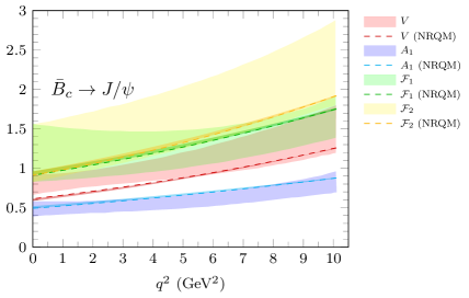
Figure 1: Comparison of the SM form factors for the $\bar{B}_{c}\to\eta_{c}$ (left) and $\bar{B}_{c}\to J/\psi$ (right) transitions, obtained with the NRQM calculation of Ref. Hernández et al. (2006) (dashed lines plus narrow uncertainty bands around them) and in the model independent analysis carried out in Ref. Cohen et al. (2019) (shown as bands). For a definition of the depicted form factors see Eqs. (2)–(3) and (7)–(9) of Ref. Cohen et al. (2019). As in Figs.6 and 7 of this latter reference, the dimension-full $f_{0}$ and ${\cal F}_{1}$ form-factors are given in units of $(M^{2}-M^{\prime\,2})$ and $\frac{1}{2}(M^{2}-M^{\prime\,2})$, respectively.

To evaluate the theoretical error associated to the Wilson coefficients for each of Fits 6 and 7, we use different sets of coefficients obtained through successive small steps in the multiparameter space, with each step leading to a moderate $\chi^{2}$ enhancement. We use 1$\sigma$ sets, i.e. values of the Wilson coefficients for which $\Delta\chi^{2}\leq 1$ with respect to its minimum value, to generate the distribution of each observable, taking into account in this way statistical correlations. From this derived distributions, we determine the maximum deviation above and below its central value, the latter obtained with the values of the Wilson coefficients corresponding to the minimum of $\chi^{2}$ and the AL1 form factors. These deviations define the, asymmetric in general, uncertainty associated with the NP Wilson coefficients. The two type of errors are then added in quadrature and they are shown in the figures as an extra, larger in size, uncertainty band.

The second set of form factors we shall use are the ones evaluated in Ref. Wang et al. (2013) within a perturbative QCD (pQCD) factorization approach. In this latter case only vector and axial-vector form factors have been obtained. They have been evaluated in the low $q^{2}$ region and extrapolated to higher $q^{2}$ values using a model dependent parameterization. These form factors have been used in the two recent calculations of Refs. Murgui et al. (2019); Watanabe (2018) where the rest of form factors needed (scalar, pseudoscalar or tensor ones) were determined using the quark level equations of motion of Ref. Sakaki et al. (2015). In Ref. Wang et al. (2013), the authors give the theoretical uncertainties for the vector and axial form factors at $q^{2}=0$. However neither correlations, nor errors for the parameters used in the $q^{2}-$extrapolation are provided. Besides, it is not clear what errors are introduced in the calculation through the use of the quark level equations of motion. Thus, in this case we will only show the error band stemming from the Wilson coefficients, even though larger uncertainties are to be expected.

As mentioned, for the $\bar{B}_{c}\to J/\psi$ decay, we shall compare our SM results with the ones reported in Ref. Harrison et al. (2020b), and obtained with the LQCD axial and vector form factors determined in Ref. Harrison et al. (2020a). In this case the $1\sigma$ uncertainty bands are obtained with the use of the correlation matrix provided in this latter reference.

II.1 Results with an unpolarized final $\tau$ lepton

We begin with the results corresponding to an unpolarized final $\tau$ lepton. In Fig. 2, we show the $d\Gamma/d\omega$ differential distribution for $\bar{B}_{c}\to\eta_{c}\tau\bar{\nu}_{\tau}$ and $\bar{B}_{c}\to J/\psi\tau\bar{\nu}_{\tau}$ reactions. As can be seen in the plots, the $\omega$ values accessible in the transitions are around $\omega\sim 1.2$ at most, while for the similar $\bar{B}\to D^{(*)}\tau\bar{\nu}_{\tau}$ reactions the available phase-space is larger, and $\omega$ varies from 1 to 1.35–1.40.

In both $\bar{B}_{c}$ decays, the NRQM form factors from Ref. Hernández et al. (2006) lead to larger total widths. Looking at the SM results for the $\bar{B}_{c}\to J/\psi$ decay, one sees that the LQCD prediction from Ref. Harrison et al. (2020b) is in between the NRQM and pQCD distribution, somewhat closer to the former one, but still showing a tension of around $2\sigma$ in most of the phase space. Since relativistic effects increase as one departs from zero-recoil to $q^{2}=0$, they might be responsible for some of the NRQM-LQCD discrepancies exhibited in the figure far from the vicinity of $\omega=1$.

For the decay into $\eta_{c}$ computed with the NRQM form factors we note that already $d\Gamma/d\omega$ discriminate between NP Fits 6 and 7. For the rest of cases shown in the figure, though NP effects are clearly visible, we see that this observable would not be able to distinguish between the two NP scenarios examined in this work.

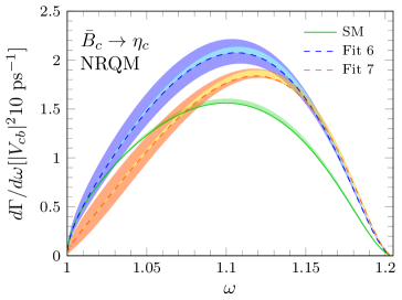
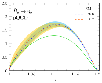
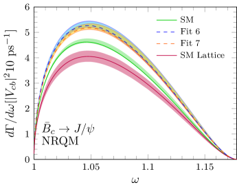
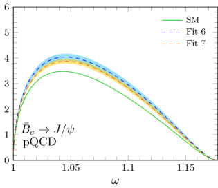
Figure 2: Top: $d\Gamma(\bar{B}_{c}\to\eta_{c}\tau\bar{\nu}_{\tau})/d\omega$ differential decay width, as a function of $\omega$ and in units of $10|V_{cb}|^{2}{\rm ps}^{-1}$. We show SM predictions and full NP results obtained using the Wilson coefficients from Fits 6 and 7 of Ref. Murgui et al. (2019) and form factors from the NRQM (left panel) and the pQCD (right panel) approaches of Refs. Hernández et al. (2006) and Wang et al. (2013), respectively. Bottom: Same as before but for the $\bar{B}_{c}\to J/\psi\tau\bar{\nu}_{\tau}$ decay. In the left-bottom plot, we also show the SM lattice result from Ref. Harrison et al. (2020b). Uncertainty bands obtained as detailed in the main text.

	SM			NP Fit 6		NP Fit 7
	[NRQM]	[pQCD]	[HPQCD]	[NRQM]	[pQCD]	[NRQM]	[pQCD]
${\cal R}_{\eta_{c}}=\frac{\Gamma(\bar{B}_{c}\to\eta_{c}\tau\bar{\nu}_{\tau})}{\rule{0.0pt}{6.02777pt}\Gamma(\bar{B}_{c}\to\eta_{c}\mu\bar{\nu}_{\mu})}$	$0.349^{+0.000}_{-0.007}$	0.309		$0.452^{+0.034}_{-0.030}$	$0.40^{+0.03}_{-0.03}$	$0.384^{+0.024}_{-0.018}$	$0.40^{+0.04}_{-0.03}$
${\cal R}_{J/\psi}=\frac{\Gamma(\bar{B}_{c}\to J/\psi\tau\bar{\nu}_{\tau})}{\rule{0.0pt}{6.02777pt}\Gamma(\bar{B}_{c}\to J/\psi\mu\bar{\nu}_{\mu})}$	$0.266^{+0.000}_{-0.004}$	0.289	$0.2601\pm 0.0036$	$0.306^{+0.007}_{-0.007}$	$0.342^{+0.013}_{-0.015}$	$0.301^{+0.005}_{-0.007}$	$0.326^{+0.008}_{-0.009}$

Table 1: ${\cal R}_{\eta_{c}}$ and ${\cal R}_{J/\psi}$ ratios obtained in the SM and with NP effects from Ref. Murgui et al. (2019). We give results using the [NRQM] Hernández et al. (2006) and [pQCD] Wang et al. (2013) sets of form-factors, and additionally ${\cal R}_{J/\psi}^{\rm SM}$ from the LQCD analysis carried out by the HPQCD collaboration Harrison et al. (2020b).

Evaluating the SM predictions for a final massless charged lepton ($\mu$ or $e$), we obtain the ${\cal R}_{\eta_{c}}$ and ${\cal R}_{J/\psi}$ ratios collected in Table 1. The systematic uncertainties due to the inter-quark potential in the NRQM scheme are largely canceled out in the ratios, as can be inferred from the SM predictions. For the SM we find a nice agreement of the NRQM determination of ${\cal R}_{J/\psi}$ and the lattice evaluation of Ref. Harrison et al. (2020b), pointing out also to a compensation in the ratio of the overall-normalization discrepancies noted in Fig. 2. On the other hand, predictions with the NRQM and pQCD form factors differ by approximately 10%, except for NP Fit 7 ${\cal R}_{\eta_{c}}$, where the change is only of 4%. In fact, the form-factor systematic uncertainties are reduced compared to those observed in some regions of the differential distributions in Fig. 2. We also note that the NRQM ${\cal R}_{\eta_{c}}$ and ${\cal R}_{J/\psi}$ ratios are systematically bigger and smaller, respectively, than those obtained with pQCD form factors. For the latter ratio, we mentioned above that $\Gamma^{\rm NRQM}(\bar{B}_{c}\to J/\psi\tau\bar{\nu}_{\tau})\geq\Gamma^{\rm pQCD}(\bar{B}_{c}\to J/\psi\tau\bar{\nu}_{\tau})$ and thus, the massless lepton modes of the $\bar{B}_{c}\to J/\psi$ semileptonic decay calculated with NRQM form factors must also be larger than when pQCD form factors are used. Moreover, the difference has to be greater than for the $\tau$ mode to explain $R^{\rm NRQM}_{J/\psi}\leq R^{\rm pQCD}_{J/\psi}$.

The ratios including NP are greater than pure SM expectations, around 30% and 15% for ${\cal R}_{\eta_{c}}$ and ${\cal R}_{J\psi}$, respectively, except for the NRQM ${\cal R}_{\eta_{c}}$ case evaluated with the NP Fit 7 where an increase of only 10% is found. In fact, at the level of ratios, only the NRQM ${\cal R}_{\eta_{c}}$ discriminates between NP Fits 6 and 7. One can compare the values for ${\cal R}_{J/\psi}$ with the only available experimental measurement quoted above. In this case we see all predictions fall short of the present central experimental value by almost $2\sigma$, adding in quadratures the errors given in Eq. (2). The agreement is slightly better when using the pQCD form-factor set. The improvement is not significant, however, within the present accuracy in the data and, as we explain below, there are some inconsistencies in the corresponding pQCD form factors for this decay.

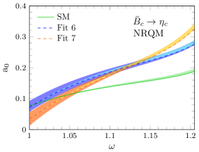
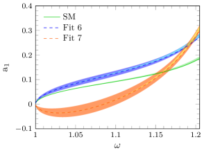
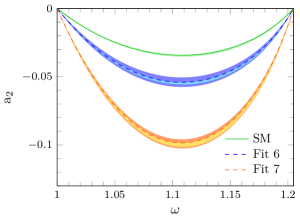
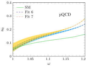
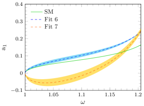
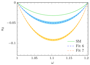
Figure 3: $\bar{B}_{c}\to\eta_{c}\tau\bar{\nu}_{\tau}$ decay: CM $a_{0,1,2}$ angular expansion coefficients as a function of $\omega$. We show results obtained with both, NRQM (upper panels) and pQCD (lower panels) form factors from Refs. Hernández et al. (2006) and Wang et al. (2013), respectively. The beyond of the SM scenarios Fits 6 and 7 are taken from Ref. Murgui et al. (2019). Uncertainty bands as in Fig. 2.

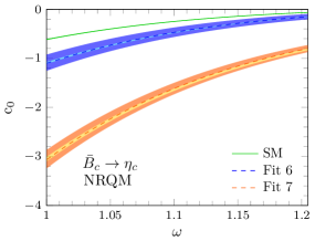
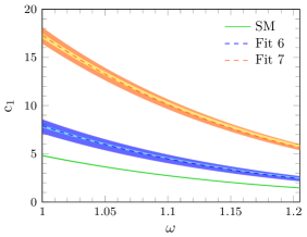
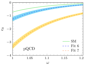
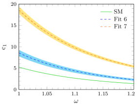
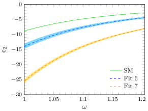
Figure 4: $\bar{B}_{c}\to\eta_{c}\tau\bar{\nu}_{\tau}$ decay: Same as in Fig. 3 but for the LAB $c_{0,1,2}$ energy expansion coefficients.

Now we discuss results for the $d^{2}\Gamma/(d\omega d\cos\theta_{\ell})$ and $d^{2}\Gamma/(d\omega dE_{\ell})$ double differential distributions. The $a_{0,1,2}$ CM angular and $c_{0,1,2}$ LAB energy expansion coefficients are shown in Figs. 3 and 4, and Figs. 5 and 6 for the $\eta_{c}$ and $J/\psi$ decay modes, respectively.

For the $\bar{B}_{c}\to\eta_{c}\tau\bar{\nu}_{\tau}$ decay, both sets of form factors lead to qualitatively very similar results. As in Ref. Penalva et al. (2020) for the $\Lambda_{b}\to\Lambda_{c}\tau\bar{\nu}_{\tau}$ semileptonic decay, we find that, with the exception of $a_{0}$, all the other expansion coefficients serve the purpose of giving a clear distinction between NP Fits 6 and 7. Thus, different fits that otherwise give similar $d\Gamma/d\omega$ decay widths, can be told apart by looking at these CM angular or LAB energy observables. In addition, we also observe $\omega-$shapes for all $\bar{B}_{c}\to\eta_{c}$ SM and NP coefficients similar to those obtained in Ref. Penalva et al. (2020) for the $\Lambda_{b}\to\Lambda_{c}$ transition, except $a_{0}$ that here grows with $\omega$ while for the baryon decay it is a decreasing function of $\omega$.

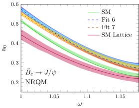
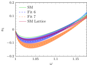
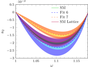
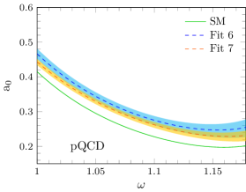
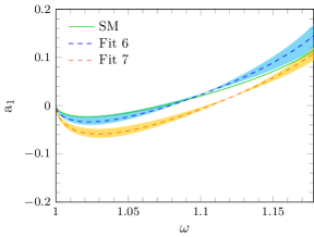
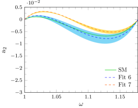
Figure 5: $\bar{B}_{c}\to J/\psi\tau\bar{\nu}_{\tau}$ decay: CM $a_{0,1,2}$ angular expansion coefficients as a function of $\omega$. We show results obtained with both, NRQM (upper panels) and pQCD (lower panels) form factors from Refs. Hernández et al. (2006) and Wang et al. (2013), respectively. In the upper panels, SM results for these observables obtained with the LQCD form-factors reported in Ref. Harrison et al. (2020a) are also displayed. The beyond of the SM scenarios Fits 6 and 7 are taken from Ref. Murgui et al. (2019). Uncertainty bands as in Fig. 2.

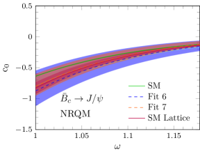
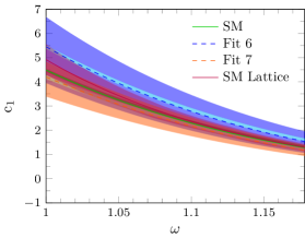
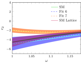
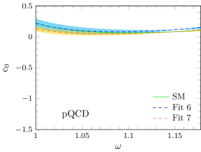
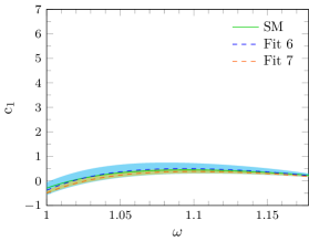
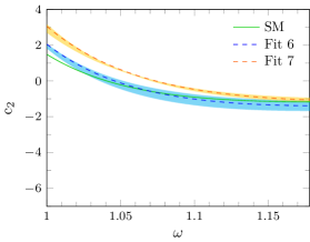
Figure 6: $\bar{B}_{c}\to J/\psi\tau\bar{\nu}_{\tau}$ decay: Same as in Fig. 5 but for the LAB $c_{0,1,2}$ energy expansion coefficients.

The corresponding results for a decay into $J/\psi$ are shown in Figs. 5 and 6. There are two distinct features in this case. First, the utility of these observables to distinguish between Fits 6 and 7 and, in some cases, between those NP predictions and the SM results, is not as good as in the $\eta_{c}$ case. This happens to be true independent of the form-factor set used. Second, the results obtained with the two form-factor sets turn out to be very different in most cases, with only $a_{0}$ and $a_{1}$ showing a similar qualitative behavior. By looking at SM results alone we find a good qualitative agreement between NRQM and LQCD results while, with the exception of $a_{0}$ and $a_{1}$, we find very different shapes for the results obtained using the pQCD form factors. In order to better understand this discrepancy, we show in Fig. 7 all the form factors defined in Eqs. (16) and (17), for decays into both $\eta_{c}$ and $J/\psi$. In the left panel we give the results obtained with the AL1 NRQM of Ref. Hernández et al. (2006). We see the results are close to expectations from Eq. (22) based on HQSS. In the middle panel we give the results obtained using the form factors from Ref. Wang et al. (2013) and the quark level equations of motion from Ref. Sakaki et al. (2015). Large violations of HQSS are already seen for $h_{A_{2}}$ and $h_{A_{3}}$ (where no quark level equations of motion are involved), also for $h_{T_{3}}$ and, to a lesser extent, for $h_{P}$. These HQSS violations are related, at least in part, to the fact that the $A_{0}(q^{2}),A_{1}(q^{2})$ and $A_{2}(q^{2})$ axial form factors evaluated in Ref. Wang et al. (2013), and in terms of which the $h_{A_{1,2,3}}$ ones are determined, do not respect the $q^{2}=0$ constraint

$$A_{0}(0)=\frac{M+M^{\prime}}{2M^{\prime}}A_{1}(0)-\frac{M-M^{\prime}}{2M^{\prime}}A_{2}(0)$$ (7)

Even though $q^{2}\geq m_{\tau}^{2}$ for a final $\tau$, taking the wrong values of the form factors at $q^{2}=0$ affects the determination of the values at larger $q^{2}$. In the right panel of Fig. 7 we see the effect of imposing the above constraint on $A_{0}(0)$. The $h_{P}$ form factor is now in agreement with HQSS expectations and things improve for $h_{A_{2}},h_{A_{3}}$ and $h_{T_{3}}$. Note that this restriction also corrects the divergences at $q^{2}=0$ that otherwise appear for $h_{A_{2}}$ and $h_{A_{3}}$ and which signatures are clearly visible in the middle panel at large recoils. Moreover, with this restriction imposed, the results for ${\cal R}_{J/\psi}$ would get smaller, $0.311^{+0.007}_{-0.006}$ for Fit 6 and $0.303^{+0.005}_{-0.004}$ for Fit 7, and in much better agreement with the ones obtained using the NRQM form factors from Ref. Hernández et al. (2006) (see Table 1). Besides, and though they are less important numerically, there are divergences in all three $h_{T_{1,2,3}}$ form factors at $q^{2}=0$ when quark-level equations of motion are used to obtain them. The beginning of these divergences can already be seen in the middle and right panels of Fig. 7.

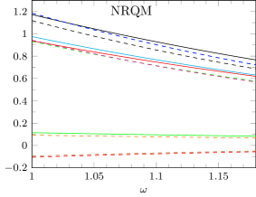
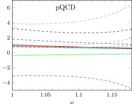
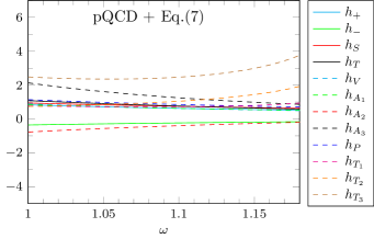
Figure 7: Different $h_{a}$ form factors defined in Eqs. (16) and (17) for $\bar{B}_{c}\to\eta_{c}$ and $\bar{B}_{c}\to J/\psi$ semileptonic decays. Left panel: Results obtained with the NRQM of Ref. Hernández et al. (2006) using the AL1 potential. Middle panel: Results obtained from the form factors of Ref. Wang et al. (2013) and the use of quark-level equations of motion from Ref. Sakaki et al. (2015). Right panel: Same as the middle panel but forcing Eq. (7) on $A_{0}(0)$.

In Fig. 8 we now show the forward-backward asymmetry in the CM frame evaluated with the form factors from the NRQM of Ref. Hernández et al. (2006). This asymmetry is given by the ratio

$${\cal A}_{FB}=\frac{a_{1}(\omega)}{2a_{0}(\omega)+2a_{2}(\omega)/3}$$ (8)

For the decay into $J/\psi$, SM results for this asymmetry from the LQCD form-factors of Ref. Harrison et al. (2020a) are also shown. Note that ${\cal A}_{FB}$ is given in Harrison et al. (2020b) as well. For this decay mode, as it is also the case for other observables, the SM result falls into the error band of Fit 6. However, for both $\bar{B}_{c}\to\eta_{c}$ and $\bar{B}_{c}\to J/\psi$ transitions, this observable is also able to distinguish between Fits 6 and 7, in particular for the $\eta_{c}$ channel.

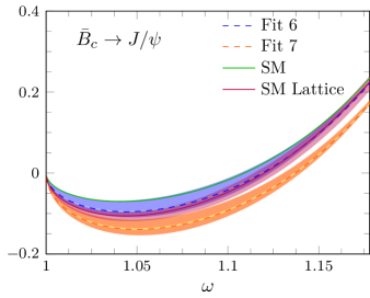
Figure 8: Forward-backward asymmetry in the CM reference frame for the $\bar{B}_{c}\to\eta_{c}\tau\bar{\nu}_{\tau}$ (left) and $\bar{B}_{c}\to J/\psi\tau\bar{\nu}_{\tau}$ (right) decays. The results have been obtained with the form factors evaluated with the NRQM of Ref. Hernández et al. (2006). For the $\bar{B}_{c}\to J/\psi$ case, we also show the SM prediction from the LQCD results of Ref. Harrison et al. (2020b). Uncertainty bands as in Fig. 2.

II.2 Results with a polarized final $\tau$ lepton

In this section we collect the results corresponding to the $\bar{B}_{c}\to\eta_{c}\tau\bar{\nu}_{\tau}$ and $\bar{B}_{c}\to J/\psi\tau\bar{\nu}_{\tau}$ decays with a polarized $\tau$ (well defined helicity $h=\pm 1$ in the CM or LAB frames). In this case, and for simplicity, we will only present results obtained with the use of the NRQM form factors from Ref. Hernández et al. (2006), and, for the $\bar{B}_{c}\to J/\psi$ case, also the SM results obtained with the LQCD form factors from Ref. Harrison et al. (2020a). In Fig. 9 we show the $d\Gamma/d\omega$ differential decay width for the $\bar{B}_{c}\to\eta_{c}\tau\bar{\nu}_{\tau}$ decay with a final $\tau$ with well defined helicity in the CM reference frame (left panel) and in the LAB system (right panel). The corresponding results for the $\bar{B}_{c}\to J/\psi\tau\bar{\nu}_{\tau}$ decay are presented in Fig. 10. The negative helicity contribution is dominant in all cases except for the $\eta_{c}$ CM distributions obtained both in the SM and in Fit 6. This unexpected feature also occurs for the polarized $\bar{B}\to D\tau\bar{\nu}_{\tau}$ decay (see Appendix D). We see that both CM and LAB $\tau$ negative-helicity distributions obtained in $\eta_{c}$ decays clearly discriminate between SM and different NP scenarios. On the other hand, for the $\bar{B}_{c}\to J/\psi\tau\bar{\nu}_{\tau}$ decay $d\Gamma/d\omega$ is not an efficient tool for that purpose, even taking into account information on the outgoing $\tau-$polarization. As we noted in Fig. 2 for the unpolarized $d\Gamma/d\omega$, the LQCD results Harrison et al. (2020a) for the SM $\tau$ negative-helicity CM and LAB $\bar{B}_{c}$ distributions are around $2\sigma$ below the NRQM predictions, while the shapes turn out to be in excellent agreement.

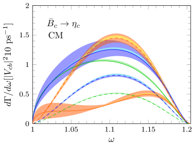
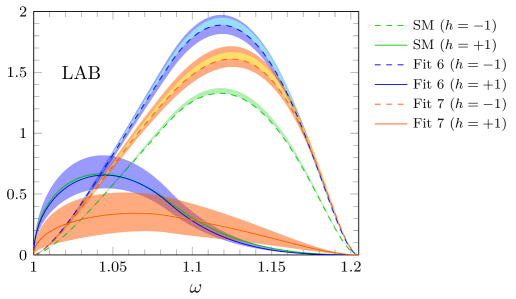
Figure 9: CM (left) and LAB (right) helicity decomposition of the $d\Gamma(\bar{B}_{c}\to\eta_{c}\tau\bar{\nu}_{\tau})/d\omega$ differential decay width, calculated with the NRQM form factors from Ref. Hernández et al. (2006). Uncertainty bands as in Fig. 2.

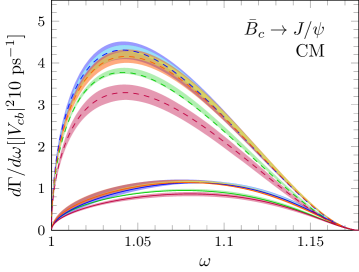
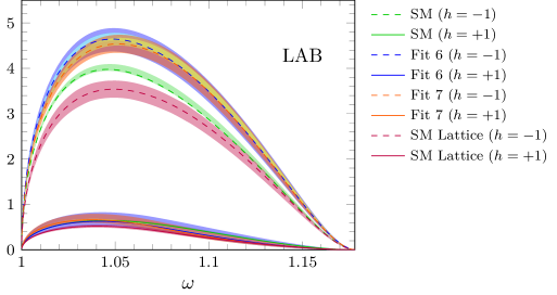
Figure 10: As in Fig. 9, but for the $\bar{B}_{c}\to J/\psi\tau\bar{\nu}_{\tau}$ decay. We also show the SM results obtained with LQCD form factors from Ref. Harrison et al. (2020a).

As shown in Ref. Penalva et al. (2020), for a polarized final $\tau$ lepton with well defined helicity $h=\pm 1$, the CM angular and LAB energy distributions are respectively determined by

$$\frac{2\overline{\sum}|{\cal M}|^{2}}{M^{2}(1-\frac{m_{\ell}^{2}}{q^{2}})}=a_{0}(\omega,h)+a_{1}(\omega,h)\cos\theta_{\ell}+a_{2}(\omega,h)(\cos\theta_{\ell})^{2}$$ (9)

$$\frac{2\overline{\sum}|{\cal M}|^{2}}{M^{2}}=\frac{1}{2}\left(c_{0}+c_{1}\frac{E_{\ell}}{M}+c_{2}\frac{E^{2}_{\ell}}{M^{2}}\right)-\frac{h}{2}\frac{M}{p_{\ell}}\left(\widehat{c}_{0}+\left[c_{0}+\widehat{c}_{1}\right]\frac{E_{\ell}}{M}+\left[c_{1}+\widehat{c}_{2}\right]\frac{E^{2}_{\ell}}{M^{2}}+\left[c_{2}+\widehat{c}_{3}\right]\frac{E^{3}_{\ell}}{M^{3}}\right)$$ (10)

In the latter equation, $p_{\ell}$ is the modulus of the final charged lepton three-momentum measured in the LAB frame. The general expressions of the $a_{0,1,2}(\omega,h)$ and $\widehat{c}_{0,1,2,3}(\omega)$ coefficients in terms of the $\widetilde{W}$ SFs can be found in Ref. Penalva et al. (2020).

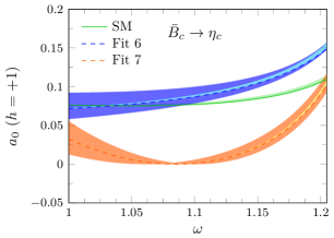
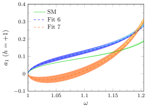
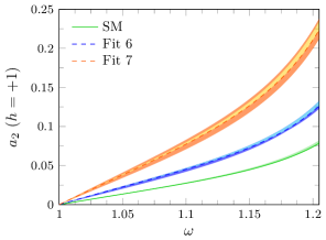
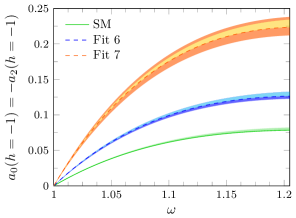
Figure 11: CM angular expansion coefficients for the $\bar{B}_{c}\to\eta_{c}\tau\bar{\nu}_{\tau}$ decay with a polarized $\tau$ with positive (upper panels) and negative (lower panels) helicity. They have been evaluated with the NRQM form factors from Ref. Hernández et al. (2006). Uncertainty bands as in Fig. 2.

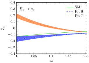
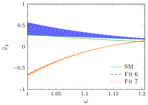
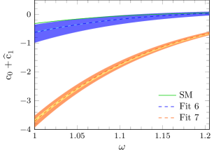
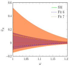
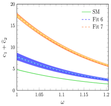
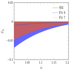
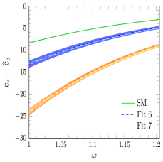
Figure 12: LAB charged lepton energy expansion coefficients $\widehat{c}_{0,1,2,3}(\omega)$ for the polarized $\bar{B}_{c}\to\eta_{c}\tau\bar{\nu}_{\tau}$ decay. We also show the $(c_{0}+\widehat{c}_{1})$, $(c_{1}+\widehat{c}_{2})$ and $(c_{2}+\widehat{c}_{3})$ sums in the third top, second and fourth bottom panels, respectively. All the functions have been evaluated with the NRQM form factors from Ref. Hernández et al. (2006). Uncertainty bands as in Fig. 2.

In Figs. 11 and 12 we present the results for the functions $a_{0,1,2}(\omega,h=\pm 1)$ (CM) and $\widehat{c}_{0,1,2,3}(\omega)$ (LAB) for the polarized $\bar{B}_{c}\to\eta_{c}\tau\bar{\nu}_{\tau}$ reaction.

We see that even taking uncertainties into account, Fits 6 and 7 provide distinct predictions for all non-zero angular coefficients that also differ from the SM results, with the exception of $a_{0}(\omega,h=+1)$, for which SM and NP Fit 6 results overlap below $\omega\leq 1.1$. We also observe that for this decay ($\bar{B}_{c}\to\eta_{c}$), the relations

$$a_{0}(\omega,h=-1)=-a_{2}(\omega,h=-1),\qquad a_{1}(\omega,h=-1)=0$$ (11)

are satisfied because of angular momentum conservation. Since both the initial and final hadrons have zero spin, the virtual particle exchanged (a $W$ boson in the SM) should have helicity zero. In the CM system this corresponds to a zero spin projection along the quantization axis defined by its three-momentum in the LAB frame, the same axis that is defined by the final hadron LAB (or CM) three-momentum. Thus, in the CM system, the angular momentum of the final lepton pair measured along that axis must be zero. As a consequence, the CM helicity of a final $\tau$ lepton emitted along that direction, which corresponds to either $\theta_{\ell}=0$ or $\theta_{\ell}=\pi$, must equal that of the $\bar{\nu}_{\tau}$, the latter being always positive. This means that a negative helicity $\tau$ can not be emitted in the CM system when $\theta_{\ell}=0$ or $\pi$. Looking at Eq. (9), this implies that $a_{0}(\omega,h=-1)=-a_{2}(\omega,h=-1)$ and $a_{1}(\omega,h=-1)=0$.

Besides, at zero recoil CM and LAB frames coincide and angular momentum conservation requires the helicity of the $\tau$ lepton to equal that of the anti-neutrino. This implies $a_{0}(\omega=1,h=-1)=-a_{2}(\omega=1,h=-1)=0$, and also the cancellation of Eq. (10) at zero recoil for $h=-1$. In fact, the LAB $d^{2}\Gamma(\bar{B}_{c}\to\eta_{c}\tau\bar{\nu}_{\tau})/(d\omega dE_{\ell})$ distribution should cancel for $h=-1$ and any value of $\omega$ when $E_{\ell}$ equals its maximum value for that particular $\omega$. The reason is that this maximum $E_{\ell}$ value corresponds necessarily to $\theta_{\ell}=\pi$ and in that case the helicity of the $\tau$ is the same in both CM and LAB frames. Since $h=-1$ is forbidden in the CM for that specific kinematics it is also forbidden in the LAB. Note that any violation of these results will require negative helicity anti-neutrinos which means NP contributions with right-handed neutrinos. The possible role of such beyond the SM terms in the explanation of the LFU ratio anomalies have been considered in Refs. Ligeti et al. (2017); Asadi et al. (2018); Greljo et al. (2018); Robinson et al. (2019); Azatov et al. (2018); Heeck and Teresi (2018); Asadi et al. (2019); Babu et al. (2019); Bardhan and Ghosh (2019); Shi et al. (2019); Gómez et al. (2019) and their existence has not been discarded by the available $\bar{B}\to D^{(*)}$ data Mandal et al. (2020).

Note also that, as a result of $a_{1}(\omega,h=-1)$ being zero for the $P_{b}\to P_{c}$ decays, the forward-backward asymmetry in the CM system (${\cal A}_{FB}$ shown in the left panel of Fig. 8) can only originate from positive helicity $\tau$’s. For the same reason, for massless charged leptons ($\ell=e,\mu$), ${\cal A}_{FB}$ vanishes in the SM for transitions between pseudoscalar mesons.

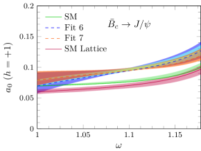
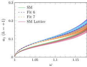
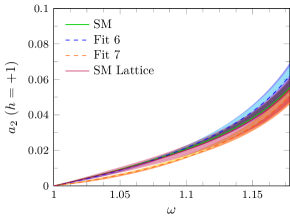
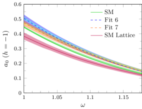
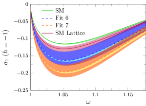
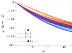
Figure 13: CM angular expansion coefficients for the $\bar{B}_{c}\to J/\psi\tau\bar{\nu}_{\tau}$ decay with a $\tau$ with positive (upper panels) and negative (lower panels) helicity. They have been evaluated with the NRQM form factors from Ref. Hernández et al. (2006). We also show the SM results obtained with LQCD form factors from Ref. Harrison et al. (2020a). Uncertainty bands as in Fig. 2.

Looking at positive helicities, one finds that, in the high $\omega$ region, the quantity $a_{0}(\omega,h=+1)-a_{1}(\omega,h=+1)+a_{2}(\omega,h=+1)$ shows a steady decrease, as $\omega$ increases. In fact, at maximum recoil, one has the approximate result

$$a_{0}(\omega_{\rm max},h=+1)-a_{1}(\omega_{\rm max},h=+1)+a_{2}(\omega_{\rm max},h=+1)\approx 0,$$ (13)

that can be readily inferred from the corresponding figures and which corresponds to a very small probability of CM positive helicity $\tau$’s emitted at $\theta_{\ell}=\pi$ when $\omega=\omega_{\rm max}$. This result can be partially understood taking into account that our main contribution selects negative chirality for the final charged lepton. A $\tau$ lepton emitted with positive helicity in the CM frame and with $\theta_{\ell}=\pi$ will also have positive helicity in the LAB frame. However, close to maximum recoil its momentum in the LAB is very large and helicity almost equals chirality, hence the partial cancellation. Note that this result would be independent of the spin of the hadrons involved as long as negative chirality lepton current operators are dominant. This approximate relation in Eq. (13) can already be seen in the polarized results for the $\Lambda_{b}\to\Lambda_{c}$ decay shown in Ref. Penalva et al. (2020). Besides, and for the same chirality/helicity argument, one expects the LAB ratio $\frac{d\Gamma/d\omega(h=+1)}{d\Gamma/d\omega(h=-1)}$ to be small in the high $\omega$ region, the reason being that for $\omega$ close to $\omega_{\rm max}$ the charged lepton energies are significantly larger than its mass.

In Fig. 12 we present the results for the $\widehat{c}_{0,1,2,3}(\omega)$ coefficients associated to this decay. We observe that $\widehat{c}_{0}(\omega)$ and $\widehat{c}_{1}(\omega)$ are able to distinguish between the two NP fits from Ref. Murgui et al. (2019) considered in the present work. The other two observables $\widehat{c}_{2}(\omega)$ and $\widehat{c}_{3}(\omega)$, available from the polarized $d^{2}\Gamma(\bar{B}_{c}\to\eta_{c}\tau\bar{\nu}_{\tau})/(d\omega dE_{\ell})$ distribution, turn out to be very small and negligible when compared with $c_{1}$ and $c_{2}$, respectively (see the plots in Fig. 12). Therefore, these two additional coefficients have little relevance in the discussion of the NP Fits 6 and 7, for which the NP tensor Wilson coefficient $|C_{T}|\sim 10^{-2}$ is quite small. As discussed in Ref. Penalva et al. (2020), $\widehat{c}_{2}$ and $\widehat{c}_{3}$ are, however, optimal observables to restrict the validity of NP schemes with larger $|C_{T}|$ values.

In Figs. 13 and 14 we collect the corresponding results for the $\bar{B}_{c}\to J/\psi\tau\bar{\nu}_{\tau}$ decay. In this case, no angular momentum related restriction is in place for $a_{0,1,2}(\omega,h=-1)$ since the final hadron has spin one and there are three possible helicity states. However, one can see that the approximate relation in Eq. (13) is indeed satisfied. Also the discussion above about the LAB ratio $\frac{d\Gamma/d\omega(h=+1)}{d\Gamma/d\omega(h=-1)}$ being small near maximum recoil also applies for this decay. When looking at SM results alone we find a qualitative agreement of NRQM and LQCD results.

To conclude this section, in Fig. 15 we present the results for the $\tau$ polarization asymmetry

$${\cal A}_{\lambda_{\tau}}=\frac{d\Gamma/d\omega(h=-1)-d\Gamma/d\omega(h=+1)}{d\Gamma/d\omega(h=-1)+d\Gamma/d\omega(h=+1)}$$ (14)

measured both in the CM and LAB frames.

For the $\bar{B}_{c}\to\eta_{c}$ decay we see that both polarization asymmetries equal minus one at zero recoil and that the LAB one tends to plus one when maximum recoil is approached. The Wilson coefficients of the charged-lepton positive chirality ${\cal O}_{S_{L},S_{R}}$ operators in the Fit 7 are significantly larger than in the Fit 6, which explains the larger deviations of ${\cal A}_{\lambda_{\tau}}$ from $+1$ at $\omega=\omega_{\rm max}$ in the first NP scenario. This is in perfect accordance with the discussion above. As it is clear from the figure, the CM polarization asymmetry is a good observable to distinguish between different NP scenarios. This is not the case however of the LAB one. For the $\bar{B}_{c}\to J/\psi$ decay the asymmetries are equal at zero recoil, since CM and LAB frames coincide at $\omega=1$, but otherwise they show a very different $\omega$ dependence. None of them is able to distinguish NP results for Fits 6 and 7 among themselves and from the SM. We also observe for these latter decays, a quite good agreement between NRQM and LQCD predictions in particular for the results found in the CM frame, which are also reported in the recent analysis of Ref. Harrison et al. (2020b).

Although the $\bar{B}_{c}\to J/\psi$ decay is perhaps easier to measure experimentally, as a general rule we find the $\bar{B}_{c}\to J/\psi$ observables, also in the case of a polarized $\tau$, are less optimal for distinguishing between NP Fits 6 and 7 than those discussed above for $\bar{B}_{c}\to\eta_{c}$ decays, or those presented in Ref. Penalva et al. (2020) for the related $\Lambda_{b}\to\Lambda_{c}$ semileptonic decay.

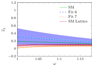
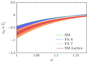
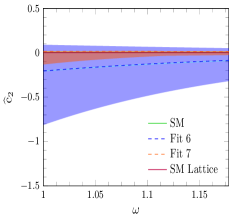
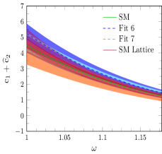
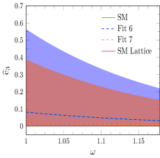
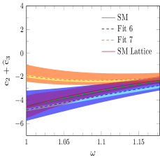
Figure 14: LAB charged lepton energy expansion coefficients $\widehat{c}_{0,1,2,3}(\omega)$ for the polarized $\bar{B}_{c}\to J/\psi\tau\bar{\nu}_{\tau}$ decay. We also show the $(c_{0}+\widehat{c}_{1})$, $(c_{1}+\widehat{c}_{2})$ and $(c_{2}+\widehat{c}_{3})$ sums in the third top, second and fourth bottom panels, respectively. All the functions have been evaluated with the NRQM form factors from Ref. Hernández et al. (2006). We also show the SM results obtained with LQCD form factors from Ref. Harrison et al. (2020a). Uncertainty bands as in Fig. 2.

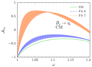
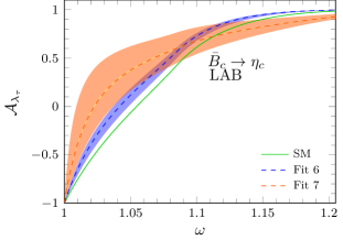
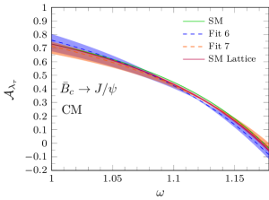
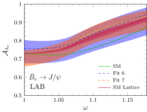
Figure 15: $\tau$ polarization asymmetry ${\cal A}_{\lambda_{\tau}}$, defined in Eq. (14), for the $\bar{B}_{c}\to\eta_{c}$ (upper panels) and $\bar{B}_{c}\to J/\psi$ (lower panels) semileptonic decays measured in the CM (left panels) and LAB (right panels) frames. They have been obtained with the NRQM form factors from Ref. Hernández et al. (2006). For the $\bar{B}_{c}\to J/\psi$ case we also show the SM results obtained with the LQCD form factors from Ref. Harrison et al. (2020a). Uncertainty bands as in Fig. 2.

III $\bar{B}\to D$ and $\bar{B}\to D^{*}$ semileptonic decay results with an unpolarized final $\tau$ lepton

We present now results for the $\bar{B}\to D\tau\bar{\nu}_{\tau}$ and $\bar{B}\to D^{*}\tau\bar{\nu}_{\tau}$ semileptonic decays. As in the previous section, we shall use the Wilson coefficients and form factors corresponding to Fits 6 and 7 in Ref. Murgui et al. (2019). The form factors are taken from Ref. Bernlochner et al. (2017), but in Ref. Murgui et al. (2019) not only the Wilson coefficients but also the $1/m_{b,c}$ and $1/m^{2}_{c}$ corrections to the form factors are simultaneously fitted to experimental data. To estimate the theoretical uncertainties, for each fit, we shall use different sets of Wilson coefficients and form factors, selected such that the $\chi^{2}$ merit function computed in Murgui et al. (2019) changes at most by one unit from its value at the fit minimum. With those sets, for each of the observables that we calculate we determine the maximum deviations above and below their central values. These deviations will give us the $1\sigma$ theoretical uncertainty and it will be shown as an error band in the figures below.

We start by showing in Fig. 16 the $d\Gamma/d\omega$ differential decay width. Both NP fits give similar results that differ from the SM distribution.

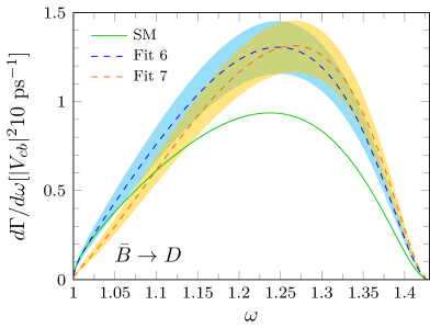
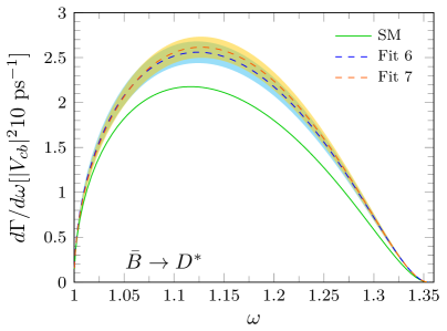
Figure 16: $d\Gamma(\bar{B}\to D\tau\bar{\nu}_{\tau})/d\omega$ (left) and $d\Gamma(\bar{B}\to D^{*}\tau\bar{\nu}_{\tau})/d\omega$ (right) differential decay widths, as a function of $\omega$ and in units of $10|V_{cb}|^{2}{\rm ps}^{-1}$. We show SM predictions and full NP results obtained using the Wilson coefficients and form factors corresponding to Fits 6 and 7 of Ref. Murgui et al. (2019). Uncertainty bands obtained as explained in the main text.

The corresponding predictions for the ${\cal R}_{D}$ and ${\cal R}_{D^{*}}$ ratios are given in Table 2.

	SM	Fit 6	Fit 7
${\cal R}_{D}=\frac{\Gamma(\bar{B}\to D\tau\bar{\nu}_{\tau})}{\rule{0.0pt}{6.02777pt}\Gamma(\bar{B}\to D\ell\bar{\nu}_{\ell})}$	$0.300\pm 0.005$	$0.405\pm 0.048$	$0.389\pm 0.045$
${\cal R}_{D^{*}}=\frac{\Gamma(\bar{B}\to D^{*}\tau\bar{\nu}_{\tau})}{\rule{0.0pt}{6.02777pt}\Gamma(\bar{B}\to D^{*}\ell\bar{\nu}_{\ell})}$	$0.251\pm 0.004$	$0.302\pm 0.014$	$0.306\pm 0.013$

Table 2: ${\cal R}_{D}$ and ${\cal R}_{D^{*}}$ ratios obtained in the SM and with NP effects from Ref. Murgui et al. (2019)).

The ratios obtained with NP are in agreement with present experimental results, though they are located at the high-value corner of the allowed regions, since they were fitted in Ref. Murgui et al. (2019) to the previous HFLAV world average values quoted in Amhis et al. (2017). Again, we notice that for these quantities both fits are equivalent within errors and other observables are needed in order to decide between different NP explanations of the experimental data.

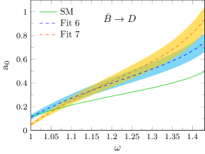
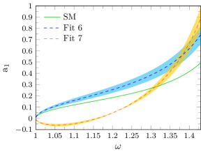
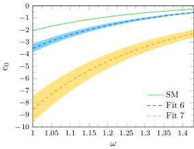
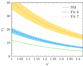
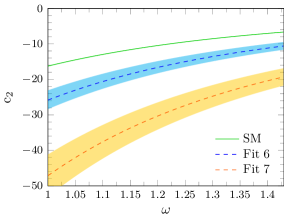
Figure 17: $\bar{B}\to D\tau\bar{\nu}_{\tau}$ decay: $a_{0,1,2}$ CM angular and $c_{0,1,2}$ LAB energy expansion coefficients as a function of $\omega$. Uncertainty bands as in Fig. 16.

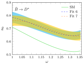
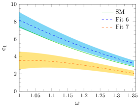
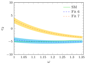
Figure 18: $\bar{B}\to D^{*}\tau\bar{\nu}_{\tau}$ decay: $a_{0,1,2}$ CM angular and $c_{0,1,2}$ LAB energy expansion coefficients as a function of $\omega$. Uncertainty bands as in Fig. 16.

These observables can be the $a_{0,1,2}$ and $c_{0,1,2}$ coefficients in the CM angular $d^{2}\Gamma/(d\omega d\cos\theta_{\ell})$ and LAB energy $d^{2}\Gamma/(d\omega dE_{\ell})$ distributions. They are shown in Figs. 17 and 18 for the $\bar{B}\to D\tau\bar{\nu}_{\tau}$ and $\bar{B}\to D^{*}\tau\bar{\nu}_{\tau}$ decays, respectively. With the only exception of $a_{0}$, all of them can be used to distinguish between the two fits. However, for the $\bar{B}\to D^{*}$, and similar to what happened for the $\bar{B}_{c}\to J/\psi$ decay, SM results for some of these coefficients fall within the error band of those obtained from NP Fit 6. In fact the $\omega-$shape patterns exhibited in Figs. 17 and 18 for the $\bar{B}\to D^{(*)}$ reactions are qualitatively similar to those found in Sec. II for the $\bar{B}_{c}$ decays.

We stress that the LAB $d^{2}\Gamma(\bar{B}\to D^{(*)}\tau\bar{\nu}_{\tau})/(d\omega dE_{\ell})$ differential decay widths are reported for the very first time in this work. Though, as shown in Penalva et al. (2020), CM and LAB unpolarized distributions provide access to equivalent dynamical information (invariant functions ${\cal A(\omega)}$, ${\cal B(\omega)}$ and ${\cal C(\omega)}$ defined in Eq. (14) of that reference), it should be explored if the LAB observables could be measured with better precision.

In Fig. 19 we show the CM forward-backward asymmetry (Eq. (8)). The shape in each case is very similar to what we obtained respectively for $\bar{B}_{c}\to\eta_{c}$ and $\bar{B}_{c}\to J/\psi$ decays, see Fig. 8, with very close values at maximum recoil and significantly smaller errors.

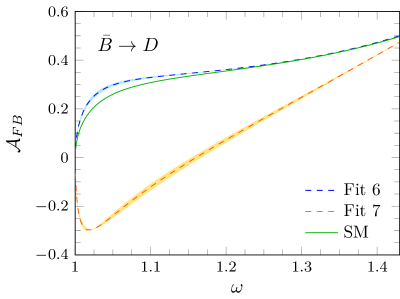
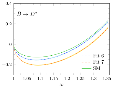
Figure 19: Forward-backward asymmetry in the CM reference frame for the $\bar{B}\to D\tau\bar{\nu}_{\tau}$ (left) and $\bar{B}\to D^{*}\tau\bar{\nu}_{\tau}$ (right) decays. Uncertainty bands as in Fig. 16.

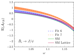
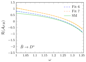
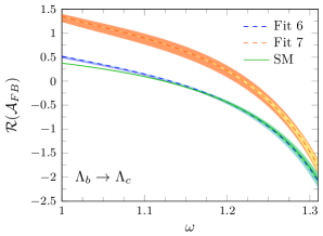
Figure 20: ${\cal R}({\cal A}_{FB})$ ratios defined in Eq. (15) for the $\bar{B}_{c}\to J/\psi$, $\bar{B}\to D^{*}$ and $\Lambda_{b}\to\Lambda_{c}$ semileptonic decays, as a function of $\omega$. Errors bands have been calculated as in Figs. 2 and 16 for the $\bar{B}_{c}$ and $\bar{B}$ meson decays. The $\Lambda_{b}$ plot has been taken from Fig.4 of Ref. Penalva et al. (2020), while for the for the $\bar{B}_{c}\to J/\psi$ decay, we also show the SM results obtained with LQCD form factors from Ref. Harrison et al. (2020a).

To minimize experimental and theoretical uncertainties, it was proposed in Ref. Penalva et al. (2020) to pay attention to the ratio ${\cal R}({\cal A_{FB}})$, defined as

$${\cal R}({\cal A}_{FB})=\frac{({\cal A}_{FB})_{\tau}}{({\cal A}_{FB})_{\ell=e,\mu}^{\rm SM}\rule{0.0pt}{8.61108pt}}=\frac{\Big{[}\frac{a_{1}\rule{0.0pt}{6.02777pt}}{2a_{0}+2a_{2}/3}\Big{]}_{\tau}\rule{0.0pt}{8.61108pt}}{\rule{0.0pt}{8.61108pt}\Big{[}\frac{a_{1}\rule{0.0pt}{6.02777pt}}{2a_{0}+2a_{2}/3}\Big{]}_{\ell=e,\mu}^{\rm SM}}$$ (15)

In Fig. 20, we show the theoretical predictions for ${\cal R}({\cal A}_{FB})$ for the $\bar{B}_{c}\to J/\psi$, $\bar{B}\to D^{*}$ and $\Lambda_{b}\to\Lambda_{c}$ semileptonic decays, with the latter taken from Ref. Penalva et al. (2020) where details of the LQCD form factors used in the calculation can be found. In addition, for $\bar{B}_{c}\to J/\psi$, we also display the SM results obtained with LQCD form factors from Ref. Harrison et al. (2020a), which agree remarkably well with the NRQM distribution. Note that for $\bar{B}_{c}\to\eta_{c}$ and $\bar{B}\to D$ decays, the denominator in Eq. (15) vanishes in the massless lepton limit ($m_{\ell}\to 0)$, since $a_{1}(\omega)=a_{1}(\omega,h=-1)+a_{1}(\omega,h=+1)$, and the negative helicity contribution is zero (Eq. (11)), while the positive helicity one is proportional to $m_{\ell}$.

The ratio ${\cal R}({\cal A}_{FB})$ can be measured by subtracting the number of events seen for $\theta_{\ell}\in[0,\pi/2]$ and for $\theta_{\ell}\in[\pi/2,\pi]$ and dividing by the total sum of observed events, in each of the $H_{b}\to H_{c}\tau\bar{\nu}_{\tau}$ and $H_{b}\to H_{c}e(\mu)\bar{\nu}_{e(\mu)}$ reactions. We expect that this observable should be free of a good part of experimental normalization errors. On the theoretical side, we see in Fig. 20 that predictions for this ratio have indeed small uncertainties, and that this quantity has the potential to establish the validity of the NP scenarios associated to Fit 7, even more if all three reactions shown in Fig. 20 are simultaneously confronted with experiment.

For completeness, $\bar{B}\to D^{(*)}$ results with a polarized final $\tau$ are given in Appendix D. Roughly, the same qualitative features that we have discussed for the polarized $\bar{B}_{c}\to\eta_{c}$ and $\bar{B}_{c}\to J/\psi$ semileptonic decays are also found in this case.

IV Conclusions

We have shown the relevant role that the $a_{0,1,2}(\omega)$ CM and $c_{0,1,2}(\omega)$ LAB scalar functions, in terms of which the CM $d^{2}\Gamma/(d\omega d\cos\theta_{\ell})$ and LAB $d^{2}\Gamma/(d\omega dE_{\ell})$ differential decay widths are expanded, could play in order to separate between different NP scenarios that otherwise give rise to the same ${\cal R}_{D^{(*)}},{\cal R}_{\eta_{c},J/\psi}$ ratios. The scheme we have used is the one originally developed in Ref. Penalva et al. (2020), and applied there to the analysis of the $\Lambda_{b}\to\Lambda_{c}\tau\bar{\nu}_{\tau}$ decay, that we have extended in this work to the study of the $\bar{B}\to D,\bar{B}\to D^{*},\bar{B}_{c}\to\eta_{c}$ and $\bar{B}_{c}\to J/\psi$ meson reactions.

For the $\bar{B}_{c}\to\eta_{c},J/\psi$ transitions we have obtained results from a NRQM scheme, consistent with the expected breaking pattern of HQSS from $\bar{B}\to D^{(*)}$ decays Neubert (1994), estimating the systematic uncertainties caused by the use of different inter-quark potentials. Besides, and since SM LQCD vector and axial form factors for $\bar{B}_{c}\to J/\psi$ have recently been reported by the HPQCD collaboration Harrison et al. (2020a), we have made systematic comparisons with the SM observables computed with the LQCD input. In general, though there appear some overall normalization inconsistencies, we find quite good agreements for $\omega-$shapes, which become much better for observables constructed out of ratios of distributions, like the $\tau-$forward-backward [${\cal A}_{FB}$] and $\tau-$polarization [${\cal A}_{\lambda_{\tau}}$] asymmetries, as well as the ratios between predictions obtained in $\tau$ and ($e/\mu$) modes like ${\cal R}_{J/\psi}$ (Table 1) or ${\cal R}({\cal A}_{FB})$ (Fig. 20). This further supports the reliability of our results for the LAB or the $\bar{B}\to\eta_{c}$ distributions, not yet studied.

As a general rule, the $\bar{B}_{c}\to J/\psi$ observables, even involving $\tau$ polarization, are less optimal for distinguishing between NP scenarios than those obtained from $\bar{B}_{c}\to\eta_{c}$ decays, or those discussed in Ref. Penalva et al. (2020) for the related $\Lambda_{b}\to\Lambda_{c}$ semileptonic decay. We have also found qualitative similar behaviors for $\bar{B}\to D$ and $\bar{B}_{c}\to\eta_{c}$, and $\bar{B}\to D^{*}$ and $\bar{B}_{c}\to J/\psi$ decay observables.

We have also drawn the attention to the ratio ${\cal R}({\cal A_{FB}})$, defined in Eq. (15) and shown in Fig. 20 for $\bar{B}_{c}\to J/\psi$, $\bar{B}\to D^{*}$ and $\Lambda_{b}\to\Lambda_{c}$ decays, as a promising quantity, both from the experimental and theoretical points of view, to shed light into details of different NP scenarios in $b\to c\tau\bar{\nu}_{\tau}$ transitions.

One should notice however that the effective Hamiltonian of Eq. (3), despite excluding right-handed neutrino terms, contains five, complex in general, NP Wilson coefficients. While one of them can always be taken to be real, that still leaves nine free parameters to be determined from data. Even assuming that the form factors were known, and therefore the genuinely hadronic part ($W$) of the $\widetilde{W}$ SFs, it would be difficult to determine all NP parameters just from the study of a unique reaction. As shown in Ref. Penalva et al. (2020), for decays with an unpolarized final $\tau$ lepton, the CM $d^{2}\Gamma/(d\omega d\cos\theta_{\ell})$ and LAB $d^{2}\Gamma/(d\omega dE_{\ell})$ differential decay widths are completely determined by only three independent functions which are linear combinations of the $\widetilde{W}$ SFs, the latter depending on the NP Wilson coefficients. This means that $a_{0,1,2}(\omega)$ and $c_{0,1,2}(\omega)$ contain the same information. For the case of polarized final $\tau$’s, the CM $d^{2}\Gamma/(d\omega d\cos\theta_{\ell})$ and LAB and $d^{2}\Gamma/(d\omega dE_{\ell})$ distributions provide complementary information giving access to another five independent linear combinations of the $\widetilde{W}$’s Penalva et al. (2020). But in this case it is the experimental measurement of the required polarized decay that could become a very difficult task. We think it is therefore more convenient to analyze data from various types of semileptonic decays simultaneously (e.g. $\bar{B}\to D,\bar{B}\to D^{*}$, $\Lambda_{b}\to\Lambda_{c},\bar{B}_{c}\to\eta_{c},\bar{B}_{c}\to J/\psi$…), considering both the $e/\mu$ and $\tau$ modes. The scheme presented in Penalva et al. (2020) is a powerful tool to achieve this objective.

Appendix A Form Factors for $P_{b}(0^{-})\to P_{c}(0^{-})$ and $P_{b}(0^{-})\to P_{c}^{*}(1^{-})$ transitions

For these two transitions we use the standard definitions of the form factors taken from Ref. Bernlochner et al. (2017),

• $P_{b}\to P_{c}$

  $$\langle P_{c};\vec{p}^{\,\prime}|\bar{c}(0)b(0)|P_{b};\vec{p}\,\rangle = \frac{1+\omega}{2}h_{S}(\omega)$$

  $$\langle P_{c};\vec{p}^{\,\prime}|\bar{c}(0)\gamma_{5}b(0)|P_{b};\vec{p}\,\rangle = \langle P_{c};\vec{p}^{\,\prime}|\bar{c}(0)\gamma^{\alpha}\gamma_{5}b(0)|P_{b};\vec{p}\,\rangle=0$$

  $$\langle P_{c};\vec{p}^{\,\prime}|\bar{c}(0)\gamma^{\alpha}b(0)|P_{b};\vec{p}\,\rangle = \frac{1}{2}\left(v^{\alpha}+v^{\prime\alpha}\right)\,h_{+}(\omega)+\frac{1}{2}\left(v^{\alpha}-v^{\prime\alpha}\right)\,h_{-}(\omega)$$

  $$\langle P_{c};\vec{p}^{\,\prime}|\bar{c}(0)\sigma^{\alpha\beta}b(0)|P_{b};\vec{p}\,\rangle = \frac{i}{2}\left(v^{\prime\alpha}v^{\beta}-v^{\prime\beta}v^{\alpha}\right)h_{T}(\omega)$$

  $$\langle P_{c};\vec{p}^{\,\prime}|\bar{c}(0)\sigma^{\alpha\beta}\gamma_{5}b(0)|P_{b};\vec{p}\,\rangle = \frac{1}{2}\epsilon^{\alpha\beta\delta\eta}v^{\prime}_{\delta}v_{\eta}h_{T}(\omega)$$ (16)

  with $v^{\alpha}=p^{\alpha}/M$ and $v^{\prime\alpha}=p^{\prime\alpha}/M^{\prime}=(p^{\alpha}-q^{\alpha})/M^{\prime}$, the quadrivelocities of the initial and final hadrons, which have masses $M$ and $M^{\prime}$, respectively, $\omega=\left(v\cdot v^{\prime}\right)$ and $\epsilon_{0123}=+1$.

• $P_{b}\to P_{c}^{*}$

  $$\langle P_{c}^{*};\vec{p}^{\,\prime},r\,|\bar{c}(0)b(0)|P_{b};\vec{p}\,\rangle = 0$$

  $$\langle P_{c}^{*};\vec{p}^{\,\prime},r\,|\bar{c}(0)\gamma_{5}b(0)|P_{b};\vec{p}\,\rangle = -\frac{1}{2}\left(\epsilon_{r}^{*}\cdot v\right)h_{P}(\omega)$$

  $$\langle P_{c}^{*};\vec{p}^{\,\prime},r\,|\bar{c}(0)\gamma^{\alpha}b(0)|P_{b};\vec{p}\,\rangle = \frac{i}{2}\epsilon^{\alpha}_{\,\,\delta\eta\gamma}\epsilon^{*\delta}_{r}v^{\prime\eta}v^{\gamma}h_{V}(\omega)$$

  $$\langle P_{c}^{*};\vec{p}^{\,\prime},r\,|\bar{c}(0)\gamma^{\alpha}\gamma_{5}b(0)|P_{b};\vec{p}\,\rangle = \frac{\omega+1}{2}\epsilon^{*\alpha}_{r}h_{A_{1}}(\omega)-\frac{\left(\epsilon^{*}_{r}\cdot v\right)}{2}\Big{[}v^{\alpha}h_{A_{2}}(\omega)+v^{\prime\alpha}h_{A_{3}}(\omega)\Big{]}$$

  $$\langle P_{c}^{*};\vec{p}^{\,\prime},r\,|\bar{c}(0)\sigma^{\alpha\beta}b(0)|P_{b};\vec{p}\,\rangle = -\frac{1}{2}\epsilon^{\alpha\beta}_{\,\,\,\,\,\,\,\delta\eta}\Big{\{}\epsilon^{*\delta}_{r}\left[\left(v^{\eta}+v^{\prime\eta}\right)\,h_{T_{1}}(\omega)+\left(v^{\eta}-v^{\prime\eta}\right)\,h_{T_{2}}(\omega)\right]+v^{\delta}v^{\prime\eta}\left(\epsilon_{r}^{*}\cdot v\right)\,h_{T_{3}}(\omega)\Big{\}}$$

  $$\langle P_{c}^{*};\vec{p}^{\,\prime},r\,|\bar{c}(0)\sigma^{\alpha\beta}\gamma_{5}b(0)|P_{b};\vec{p}\,\rangle = -\frac{i}{2}\Bigg{\{}\epsilon^{*\alpha}_{r}\left[\left(v^{\beta}+v^{\prime\beta}\right)\,h_{T_{1}}(\omega)+\left(v^{\beta}-v^{\prime\beta}\right)\,h_{T_{2}}(\omega)\right]$$ (17)

  $$-\epsilon^{*\beta}_{r}\left[\left(v^{\alpha}+v^{\prime\alpha}\right)\,h_{T_{1}}(\omega)+\left(v^{\alpha}-v^{\prime\alpha}\right)\,h_{T_{2}}(\omega)\right]$$

  $$+\left(v^{\alpha}v^{\prime\beta}-v^{\beta}v^{\prime\alpha}\right)\left(\epsilon_{r}^{*}\cdot v\right)\,h_{T_{3}}(\omega)\Bigg{\}}$$

  where $r$ is the helicity of the final vector meson, with $\epsilon_{r}$ its corresponding polarization vector. In short,

  $$\langle P_{c}^{*};\vec{p}^{\,\prime},r\,|\bar{c}(0)\Gamma^{(\alpha\beta)}b(0)|P_{b};\vec{p}\,\rangle=T^{(\alpha\beta)}_{\mu}\epsilon_{r}^{\mu*}$$ (18)

  with $\Gamma^{(\alpha\beta)}=1,\gamma_{5},\gamma^{\alpha},\gamma^{\alpha}\gamma_{5},\sigma^{\alpha\beta}$ and $\sigma^{\alpha\beta}\gamma_{5}$ and $T^{(\alpha\beta)}_{\mu}$ read from Eq. (17).

The form factors are real functions of $\omega$ greatly constrained by HQSS near zero recoil ($\omega=1$) Neubert (1994); Bernlochner et al. (2017). Indeed, all factors in Eqs. (16) and (17) have been chosen such that in the heavy quark limit each form factor either vanishes or equals the leading-order Isgur-Wise function

$$h_{-}=h_{A_{2}}=h_{T_{2}}=h_{T_{3}}=0,\quad h_{+}=h_{V}=h_{A_{1}}=h_{A_{3}}=h_{S}=h_{P}=h_{T}=h_{T_{1}}=\xi$$ (22)

The hadron tensors and $\widetilde{W}$ SFs introduced in Ref. Penalva et al. (2020) are straightforwardly obtained from Eq. (16) in the case of $P_{b}\to P_{c}$ transitions, while for decays into vector mesons, we use

$$\sum_{r}\langle P_{c}^{*};\vec{p}^{\,\prime},r\,|\bar{c}(0)\Gamma^{(\alpha\beta)}b(0)|P_{b};\vec{p}\,\rangle\langle P_{c}^{*};\vec{p}^{\,\prime},r\,|\bar{c}(0)\Gamma^{(\rho\lambda)}b(0)|P_{b};\vec{p}\,\rangle^{*}=T^{(\alpha\beta)}_{\mu}T^{(\rho\lambda)}_{\nu}\left(-g^{\mu\nu}+v^{\prime\mu}v^{\prime\nu}\right)$$ (23)

The explicit expressions for the $\widetilde{W}$ SFs in terms of the above form factors and the Wilson coefficients are given in the following appendix.

Appendix B Hadron tensor $\widetilde{W}$ SFs for the $P_{b}\to P_{c}\ell^{-}\bar{\nu}_{\ell}$ and $P_{b}\to P_{c}^{*}\ell^{-}\bar{\nu}_{\ell}$ decays

We compile here the $\widetilde{W}$ SFs introduced in Ref. Penalva et al. (2020) for the particular meson decays studied in this work. As shown in that reference, these $\widetilde{W}$ SFs determine the LAB $d^{2}\Gamma/(d\omega dE_{\ell})$ and CM $d^{2}\Gamma/(d\omega d\cos\theta_{\ell}$) differential decay widths, for the full set of NP operators in Eq. (3), for generally complex Wilson coefficients, and for the case where the final charged lepton has a well defined helicity in either reference frame. In the equations below, we use $C_{V,A}=1+C_{V_{L}}\pm C_{V_{R}}$ and $C_{S,P}=C_{S_{L}}\pm C_{S_{R}}$.

B.1 $P_{b}\to P_{c}\ell^{-}\bar{\nu}_{\ell}$

In this case, the SFs related to the SM currents are

$$\widetilde{W}_{1} = \widetilde{W}_{3}=0,\quad\widetilde{W}_{2}=\frac{|C_{V}|^{2}}{r}F_{+}^{2},\quad\widetilde{W}_{4}=\frac{|C_{V}|^{2}}{4r}(F_{+}-F_{-})^{2},\quad\widetilde{W}_{5}=\frac{|C_{V}|^{2}}{r}\,F_{+}\left(F_{-}-F_{+}\right)$$

where

$$F_{+} = \frac{1}{R}\left(h_{+}-\frac{1-r}{1+r}h_{-}\right),\quad F_{-}=\frac{1}{R}\left(h_{-}-\frac{1-r}{1+r}h_{+}\right)=\frac{1-r^{2}}{1+r^{2}-2r\omega}\left(F_{0}-F_{+}\right)$$

$$F_{0} = \frac{2r(1+\omega)}{R(1+r)^{2}}\Big{[}h_{+}-\frac{1+r}{1-r}\frac{\omega-1}{\omega+1}\,h_{-}\Big{]}$$ (25)

with $r=M^{\prime}/M$ and $R=2\sqrt{r}/(1+r)$, and we have also introduced the $F_{0}$ form-factor in the definition of $F_{-}$, as commonly done in this type of calculations. In addition,

$$\widetilde{W}_{SP} = |C_{S}|^{2}\left(\frac{1+\omega}{2}\right)^{2}h_{S}^{2},\quad\widetilde{W}_{I1}=C_{V}C_{S}^{*}\,\frac{1+\omega}{\sqrt{r}}h_{S}\,F_{+},\quad\widetilde{W}_{I2}=C_{V}C_{S}^{*}\,\frac{1+\omega}{2\sqrt{r}}h_{S}\,\left(F_{-}-F_{+}\right)$$

$$\widetilde{W}_{I3} = -C_{T}^{*}C_{S}\,\frac{1+\omega}{2r}h_{S}\,h_{T},\quad\widetilde{W}_{I4}=-C_{T}^{*}C_{V}\frac{h_{T}F_{+}}{r^{3/2}},\quad\widetilde{W}_{I5}=C_{T}^{*}C_{V}\frac{h_{T}\left(F_{+}-F-\right)}{2r^{3/2}},\quad\widetilde{W}_{I6}=\widetilde{W}_{I7}=0$$

$$\widetilde{W}_{1}^{T} = \frac{|C_{T}|^{2}}{4}\left(\omega^{2}-1\right)h_{T}^{2},\quad\widetilde{W}_{2}^{T}=\frac{|C_{T}|^{2}}{4r^{2}}\left(1+r^{2}-2r\omega\right)h_{T}^{2},\quad\widetilde{W}_{3}^{T}=\frac{|C_{T}|^{2}}{4r^{2}}h_{T}^{2},$$

$$\widetilde{W}_{4}^{T} = -\frac{|C_{T}|^{2}}{4r^{2}}\left(1-r\omega\right)h_{T}^{2},\quad\widetilde{W}_{5}^{T}=0.$$ (26)

As derived in Ref. Penalva et al. (2020), the tensor $\widetilde{W}$ SFs accomplish:

$$2\widetilde{W}_{1}^{T}+\widetilde{W}_{2}^{T}+(1-2r\omega+r^{2})\widetilde{W}_{3}^{T}+2(1-r\omega)\widetilde{W}_{4}^{T}=0$$ (27)

B.2 $P_{b}\to P_{c}^{*}\ell^{-}\bar{\nu}_{\ell}$

In this case, the $\widetilde{W}$ SFs related to the SM currents are

$$\widetilde{W}_{1} = \frac{|C_{V}|^{2}}{4}\left(\omega^{2}-1\right)h_{V}^{2}+\frac{|C_{A}|^{2}}{4}\left(\omega+1\right)^{2}h_{A_{1}}^{2}$$

$$\widetilde{W}_{2} = -\frac{|C_{V}|^{2}}{4r^{2}}\left(1+r^{2}-2r\omega\right)h_{V}^{2}+\frac{|C_{A}|^{2}}{4r^{2}}\left(\omega+1\right)^{2}\left(h_{A_{1}}^{2}-2\,\frac{\omega-r}{\omega+1}h_{A_{1}}\left(r\,h_{A_{2}}+h_{A_{3}}\right)+\frac{\omega-1}{\omega+1}\left(r\,h_{A_{2}}+h_{A_{3}}\right)^{2}\right)$$

$$\widetilde{W}_{3} = \frac{{\rm Re}[C_{V}C_{A}^{*}]}{r}(\omega+1)h_{V}h_{A_{1}}$$

$$\widetilde{W}_{4} = -\frac{|C_{V}|^{2}}{4r^{2}}h_{V}^{2}+\frac{|C_{A}|^{2}}{4r^{2}}\left(\omega+1\right)^{2}\left(h_{A_{1}}-h_{A_{3}}\right)\left(h_{A_{1}}+\frac{1-\omega}{1+\omega}\,h_{A_{3}}\right)$$

$$\widetilde{W}_{5} = \frac{|C_{V}|^{2}}{2r^{2}}\left(1-r\omega\right)h_{V}^{2}-\frac{|C_{A}|^{2}}{2r^{2}}\Big{\{}\left(1+\omega\right)\left(h_{A_{1}}-r\,h_{A_{2}}-h_{A_{3}}\right)\left[\left(1+\omega\right)h_{A_{1}}-(\omega-r)h_{A_{3}}\right]$$ (28)

$$+\left(1+\omega\right)\left(r\,h_{A_{2}}+h_{A_{3}}\right)\left(h_{A_{1}}-(1-r)h_{A_{3}}\right)\Big{\}}.$$

The rest of NP $\widetilde{W}$ SFs are

$$\widetilde{W}_{SP} = \frac{|C_{P}|^{2}}{4}\left(\omega^{2}-1\right)h_{P}^{2}$$

$$\widetilde{W}_{I1} = \frac{C_{A}C_{P}^{*}}{2r}\left(\omega^{2}-1\right)\left[r\,h_{A_{2}}+h_{A_{3}}-\frac{\omega-r}{\omega-1}\,h_{A_{1}}\right]h_{P}$$

$$\widetilde{W}_{I2} = \frac{C_{A}C_{P}^{*}}{2r}\left(\omega+1\right)\left[\omega h_{A_{1}}+\left(1-\omega\right)h_{A_{3}}\right]h_{P}$$

$$\widetilde{W}_{I3} = -\frac{C_{P}C_{T}^{*}}{2r}(\omega^{2}-1)h_{P}T_{1}$$

$$\widetilde{W}_{I4} = \frac{C_{V}C_{T}^{*}}{2r^{2}}\left[(1-r\omega)T_{2}+(\omega-r)T_{3}\right]h_{V}-\frac{C_{A}C_{T}^{*}}{2r^{2}}\Big{\{}(\omega+1)h_{A_{1}}\left[(r-\omega)T_{1}+rT_{2}+T_{3}\right]+(\omega^{2}-1)(rh_{A_{2}}+h_{A_{3}})T_{1}\Big{\}}$$

$$\widetilde{W}_{I5} = -\frac{C_{V}C_{T}^{*}}{2r^{2}}\left(T_{2}+\omega T_{3}\right)h_{V}+\frac{C_{A}C_{T}^{*}}{2r^{2}}\Big{\{}(\omega^{2}-1)h_{A_{3}}T_{1}-(\omega+1)h_{A_{1}}\left[\omega T_{1}-T_{3}\right]\Big{\}}$$

$$\widetilde{W}_{I6} = \frac{C_{V}C_{T}^{*}}{2r}(\omega^{2}-1)h_{V}\left(rT_{2}+T_{3}\right)-\frac{C_{A}C_{T}^{*}}{2r}(\omega+1)h_{A_{1}}\left[(1-r\omega)T_{2}+(\omega-r)T_{3}\right]$$

$$\widetilde{W}_{I7} = -\frac{C_{V}C_{T}^{*}}{2r}(\omega^{2}-1)h_{V}T_{3}+\frac{C_{A}C_{T}^{*}}{2r}(\omega+1)h_{A_{1}}\left[T_{2}+\omega T_{3}\right]$$

$$\widetilde{W}_{1}^{T} = \frac{|C_{T}|^{2}}{4}(\omega^{2}-1)^{2}T_{1}^{2}$$

$$\widetilde{W}_{2}^{T} = \frac{|C_{T}|^{2}}{4r^{2}}\left[(r^{2}-2r\omega+1)(\omega^{2}-1)T_{1}^{2}+(1-r^{2})(T_{3}^{2}-T_{2}^{2})+2r(1-r\omega)(\omega T_{2}+T_{3})T_{2}+2(r-\omega)(T_{2}+\omega T_{3})T_{3}\right]$$

$$\widetilde{W}_{3}^{T} = \frac{|C_{T}|^{2}}{4r^{2}}\left[(\omega^{2}-1)(T_{1}^{2}-T_{3}^{2})-(T_{2}+\omega T_{3})^{2}\right]$$

$$W_{4}^{T} = \frac{|C_{T}|^{2}}{4r^{2}}\left[(1-r\omega)(T_{2}^{2}+T_{3}^{2})+2(\omega-r)T_{2}T_{3}+(\omega^{2}-1)\left(2T_{3}^{2}-(1-r\omega)T_{1}^{2}\right)\right]$$

$$\widetilde{W}_{5}^{T} = 0$$ (29)

with the tensor $\widetilde{W}_{1,2,3,4}^{T}$ SFs satisfying Eq. (27), and

$$T_{1}=\frac{(\omega+1)h_{T_{1}}+(\omega-1)h_{T_{2}}}{\omega^{2}-1}-h_{T_{3}},\quad T_{2}=-\frac{(\omega+1)h_{T_{1}}+(\omega-1)h_{T_{2}}}{\omega^{2}-1},\quad T_{3}=\frac{(\omega+1)h_{T_{1}}-(\omega-1)h_{T_{2}}}{\omega^{2}-1}$$ (30)

Although $T_{1}$, $T_{2}$ and $T_{3}$ behave as $\pm 1/(\omega-1)$ in the heavy quark limit, the corresponding $\widetilde{W}_{1,2,3,4}^{T}$ SFs are finite at zero recoil, as they should be, with their values being given by $|C_{T}|^{2}\Big{[}1$, $-\frac{r^{2}+6r+1}{4r^{2}}$, $-\frac{1}{4r^{2}}$, $\frac{3r+1}{4r^{2}}\Big{]}$, respectively.

Appendix C Evaluation of the $\bar{B}_{c}\to\eta_{c}$ and $\bar{B}_{c}\to J/\psi$ semileptonic decay form factors within the NRQM of Ref. Hernández et al. (2006)

Within the NRQM calculation of Ref. Hernández et al. (2006), and with the global phases used in the present work, we obtain the following expressions for the different form factors.

C.1 $\bar{B}_{c}\to\eta_{c}$

For the pseudoscalar-pseudoscalar $\bar{B}_{c}\to\eta_{c}$ transition we have

$$F_{+}=\frac{1}{2M}\,\Big{(}V^{0}+{V^{3}}\frac{E^{\prime}-M}{|\vec{q}\,|}\Big{)}\ \ F_{-}=\frac{1}{2M}\,\Big{(}V^{0}+{V^{3}}\frac{E^{\prime}+M}{|\vec{q}\,|}\Big{)},$$ ,

$$h_{S}=\frac{S}{(\omega+1)\sqrt{MM^{\prime}}}\ \ h_{T}=-\sqrt{\frac{M^{\prime}}{M}}\,i\frac{T^{03}}{|\vec{q}\,|},$$ , (31)

with $F_{\pm}$ defined in Eq. (25), and where $V^{\mu}$, $S$ and $T^{\mu\nu}$ stand for the NRQM matrix elements of the vector, scalar and tensor $b\to c$ transition currents, respectively. In addition, $E^{\prime}=\sqrt{M^{\prime 2}+\vec{q}\,^{2}}$ is the energy of the final meson that has three-momentum $-\vec{q}$ in the LAB frame, with $\vec{q}$ the three-momentum transferred in the LAB frame and that for the purpose of calculation we take it along the positive $Z$ axis. For the matrix elements one has the results

$$V^{0} = \sqrt{2M2E^{\prime}}\ \int\,d^{3}p\ \frac{1}{4\pi}\big{[}\hat{\phi}^{(\eta_{c})}(|\vec{p}\,|)\big{]}^{*}\,\hat{\phi}^{(\bar{B}_{c})}\big{(}\big{|}\,\vec{p}-\frac{1}{2}\vec{q}\,\big{|}\big{)}\ \sqrt{\frac{\widehat{E}_{c}\widehat{E}_{b}}{4E_{c}E_{b}}}\left(1+\frac{(-\frac{1}{2}\,\vec{q}-\vec{p}\,)\cdot(\frac{1}{2}\,\vec{q}-\vec{p}\,)}{\widehat{E}_{c}\widehat{E}_{b}}\right),$$

$$V^{3} = \sqrt{2M2E^{\prime}}\ \int\,d^{3}p\ \frac{1}{4\pi}\big{[}\hat{\phi}^{(\eta_{c})}(|\vec{p}\,|)\big{]}^{*}\,\hat{\phi}^{(\bar{B}_{c})}\big{(}\big{|}\,\vec{p}-\frac{1}{2}\vec{q}\,\big{|}\big{)}\ \sqrt{\frac{\widehat{E}_{c}\widehat{E}_{b}}{4E_{c}E_{b}}}\left(\frac{\frac{1}{2}\,|\vec{q}\,|-p_{z}}{\widehat{E}_{b}}+\frac{-\frac{1}{2}\,|\vec{q}\,|-p_{z}}{\widehat{E}_{c}}\right),$$

$$S = \sqrt{2M2E^{\prime}}\ \int\,d^{3}p\ \frac{1}{4\pi}\big{[}\hat{\phi}^{(\eta_{c})}(|\vec{p}\,|)\big{]}^{*}\,\hat{\phi}^{(\bar{B}_{c})}\big{(}\big{|}\,\vec{p}-\frac{1}{2}\vec{q}\,\big{|}\big{)}\ \sqrt{\frac{\widehat{E}_{c}\widehat{E}_{b}}{4E_{c}E_{b}}}\left(1-\frac{(-\frac{1}{2}\,\vec{q}-\vec{p}\,)\cdot(\frac{1}{2}\,\vec{q}-\vec{p}\,)}{\widehat{E}_{c}\widehat{E}_{b}}\right),$$

$$T^{03} = i\sqrt{2M2E^{\prime}}\ \int\,d^{3}p\ \frac{1}{4\pi}\big{[}\hat{\phi}^{(\eta_{c})}(|\vec{p}\,|)\big{]}^{*}\,\hat{\phi}^{(\bar{B}_{c})}\big{(}\big{|}\,\vec{p}-\frac{1}{2}\vec{q}\,\big{|}\big{)}\ \sqrt{\frac{\widehat{E}_{c}\widehat{E}_{b}}{4E_{c}E_{b}}}\left(\frac{\frac{1}{2}\,|\vec{q}\,|-p_{z}}{\widehat{E}_{b}}-\frac{-\frac{1}{2}\,|\vec{q}\,|-p_{z}}{\widehat{E}_{c}}\right).$$ (32)

Here, $\hat{\phi}$ stands for the orbital part of the meson wave functions in momentum space and $\hat{E}_{f}=E_{f}+m_{f}$, with $m_{f},E_{f}$ the mass and relativistic energy of the quark with flavor $f$. The corresponding three-momenta are $\frac{1}{2}\,\vec{q}-\vec{p}$ for the quark $b$ and $-\frac{1}{2}\,\vec{q}-\vec{p}$ for the quark $c$.

C.2 $\bar{B}_{c}\to J/\psi$

For the pseudoscalar-vector $\bar{B}_{c}\to J/\psi$ transition we now have

$$h_{V} = \frac{M^{\prime}\sqrt{2}}{|\vec{q}\,|}\frac{V^{1}_{\lambda=-1}}{\sqrt{MM^{\prime}}},\ \ h_{P}=\frac{M^{\prime}}{|\vec{q}\,|}\frac{P_{\lambda=0}}{\sqrt{MM^{\prime}}},$$

$$h_{A_{1}} = \frac{\sqrt{2}}{\omega+1}\,\frac{A^{1}_{\lambda=-1}}{\sqrt{MM^{\prime}}},\ \ h_{A_{2}}=-\frac{M^{\prime}}{|\vec{q}\,|}\Big{[}-\frac{A^{0}_{\lambda=0}}{\sqrt{MM^{\prime}}}-\frac{E^{\prime}}{|\vec{q}\,|}\,\frac{A^{3}_{\lambda=0}}{\sqrt{MM^{\prime}}}+\sqrt{2}\,\frac{M^{\prime}}{|\vec{q}\,|}\,\frac{A^{1}_{\lambda=-1}}{\sqrt{MM^{\prime}}}\Big{]},\$$

$$h_{A_{3}} = -\frac{M^{\prime 2}}{|\vec{q}\,|^{2}}\Big{(}\frac{A^{3}_{\lambda=0}}{\sqrt{MM^{\prime}}}-\sqrt{2}\frac{E^{\prime}}{M^{\prime}}\frac{A^{1}_{\lambda=-1}}{\sqrt{MM^{\prime}}}\Big{)},$$

$$T_{1} = \frac{M^{\prime 2}}{|\vec{q}\,|^{2}}\frac{T^{12}_{\lambda=0}}{\sqrt{MM^{\prime}}},\ \ T_{2}=\sqrt{2}\,\frac{M^{\prime}}{|\vec{q}\,|}\Big{(}i\,\frac{T^{01}_{\lambda=-1}}{\sqrt{MM^{\prime}}}-\frac{E^{\prime}}{|\vec{q}\,|}\frac{T^{23}_{\lambda=-1}}{\sqrt{MM^{\prime}}}\Big{)},\ \ T_{3}=\sqrt{2}\,\frac{M^{\prime 2}}{|\vec{q}\,|^{2}}\,\frac{T^{23}_{\lambda=-1}}{\sqrt{MM^{\prime}}},$$ (33)

with $T_{1,2,3}$ defined in Eq. (30) and $V^{\mu}_{\lambda}$, $A^{\mu}_{\lambda}$, $P_{\lambda}$ and $T^{\mu\nu}_{\lambda}$ the NRQM matrix elements of the vector, axial, pseudoscalar and tensor $b\to c$ transition currents, respectively. Here, $\lambda$ is the polarization of the final $J/\psi$ meson. We use states that have well defined spin in the $Z$ direction in the $J/\psi$ rest frame. Since the $J/\psi$ three-momentum equals $-\vec{q}$ (which is directed along the negative $Z$ axis), $\lambda$ coincides with minus the helicity, the latter being the same in the CM and LAB frames. We obtain the following expressions for the matrix elements

$$V^{1}_{\lambda=-1} = \frac{-1}{\sqrt{2}}\sqrt{2M2E^{\prime}}\ \int\,d^{3}p\ \frac{1}{4\pi}\big{[}\hat{\phi}^{(J/\psi)}(|\vec{p}\,|)\big{]}^{*}\,\hat{\phi}^{(\bar{B}_{c})}\big{(}\big{|}\,\vec{p}-\frac{1}{2}\vec{q}\,\big{|}\big{)}\ \sqrt{\frac{\widehat{E}_{c}\widehat{E}_{b}}{4E_{c}E_{b}}}\left(-\frac{\frac{1}{2}\,|\vec{q}\,|-p_{z}}{\widehat{E}_{b}}+\frac{-\frac{1}{2}\,|\vec{q}\,|-p_{z}}{\widehat{E}_{c}}\right),$$

$$A^{0}_{\lambda=0} = \sqrt{2M2E^{\prime}}\ \int\,d^{3}p\ \frac{1}{4\pi}\big{[}\hat{\phi}^{(J/\psi)}(|\vec{p}\,|)\big{]}^{*}\,\hat{\phi}^{(\bar{B}_{c})}\big{(}\big{|}\,\vec{p}-\frac{1}{2}\vec{q}\,\big{|}\big{)}\ \sqrt{\frac{\widehat{E}_{c}\widehat{E}_{b}}{4E_{c}E_{b}}}\left(\frac{\frac{1}{2}\,|\vec{q}\,|-p_{z}}{\widehat{E}_{b}}+\frac{-\frac{1}{2}\,|\vec{q}\,|-p_{z}}{\widehat{E}_{c}}\right)$$

$$A^{1}_{\lambda=-1} = \frac{1}{\sqrt{2}}\sqrt{2M2E^{\prime}}\ \int\,d^{3}p\ \frac{1}{4\pi}\big{[}\hat{\phi}^{(J/\psi)}(|\vec{p}\,|)\big{]}^{*}\,\hat{\phi}^{(\bar{B}_{c})}\big{(}\big{|}\,\vec{p}-\frac{1}{2}\vec{q}\,\big{|}\big{)}\ \sqrt{\frac{\widehat{E}_{c}\widehat{E}_{b}}{4E_{c}E_{b}}}\left(1+\frac{2p_{x}^{2}-(-\frac{1}{2}\,\vec{q}-\vec{p}\,)\cdot(\frac{1}{2}\,\vec{q}-\vec{p}\,)}{\widehat{E}_{c}\widehat{E}_{b}}\right)$$

$$A^{3}_{\lambda=0} = \sqrt{2M2E^{\prime}}\ \int\,d^{3}p\ \frac{1}{4\pi}\big{[}\hat{\phi}^{(J/\psi)}(|\vec{p}\,|)\big{]}^{*}\,\hat{\phi}^{(\bar{B}_{c})}\big{(}\big{|}\,\vec{p}-\frac{1}{2}\vec{q}\,\big{|}\big{)}\ \sqrt{\frac{\widehat{E}_{c}\widehat{E}_{b}}{4E_{c}E_{b}}}\ \left(1+\frac{2(-\frac{1}{2}\,|\vec{q}\,|-p_{z}\,)\,(\frac{1}{2}\,|\vec{q}\,|-p_{z}\,)}{\widehat{E}_{c}\widehat{E}_{b}}\right.$$

$$\left.-\frac{(-\frac{1}{2}\,\vec{q}-\vec{p}\,)\cdot(\frac{1}{2}\,\vec{q}-\vec{p}\,)}{\widehat{E}_{c}\widehat{E}_{b}}\right),$$

$$P_{\lambda=0} = \sqrt{2M2E^{\prime}}\ \int\,d^{3}p\ \frac{1}{4\pi}\big{[}\hat{\phi}^{(J/\psi)}(|\vec{p}\,|)\big{]}^{*}\,\hat{\phi}^{(\bar{B}_{c})}\big{(}\big{|}\,\vec{p}-\frac{1}{2}\vec{q}\,\big{|}\big{)}\ \sqrt{\frac{\widehat{E}_{c}\widehat{E}_{b}}{4E_{c}E_{b}}}\left(\frac{\frac{1}{2}\,|\vec{q}\,|-p_{z}}{\widehat{E}_{b}}-\frac{-\frac{1}{2}\,|\vec{q}\,|-p_{z}}{\widehat{E}_{c}}\right)$$

$$T^{12}_{\lambda=0} = \sqrt{2M2E^{\prime}}\ \int\,d^{3}p\ \frac{1}{4\pi}\big{[}\hat{\phi}^{(J/\psi)}(|\vec{p}\,|)\big{]}^{*}\,\hat{\phi}^{(\bar{B}_{c})}\big{(}\big{|}\,\vec{p}-\frac{1}{2}\vec{q}\,\big{|}\big{)}\ \sqrt{\frac{\widehat{E}_{c}\widehat{E}_{b}}{4E_{c}E_{b}}}\ \left(1-\frac{2(-\frac{1}{2}\,|\vec{q}\,|-p_{z}\,)\,(\frac{1}{2}\,|\vec{q}\,|-p_{z}\,)}{\widehat{E}_{c}\widehat{E}_{b}}\right.$$

$$\left.+\frac{(-\frac{1}{2}\,\vec{q}-\vec{p}\,)\cdot(\frac{1}{2}\,\vec{q}-\vec{p}\,)}{\widehat{E}_{c}\widehat{E}_{b}}\right),$$

$$T^{23}_{\lambda=-1} = \frac{1}{\sqrt{2}}\sqrt{2M2E^{\prime}}\ \int\,d^{3}p\ \frac{1}{4\pi}\big{[}\hat{\phi}^{(J/\psi)}(|\vec{p}\,|)\big{]}^{*}\,\hat{\phi}^{(\bar{B}_{c})}\big{(}\big{|}\,\vec{p}-\frac{1}{2}\vec{q}\,\big{|}\big{)}\ \sqrt{\frac{\widehat{E}_{c}\widehat{E}_{b}}{4E_{c}E_{b}}}\left(1-\frac{2p_{x}^{2}-(-\frac{1}{2}\,\vec{q}-\vec{p}\,)\cdot(\frac{1}{2}\,\vec{q}\,-\vec{p}\,)}{\widehat{E}_{c}\widehat{E}_{b}}\right),$$

$$T^{01}_{\lambda=-1} = \frac{-i}{\sqrt{2}}\sqrt{2M2E^{\prime}}\ \int\,d^{3}p\ \frac{1}{4\pi}\big{[}\hat{\phi}^{(J/\psi)}(|\vec{p}\,|)\big{]}^{*}\,\hat{\phi}^{(\bar{B}_{c})}\big{(}\big{|}\,\vec{p}-\frac{1}{2}\vec{q}\,\big{|}\big{)}\ \sqrt{\frac{\widehat{E}_{c}\widehat{E}_{b}}{4E_{c}E_{b}}}\left(-\frac{\frac{1}{2}\,|\vec{q}\,|-p_{z}}{\widehat{E}_{b}}-\frac{-\frac{1}{2}\,|\vec{q}\,|-p_{z}}{\widehat{E}_{c}}\right).$$

Appendix D Results for the $\bar{B}\to D\tau\bar{\nu}_{\tau}$ and $\bar{B}\to D^{*}\tau\bar{\nu}_{\tau}$ decays for the case of a polarized final $\tau$

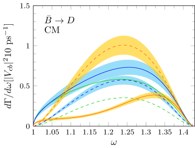
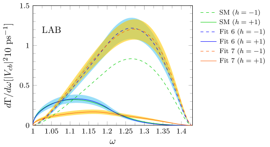
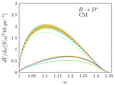
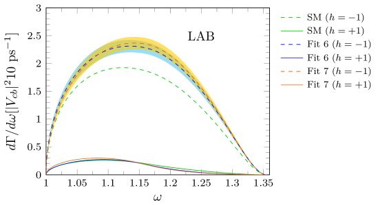
Figure 21: CM (left) and LAB (right) helicity decomposition of the $d\Gamma/d\omega$ differential decay width with a polarized $\tau$. We show distributions for $\bar{B}\to D\tau\bar{\nu}_{\tau}$ (top) and $\bar{B}\to D^{*}\tau\bar{\nu}_{\tau}$ reactions (bottom), which have been evaluated with Wilson coefficients and form factors from Ref. Murgui et al. (2019). Uncertainty bands as in Fig. 16.

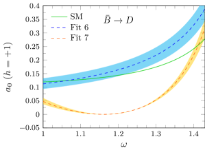
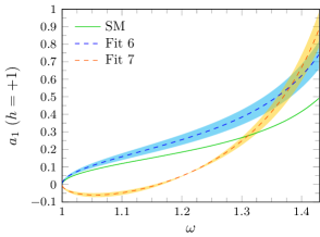
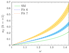
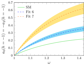
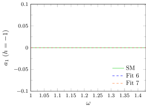
Figure 22: CM angular expansion coefficients for the $\bar{B}\to D\tau\bar{\nu}_{\tau}$ decay with a polarized $\tau$ with positive (upper panels) and negative (lower panels) helicity. They have been evaluated with the Wilson coefficients and form factors from Ref. Murgui et al. (2019). Uncertainty bands as in Fig. 16.

In this appendix we collect in Figs. 21–26, results for $\bar{B}\to D\tau\bar{\nu}_{\tau}$ and $\bar{B}\to D^{*}\tau\bar{\nu}_{\tau}$ decays where the final $\tau$ has well defined helicity in the CM or LAB frames. All observables have been evaluated with the NP Wilson coefficients of Fits 6 and 7 and form factors from Ref. Murgui et al. (2019).

We obtain predictions that are qualitatively similar to those discussed in Sec. II for $\bar{B}_{c}\to\eta_{c}$ and $\bar{B}_{c}\to J/\psi$ semileptonic decays. We would like to stress that unlike the unpolarized case, where all the accessible observables could be determined either from the CM or LAB distributions, in the polarized case, the LAB and CM charged lepton helicity distributions provide complementary information. Actually both differential distributions $d^{2}\Gamma/(d\omega d\cos\theta_{\ell})$ and $d^{2}\Gamma/(d\omega dE_{\ell})$ should be simultaneously used to determine the five new independent functions ${\cal A}_{H},{\cal B}_{H},{\cal C}_{H},{\cal D}_{H}$ and ${\cal E}_{H}$, which appear for the case of a polarized final $\tau$ (see Eq. (23) of Ref. Penalva et al. (2020)).

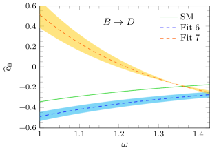
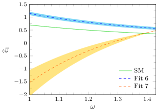
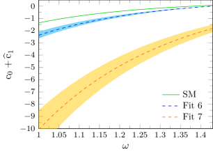
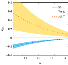
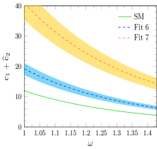
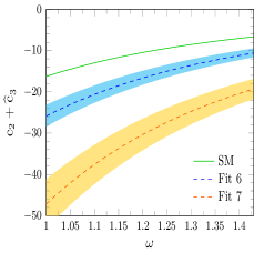
Figure 23: LAB charged lepton energy expansion coefficients $\widehat{c}_{0,1,2,3}(\omega)$ for the polarized $\bar{B}\to D\tau\bar{\nu}_{\tau}$ decay. We also show the $(c_{0}+\widehat{c}_{1})$, $(c_{1}+\widehat{c}_{2})$ and $(c_{2}+\widehat{c}_{3})$ sums in the third top, second and fourth bottom panels, respectively. All quantities have been evaluated with the Wilson coefficients and form factors from Ref. Murgui et al. (2019). Uncertainty bands as in Fig. 16.

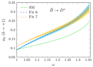
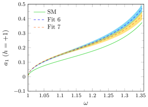
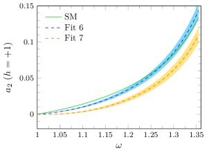
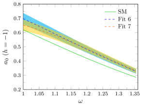
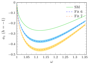
Figure 24: CM angular expansion coefficients for the $\bar{B}\to D^{*}\tau\bar{\nu}_{\tau}$ decay with a $\tau$ with positive (upper panels) and negative (lower panels) helicity. They have been evaluated with the Wilson coefficients and form factors from Ref. Murgui et al. (2019). Uncertainty bands as in Fig. 16.

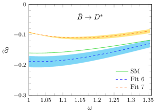
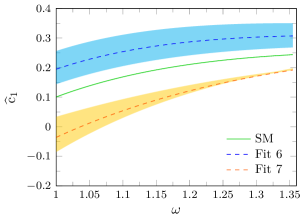
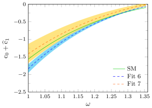
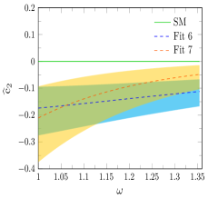
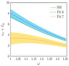
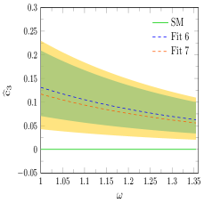
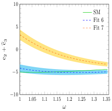
Figure 25: LAB charged lepton energy expansion coefficients $\widehat{c}_{0,1,2,3}(\omega)$ for the polarized $\bar{B}\to D^{*}\tau\bar{\nu}_{\tau}$ decay. We also show the $(c_{0}+\widehat{c}_{1})$, $(c_{1}+\widehat{c}_{2})$ and $(c_{2}+\widehat{c}_{3})$ sums in the third top, second and fourth bottom panels, respectively. All quantities have been evaluated with the Wilson coefficients and form factors from Ref. Murgui et al. (2019). Uncertainty bands as in Fig. 16.

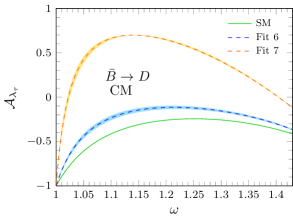
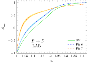
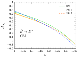
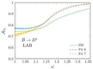
Figure 26: $\tau$ polarization asymmetry ${\cal A}_{\lambda_{\tau}}$ for the $\bar{B}\to D$ (upper panels) and $\bar{B}\to D^{*}$ (lower panels) semileptonic decays measured in the CM (left panels) and LAB (right panels) frames. All quantities have been evaluated with the Wilson coefficients and form factors from Ref. Murgui et al. (2019). Uncertainty bands as in Fig. 16.

References

- Amhis et al. (2019) Y. S. Amhis et al. (HFLAV), (2019), arXiv:1909.12524 [hep-ex] .
- Amhis et al. (2017) Y. Amhis et al. (HFLAV), Eur. Phys. J. C77, 895 (2017), online update at https://hflav.web.cern.ch/, arXiv:1612.07233 [hep-ex] .
- Lees et al. (2012) J. P. Lees et al. (BaBar), Phys. Rev. Lett. 109, 101802 (2012), arXiv:1205.5442 [hep-ex] .
- Lees et al. (2013) J. P. Lees et al. (BaBar), Phys. Rev. D88, 072012 (2013), arXiv:1303.0571 [hep-ex] .
- Huschle et al. (2015) M. Huschle et al. (Belle), Phys. Rev. D92, 072014 (2015), arXiv:1507.03233 [hep-ex] .
- Sato et al. (2016) Y. Sato et al. (Belle), Phys. Rev. D94, 072007 (2016), arXiv:1607.07923 [hep-ex] .
- Hirose et al. (2017) S. Hirose et al. (Belle), Phys. Rev. Lett. 118, 211801 (2017), arXiv:1612.00529 [hep-ex] .
- Caria et al. (2020) G. Caria et al. (Belle), Phys. Rev. Lett. 124, 161803 (2020), arXiv:1910.05864 [hep-ex] .
- Aaij et al. (2015) R. Aaij et al. (LHCb), Phys. Rev. Lett. 115, 111803 (2015), [Erratum: Phys. Rev. Lett.115,no.15,159901(2015)], arXiv:1506.08614 [hep-ex] .
- Aaij et al. (2018a) R. Aaij et al. (LHCb), Phys. Rev. Lett. 120, 171802 (2018a), arXiv:1708.08856 [hep-ex] .
- Aoki et al. (2017) S. Aoki et al., Eur. Phys. J. C77, 112 (2017), arXiv:1607.00299 [hep-lat] .
- Bigi and Gambino (2016) D. Bigi and P. Gambino, Phys. Rev. D94, 094008 (2016), arXiv:1606.08030 [hep-ph] .
- Bigi et al. (2017) D. Bigi, P. Gambino, and S. Schacht, JHEP 11, 061 (2017), arXiv:1707.09509 [hep-ph] .
- Jaiswal et al. (2017) S. Jaiswal, S. Nandi, and S. K. Patra, JHEP 12, 060 (2017), arXiv:1707.09977 [hep-ph] .
- Bernlochner et al. (2017) F. U. Bernlochner, Z. Ligeti, M. Papucci, and D. J. Robinson, Phys. Rev. D95, 115008 (2017), [erratum: Phys. Rev.D97,no.5,059902(2018)], arXiv:1703.05330 [hep-ph] .
- Aaij et al. (2018b) R. Aaij et al. (LHCb), Phys. Rev. Lett. 120, 121801 (2018b), arXiv:1711.05623 [hep-ex] .
- Anisimov et al. (1999) A. Yu. Anisimov, I. M. Narodetsky, C. Semay, and B. Silvestre-Brac, Phys. Lett. B452, 129 (1999), arXiv:hep-ph/9812514 [hep-ph] .
- Ivanov et al. (2006) M. A. Ivanov, J. G. Korner, and P. Santorelli, Phys. Rev. D73, 054024 (2006), arXiv:hep-ph/0602050 [hep-ph] .
- Hernández et al. (2006) E. Hernández, J. Nieves, and J. Verde-Velasco, Phys. Rev. D 74, 074008 (2006), arXiv:hep-ph/0607150 .
- Huang and Zuo (2007) T. Huang and F. Zuo, Eur. Phys. J. C51, 833 (2007), arXiv:hep-ph/0702147 [HEP-PH] .
- Wang et al. (2009) W. Wang, Y.-L. Shen, and C.-D. Lu, Phys. Rev. D79, 054012 (2009), arXiv:0811.3748 [hep-ph] .
- Wang et al. (2013) W.-F. Wang, Y.-Y. Fan, and Z.-J. Xiao, Chin. Phys. C37, 093102 (2013), arXiv:1212.5903 [hep-ph] .
- Watanabe (2018) R. Watanabe, Phys. Lett. B 776, 5 (2018), arXiv:1709.08644 [hep-ph] .
- Issadykov and Ivanov (2018) A. Issadykov and M. A. Ivanov, Phys. Lett. B783, 178 (2018), arXiv:1804.00472 [hep-ph] .
- Tran et al. (2018) C.-T. Tran, M. A. Ivanov, J. G. Körner, and P. Santorelli, Phys. Rev. D97, 054014 (2018), arXiv:1801.06927 [hep-ph] .
- Hu et al. (2020) X.-Q. Hu, S.-P. Jin, and Z.-J. Xiao, Chin. Phys. C44, 023104 (2020), arXiv:1904.07530 [hep-ph] .
- Leljak et al. (2019) D. Leljak, B. Melic, and M. Patra, JHEP 05, 094 (2019), arXiv:1901.08368 [hep-ph] .
- Azizi et al. (2019) K. Azizi, Y. Sarac, and H. Sundu, Phys. Rev. D99, 113004 (2019), arXiv:1904.08267 [hep-ph] .
- Wang and Zhu (2019) W. Wang and R. Zhu, Int. J. Mod. Phys. A 34, 1950195 (2019), arXiv:1808.10830 [hep-ph] .
- Fajfer et al. (2012) S. Fajfer, J. F. Kamenik, and I. Nisandzic, Phys. Rev. D85, 094025 (2012), arXiv:1203.2654 [hep-ph] .
- Murgui et al. (2019) C. Murgui, A. Peñuelas, M. Jung, and A. Pich, JHEP 09, 103 (2019), arXiv:1904.09311 [hep-ph] .
- Penalva et al. (2019) N. Penalva, E. Hernández, and J. Nieves, Phys. Rev. D100, 113007 (2019), arXiv:1908.02328 [hep-ph] .
- Penalva et al. (2020) N. Penalva, E. Hernández, and J. Nieves, Phys. Rev. D 101, 113004 (2020), arXiv:2004.08253 [hep-ph] .
- Aaij et al. (2017) R. Aaij et al. (LHCb), Phys. Rev. D96, 112005 (2017), arXiv:1709.01920 [hep-ex] .
- Cerri et al. (2019) A. Cerri et al., “Report from Working Group 4: Opportunities in Flavour Physics at the HL-LHC and HE-LHC,” in Report on the Physics at the HL-LHC,and Perspectives for the HE-LHC, Vol. 7, edited by A. Dainese, M. Mangano, A. B. Meyer, A. Nisati, G. Salam, and M. A. Vesterinen (2019) pp. 867–1158, arXiv:1812.07638 [hep-ph] .
- Bailey et al. (2014) J. A. Bailey et al. (Fermilab Lattice, MILC), Phys. Rev. D 89, 114504 (2014), arXiv:1403.0635 [hep-lat] .
- Bailey et al. (2015) J. A. Bailey et al. (Fermilab Lattice and MILC), Phys. Rev. D92, 034506 (2015), arXiv:1503.07237 [hep-lat] .
- Na et al. (2015) H. Na, C. M. Bouchard, G. P. Lepage, C. Monahan, and J. Shigemitsu (HPQCD), Phys. Rev. D92, 054510 (2015), [Erratum: Phys. Rev.D93,no.11,119906(2016)], arXiv:1505.03925 [hep-lat] .
- Harrison et al. (2018) J. Harrison, C. Davies, and M. Wingate (HPQCD), Phys. Rev. D 97, 054502 (2018), arXiv:1711.11013 [hep-lat] .
- Faller et al. (2009) S. Faller, A. Khodjamirian, C. Klein, and T. Mannel, Eur. Phys. J. C 60, 603 (2009), arXiv:0809.0222 [hep-ph] .
- Neubert et al. (1993a) M. Neubert, Z. Ligeti, and Y. Nir, Phys. Lett. B 301, 101 (1993a), arXiv:hep-ph/9209271 .
- Neubert et al. (1993b) M. Neubert, Z. Ligeti, and Y. Nir, Phys. Rev. D 47, 5060 (1993b), arXiv:hep-ph/9212266 .
- Ligeti et al. (1994) Z. Ligeti, Y. Nir, and M. Neubert, Phys. Rev. D 49, 1302 (1994), arXiv:hep-ph/9305304 .
- Datta et al. (2012) A. Datta, M. Duraisamy, and D. Ghosh, Phys. Rev. D 86, 034027 (2012), arXiv:1206.3760 [hep-ph] .
- Duraisamy and Datta (2013) M. Duraisamy and A. Datta, JHEP 09, 059 (2013), arXiv:1302.7031 [hep-ph] .
- Duraisamy et al. (2014) M. Duraisamy, P. Sharma, and A. Datta, Phys. Rev. D 90, 074013 (2014), arXiv:1405.3719 [hep-ph] .
- Ligeti et al. (2017) Z. Ligeti, M. Papucci, and D. J. Robinson, JHEP 01, 083 (2017), arXiv:1610.02045 [hep-ph] .
- Becirevic et al. (2019) D. Becirevic, S. Fajfer, I. Nisandzic, and A. Tayduganov, Nucl. Phys. B 946, 114707 (2019), arXiv:1602.03030 [hep-ph] .
- Bhattacharya et al. (2019) S. Bhattacharya, S. Nandi, and S. Kumar Patra, Eur. Phys. J. C 79, 268 (2019), arXiv:1805.08222 [hep-ph] .
- Blanke et al. (2019a) M. Blanke, A. Crivellin, S. de Boer, T. Kitahara, M. Moscati, U. Nierste, and I. Nišandžić, Phys. Rev. D99, 075006 (2019a), arXiv:1811.09603 [hep-ph] .
- Blanke et al. (2019b) M. Blanke, A. Crivellin, T. Kitahara, M. Moscati, U. Nierste, and I. Nišandžić, Phys. Rev. D100, 035035 (2019b), arXiv:1905.08253 [hep-ph] .
- Alok et al. (2020) A. K. Alok, D. Kumar, S. Kumbhakar, and S. Uma Sankar, Nucl. Phys. B 953, 114957 (2020), arXiv:1903.10486 [hep-ph] .
- Jaiswal et al. (2020) S. Jaiswal, S. Nandi, and S. K. Patra, JHEP 06, 165 (2020), arXiv:2002.05726 [hep-ph] .
- Iguro and Watanabe (2020) S. Iguro and R. Watanabe, JHEP 08, 006 (2020), arXiv:2004.10208 [hep-ph] .
- Kumbhakar (2020) S. Kumbhakar, (2020), arXiv:2007.08132 [hep-ph] .
- Bhattacharya et al. (2020) B. Bhattacharya, A. Datta, S. Kamali, and D. London, JHEP 07, 194 (2020), arXiv:2005.03032 [hep-ph] .
- Dutta and Bhol (2017) R. Dutta and A. Bhol, Phys. Rev. D 96, 076001 (2017), arXiv:1701.08598 [hep-ph] .
- Kiselev et al. (2000) V. Kiselev, A. Likhoded, and A. Onishchenko, Nucl. Phys. B 569, 473 (2000), arXiv:hep-ph/9905359 .
- Kiselev (2002) V. Kiselev, (2002), arXiv:hep-ph/0211021 .
- Cohen et al. (2019) T. D. Cohen, H. Lamm, and R. F. Lebed, Phys. Rev. D 100, 094503 (2019), arXiv:1909.10691 [hep-ph] .
- Colquhoun et al. (2016) B. Colquhoun, C. Davies, J. Koponen, A. Lytle, and C. McNeile (HPQCD), PoS LATTICE2016, 281 (2016), arXiv:1611.01987 [hep-lat] .
- Harrison et al. (2020a) J. Harrison, C. T. Davies, and A. Lytle, (2020a), arXiv:2007.06957 [hep-lat] .
- Harrison et al. (2020b) J. Harrison, C. T. Davies, and A. Lytle (LATTICE-HPQCD), (2020b), arXiv:2007.06956 [hep-lat] .
- Semay and Silvestre-Brac (1994) C. Semay and B. Silvestre-Brac, Z. Phys. C 61, 271 (1994).
- Silvestre-Brac (1996) B. Silvestre-Brac, Few Body Syst. 20, 1 (1996).
- Bhaduri et al. (1981) R. Bhaduri, L. Cohler, and Y. Nogami, Nuovo Cim. A 65, 376 (1981).
- Sakaki et al. (2015) Y. Sakaki, M. Tanaka, A. Tayduganov, and R. Watanabe, Phys. Rev. D 91, 114028 (2015), arXiv:1412.3761 [hep-ph] .
- Asadi et al. (2018) P. Asadi, M. R. Buckley, and D. Shih, JHEP 09, 010 (2018), arXiv:1804.04135 [hep-ph] .
- Greljo et al. (2018) A. Greljo, D. J. Robinson, B. Shakya, and J. Zupan, JHEP 09, 169 (2018), arXiv:1804.04642 [hep-ph] .
- Robinson et al. (2019) D. J. Robinson, B. Shakya, and J. Zupan, JHEP 02, 119 (2019), arXiv:1807.04753 [hep-ph] .
- Azatov et al. (2018) A. Azatov, D. Barducci, D. Ghosh, D. Marzocca, and L. Ubaldi, JHEP 10, 092 (2018), arXiv:1807.10745 [hep-ph] .
- Heeck and Teresi (2018) J. Heeck and D. Teresi, JHEP 12, 103 (2018), arXiv:1808.07492 [hep-ph] .
- Asadi et al. (2019) P. Asadi, M. R. Buckley, and D. Shih, Phys. Rev. D 99, 035015 (2019), arXiv:1810.06597 [hep-ph] .
- Babu et al. (2019) K. Babu, B. Dutta, and R. N. Mohapatra, JHEP 01, 168 (2019), arXiv:1811.04496 [hep-ph] .
- Bardhan and Ghosh (2019) D. Bardhan and D. Ghosh, Phys. Rev. D 100, 011701 (2019), arXiv:1904.10432 [hep-ph] .
- Shi et al. (2019) R.-X. Shi, L.-S. Geng, B. Grinstein, S. Jäger, and J. Martin Camalich, JHEP 12, 065 (2019), arXiv:1905.08498 [hep-ph] .
- Gómez et al. (2019) J. D. Gómez, N. Quintero, and E. Rojas, Phys. Rev. D 100, 093003 (2019), arXiv:1907.08357 [hep-ph] .
- Mandal et al. (2020) R. Mandal, C. Murgui, A. Peñuelas, and A. Pich, JHEP 08, 022 (2020), arXiv:2004.06726 [hep-ph] .
- Aubert et al. (2009) B. Aubert et al. (BaBar), Phys. Rev. D 79, 012002 (2009), arXiv:0809.0828 [hep-ex] .
- Neubert (1994) M. Neubert, Phys. Rept. 245, 259 (1994), arXiv:hep-ph/9306320 [hep-ph] .
- Jenkins et al. (1993) E. E. Jenkins, M. E. Luke, A. V. Manohar, and M. J. Savage, Nucl. Phys. B 390, 463 (1993), arXiv:hep-ph/9204238 .