NLO QCD corrections to off-shell $\text{t}\overline{\text{t}}\text{W}^{+}$ production at the LHC

Abstract

We present results of a computation of NLO QCD corrections to the production of an off-shell top–antitop pair in association with an off-shell $\text{W}^{+}$ boson in proton–proton collisions. As the calculation is based on the full matrix elements for the process $\text{p}\text{p}\to{\text{e}}^{+}\nu_{\text{e}}\,\mu^{-}\overline{\nu}_{\mu}\,\tau^{+}\nu_{\tau}\,{\text{b}}\,\overline{\text{b}}$, all off-shell, spin-correlation, and interference effects are included. The NLO QCD corrections are about $20\%$ for the integrated cross-section. Using a dynamical scale, the corrections to most distributions are at the same level, while some distributions show much larger $K$-factors in suppressed regions of phase space. We have performed a second calculation based on a double-pole approximation. While the corresponding results agree with the full calculation within few per cent for integrated cross-sections, the discrepancy can reach $10\%$ and more in regions of phase space that are not dominated by top–antitop production. As a consequence, on-shell calculations should only be trusted to this level of accuracy.

1 Introduction

The production of top–antitop-quark pairs in association with a massive electroweak vector boson is of great importance at the Large Hadron Collider (LHC), both as a test of the Standard Model (SM) and for the search for effects of new physics. The presence of a dominant resonance structure that features three massive unstable particles makes such a process one of the heaviest signatures that can be detected and investigated at the LHC.

Both $\text{t}\overline{\text{t}}\text{W}^{\pm}$ and $\text{t}\overline{\text{t}}\text{Z}$ production have been observed and studied by the ATLAS and CMS experiments with $8\,\text{TeV}$ Aad:2015eua ; Khachatryan:2015sha and $13\,\text{TeV}$ centre-of-mass (CM) energy data Aaboud:2016xve ; Sirunyan:2017uzs ; Aaboud:2019njj ; CMS:2019too . In particular, the ATLAS collaboration has measured ${\text{t}\overline{\text{t}}}\text{W}^{\pm}$ production in the three-charged-leptons channel Aaboud:2019njj , which is the process considered in this paper. The collected data of the LHC Runs 1 and 2 and the luminosities expected in the coming runs will deliver an improved understanding of the dynamics of $\text{t}\overline{\text{t}}V$ processes.

The study of $\text{t}\overline{\text{t}}V$ production is expected to provide a direct access to the top-quark coupling to gauge bosons, and specifically to possible deviations from the SM prediction due to new physics Dror:2015nkp ; Buckley:2015lku ; Bylund:2016phk . The $\text{t}\overline{\text{t}}\text{W}^{\pm}$ and $\text{t}\overline{\text{t}}\text{Z}$ signatures can be directly affected by beyond-Standard Model (BSM) effects, for example by the presence of supersymmetry Guchait:1994zk ; Barnett:1993ea , vector-like quarks Aguilar-Saavedra:2013qpa , little Higgs bosons Perelstein:2005ka and technicolour Chivukula:1994mn . The SM $\text{t}\overline{\text{t}}\text{Z}$ production, with $\text{Z}\rightarrow\nu\overline{\nu}$, represents an important background for dark-matter signals Bevilacqua:2019cvp .

In particular, the associated production of top quarks with a $\text{W}^{\pm}$ boson in the fully-leptonic decay channel represents a rare process at the LHC, owing to the presence of two like-sign leptons in the final state. Therefore, despite a relatively low rate, it constitutes an optimal signature for BSM searches, with a particular focus on supersymmetry Barnett:1993ea ; Guchait:1994zk , supergravity Baer:1995va , Majorana neutrinos Almeida:1997em and modified Higgs sectors Maalampi:2002vx ; Contino:2008hi . The $\text{t}\overline{\text{t}}\text{W}^{\pm}$ signature could noticeably improve the investigation of the $\text{t}\overline{\text{t}}$ charge asymmetry Maltoni:2014zpa , that is expected to be larger than in pure $\text{t}\overline{\text{t}}$ production, due to the absence of neutral initial states at leading order (LO) and next-to-leading order (NLO). Moreover, the study of polarisation-related observables in $\text{t}\overline{\text{t}}\text{W}^{\pm}$ production provides additional sensitivity to BSM effects Maltoni:2014zpa .

The $\text{t}\overline{\text{t}}V$ production is also an important background for top–antitop production in association with a Higgs boson Maltoni:2015ena , which has been recently observed Aaboud:2018urx ; Sirunyan:2018hoz and further investigated in the multi-lepton channel ATLAS-CONF-2019-045 ; CMS-PAS-HIG-17-004 at the LHC.

Both in the direct measurement of $\text{t}\overline{\text{t}}\text{W}^{\pm}$ production Sirunyan:2017uzs ; Aaboud:2019njj and in the measurement of the $\text{t}\overline{\text{t}}\text{H}$ signal ATLAS-CONF-2019-045 ; CMS-PAS-HIG-17-004 , a tension between $13\,\text{TeV}$ CM data and the SM predictions has been observed in the $\text{t}\overline{\text{t}}\text{W}^{\pm}$ modelling, both in the inclusive cross-section, and in kinematic regimes where $\text{t}\overline{\text{t}}\text{W}^{\pm}$ production is expected to be the leading contribution. In order to address such a tension with the data and to allow for more precise investigations, improved precision and accuracy are needed for the theoretical description of this process.

A number of phenomenological studies are already present in the literature. The hadronic production of $\text{t}\overline{\text{t}}\text{W}^{\pm}$ was first computed with NLO QCD accuracy for LHC energies including top-quark decays with full spin correlations, using decay chains to simulate the semileptonic final state Campbell:2012dh . Parton-shower effects of both $\text{t}\overline{\text{t}}\text{W}^{\pm}$ and $\text{t}\overline{\text{t}}\text{Z}$ production with semileptonic top decays were added on top of NLO QCD predictions for the two- (W) and three-charged-leptons (Z) final states at the LHC at $7/8\,\text{TeV}$ CM energy Garzelli:2012bn . The importance of this processes for the study of the $\text{t}\overline{\text{t}}$ charge asymmetry Maltoni:2014zpa and its impact on $\text{t}\overline{\text{t}}\text{H}$ searches Maltoni:2015ena was examined at NLO QCD in inclusive production. The impact of electroweak corrections on $\text{t}\overline{\text{t}}\text{W}^{\pm}$ production was investigated in inclusive production (no decays of the three resonances) in Refs. Frixione:2015zaa ; Frederix:2017wme . Resummed calculations for the on-shell production of $\text{t}\overline{\text{t}}$ in association with a heavy boson were performed up to next-to-next-to-leading-logarithmic (NNLL) accuracy Li:2014ula ; Broggio:2016zgg ; Kulesza:2018tqz ; Broggio:2019ewu ; Kulesza:2020nfh . An NLO QCD analysis including parton-shower matching with the focus of effects of spin correlations and subleading electroweak corrections on asymmetries was presented in Ref. Frederix:2020jzp . The first computation of NLO QCD corrections including all off-shell effects and spin correlations appeared very recently Bevilacqua:2020pzy for hadronic collisions at $13\,\text{TeV}$ CM energy in the three-charged-leptons decay channel.

The goal of this paper is to present an independent computation of the complete NLO QCD corrections to the off-shell production of $\text{t}\overline{\text{t}}\text{W}^{+}$ in the three-charged-leptons decay channel. The specific final state we consider, the scale choices we analyse, and the SM input parameters differ from those of Ref. Bevilacqua:2020pzy . However, we have reproduced the results of Ref. Bevilacqua:2020pzy using the same setup employed therein, finding very good agreement both at the integrated and at the differential level.

This work is organised as follows. In Section 2 we present details of our calculation of the ${\text{t}\overline{\text{t}}\text{W}^{+}}$ process, including a description of real and virtual NLO corrections. We describe an approximated calculation of the same process that relies on double-pole-approximation techniques and a number of numerical checks we have performed to validate the full off-shell computation. In Section 3 we present the results of numerical simulations both at the integrated and at the differential level. After introducing the setup for the numerical simulations in Section 3.1, we discuss the scale choice in Sections 3.2 and 3.3.1. In Section 3.3.2 we analyse a number of kinematic variables, including both directly measurable observables at the LHC and kinematic variables based on Monte Carlo truth. The results obtained from full matrix elements are compared with those in the double-pole approximation in Section 3.4. We draw our conclusions in Section 4.

2 Details of the calculation

In this paper we present the NLO QCD corrections to the process

$$\text{p}\text{p}\to{\text{e}}^{+}\nu_{\text{e}}\,\mu^{-}\overline{\nu}_{\mu}\,\tau^{+}\nu_{\tau}\,{\text{b}}\,\overline{\text{b}}\,.$$ (1)

The calculation has been performed with MoCaNLO, a Monte Carlo generator that has been used to simulate other processes involving top quarks with NLO EW and QCD accuracy Denner:2015yca ; Denner:2016jyo ; Denner:2017kzu ; Denner:2016wet . It is interfaced with Recola Actis:2012qn ; Actis:2016mpe which provides the tree-level and one-loop SM amplitudes using the Collier library Denner:2016kdg to perform the reduction and numerical evaluation of one-loop integrals Denner:2002ii ; Denner:2005nn ; Denner:2010tr .

The leading tree-level contributions to the considered process are of order ${\cal O}(\alpha_{\text{s}}^{2}\alpha^{6})$, and come uniquely from quark-induced partonic channels. Since we assume a diagonal quark-mixing matrix, the only possible initial states are ${\text{u}}\bar{\text{d}}$ and ${\text{c}}\bar{\text{s}}$. Similarly to $\text{t}\overline{\text{t}}$ production, other LO contributions are either suppressed [${\cal O}(\alpha^{8})$] or vanishing thanks to colour algebra [${\cal O}(\alpha_{\text{s}}\alpha^{7})$] and are neglected here. No photon- or gluon-initiated processes contribute to this process at LO.

In the following we focus on the NLO QCD corrections to the leading tree-level contribution, leaving NLO EW corrections to future work. All resonant and non-resonant diagrams of order ${\cal O}(g_{\mathrm{s}}^{2}\,g^{6})$ (Born, tree-level), ${\cal O}(g_{\mathrm{s}}^{3}\,g^{6})$ (real, tree-level) and ${\cal O}(g_{\mathrm{s}}^{4}\,g^{6})$ (virtual, one-loop) are included in the calculation, in order to account for all interferences and off-shell effects related to the electroweak gauge bosons and top quarks.

At Born level, 286 diagrams contribute to each partonic process. The large number of final-state particles allows for several resonance structures, In Fig. 1 we show a few sample diagrams that contribute at LO and feature two, one, or zero resonant top/antitop quarks.

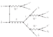
(a) Two top, three W

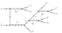
(b) One top, three W

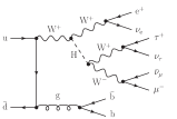
(c) Zero top, three W, Higgs

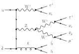
(d) Zero top, three W, Z

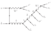
(e) Zero top, two W

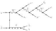
(f) Zero top, one W

Figure 1: Sample tree-level diagrams contributing to ${\text{t}\overline{\text{t}}}\text{W}^{+}$ production at the LHC.

In most of the diagrams, the propagating gluon is radiated from initial-state quarks and converts to ${\text{b}\overline{\text{b}}}$ [see for example Figs. 1(c), 1(d) and 1(f)]. However such diagrams give a small contribution to the squared amplitude, since they do not contain resonant top or antitop quarks. The leading contributions are provided by diagrams with a resonant ${\text{t}\overline{\text{t}}}$ pair, like the one depicted in Fig. 1(a). Also single-top-resonant diagrams like the one in Fig. 1(b) yield a visible contribution at LO. Other diagram topologies give minor contributions: a ${\text{W}^{+}\text{W}^{-}}$ pair can be produced via the decay of a Higgs [Fig. 1(c)] or a Z boson [Fig. 1(d)]. We observe that all diagrams contain at least one resonant $\text{W}^{+}$ boson.

2.1 Real corrections

Given the LO structure of the process, six possible partonic channels contribute to the real corrections at order ${\cal O}(\alpha_{\text{s}}^{3}\alpha^{6})$,

$$\text{u}\bar{\text{d}}/\text{c}\bar{\text{s}}\to{} \text{e}^{+}\nu_{\text{e}}\,\mu^{-}\bar{\nu}_{\mu}\,\tau^{+}\nu_{\tau}\,\text{b}\,\bar{}\text{b}\,\text{g}\,$$

$$\text{u}\text{g}/\text{c}\text{g}\to{} \text{e}^{+}\nu_{\text{e}}\,\mu^{-}\bar{\nu}_{\mu}\,\tau^{+}\nu_{\tau}\,\text{b}\,\bar{}\text{b}\,\text{d}/\text{s}\,$$

$$\text{g}\bar{\text{d}}/\text{g}\bar{\text{s}}\to{} \text{e}^{+}\nu_{\text{e}}\,\mu^{-}\bar{\nu}_{\mu}\,\tau^{+}\nu_{\tau}\,\text{b}\,\bar{}\text{b}\,{\bar{\text{u}}/\bar{\text{c}}}\,.$$ (2)

Since we consider a final state with three charged leptons, the additional gluon can only be radiated off the initial-state quark lines, the final-state b jets, or internal light-quark, bottom and top-quark propagators. For each real-radiation channel 1916 Feynman diagrams contribute. The $q\bar{q}^{\prime}$ channel is the one featuring the largest number of infrared (IR) singular regions, and thus is the most demanding in the numerical calculation. We treat bottom quarks as massless particles and work in the five-flavour scheme. For the final states of the processes (2.1), no initial states involving bottom quarks contribute for a diagonal quark-mixing matrix that we assume.

We treat the IR singularities with the Catani–Seymour subtraction scheme Catani:1996vz . The initial-state collinear QCD singularities are absorbed in the PDFs via the $\overline{{\text{MS}}}$ scheme. The spin-correlated and colour-correlated matrix elements entering the unintegrated subtraction counterterms are computed with Recola Actis:2012qn ; Actis:2016mpe . As a validation of the correct computation of the subtracted real and integrated counterterms, we have varied the $\alpha_{\text{dipole}}$ parameters Nagy:2003tz in the definition of the dipoles, as is further explained in Section 2.4.

Although computing the virtual contributions involves the evaluation of complicated one-loop diagrams (see the following section), the numerical simulation of the (subtracted) real contributions to NLO observables represents the most CPU-intensive part of the calculation, in spite of its tree-level nature and the relatively small number of QCD subtraction dipoles. This is due to the large multiplicity of the final state (three coloured partons, six leptons) but also due to the relatively small numerical contribution of the virtual corrections. Tackling the NLO EW corrections for the same process will be even more challenging, as the number of QED dipoles is larger than the one of QCD dipoles.

2.2 Virtual corrections

The virtual QCD corrections are obtained by inserting a gluon in the tree-level amplitudes, resulting in roughly 6000 Feynman diagrams for each partonic channel. The most complicated one-loop contributions involve 7-point functions appearing when a virtual gluon connects the initial-state light quarks and a final-state b quark in diagrams which do not feature the $\text{t}\overline{\text{t}}$ resonance structure. An example is depicted in Fig. 2.

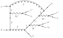
Figure 2: Sample one-loop diagram contributing to hadronic ${\text{t}\overline{\text{t}}}\text{W}^{+}$ production at NLO QCD involving a 7-point function.

The virtual corrections to the considered process are computed with SM amplitudes provided by Recola Actis:2012qn ; Actis:2016mpe interfaced to the Collier library Denner:2016kdg for the numerical evaluation of scalar and tensor one-loop integrals. All unstable particles are treated in the complex-mass scheme Denner:1999gp ; Denner:2000bj ; Denner:2005fg ; Denner:2006ic , resulting in complex input values for the electroweak boson masses, the top-quark mass, and the electroweak mixing angle,

$$\mu_{V}^{2}=M_{V}^{2}-\mathrm{i}\Gamma_{V}M_{V}\quad(V={\text{W},\text{Z}})\,,\qquad\mu_{\text{t}}^{2}=m_{\text{t}}^{2}-\mathrm{i}\Gamma_{\text{t}}m_{\text{t}}\,,\qquad\cos^{2}\theta_{{\mathrm{w}}}=\frac{\mu_{\text{W}}^{2}}{\mu_{\text{Z}}^{2}}\,.$$ (3)

2.3 Double-pole approximation

The hadronic process defined in Eq. (1) is dominated by the resonant production of a top–antitop-quark pair in association with a $\text{W}^{+}$ boson. Most of the results that are present in the literature Frederix:2017wme ; Frixione:2015zaa ; Maltoni:2014zpa ; Maltoni:2015ena ; Broggio:2016zgg ; Kulesza:2018tqz ; Kulesza:2020nfh ; Broggio:2019ewu are inclusive, i.e. they rely on the on-shell production of the three massive particles. More refined techniques have been investigated to complement the inclusive results with spin correlations and off-shell effects, without computing the full off-shell process, e.g. using the narrow-width approximation Campbell:2012dh ; Frederix:2020jzp . Such approximations help in assessing the importance of resonance structures as well as in validating parts of the full calculation.

A universal technique for processes dominated by a pair of resonances is the so-called double-pole approximation (DPA), which has been widely used in the literature for the calculation of NLO EW virtual corrections to several processes, like di-boson Denner:1997ia ; Jadach:1996hi ; Jadach:1998tz ; Beenakker:1998gr ; Billoni:2013aba ; Denner:2000bj , vector-boson scattering Biedermann:2016yds and top–antitop pair production Denner:2016jyo . In general, the pole approximation Stuart:1991xk ; Denner:2019vbn amounts to selecting all diagrams containing the resonance structure that is expected to be dominant in the full process. The Breit–Wigner modulation of the selected resonances is preserved with off-shell kinematics, while in the rest of the amplitude the resonant particles are treated with on-shell kinematics, obtained by means of properly defined projections. While the DPA is applied to the virtual contributions, the Born and real contributions to the NLO calculation are usually computed with full matrix elements Denner:2000bj . The extension of this technique to QCD corrections is straightforward.

We have applied a DPA to the top and antitop resonances in order to mimic as much as possible the on-shell calculations that are available in the literature for ${\text{t}\overline{\text{t}}\text{W}}$ production. The QCD corrections affect top quarks, being coloured particles, both in the production and in the decay parts of the amplitude. Therefore, both factorisable and non-factorisable gluonic corrections contribute to the resonant production of a ${\text{t}\overline{\text{t}}}$ pair. The factorisable corrections can be written in the general form

$${\cal M}^{I\rightarrow F_{a}F_{b}}_{\rm virt,fact}=\\ \sum_{h_{a},h_{b}}\frac{{\cal M}^{I\rightarrow a\,b}_{\rm virt}\,{\cal M}^{a\rightarrow F_{a}}_{\rm LO}\,{\cal M}^{b\rightarrow F_{b}}_{\rm LO}+{\cal M}^{I\rightarrow a\,b}_{\rm LO}\,{\cal M}^{a\rightarrow F_{a}}_{\rm virt}\,{\cal M}^{b\rightarrow F_{b}}_{\rm LO}+{\cal M}^{I\rightarrow a\,b}_{\rm LO}\,{\cal M}^{a\rightarrow F_{a}}_{\rm LO}\,{\cal M}^{b\rightarrow F_{b}}_{\rm virt}}{\left(s_{a}-m_{\text{t}}^{2}+\mathrm{i}m_{\text{t}}\Gamma_{\text{t}}\right)\,\left(s_{b}-m_{\text{t}}^{2}+\mathrm{i}m_{\text{t}}\Gamma_{\text{t}}\right)}\,,$$ (4)

where $s_{a},s_{b}$ and $h_{a},h_{b}$ stand for the virtualities and helicities of the intermediate top and antitop quarks, respectively. Further, ${\cal M}^{I\rightarrow a\,b}$, ${\cal M}^{a\rightarrow F_{a}}$, ${\cal M}^{b\rightarrow F_{b}}$ are the $\text{t}\overline{\text{t}}$ production amplitude and the top- and antitop-quark decay amplitudes. The non-factorisable corrections to the resonant amplitude have a universal structure Denner:1997ia ; Accomando:2004de ; Dittmaier:2015bfe ,

$$2\,{\rm Re}\left({\cal M}_{\rm LO}^{*}\,{\cal M}_{\rm virt,nfact}\right)=\left|{\cal M}_{\rm LO}\right|^{2}\,\delta_{\rm nfact}\,,$$ (5)

and are needed for the complete subtraction of IR singularities, since the real contributions are not treated with the pole approximation Denner:1997ia . Sample diagrams for factorisable and non-factorisable QCD corrections are shown in Fig. 3.

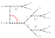
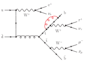
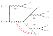
Figure 3: Sample diagrams for virtual corrections to hadronic ${\text{t}\overline{\text{t}}}\text{W}^{+}$ production: factorisable corrections to the top-quark production (left) and decay (middle), non-factorisable corrections (right).

The on-shell kinematics for the resonant contributions is obtained by suitable projections of the momenta, which involve some ambiguity. We employ on-shell projections for top quarks that preserve the off-shell-ness of the corresponding W bosons, in the same fashion as in Ref. Denner:2014wka .

In $\text{t}\overline{\text{t}}\text{W}^{+}$ production two virtual $\text{W}^{+}$ bosons appear, one of which results from the top-quark decay. Thus, the DPA receives two distinct contributions, one where the top quark decays into $\text{e}^{+}\nu_{\text{e}}\text{b}$ and one where it decays into $\tau^{+}\nu_{\tau}\text{b}$. Since the interference of these contributions is not doubly resonant, the full contributions in DPA are simply obtained upon adding these two contributions.

One last remark concerns the definition of the part of the NLO corrections that is calculated in the DPA. In the original DPA computations Denner:2000bj and in most computations performed with MoCaNLO Denner:2016jyo ; Denner:2016wet ; Biedermann:2016yds the DPA has been applied to the finite sum of the virtual corrections and the $I$-operator of the integrated Catani–Seymour dipoles, while the $P$- and $K$-operators have been calculated with off-shell kinematics. In this way, the infrared singularities are cancelled exactly, but the finite parts become scheme dependent. Nonetheless, the scheme dependence is of the order of the intrinsic uncertainty of the DPA (see Section 2.3 of Ref. Denner:2000bj ) and thus does not deteriorate the approximation. However, when done in combination with a small $\alpha_{\text{dipole}}$ parameter Nagy:1998bb , enhanced finite contributions in the subtracted and re-added real corrections are treated differently, which increases the error of the DPA and tends to worsen the agreement with the full computation Denner:2020bcz . This can be cured in different ways. One possibility is to calculate only the $\alpha_{\text{dipole}}$-independent part of the $I$-operators, i.e. the one for $\alpha_{\text{dipole}}=1$, within the DPA but the $\alpha_{\text{dipole}}$-dependent part, which contains logarithms of $\alpha_{\text{dipole}}$, with full kinematics. This allows to cancel exactly the $\alpha_{\text{dipole}}$-dependence in the sum of integrated and subtraction dipoles. Another option is to apply the DPA only to the virtual corrections with IR singularities subtracted via an appropriate choice of regularisation parameters. Since the virtual corrections are smaller than the contributions of the integrated dipoles, as shown in Section 3.4, this provides actually a better approximation of the calculation with full matrix elements.

2.4 Validation

The calculation presented in this paper has been validated at several levels.

The correct functioning of the subtraction of IR singularities has been checked performing the computation with different values of the $\alpha_{\text{dipole}}$ parameters that enter the calculation of integrated and unintegrated subtraction dipoles Nagy:2003tz . Setting $\alpha_{\text{dipole}}<1$ enables one to restrict the phase-space integration to the singular regions, in order to avoid problems from sizeable remappings of momenta in the Monte Carlo integration. Varying these parameters is equivalent to changing the definition of the subtraction counterterms, but the sum of the subtracted real and integrated dipoles remains independent of the choice of $\alpha_{\text{dipole}}$.

As a validation of the virtual contributions, we have compared the results based on full matrix elements with the corresponding DPA results, including factorisable and non-factorisable QCD corrections (see Section 2.3). The agreement between the two results is astonishingly good. At the integrated level, the discrepancy between the two calculations is of order $0.2\%$. A more detailed discussion on this comparison is given in Section 3.4.

The specific final state that we consider features three charged leptons with different flavours. However, in order to further check the computations with full matrix elements, we have independently reproduced some results that have been recently published in Ref. Bevilacqua:2020pzy , where the considered final state involves two identical positrons and a muon. Employing the same final state, SM input parameters, selection cuts ($p_{{\mathrm{T}},{b}}>25\,\text{GeV}$), PDF set (NNPDF3.0), as well as factorisation and renormalisation scale, we obtain the following integrated cross-sections:

$$\sigma_{\rm LO}={} 0.1147(1)^{+0.0304}_{-0.0224}\,{\,\text{fb}}\quad({\textrm{\mbox{Ref.~{}\cite[cite]{\@@bibref{Authors Phrase1YearPhrase2}{Bevilacqua:2020pzy}{\@@citephrase{(}}{\@@citephrase{)}}}}}}:0.1151^{+0.0305}_{-0.0225}\,{\,\text{fb}})\,,$$

$$\sigma_{\rm NLO}={} 0.1247(4)^{+0.0046}_{-0.0078}\,{\,\text{fb}}\quad({\textrm{\mbox{Ref.~{}\cite[cite]{\@@bibref{Authors Phrase1YearPhrase2}{Bevilacqua:2020pzy}{\@@citephrase{(}}{\@@citephrase{)}}}}}}:0.1244^{+0.0043}_{-0.0077}\,{\,\text{fb}})\,.$$

The only difference between the two calculations lies in the treatment of resonant electroweak vector bosons, which in Ref. Bevilacqua:2020pzy is performed in the fixed-width scheme, while in our calculation the complex-mass scheme is employed (see Section 2.2). The agreement between the two calculations is excellent, both at LO and at NLO QCD. This holds for the central values of the integrated cross-sections and for the theoretical uncertainties given by scale variations.

We have also studied some differential distributions in the setup of Ref. Bevilacqua:2020pzy , finding good agreement in the absolute distributions and in the shapes of relative corrections. In Fig. 4 we show the LO and NLO distributions in the variable $H_{{\mathrm{T}}}^{\rm vis}$ that is the scalar sum of the transverse momenta of all visible particles (excluding the additional radiated light jet), and for the rapidity–azimuthal-angle distance between the leading positron, i.e. the positron with highest transverse momentum, and the muon.

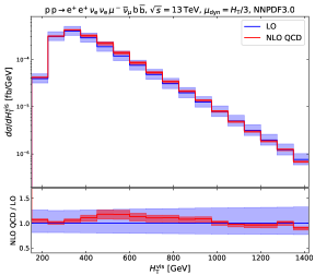
(a) $H_{{\mathrm{T}}}$ variable for visible particles (excluding additional light jet at NLO).

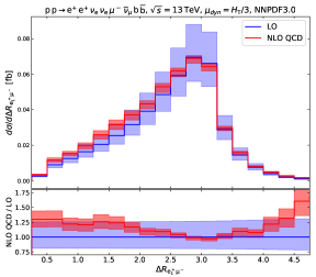
(b) Distance between the leading $p_{{\mathrm{T}}}$ positron and the muon.

Figure 4: Distributions at LO and NLO QCD for the process of Ref. Bevilacqua:2020pzy : differential cross-sections (upper plot) and $K$-factor (lower plot). The uncertainty bands have been computed by means of 7-point variations of the factorisation and renormalisation scale around the central scale.

From a direct comparison with Figs. 5 and 7 of Ref. Bevilacqua:2020pzy , we find the same dependence of the $K$-factors on the considered variables, as well as very similar scale uncertainty bands in the various kinematic regions. We have computed differential distributions in all of the kinematic variables that are presented in Ref. Bevilacqua:2020pzy , finding good agreement in all cases.

3 Numerical results

3.1 Input parameters

In the following, we present results for the LHC at a CM energy of 13 TeV. We consider a final state with three charged leptons of different flavours, which are all assumed to be massless, i.e. also $m_{\tau}=0$. We note that our results can be used as well for the case of identical leptons in the final state after applying appropriate symmetry factor $1/2$ up to interference effects. These interference effects are not doubly resonant and suppressed by factors $\Gamma_{\text{t}}/m_{\text{t}}$. However, calculating the NLO corrections for identical leptons does not pose any problems for our machinery and has in fact been done to compare with Ref. Bevilacqua:2020pzy , as described in Section 2.4. We work in the five-flavour scheme and treat all light quarks, including the b quarks, as massless. A unit Cabibbo-Kobayashi-Maskawa matrix is understood.

The on-shell values for the masses and widths of the electroweak bosons are chosen according to Ref. Tanabashi:2018oca :

$$M_{\text{W}}^{\text{OS}}={} 80.379\,\text{GeV},\qquad\,\,\,\Gamma_{\text{W}}^{\text{OS}}=2.085\,\text{GeV}\,,$$

$$M_{\text{Z}}^{\text{OS}}={} 91.1876\,\text{GeV},\qquad\Gamma_{\text{Z}}^{\text{OS}}\,=2.4952\,\text{GeV}\,,$$

$$M_{\text{H}}={} 125.00\,\text{GeV},\qquad\,\,\,\Gamma_{\text{H}}\,\,\,=0.00407\,\,\text{GeV}\,.$$ (6)

The masses of the vector bosons are converted to their pole values by means of the following relations Bardin:1988xt :

$$M_{V}=\frac{M^{\rm OS}_{V}}{\sqrt{1+({\Gamma^{\rm OS}_{V}}/{M^{\rm OS}_{V}})^{2}}}\,,\qquad\,\Gamma_{V}=\frac{\Gamma^{\rm OS}_{V}}{\sqrt{1+({\Gamma^{\rm OS}_{V}}/{M^{\rm OS}_{V}})^{2}}}\,.$$ (7)

The top-quark mass and widths are fixed as

$$m_{\text{t}}=173.0\,\text{GeV}\,,\qquad\Gamma_{\text{t}}^{\rm LO}=1.44\,\text{GeV}\,,\qquad\Gamma_{\text{t}}^{\rm NLO}=1.34\,\text{GeV}\,.$$ (8)

The top-quark width at LO has been computed based on the formulas of Ref. Jezabek:1988iv and using the pole mass and width for the W boson as input. The width at NLO QCD has been obtained upon applying the relative NLO QCD corrections of Ref. Basso:2015gca to the LO width.

The electroweak coupling is extracted from the Fermi constant $G_{\mu}$ Denner:2000bj by means of

$$\alpha=\frac{\sqrt{2}}{\pi}\,G_{\mu}M_{\text{W}}^{2}\left[1-\left(\frac{M_{\text{W}}^{2}}{M_{\text{Z}}^{2}}\right)\right]\,,$$ (9)

where $G_{\mu}=1.16638\cdot 10^{-5}\,\text{GeV}^{-2}$.

The masses of unstable particles, i.e. the electroweak vector bosons and the top quark are treated in the complex-mass scheme Denner:1999gp ; Denner:2000bj ; Denner:2005fg ; Denner:2006ic in all parts of the computation. As a consequence, the electroweak mixing angle and the couplings become complex as well.

For the LO (NLO) calculation, we use NNPDF3.1 PDFs Ball:2014uwa computed at LO (NLO) with $\alpha_{\text{s}}=0.118$. The strong coupling constant $\alpha_{\text{s}}$ used in the calculation of the amplitudes matches the one used in the evolution of PDFs. The PDFs and the running of $\alpha_{\text{s}}$ are obtained by interfacing MoCaNLO with LHAPDF6 Buckley:2014ana .

QCD partons with $|\eta|<5$ are clustered into jets by means of the anti-$k_{t}$ algorithm Cacciari:2008gp with resolution radius $R=0.4$.

Our choice of selection cuts reflects those applied by ATLAS in a recent analysis Aaboud:2019njj (see Table 5 therein). In particular, we ask for exactly two b jets in the final state, assuming a perfect b-tagging efficiency, which are required to fulfil

$$p_{{\mathrm{T}},{\text{b}}}>25\,\text{GeV}\,,\quad|\eta_{\text{b}}|<2.5\,.$$ (10)

We apply basic transverse-momentum, rapidity and isolation cuts to the three charged leptons,

$$p_{{\mathrm{T}},{\ell}}>27\,\text{GeV}\,,\quad|\eta_{\ell}|<2.5\,,\quad\Delta R_{\ell\text{b}}>0.4\,.$$ (11)

While these cuts are applied to the light leptons $\ell=\text{e},\mu$ by ATLAS, we apply them also to $\tau$ leptons. We remind the reader that our results can be applied as well for final states with identical leptons within a good approximation. No specific veto is imposed on the additional light jet that may come from real radiation at NLO QCD, in case it is not recombined with a b jet. Furthermore, we do not impose any restriction on the missing transverse momentum.

3.2 Fiducial cross-sections

A common choice in the literature for the factorisation and renormalisation scale for the considered process is deFlorian:2016spz ; Garzelli:2012bn

$$\mu_{0}^{\rm(a)}=m_{\text{t}}+\frac{M_{\text{W}}}{2}\,,$$ (12)

which is adapted to the masses of the leading resonance structure contributing to the final state under investigation. In addition to this fixed scale, we have considered dynamical scales that depend on the transverse momenta of the final-state particles. One choice depends on the $H_{{\mathrm{T}}}$ variable, defined as

$$H_{{\mathrm{T}}}=p_{{\mathrm{T}},{\rm miss}}+\sum_{i={\text{b},\ell}}p_{{\mathrm{T}},{i}}\,,$$

where the sum runs over all b jets and charged leptons, excluding additional light jets that may arise from real radiation at NLO. We have checked that the inclusion of the $p_{{\mathrm{T}}}$ of additional radiation would lead to a significant deterioration of the scale dependence of the fiducial cross-section. Since $H_{{\mathrm{T}}}$ is measurable at the LHC, it represents a natural scale choice in the computation of the full off-shell process. We have investigated two different variants of scales based on $H_{{\mathrm{T}}}$,

$$\mu_{0}^{\rm(b)}=\frac{H_{{\mathrm{T}}}}{2}\qquad{\rm and}\qquad\mu_{0}^{\rm(c)}=\frac{H_{{\mathrm{T}}}}{3}\,,$$ (13)

where the second one has been proposed in Ref. Bevilacqua:2020pzy .

An alternative definition of a dynamical scale is based on the top and antitop transverse masses, and is motivated by the choice made in Refs. Denner:2016wet ; Denner:2017kzu for $\text{t}\overline{\text{t}}$ and $\text{t}\overline{\text{t}}\text{H}$ production at the LHC,

$$\mu_{0}^{\rm(d)}={\left(M_{{\mathrm{T}},{\text{t}}}\,M_{{\mathrm{T}},{\overline{\text{t}}}}\right)}^{1/2}=\left(\sqrt{m_{\text{t}}^{2}+{p_{{\mathrm{T}},{\text{t}}}}^{2}}\,\sqrt{m_{\text{t}}^{2}+{p_{{\mathrm{T}},{\overline{\text{t}}}}}^{2}}\right)^{1/2}\,,$$ (14)

where the top and antitop transverse momenta are reconstructed from their decay products based on Monte Carlo truth. Note that the determination of the top momentum is subject to an ambiguity, since it can be reconstructed by two different lepton–neutrino pairs: we choose the pair that, combined with the b quark, gives rise to an invariant mass which is the closer to $m_{\text{t}}$. This scale choice is motivated by the expectation that top–antitop resonances dominate the cross-section, even when considering complete off-shell effects. Finally, we consider some results for the scale choice

$$\mu_{0}^{\rm(e)}=\frac{1}{2}{\left(M_{{\mathrm{T}},{\text{t}}}\,M_{{\mathrm{T}},{\overline{\text{t}}}}\right)}^{1/2}\,.$$ (15)

In Table 1 we show the integrated cross-sections for the five scale choices, complemented with the corresponding scale uncertainties, evaluated with 7-point scale variations, namely rescaling the central factorisation and renormalisation scale by the factors

$$\left(0.5,0.5\right),\left(1,0.5\right),\left(0.5,1\right),\left(1,1\right),\left(1,2\right),\left(2,1\right),\left(2,2\right)\,.$$

When performing scale variations, the NLO QCD top-quark width is kept fixed.

central scale	LO	NLO QCD	$K$-factor
$\mu_{0}^{\rm(a)}=m_{\text{t}}+{M_{\text{W}}}/{2}$	$0.2042(1)^{+0.0485(23.8\%)}_{-0.0367(18.0\%)}$	$0.2452(7)^{+0.0109(4.5\%)}_{-0.0166(6.8\%)}$	1.20
$\mu_{0}^{\rm(b)}=H_{{\mathrm{T}}}/2$	$0.1931(1)^{+0.0444(23.0\%)}_{-0.0339(17.5\%)}$	$0.2330(9)^{+0.0098(4.2\%)}_{-0.0152(6.5\%)}$	1.21
$\mu_{0}^{\rm(c)}=H_{{\mathrm{T}}}/3$	$0.2175(1)^{+0.0525(24.2\%)}_{-0.0396(18.2\%)}$	$0.2462(8)^{+0.0069(2.8\%)}_{-0.0143(5.8\%)}$	${1.13}$
$\mu_{0}^{\rm(d)}={\left(M_{{\mathrm{T}},{\text{t}}}\,M_{{\mathrm{T}},{\bar{\text{t}}}}\right)}^{1/2}$	$0.1920(1)^{+0.0441(23.0\%)}_{-0.0336(17.5\%)}$	$0.2394(6)^{+0.0129(5.4\%)}_{-0.0172(7.2\%)}$	1.25
$\mu_{0}^{\rm(e)}={\left(M_{{\mathrm{T}},{\text{t}}}\,M_{{\mathrm{T}},{\bar{\text{t}}}}\right)}^{1/2}/2$	$0.2360(1)^{+0.0591(24.9\%)}_{-0.0441(18.7\%)}$	$0.2535(8)^{+0.0086(3.4\%)}_{-0.0133(5.2\%)}$	1.07

Table 1: Fiducial cross-sections (fb) for fixed and dynamical scale choices defined in this section. The uncertainties have been computed with 7-point scale variations around the central value.

We have checked that the largest scale variations result from varying the renormalisation scale. At LO the fiducial cross-sections computed with $\mu_{0}^{\rm(b)}$ and $\mu_{0}^{\rm(d)}$ differ by less than $1\%$ and are about $6\%$ smaller than the results with fixed scale $\mu_{0}^{\rm(a)}$. The scale $\mu_{0}^{\rm(c)}$ gives a cross-section which is $6\%$ higher than the one obtained with the fixed scale, while the one for $\mu_{0}^{\rm(c)}$ is even $16\%$ larger. In all cases the scale uncertainties are of the same size, i.e. approximately $20\%$ relative to the central value. The QCD corrections amount to $+20\%$ for the fixed scale. While the scale $\mu_{0}^{\rm(b)}$ yields almost the same $K$-factor, the corrections are larger for $\mu_{0}^{\rm(d)}$ ($+25\%$) and smaller for $\mu_{0}^{\rm(c)}$ ($+13\%$) and $\mu_{0}^{\rm(e)}$ ($+7\%$). At NLO QCD, all scale choices give scale uncertainties of the order of $5\%$ with some small differences in the various cases. In particular, the use of $\mu_{0}^{\rm(c)}$ or $\mu_{0}^{\rm(e)}$ entails slightly smaller scale uncertainties compared to the fixed scale, while those of $\mu_{0}^{\rm(d)}$ are larger. These differences are more sizeable at the differential level, as is shown in the following.

In Fig. 5 we show the scale dependence of the fiducial cross-section for the five scale choices introduced in Eqs. (12)–(15).

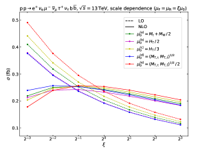
Figure 5: Scale dependence of the fiducial cross-section: factorisation and renormalisation scales are varied simultaneously about the central value $\mu_{0}$ with scale factor $\xi=\mu/\mu_{0}$.

The factorisation and renormalisation scales are varied simultaneously scaling the central value $\mu_{0}$ by a factor $\xi=1/8,1/4,1/2,1,2,4,8$. At LO, $\mu_{0}^{\rm(b)}$ and $\mu_{0}^{\rm(d)}$ give almost identical cross-sections for any $\xi$ factor, which are roughly $5\%$ smaller than the corresponding results with fixed scale $\mu_{0}^{\rm(a)}$. On the contrary, the scale $\mu_{0}^{\rm(c)}$ gives a $+6\%$ enhancement to the LO cross-sections with respect to the fixed scale. At NLO QCD, for $\xi>1$, the cross-section computed with $\mu_{0}^{\rm(a)}$ takes intermediate values between the corresponding value for $\mu_{0}^{\rm(c)}$ ($+7\%$) and for $\mu_{0}^{\rm(d)}$ ($-7\%$). The scale $\mu_{0}^{\rm(b)}$ behaves similarly to $\mu_{0}^{\rm(d)}$. At small values of the scales, $\xi<1$, the behaviour of the results for $\mu_{0}^{\rm(c)}$ and $\mu_{0}^{\rm(d)}$ is inverted: for the former the cross-section becomes noticeably lower than the one for fixed scale, while for the latter it becomes larger. Differently from $\mu_{0}^{\rm(d)}$, the results obtained with $\mu_{0}^{\rm(b)}$ for $\xi<1$ remain lower than those obtained with $\mu_{0}^{\rm(a)}$. The results for the central scale choice $\mu_{0}^{\rm(e)}=\mu_{0}^{\rm(d)}/2$ are close to those for $\mu_{0}^{\rm(c)}$, in particular for $\xi>1$. On the one hand, such a choice reduces the corresponding scale dependence by giving a flatter curve around the central value. Furthermore, it shifts the central scale towards the maximum of the curve in a similar way as going from $\mu_{0}^{\rm(b)}$ to $\mu_{0}^{\rm(c)}$ and leads to a smaller $K$-factor. On the other hand, $\mu_{0}^{\rm(d)}$ corresponds to the dynamical choice made in calculations for on-shell top quarks Denner:2016wet ; Denner:2017kzu .

3.3 Differential cross-sections

Beyond integrated cross-sections, it is of crucial importance to study how NLO QCD corrections affect the distributions in the relevant kinematic variables. This is the aim of this section. We start by comparing distributions obtained with different central-scale choices in Section 3.3.1 and the corresponding scale variation of the relative corrections. Thereafter we present more results for the dynamical scale $\mu_{0}^{\rm(d)}$ in Section 3.3.2.

3.3.1 Comparison of different central-scale definitions

Motivated by the results obtained at the integrated level, we are not showing any result for $\mu_{0}^{\rm(b)}$. The focus is put on the differences between the results obtained with the fixed scale and those obtained with $\mu_{0}^{\rm(c)}$ and $\mu_{0}^{\rm(d)}$, as we expect that the choice of a well-motivated dynamical scale is beneficial for a better behaviour of NLO QCD corrections, in particular, in the tails of energy-dependent distributions.

This is indeed the case for the transverse-momentum distributions for the positron and the reconstructed top quark, which are shown in Fig. 6 and Fig. 7, respectively.

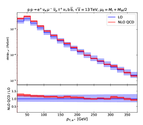
(a) Fixed scale $\mu_{0}^{\rm(a)}=m_{\text{t}}+M_{\text{W}}/2$.

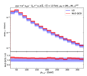
(b) Dynamical scale $\mu_{0}^{\rm(d)}={\left(M_{{\mathrm{T}},{\text{t}}}\,M_{{\mathrm{T}},{\bar{\text{t}}}}\right)}^{1/2}$.

Figure 6: Distributions in the transverse momentum of the positron at LO and NLO QCD: differential cross-sections (upper plot) and $K$-factor (lower plot). The uncertainty bands have been computed by means of 7-point variations of the factorisation and renormalisation scale around the central scale.

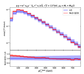
(a) Fixed scale $\mu_{0}^{\rm(a)}=m_{\text{t}}+M_{\text{W}}/2$.

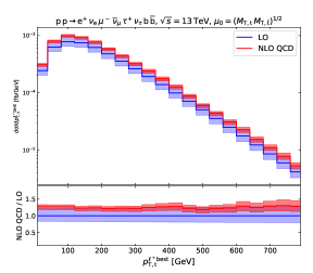
(b) Dynamical scale $\mu_{0}^{\rm(d)}={\left(M_{{\mathrm{T}},{\text{t}}}\,M_{{\mathrm{T}},{\bar{\text{t}}}}\right)}^{1/2}$.

Figure 7: Distributions in the transverse momentum of the reconstructed top quark at LO and NLO QCD: differential cross-sections (upper plot) and $K$-factor (lower plot). The uncertainty bands have been computed by means of 7-point variations of the factorisation and renormalisation scale around the central scale.

Comparing Fig. 6(a) with Fig. 6(b), it can be seen that using the fixed scale leads to a differential $K$-factor that drops monotonically from $1.25$ to $0.95$ with increasing transverse momentum of the positron. On the contrary, the dynamical scale gives a $K$-factor that decreases only from $1.3$ to $1.1$. Differently from the case of fixed scale, the scale uncertainties do not decrease for the dynamical scale in the tails of the distribution. Using the scale $\mu_{0}^{\rm(c)}$, the $K$-factor becomes somewhat flatter, but the scale uncertainties are similar.

The same situation can be found in the comparison of Fig. 7(a) and Fig. 7(b). The transverse momentum of the top quark considered in Fig. 7 refers to the top quark reconstructed using Monte Carlo truth from the bottom quark and the $\ell^{+}\nu_{\ell}$ pair that gives an invariant mass which is the closest to $m_{\text{t}}$ (denoted “$\ell^{+}$ best” in the following). While not measurable at the LHC, it is interesting to investigate this observable as it is directly related to the dominant resonant structure of the process, i.e. the top and antitop quarks. While the $K$-factor for the fixed scale drops from $1.35$ to $0.9$, it is practically flat for the dynamical scale $\mu_{0}^{\rm(d)}$. While the NLO uncertainty bands are similar in the two cases in the soft part of the spectrum they are sizeably larger for the dynamical scale at large transverse momentum. Again, the results are similar for the scale $\mu_{0}^{\rm(c)}$, where the $K$-factor varies from $1.20$ to $1.12$.

Given the flatness of the $K$-factors of Figs. 6 and 7, we can conclude that using the dynamical scale $\mu_{0}^{\rm(d)}$ or $\mu_{0}^{\rm(c)}$ results in better behaved NLO QCD corrections than with the fixed scale.

In Fig. 8 we consider the distribution in the $H_{{\mathrm{T}}}$ variable comparing the results obtained with the two dynamical scales $\mu_{0}^{\rm(d)}$ and $\mu_{0}^{\rm(c)}$.

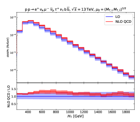
(a) Dynamical scale $\mu_{0}^{\rm(d)}={\left(M_{{\mathrm{T}},{\text{t}}}\,M_{{\mathrm{T}},{\bar{\text{t}}}}\right)}^{1/2}$

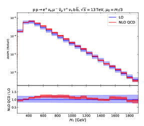
(b) Dynamical scale $\mu_{0}^{\rm(c)}=H_{{\mathrm{T}}}/3$

Figure 8: Distributions in the $H_{{\mathrm{T}}}$ variable at LO and NLO QCD: differential cross-sections (upper plot) and $K$-factor (lower plot). The uncertainty bands have been computed by 7-point variations of the factorisation and renormalisation scale around the central scale.

The dynamical scale $\mu_{0}^{\rm(d)}$, which depends on the top–antitop transverse masses, describes very well the $H_{{\mathrm{T}}}$ variable at NLO QCD, with a $K$-factor varying between $1.1$ and $1.35$. Furthermore, the $K$-factor has a similar shape and variation as the one obtained with $\mu_{0}^{\rm(c)}$, which coincides with the variable itself up to the 1/3 multiplicative factor. The most relevant difference between the two scales is given by a constant shift of the $K$-factor to larger values in the $\mu_{0}^{\rm(d)}$ case resulting from the difference of the integrated cross-section (see Table 1). The NLO uncertainty bands are marginally larger for $\mu_{0}^{\rm(d)}$ for moderate values of $H_{{\mathrm{T}}}$. We have checked numerically that the uncertainty bands for $\mu_{0}^{\rm(e)}$ are comparable to those for $\mu_{0}^{\rm(c)}$.

Since analogous similarities between the two scale choices can be found in the distributions for many other kinematic variables that we have investigated, we conclude that the quality of the NLO description of the process at the differential level is comparable for the two dynamical scale choices. Therefore, in all results we are going to present in the following, $\mu_{0}^{\rm(d)}$ is understood as a central factorisation and renormalisation scale.

3.3.2 Differential distributions for the default scale

In this section we discuss LO and NLO QCD results for selected differential cross-sections, including both angular and energy-dependent variables. We consider not only observables that are directly measurable at the LHC, but also kinematic variables related to the top and antitop resonances based on Monte Carlo truth. The explicit final state that we consider enables to sort charged leptons by their flavour, with no need of a transverse-momentum ordering. However, in order to be useful for final states with identical leptons, we also compute some observables based on the transverse-momentum ordering of the positively-charged leptons, as needed in the case of identical positrons Bevilacqua:2020pzy . We denote leptons or bottom quarks with highest transverse momenta as leading ones in the following. Moreover, we also sort the two positively-charged leptons $\text{e}^{+},\tau^{+}$ depending on how well they reconstruct the true top-quark invariant mass, as already done in the previous sections for the computation of the $\mu_{0}^{\rm(d)}$ central scale.

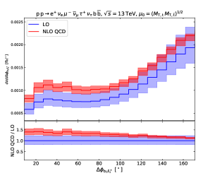
(a) Azimuthal separation between the leading b jet and the leading positively-charged lepton.

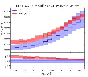
(b) Azimuthal separation between the positron and the muon.

Figure 9: Distributions at LO and NLO QCD for the dynamical scale choice: differential cross-sections (upper plot) and $K$-factor (lower plot). The uncertainty bands have been computed by means of 7-point variations of the factorisation and renormalisation scale around the central scale.

In Fig. 9 we show the LO and NLO distributions and $K$-factors for the azimuthal-angle separations between the leading b jet and the leading positively-charged lepton [both sorted by their $p_{{\mathrm{T}}}$, Fig. 9(a)] and between the positron and the muon [Fig. 9(b)]. The relative corrections for the two distributions behave similarly. In fact, the $K$-factors are of order $50\%$ in the region with smaller cross-section ($\Delta\phi\approx 0$) and decrease to $15\%$ towards $\Delta\phi=\pi$, where both distributions show a maximum. While the NLO uncertainty bands are almost as wide as the LO ones at low azimuthal separation, they become noticeably smaller in the peak region. We note that the distributions in the azimuthal separation between the antitau and the muon (which are not shown here) have exactly the same shape and normalisations as those shown in Fig. 9(b), since the leptonic decay of the $\text{W}^{+}$ boson is universal and the symmetry under the exchange of the two leptonically decaying $\text{W}^{+}$ bosons is accounted for in the full amplitudes. This comment holds for any variable that depends on the kinematics of a single positively-charged lepton selected by its flavour.

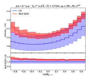
(a) Cosine of the angle between the two positively-charged leptons.

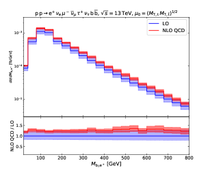
(b) Invariant mass of the system formed by the positron and the leading b jet.

Figure 10: Same as in Fig. 9.

A slightly different situation is found for the distribution in the cosine of the angle between the two positively charged leptons, shown in Fig. 10(a). This variable correlates the two charged leptons which are decay products of the two $\text{W}^{+}$ bosons, i.e. one of them comes from the top-quark decay and the other one from the $\text{W}^{+}$ boson recoiling against the $\text{t}\overline{\text{t}}$ system. The NLO corrections are positive over the whole spectrum, and inherit the relative increase in the cross-section from the integrated results ($+25\%$). The $K$-factor decreases from $1.4$ in the back-to-back configuration to $1.2$ in the collinear case. The minimum of the NLO distribution is shifted from $\cos\theta_{\text{e}^{+}\tau^{+}}\approx-0.35$ (at LO) to $-0.2$, and the two local maxima are in the collinear and anticollinear configurations: the former configuration is preferred, even though NLO corrections are larger for the latter.

In Fig. 10(b) we consider the distribution in the invariant mass of the system formed by the positron and the leading b jet. The distribution exhibits a maximum around $100\,\text{GeV}$ and a marked drop around $150\,\text{GeV}$. For on-shell W boson and top quark, this variable has an upper bound at $M_{\text{e}^{+}\text{b}}^{2}=m_{\text{t}}^{2}-M_{\text{W}}^{2}$. As the considered variable depends on the leading b jet, which is not necessarily the bottom quark that originates from the top quark, the drop is not as pronounced as it would be in the absence of this ambiguity. Nevertheless, the edge is present in the considered process and could help to increase the experimental sensitivity to the top-quark mass. In the on-shell region, $M_{\text{e}^{+}\text{b}}<150\,\text{GeV}$, the NLO QCD corrections mildly decrease from $30\%$ to $25\%$, while in the off-shell region, $M_{\text{e}^{+}\text{b}}>150\,\text{GeV}$, they basically reflect the overall normalisation with an almost flat $K$-factor, up to small statistical oscillations in the tails of the distribution where the rate is exponentially damped. The NLO uncertainty bands are of order $5\%$ in the part of the spectrum with a higher rate, while they increase to $15\%$ in the tails.

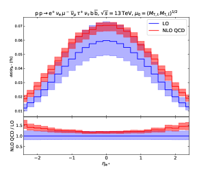
(a) Rapidity of the positron.

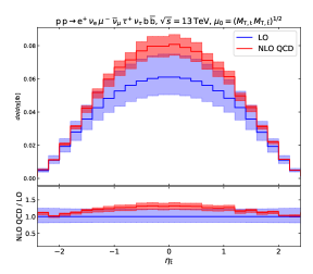
(b) Rapidity of the antitop quark.

Figure 11: Same as in Fig. 9.

In Fig. 11 we present the distributions in the rapidities of the positron and the antitop quark. The first distribution is measurable, while the second one is based on Monte Carlo truth. The positron rapidity is directly cut at $y_{\text{e}^{+}}=\pm 2.5$, while the one of the antitop gives an almost negligible contribution for $|y_{\bar{\text{t}}}|>2.5$. Despite having similar behaviours at LO, the effect of QCD radiative corrections is different in the two variables. In the positron case, the radiative corrections are maximal in the region close to the acceptance cut (roughly $+50\%$), while they are smaller near the peak of the distribution ($+20\%$ for $y_{\text{e}^{+}}=0$). In contrast, the radiative corrections give a maximal enhancement to the antitop distribution around the peak at zero rapidity ($+35\%$), while they are almost zero at large rapidities.

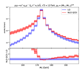
(a) Invariant mass of the antitop quark.

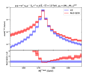
(b) Invariant mass of the reconstructed top quark.

Figure 12: Same as in Fig. 9.

In Figs. 12(a) and 12(b), we analyse the distributions in the invariant masses of the antitop quark and the reconstructed top quark, respectively. The top quark is reconstructed according to the above-described requirement that the selected $\ell^{+}\nu_{\ell}$ pair gives the invariant mass closest to $m_{\text{t}}$ when combined with the b-quark jet. In both cases, the NLO corrections are very large and positive below the top mass. For a reconstructed mass of $m_{\text{t}}-25\,\text{GeV}$, the NLO cross-section is one order of magnitude larger than the LO one. This radiative tail is due to final-state gluon radiation which is not recombined with the decay products of the antitop or top resonance. At the peak, the NLO corrections are small and negative ($-10\%$). In the off-shell region above the pole mass they become again large and positive, reaching $\approx+100\%$ at $m_{\text{t}}+25\,\text{GeV}$ for the reconstructed top quark. The relative corrections are more moderate for the antitop mass ($\approx 70\%$) in the same region owing to the absence of the reconstruction ambiguity which affects the top quark in the considered process. The general features of the correction to this distribution are similar as for top–antitop production Denner:2012yc .

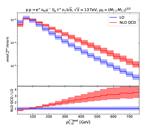
(a) Transverse momentum of the reconstructed ${\text{t}\overline{\text{t}}}$ system.

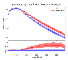
(b) Transverse momentum of the $\text{b}\bar{\text{b}}$ system.

Figure 13: Same as in Fig. 9.

As already seen in Fig. 12, not all distributions receive NLO $K$-factors that are close to the value of $1.25$ for the fiducial cross-section. In Fig. 13 we consider two more observables that experience very large NLO corrections in the tails of distributions, the transverse momentum of the $\text{t}\overline{\text{t}}$ system (depending on the reconstructed top quark) and the transverse momentum of the two b-jet system shown in Fig. 13(a) and Fig. 13(b), respectively. The transverse momentum of the top–antitop system is equivalent to the transverse momentum of the recoiling system formed by a $\text{W}^{+}$ boson and the additional light jet that may arise at NLO. The presence of a large real-radiation contribution explains the huge QCD corrections, which are of order $+200\%$ for values larger than $500\,\text{GeV}$. In this region the relative scale uncertainties are larger than the LO ones, since the dominant scale uncertainty arises from the real corrections of order $\alpha_{\text{s}}^{3}$ which have only LO accuracy. In the soft region of the spectrum the NLO corrections become negative. The transverse momentum of the $\text{b}\bar{\text{b}}$ system (which is measurable at the LHC) is less directly affected by the additional QCD radiation at NLO. For $p_{{\mathrm{T}},{\text{b}\bar{\text{b}}}}<150\,\text{GeV}$ the $K$-factor stays almost constant around $+20\%$, while for larger values it increases, exceeding $+100\%$ for $p_{{\mathrm{T}},{\text{b}\bar{\text{b}}}}>300\,\text{GeV}$. Also this large effect is due to the sizeable contribution of the real radiation which is not clustered into any of the two b jets. As for the ${\text{t}\overline{\text{t}}}$ system, the scale uncertainties are large in the tails of the distribution, as they are dominated by only LO accurate real radiation. We have checked that the differential $K$-factors and scale uncertainties for the two transverse-momentum distributions practically do not change if either $\mu_{0}^{\rm(c)}$ or $\mu_{0}^{\rm(e)}$ is used as a central scale.

3.4 Comparison with double-pole approximation

In the previous section we have investigated differential variables related to the top and antitop resonances of the process as well as variables that are measurable at the LHC, without having any direct connection to the dominant resonances.

Since performing the full computation is demanding from the computational point of view, approximated calculations are often used. For them, a proper validation is mandatory as they usually rely on on-shell approximations, which could in principle be far from reproducing the off-shell structure of the simulated processes.

In this section we compare integrated and differential results obtained with the full off-shell computation and those obtained with two different variants of the DPA described in Section 2.3. In one approach, we have applied the DPA to the virtual contributions only, obtaining impressive agreement with the full results. Alternatively, we have applied it both to the virtual corrections and to the $\alpha_{\text{dipole}}$-independent contributions of $I$-operators (see Section 2.3).

In Table 2 we show the different contributions to the fiducial NLO cross-sections, computed with full matrix elements and with the DPA.

contribution	full	DPA	$\Delta_{\rm DPA}$
B (Born, with NLO PDFs)	$~{}0.20326(4)$	$~{}0.19770(3)$	$-2.7\%$
V (virtual)	$-0.02079(5)$	$-0.02071(3)$	$-0.4\%$
I (integrated dipoles,
${\alpha_{\text{dipole}}}$-independent $I$-operator)	$-0.1004(1)$	$-0.0976(1)$	$-2.8\%$
I (integrated dipoles,
${\alpha_{\text{dipole}}}$-dependent $I$-operator, ${\alpha_{\text{dipole}}}=0.01$)	$-0.3276(3)$	$-0.3204(3)$	$-2.2\%$
I (integrated dipoles, $K,P$-operators, ${\alpha_{\text{dipole}}}=0.01$)	$~{}0.1682(2)$	–	–
R (real subtracted)	$~{}0.3167(5)$	–	–

Table 2: Contributions to the fiducial NLO cross-sections (fb), obtained with the off-shell calculation and with the DPA. The central scale $\mu_{0}^{\rm(d)}$ is understood. Numerical uncertainties are shown in parentheses. The value $\Delta_{\rm DPA}$ is computed as the difference between the DPA and the full results normalised to the full one.

The DPA underestimates the Born cross-section by $2.7\%$. Since the deviations from the full results can be very large in some kinematic regions, we are not showing differential distributions at Born level. The virtual contributions are very well described by the DPA, while the $\alpha_{\text{dipole}}$-independent and $\alpha_{\text{dipole}}$-dependent terms of the $I$-operators (which take negative values) are reproduced with $2.8\%$ and $2.2\%$ negative deviation, respectively, similarly to the LO contributions and of the expected order $\Gamma_{\text{t}}/m_{\text{t}}$.

The fiducial NLO cross-sections obtained with the full off-shell and the two DPA calculations read:

$$\sigma_{\rm NLO}^{\rm full}=0.2394(6)^{+5.4\%}_{-7.2\%}{\,\text{fb}}\,,\quad\sigma_{\rm NLO}^{\rm DPA,\,V}=0.2395(7)^{+5.8\%}_{-7.4\%}{\,\text{fb}}\,,\quad\sigma_{\rm NLO}^{\rm DPA,\,V+I}=0.2422(7)^{+6.3\%}_{-7.6\%}\,.$$

The uncertainty of the DPA approximation can be estimated by multiplying the generic relative uncertainty of the DPA of $\mathcal{O}(\Gamma_{\text{t}}/m_{\text{t}})$ with the absolute size of the terms that are approximated. Since the finite virtual corrections contribute less than $10\%$ to the NLO fiducial cross-section, the DPA uncertainty of $\sigma_{\rm NLO}^{\rm DPA,\,V}$ is of the order $10\%\times\Gamma_{\text{t}}/m_{\text{t}}\approx 0.1\%$. The difference to the full results turns out to be somewhat smaller. Since the integrated dipoles make up $50\%$ of the NLO cross-section, treating them in DPA yields an uncertainty of the order of $50\%\times\Gamma_{\text{t}}/m_{\text{t}}\approx 0.5\%$. The cross section $\sigma_{\rm NLO}^{\rm DPA,\,V+I}$ differs from the full NLO one by $1.2\%$, which is of the same order of magnitude. Treating also the $\alpha_{\text{dipole}}$-dependent integrated-dipole contributions within the DPA, would deteriorate the accuracy even more since these contributions are even larger but cancel to a large extent with the real subtracted contributions that are not treated with the DPA (see Table 2). This option is not considered any further in this paper. The percent-level discrepancy between $\sigma_{\rm NLO}^{\rm DPA,\,V+I}$ and $\sigma_{\rm NLO}^{\rm full}$ translates to even larger discrepancies when looking at exclusive phase-space regions. Note that in both DPA calculations, the scale variations give slightly larger scale uncertainties than in the full calculation.

In Fig. 14 we consider the transverse-momentum and invariant-mass distributions of the two-b-jet system.

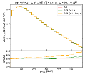
(a) Transverse momentum of the $\text{b}\bar{\text{b}}$ system.

(b) Invariant mass of the $\text{b}\bar{\text{b}}$ system.

Figure 14: Differential distributions at NLO QCD, obtained with full matrix elements, and applying the DPA either to the virtual contributions only, or both to the virtual and to the $\alpha_{\text{dipole}}$-independent part of $I$-operators. The dynamical scale $\mu_{0}^{\rm(d)}={\left(M_{{\mathrm{T}},{\text{t}}}\,M_{{\mathrm{T}},{\bar{\text{t}}}}\right)}^{1/2}$ is understood. Differential cross-sections are shown in the upper plot, the ratio over the full result in the lower plot.

Discrepancies at the level of $5\%$ can be found in the tails of the two distributions, though with opposite signs, when approximating the virtual corrections. The DPA gives a larger NLO cross-section in the large-transverse-momentum regime and a smaller one for large invariant masses. In Ref. Bevilacqua:2020pzy , an analogous effect of even $20\%$ has been found in the invariant-mass spectrum using the narrow-width approximation. Applying the DPA also to the integrated dipoles shifts the results towards larger values in the tails of both distributions, resulting in a $+10\%$ deviation for $p_{{\mathrm{T}},{\text{b}\bar{\text{b}}}}=600\,\text{GeV}$, and in a deviation of $2\%$ at large invariant mass ($M_{\text{b}\bar{\text{b}}}>200\,\text{GeV}$). In the tails of the distributions, the relative contribution of integrated dipoles to the cross-section is even larger than at the integrated level.

To investigate how well the top-quark resonance is reproduced within the DPA, we consider the distribution in the invariant mass of the positron–electron-neutrino–bottom system, $M_{\text{e}^{+}\nu_{\text{e}}\text{b}}$, and of the reconstructed (with the same criterion as used in the previous sections) top quark in Fig. 15.

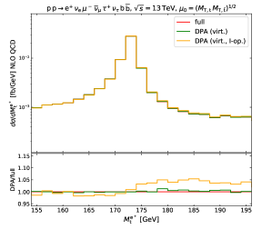
(a) Invariant mass of the positron–electron-neutrino–bottom system.

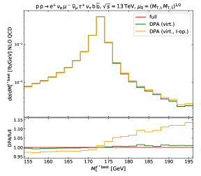
(b) Invariant mass of the reconstructed top quark.

Figure 15: Same as in Fig. 14.

The DPA applied to virtual corrections only leads to a result that is slightly smaller (larger) than the full one for invariant masses below (above) the top-quark mass. However, this effect is very small (at most $1\%$) for both variants of the reconstructed top quark mass. Applying the DPA to integrated dipoles affects the two distributions differently for values larger than $m_{\text{t}}$. For $M_{\text{e}^{+}\nu_{\text{e}}\text{b}}$, the DPA result is $5\%$ larger than the full result in this region, while choosing the reconstructed top-quark mass gives a larger deviation reaching $+13\%$ for $M_{\text{t}}^{\ell^{+}\,\rm best}=m_{\text{t}}+20\,\text{GeV}$. The large deviations appear in the off-shell region above the top resonance in which the resonant contributions are suppressed. The effect is smaller in Fig. 15(a) because of the background of about half of the events, where the resonant top-quark decays to $\text{b}\tau^{+}\nu_{\tau}$.

The distribution in the $H_{{\mathrm{T}}}$ observable is considered in Fig. 16(a).

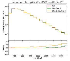
(a) $H_{{\mathrm{T}}}$ variable, excluding additional radiation.

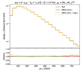
(b) Transverse momentum of the antitop quark.

Figure 16: Same as in Fig. 14.

The DPA calculation gives a relevant enhancement to the off-shell result in the tail of the distribution. The size of this effect for $H_{{\mathrm{T}}}>1600\,\text{GeV}$ is $3\%$ if the DPA is applied only to the virtual contributions and $7\%$ if it is applied also to the integrated dipoles. The deviation has some similarities with the one observed in the $\text{b}\bar{\text{b}}$ system transverse momentum [see Fig. 14(a)]. The $H_{{\mathrm{T}}}$ variable has been studied in Ref. Bevilacqua:2020pzy , finding that the narrow-width approximation underestimates the full cross-section for large $H_{{\mathrm{T}}}$ by some $30\%$, going in the opposite direction with respect to the DPA technique we consider here. This highlights that approximated computations should be taken with a grain of salt, and must be verified with results based on full matrix elements, in particular, in regions of phase space where non-doubly-resonant contributions are not suppressed.

As a last example, we show the distributions in the antitop-quark transverse momentum in Fig. 16(b). This variable is well described by the DPA in the whole spectrum, even in the tail. The discrepancy between the two DPA curves and the full one is roughly constant and reflects the results at the integrated level. This illustrates that the DPA works very well also at the differential level for kinematic variables that are directly related to the antitop or top quark. Both for the DPA applied to only the virtual corrections and the DPA applied also to the contributions of the $I$-operators the relative deviations from the off-shell results are flat and of the same size as for the fiducial cross-section.

4 Conclusions

In this paper, we have presented the calculation of NLO QCD corrections to the off-shell production of a top–antitop-quark pair in association with a $\text{W}^{+}$ boson, considering a final state with three charged leptons, two b jets and missing energy. Although our results have been obtained for the specific case of three different lepton flavours, they hold to good approximation also for the case of two identical positively-charged leptons up to a global symmetry factor 1/2. All non-resonant effects, interferences, as well as spin correlations are accounted for in all parts of the computation. We have studied both integrated and differential cross-sections, and performed a comparison between the results obtained from full matrix elements and those obtained using a double-pole approximation (DPA).

We have investigated different choices of the central factorisation and renormalisation scale, both fixed and dynamical. We have found that employing a dynamical scale gives better-behaved NLO QCD predictions than using the fixed scale $\mu_{0}=m_{\text{t}}+M_{\text{W}}/2$. This holds both for a scale based on the transverse-momentum content of the final state, $\mu_{0}=H_{{\mathrm{T}}}$, and for a scale based on the transverse masses of the dominant top–antitop resonances, $\mu_{0}=(M_{\text{t},{\mathrm{T}}}\,M_{\bar{\text{t}},{\mathrm{T}}})^{1/2}$.

Considering proton–proton collisions at a $13\,\text{TeV}$, the QCD corrections with a dynamical scale choice are positive and moderate ($+25\%$) at the integrated level. The theoretical uncertainties estimated from scale variations decrease from $20\%$ at LO to $5\%$ at NLO. Corrections for distribution become larger than those for the fiducial cross-section in several phase-space regions, in particular, in the tails of energy-dependent distributions which depend on the hadronic activity (b jets, additional QCD radiation), both for measurable LHC observables and for variables based on Monte Carlo truth describing the top and antitop resonances. The scale uncertainties are of the same or even larger size than the LO ones in the tails of certain transverse-momentum and invariant-mass distributions.

The DPA reproduces in a surprisingly accurate manner most results of the calculation based on full matrix elements if applied only to the virtual corrections, thanks to the relatively small size of such contributions. When the DPA is applied also to the integrated subtraction counterterms ($I$-operators in the Catani–Seymour scheme), it reproduces the full results at the $1\%$ level for the fiducial cross-section and top-dependent observables, while deviations of a few percent are found in more exclusive parts of the phase space, in agreement with the intrinsic uncertainty of the approximation. However, in regions of phase space that are not dominated by top–antitop production, the discrepancy can reach $10\%$ and more.

In conclusion, the calculation presented in this paper represents an important step towards a precise theoretical description of ${\text{t}\overline{\text{t}}\text{W}}$ production, which will be beneficial both in direct searches and in the background modelling for other relevant signals at the LHC. Since off-shell $\text{t}\overline{\text{t}}\text{W}$ production is dominated by contributions from top and antitop resonances, the approximated calculation relying on the resonant contributions is expected to give a reasonable picture of the process in sufficiently inclusive phase-space regions. However, given the increased luminosity that will be available in the next LHC runs, in view of a precise and fully trustworthy comparison between experimental data and theoretical predictions, the calculation based on full matrix elements is strongly recommended, as it gives a more complete description of the process in inclusive and exclusive kinematic regions.

References

- (1) ATLAS Collaboration, G. Aad et al., Measurement of the and production cross sections in pp collisions at 8 TeV with the ATLAS detector, JHEP 11 (2015) 172, [1509.05276].
- (2) CMS Collaboration, V. Khachatryan et al., Observation of top quark pairs produced in association with a vector boson in pp collisions at 8 TeV, JHEP 01 (2016) 096, [1510.01131].
- (3) ATLAS Collaboration, M. Aaboud et al., Measurement of the and production cross sections in multilepton final states using 3.2 fb-1 of collisions at 13 TeV with the ATLAS detector, Eur. Phys. J. C77 (2017) 40, [1609.01599].
- (4) CMS Collaboration, A. M. Sirunyan et al., Measurement of the cross section for top quark pair production in association with a W or Z boson in proton-proton collisions at 13 TeV, JHEP 08 (2018) 011, [1711.02547].
- (5) ATLAS Collaboration, M. Aaboud et al., Measurement of the and cross sections in proton-proton collisions at 13 TeV with the ATLAS detector, Phys. Rev. D99 (2019) 072009, [1901.03584].
- (6) CMS Collaboration, A. M. Sirunyan et al., Measurement of top quark pair production in association with a Z boson in proton-proton collisions at 13 TeV, JHEP 03 (2020) 056, [1907.11270].
- (7) J. A. Dror, M. Farina, E. Salvioni, and J. Serra, Strong tW Scattering at the LHC, JHEP 01 (2016) 071, [1511.03674].
- (8) A. Buckley, C. Englert, J. Ferrando, D. J. Miller, L. Moore, M. Russell, and C. D. White, Constraining top quark effective theory in the LHC Run II era, JHEP 04 (2016) 015, [1512.03360].
- (9) O. Bessidskaia Bylund, F. Maltoni, I. Tsinikos, E. Vryonidou, and C. Zhang, Probing top quark neutral couplings in the Standard Model Effective Field Theory at NLO in QCD, JHEP 05 (2016) 052, [1601.08193].
- (10) M. Guchait and D. Roy, Like sign dilepton signature for gluino production at CERN LHC including top quark and Higgs boson effects, Phys. Rev. D 52 (1995) 133–141, [hep-ph/9412329].
- (11) R. Barnett, J. F. Gunion, and H. E. Haber, Discovering supersymmetry with like sign dileptons, Phys. Lett. B 315 (1993) 349–354, [hep-ph/9306204].
- (12) J. Aguilar-Saavedra, R. Benbrik, S. Heinemeyer, and M. Pérez-Victoria, Handbook of vectorlike quarks: Mixing and single production, Phys. Rev. D 88 (2013) 094010, [1306.0572].
- (13) M. Perelstein, Little Higgs models and their phenomenology, Prog. Part. Nucl. Phys. 58 (2007) 247–291, [hep-ph/0512128].
- (14) R. Chivukula, E. H. Simmons, and J. Terning, A heavy top quark and the vertex in non-commuting extended technicolor, Phys. Lett. B 331 (1994) 383–389, [hep-ph/9404209].
- (15) G. Bevilacqua, H. Hartanto, M. Kraus, T. Weber, and M. Worek, Towards constraining Dark Matter at the LHC: Higher order QCD predictions for , JHEP 11 (2019) 001, [1907.09359].
- (16) H. Baer, C.-h. Chen, F. Paige, and X. Tata, Signals for minimal supergravity at the CERN large hadron collider. 2: Multi-lepton channels, Phys. Rev. D 53 (1996) 6241–6264, [hep-ph/9512383].
- (17) F. M. L. Almeida Jr., Y. do Amaral Coutinho, J. A. Martins Simões, P. Queiroz Filho, and C. Porto, Same-sign dileptons as a signature for heavy Majorana neutrinos in hadron hadron collisions, Phys. Lett. B 400 (1997) 331–334, [hep-ph/9703441].
- (18) J. Maalampi and N. Romanenko, Single production of doubly charged Higgs bosons at hadron colliders, Phys. Lett. B 532 (2002) 202–208, [hep-ph/0201196].
- (19) R. Contino and G. Servant, Discovering the top partners at the LHC using same-sign dilepton final states, JHEP 06 (2008) 026, [0801.1679].
- (20) F. Maltoni, M. Mangano, I. Tsinikos, and M. Zaro, Top-quark charge asymmetry and polarization in production at the LHC, Phys. Lett. B 736 (2014) 252–260, [1406.3262].
- (21) F. Maltoni, D. Pagani, and I. Tsinikos, Associated production of a top-quark pair with vector bosons at NLO in QCD: impact on searches at the LHC, JHEP 02 (2016) 113, [1507.05640].
- (22) ATLAS Collaboration, M. Aaboud et al., Observation of Higgs boson production in association with a top quark pair at the LHC with the ATLAS detector, Phys. Lett. B 784 (2018) 173–191, [1806.00425].
- (23) CMS Collaboration, A. M. Sirunyan et al., Observation of H production, Phys. Rev. Lett. 120 (2018) 231801, [1804.02610].
- (24) ATLAS Collaboration Collaboration, Analysis of and production in multilepton final states with the ATLAS detector, Tech. Rep. ATLAS-CONF-2019-045, CERN, Geneva, Oct, 2019.
- (25) CMS Collaboration Collaboration, Search for Higgs boson production in association with top quarks in multilepton final states at 13 TeV, Tech. Rep. CMS-PAS-HIG-17-004, CERN, Geneva, 2017.
- (26) J. M. Campbell and R. K. Ellis, production and decay at NLO, JHEP 07 (2012) 052, [1204.5678].
- (27) M. V. Garzelli, A. Kardos, C. G. Papadopoulos, and Z. Trocsanyi, and Hadroproduction at NLO accuracy in QCD with Parton Shower and Hadronization effects, JHEP 11 (2012) 056, [1208.2665].
- (28) S. Frixione, V. Hirschi, D. Pagani, H. S. Shao, and M. Zaro, Electroweak and QCD corrections to top-pair hadroproduction in association with heavy bosons, JHEP 06 (2015) 184, [1504.03446].
- (29) R. Frederix, D. Pagani, and M. Zaro, Large NLO corrections in and hadroproduction from supposedly subleading EW contributions, JHEP 02 (2018) 031, [1711.02116].
- (30) H. T. Li, C. S. Li, and S. A. Li, Renormalization group improved predictions for production at hadron colliders, Phys. Rev. D 90 (2014) 094009, [1409.1460].
- (31) A. Broggio, A. Ferroglia, G. Ossola, and B. D. Pecjak, Associated production of a top pair and a W boson at next-to-next-to-leading logarithmic accuracy, JHEP 09 (2016) 089, [1607.05303].
- (32) A. Kulesza, L. Motyka, D. Schwartländer, T. Stebel, and V. Theeuwes, Associated production of a top quark pair with a heavy electroweak gauge boson at NLONNLL accuracy, Eur. Phys. J. C 79 (2019) 249, [1812.08622].
- (33) A. Broggio, A. Ferroglia, R. Frederix, D. Pagani, B. D. Pecjak, and I. Tsinikos, Top-quark pair hadroproduction in association with a heavy boson at NLO+NNLL including EW corrections, JHEP 08 (2019) 039, [1907.04343].
- (34) A. Kulesza, L. Motyka, D. Schwartländer, T. Stebel, and V. Theeuwes, Associated top quark pair production with a heavy boson: differential cross sections at NLO+NNLL accuracy, Eur. Phys. J. C 80 (2020) 428, [2001.03031].
- (35) R. Frederix and I. Tsinikos, Subleading EW corrections and spin-correlation effects in multi-lepton signatures, Eur. Phys. J. C 80 (2020), no. 9 803, [2004.09552].
- (36) G. Bevilacqua, H.-Y. Bi, H. B. Hartanto, M. Kraus, and M. Worek, The simplest of them all: at NLO accuracy in QCD, JHEP 08 (2020) 043, [2005.09427].
- (37) A. Denner and R. Feger, NLO QCD corrections to off-shell top-antitop production with leptonic decays in association with a Higgs boson at the LHC, JHEP 11 (2015) 209, [1506.07448].
- (38) A. Denner and M. Pellen, NLO electroweak corrections to off-shell top-antitop production with leptonic decays at the LHC, JHEP 08 (2016) 155, [1607.05571].
- (39) A. Denner and M. Pellen, Off-shell production of top-antitop pairs in the lepton+jets channel at NLO QCD, JHEP 02 (2018) 013, [1711.10359].
- (40) A. Denner, J.-N. Lang, M. Pellen, and S. Uccirati, Higgs production in association with off-shell top-antitop pairs at NLO EW and QCD at the LHC, JHEP 02 (2017) 053, [1612.07138].
- (41) S. Actis, A. Denner, L. Hofer, A. Scharf, and S. Uccirati, Recursive generation of one-loop amplitudes in the Standard Model, JHEP 04 (2013) 037, [1211.6316].
- (42) S. Actis, A. Denner, L. Hofer, J.-N. Lang, A. Scharf, and S. Uccirati, RECOLA: REcursive Computation of One-Loop Amplitudes, Comput. Phys. Commun. 214 (2017) 140–173, [1605.01090].
- (43) A. Denner, S. Dittmaier, and L. Hofer, COLLIER: a fortran-based Complex One-Loop LIbrary in Extended Regularizations, Comput. Phys. Commun. 212 (2017) 220–238, [1604.06792].
- (44) A. Denner and S. Dittmaier, Reduction of one-loop tensor 5-point integrals, Nucl. Phys. B 658 (2003) 175–202, [hep-ph/0212259].
- (45) A. Denner and S. Dittmaier, Reduction schemes for one-loop tensor integrals, Nucl. Phys. B 734 (2006) 62–115, [hep-ph/0509141].
- (46) A. Denner and S. Dittmaier, Scalar one-loop 4-point integrals, Nucl. Phys. B 844 (2011) 199–242, [1005.2076].
- (47) S. Catani and M. Seymour, A general algorithm for calculating jet cross-sections in NLO QCD, Nucl. Phys. B 485 (1997) 291–419, [hep-ph/9605323]. [Erratum: Nucl. Phys. B 510 (1998) 503–504].
- (48) Z. Nagy, Next-to-leading order calculation of three jet observables in hadron hadron collision, Phys. Rev. D 68 (2003) 094002, [hep-ph/0307268].
- (49) A. Denner, S. Dittmaier, M. Roth, and D. Wackeroth, Predictions for all processes , Nucl. Phys. B560 (1999) 33–65, [hep-ph/9904472].
- (50) A. Denner, S. Dittmaier, M. Roth, and D. Wackeroth, Electroweak radiative corrections to fermions in double pole approximation: The RACOONWW approach, Nucl. Phys. B587 (2000) 67–117, [hep-ph/0006307].
- (51) A. Denner, S. Dittmaier, M. Roth, and L. H. Wieders, Electroweak corrections to charged-current fermion processes: Technical details and further results, Nucl. Phys. B724 (2005) 247–294, [hep-ph/0505042]. [Erratum: Nucl. Phys. B 854 (2012) 504].
- (52) A. Denner and S. Dittmaier, The complex-mass scheme for perturbative calculations with unstable particles, Nucl. Phys. B Proc. Suppl. 160 (2006) 22–26, [hep-ph/0605312].
- (53) A. Denner, S. Dittmaier, and M. Roth, Non-factorizable photonic corrections to four fermions, Nucl. Phys. B519 (1998) 39–84, [hep-ph/9710521].
- (54) S. Jadach, W. Płaczek, M. Skrzypek, B. F. L. Ward, and Z. Wa̧s, Exact gauge invariant YFS exponentiated Monte Carlo for (un)stable production at and beyond LEP2 energies, Phys. Lett. B417 (1998) 326–336, [hep-ph/9705429].
- (55) S. Jadach, W. Płaczek, M. Skrzypek, B. F. L. Ward, and Z. Wa̧s, Final-state radiative effects for the exact Yennie-Frautschi-Suura exponentiated (un)stable production at and beyond LEP2 energies, Phys. Rev. D61 (2000) 113010, [hep-ph/9907436].
- (56) W. Beenakker, F. A. Berends, and A. P. Chapovsky, Radiative corrections to pair production of unstable particles: results for fermions, Nucl. Phys. B548 (1999) 3–59, [hep-ph/9811481].
- (57) M. Billoni, S. Dittmaier, B. Jäger, and C. Speckner, Next-to-leading order electroweak corrections to leptons at the LHC in double-pole approximation, JHEP 12 (2013) 043, [1310.1564].
- (58) B. Biedermann, A. Denner, and M. Pellen, Large electroweak corrections to vector-boson scattering at the Large Hadron Collider, Phys. Rev. Lett. 118 (2017) 261801, [1611.02951].
- (59) R. G. Stuart, Gauge invariance, analyticity and physical observables at the resonance, Phys. Lett. B 262 (1991) 113–119.
- (60) A. Denner and S. Dittmaier, Electroweak Radiative Corrections for Collider Physics, Phys. Rept. 864 (2020) 1–163, [1912.06823].
- (61) E. Accomando, A. Denner, and A. Kaiser, Logarithmic electroweak corrections to gauge-boson pair production at the LHC, Nucl. Phys. B 706 (2005) 325–371, [hep-ph/0409247].
- (62) S. Dittmaier and C. Schwan, Non-factorizable photonic corrections to resonant production and decay of many unstable particles, Eur. Phys. J. C 76 (2016) 144, [1511.01698].
- (63) A. Denner, R. Feger, and A. Scharf, Irreducible background and interference effects for Higgs-boson production in association with a top-quark pair, JHEP 04 (2015) 008, [1412.5290].
- (64) Z. Nagy and Z. Trócsányi, Next-to-leading order calculation of four-jet observables in electron-positron annihilation, Phys. Rev. D59 (1999) 014020, [hep-ph/9806317]. [Erratum: Phys. Rev. D 62 (2000) 099902].
- (65) A. Denner and G. Pelliccioli, Polarized electroweak bosons in production at the LHC including NLO QCD effects, 2006.14867.
- (66) Particle Data Group Collaboration, M. Tanabashi et al., Review of Particle Physics, Phys. Rev. D 98 (2018) 030001.
- (67) D. Yu. Bardin, A. Leike, T. Riemann, and M. Sachwitz, Energy-dependent width effects in annihilation near the Z-boson pole, Phys. Lett. B206 (1988) 539–542.
- (68) M. Jeżabek and J. H. Kühn, QCD Corrections to Semileptonic Decays of Heavy Quarks, Nucl. Phys. B314 (1989) 1–6.
- (69) L. Basso, S. Dittmaier, A. Huss, and L. Oggero, Techniques for the treatment of IR divergences in decay processes at NLO and application to the top-quark decay, Eur. Phys. J. C76 (2016) 56, [1507.04676].
- (70) NNPDF Collaboration, R. D. Ball et al., Parton distributions for the LHC Run II, JHEP 04 (2015) 040, [1410.8849].
- (71) A. Buckley, J. Ferrando, S. Lloyd, K. Nordström, B. Page, M. Rüfenacht, M. Schönherr, and G. Watt, LHAPDF6: parton density access in the LHC precision era, Eur. Phys. J. C 75 (2015) 132, [1412.7420].
- (72) M. Cacciari, G. P. Salam, and G. Soyez, The anti- jet clustering algorithm, JHEP 04 (2008) 063, [0802.1189].
- (73) LHC Higgs Cross Section Working Group Collaboration, D. de Florian et al., Handbook of LHC Higgs Cross Sections: 4. Deciphering the Nature of the Higgs Sector, 1610.07922. CERN-2017-002-M.
- (74) A. Denner, S. Dittmaier, S. Kallweit, and S. Pozzorini, NLO QCD corrections to off-shell top-antitop production with leptonic decays at hadron colliders, JHEP 1210 (2012) 110, [1207.5018].