Pixel-Pair Occlusion Relationship Map (P2ORM): Formulation, Inference & Application

Abstract

We formalize concepts around geometric occlusion in 2D images (i.e., ignoring semantics), and propose a novel unified formulation of both occlusion boundaries and occlusion orientations via a pixel-pair occlusion relation. The former provides a way to generate large-scale accurate occlusion datasets while, based on the latter, we propose a novel method for task-independent pixel-level occlusion relationship estimation from single images. Experiments on a variety of datasets demonstrate that our method outperforms existing ones on this task. To further illustrate the value of our formulation, we also propose a new depth map refinement method that consistently improve the performance of state-of-the-art monocular depth estimation methods. Our code and data are available at http://imagine.enpc.fr/~qiux/P2ORM/.

1 Introduction

Occlusions are ubiquitous in 2D images (cf. Fig. 1(a)) and constitute a major obstacle to address scene understanding rigorously and efficiently. Besides the joint treatment of occlusion when developing techniques for specific tasks [40, 19, 54, 36, 35, 37, 18], task-independent occlusion reasoning [42, 24, 49, 53, 51, 30] offers valuable occlusion-related features for high-level scene understanding tasks.

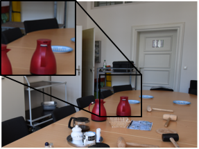
(a)

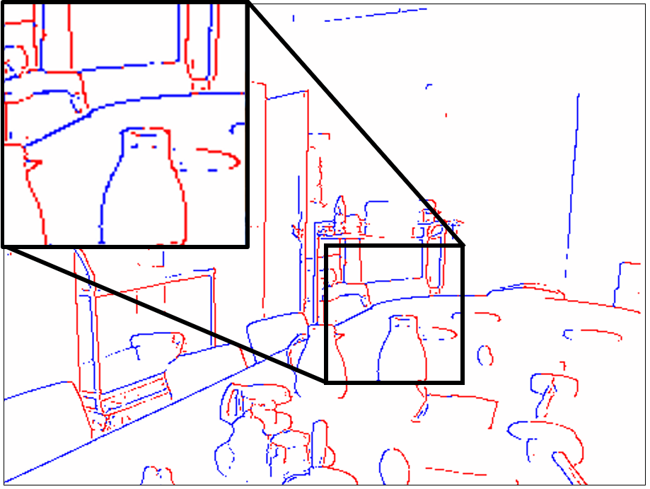
(b)

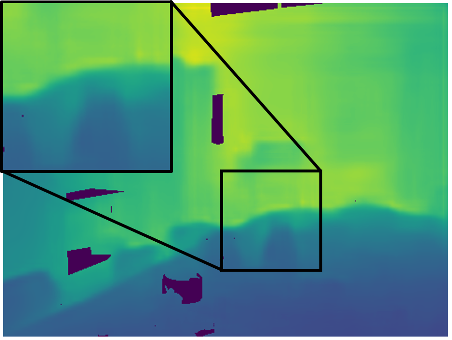
(c)

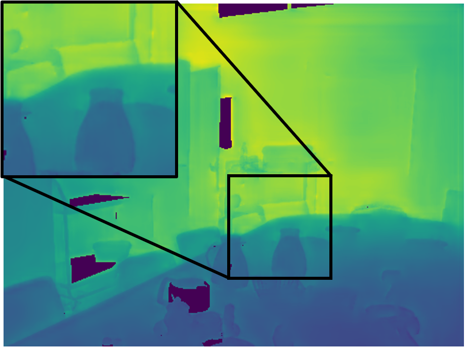
(d)

Figure 1: Illustration of the proposed methods: (a) input image, (b) estimated horizontal occlusion relationship (a part of P2ORM) where red (resp. blue) pixels occlude (resp. are occluded by) their right-hand pixel, (c) depth estimation obtained by a state-of-the-art method [40], (d) our depth refinement based on occlusion relationships.

In this work, we are interested in one most valuable but challenging scenario of task-independent occlusion reasoning where the input is a single image and the output is the corresponding pixel-level occlusion relationship in the whole image domain (cf. Fig. 1(b)); the goal is to capture both the localization and orientation of the occlusion boundaries, similar to previous work such as [49, 53, 51, 30]. In this context, informative cues are missing compared to other usual scenarios of occlusion reasoning, in particular semantics [38], stereo geometry [62] and inter-frame motion [10]. Moreover, the additional estimation of orientation further increases the difficulty compared to usual occlusion boundary estimation [2, 14, 10]. Despite of recent progress achieved via deep learning [53, 51, 30], the study on pixel-level occlusion relationship in monocular images is still relatively limited and the state-of-the-art performance is still lagging.

Here, we formalize concepts around geometric occlusion in 2D images (i.e., ignoring semantics), and propose a unified formulation, called Pixel-Pair Occlusion Relationship Map (P2ORM), that captures both localization and orientation information of occlusion boundaries. Our representation simplifies the development of estimation methods, compared to previous works [49, 53, 51, 30]: a common ResNet-based [13] U-Net [45] outperforms carefully-crafted state-of-the-art architectures on both indoor and outdoor datasets, with either low-quality or high-quality ground truth. Besides, thanks to the modularity regarding pixel-level classification methods, better classifiers can be adopted to further improve the performance of our method. In addition, P2ORM can be easily used in scene understanding tasks to increase their performance. As an illustration, we develop a depth map refinement module based on P2ORM for monocular depth estimation (Fig. 1(c-d)). Experiments demonstrate that it significantly and consistently sharpens the edges of depth maps generated by a wide range of methods [8, 28, 22, 25, 9, 27, 20, 40, 58], including method targeted at sharp edges [40].

Moreover, our representation derives from a 3D geometry study that involves a first-order approximation of the observed 3D scene, offering a way to create high-quality occlusion annotations from a depth map with given or estimated surface normals. This allows the automated generation of large-scale, accurate datasets from synthetic data [26] (possibly with domain adaptation [61] for more realistic images) or from laser scanners [21]. Compared to manually annotated dataset that is commonly used [42], we generate a high-quality synthetic dataset of that is two orders of magnitude larger.

Our contributions are: (1) a formalization of geometric occlusion in 2D images; (2) a new formulation capturing occlusion relationship at pixel-pair level, from which usual boundaries and orientations can be computed; (3) an occlusion estimation method that outperforms the state-of-the-art on several datasets; (4) the illustration of the relevance of this formulation with an application to depth map refinement that consistently improves the performance of state-of-the-art monocular depth estimation methods. We will release our code and datasets.

Related Work

Task-independent occlusion relationship in monocular images has long been studied due to the importance of occlusion reasoning in scene understanding. Early work often estimates occlusion relationship between simplified 2D models of the underlying 3D scene, such as blocks world [44], line drawings [48, 5] and 2.1-D sketches [34]. Likewise, [17] estimates figure/ground labels using an estimated 3D scene layout. Another approach combines contour/junction structure and local shapes using a Conditional Random Field (CRF) to represent and estimate figure/ground assignment [42]. Likewise, [49] learns border ownership cues and impose a border ownership structure with structured random forests. Specific devices, e.g., with multi-flash imaging [41], have also been developed.

Recently, an important representation was used in several deep models to estimate occlusion relationship [53, 51, 30]: a pixel-level binary map encoding the localization of the occlusion boundary and an angle representing the oriented occlusion direction, indicating where the foreground lies w.r.t. the pixel.

This theme is also closely related to occlusion boundary detection, which ignores orientation. Existing methods often estimate occlusion boundaries from images sequences. To name a few, [2] detects T-junctions in space-time as a strong cue to estimate occlusion boundaries; [46] adds relative motion cues to detect occlusion boundaries based on an initial edge detector [31]; [10] further exploits both spatial and temporal contextual information in video sequences. Also, [59, 60, 29, 1] detect object boundaries between specific semantic classes.

Monocular depth estimation is extremely valuable for geometric scene understanding, but very challenging due to its high ill-posedness. Yet significant progress has been made with the development of deep learning and large labeled datasets. Multi-scale networks better explore the global image context [8, 7, 22]. Depth estimation also is converted into an ordinal regression task to increase accuracy [9, 23]. Other approaches propose a better regression loss [20] or the inclusion of geometric constraints from stereo image pairs [15, 11].

Depth map refinement is often treated as a post-processing step, using CRFs [52, 57, 16, 43]: an initial depth prediction is regularized based on pixel-wise and pairwise energy terms depending on various guidance signals. These methods now underperform state-of-the-art deep-learning-based methods without refinement [20, 58] while being more computationally expensive. Recently, [39] predicts image displacement fields to sharpen initial depth predictions.

2 Formalizing and representing geometric occlusion

In this section, we provide formal definitions and representations of occlusion in single images based on scene geometry information. It enables the generation of accurate datasets and the development of an efficient inference method.

We consider a camera located at $C$ observing the surface $\mathcal{S}$ of a 3D scene. Without loss of generality, we assume $C\,{=}\,\mathbf{0}$. We note $L$ a ray from $C$, and $L_{X}$ the ray from $C$ through 3D point $X$. For any surface patch $S$ on $\mathcal{S}$ intersecting $L$, we note $L\cap S$ the closest intersection point to $C$, and $\lVert L\cap S\rVert$ it distance to $C$.

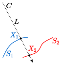
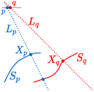
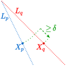
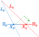
$S_{1}\prec_{L}S_{2}$ (a) surface occlusion	$p\prec q$ (b) pixel occlusion	$p\prec^{0}q$ (c) order-0 occlusion	$p\,{\nprec}\,q\land p\,{\nsucc}\,q$ (d) order-0 wrong occlusion
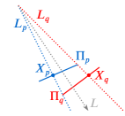
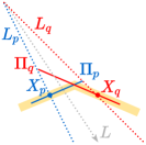
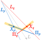
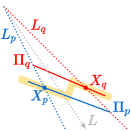
$p\prec^{1}q$ (e) order-1 occlusion	$p\,{\nprec}\,\!^{1}q\land p\,{\nsucc}\,\!^{1}q$ (f) salient angle	$p\,{\nprec}\,\!^{1}q\land p\,{\nsucc}\,\!^{1}q$ (g) reentrant angle	$p\,{\nprec}\,\!^{1}q\land p\,{\nsucc}\,\!^{1}q$ (h) small step

Figure 2: Occlusion configurations (solid lines represent real or tangent surfaces, dotted lines are imaginary lines): (a) $S_{1}$ occludes $S_{2}$ along $L$; (b) $p$ occludes $q$ as $S_{p}$ occludes $S_{q}$ along $L_{p}$; (c) $p$ occludes $q$ at order 0 as $\lVert X_{q}\rVert{-}\lVert X_{p}\rVert\,{\geq}\,\delta\,{>}\,0$, cf. Eq. (1); (d) no occlusion despite order-0 occlusion as $\Pi_{p},\Pi_{q}$ do not occlude one another; (e) $p$ occludes $q$ at order 1 as tangent plane $\Pi_{p}$ occludes tangent plane $\Pi_{q}$ in the $[L_{p},L_{q}]$ cone, cf. Eq. (2); no occlusion for a (f) salient or (g) reentrant angle between tangent planes $\Pi_{p},\Pi_{q}$, cf. Eq. (2); (h) tangent plane occlusion superseded by order-0 non-occlusion, cf. Eq. (2).

2.0.1 Approximating occlusion at order 0.

Given two surface patches $S_{1},S_{2}$ on $\mathcal{S}$ and a ray $L$ (cf. Fig. 2(a)), we say that $S_{1}$ occludes $S_{2}$ along $L$, noted $S_{1}\prec_{L}S_{2}$ (meaning $S_{1}$ comes before $S_{2}$ along $L$), iff $L$ intersects both $S_{1}$ and $S_{2}$, and the intersection $X_{1}=L\cap S_{1}$ is closer to $C$ than $X_{2}=L\cap S_{2}$, i.e., $\lVert X_{1}\rVert<\lVert X_{2}\rVert$.

Now given neighbor pixels $p,q\,{\in}\,\mathcal{P}$, that are also 3D points in the image plane, we say that $p$ occludes $q$, noted $p\prec q$, iff there are surface patches $S_{p},S_{q}$ on $\mathcal{S}$ containing respectively $X_{p},X_{q}$ such that $S_{p}$ occludes $S_{q}$ along $L_{p}$, (cf. Fig. 2(b)). Assuming $L_{p}\,{\cap}\,S_{q}$ exists and $\lVert L_{p}\,{\cap}\,S_{q}\rVert$ can be approximated by $\lVert L_{q}\,{\cap}\,S_{q}\rVert=\lVert X_{q}\rVert$, it leads to a common definition that we qualify as “order-0”. We say that $p$ occludes $q$ at order 0, noted $p\prec^{0}q$ iff $X_{q}$ is deeper than $X_{p}$ (cf. Fig. 2(c)):

$$p\prec^{0}q\text{~{}~{}iff~{}~{}}\lVert X_{p}\rVert<\lVert X_{q}\rVert.$$ (1)

The depth here is w.r.t. the camera center ($d_{p}\,{=}\,\lVert X_{p}\rVert$), not to the image plane. This definition is constructive (can be tested) and the relation is antisymmetric. The case of a minimum margin $\lVert X_{q}\rVert-\lVert X_{p}\rVert\geq\delta>0$ is considered below.

However, when looking at the same continuous surface patch $S_{p}=S_{q}$, the incidence angles of $L_{p},L_{q}$ on $S_{p},S_{q}$ may be such that order-0 occlusion is satisfied whereas there is no actual occlusion, as $S_{q}$ does not pass behind $S_{p}$ (cf. Fig. 2(d)). This yields many false positives, e.g., we observing planar surfaces such as walls.

2.0.2 Approximating occlusion at order 1.

To address this issue, we consider an order-1 approximation of the surface. We assume the scene surface $\mathcal{S}$ is regular enough for a normal $\mathbf{n}_{X}$ to be defined at every point $X$ on $\mathcal{S}$. For any pixel $p$, we consider $\Pi_{p}$ the tangent plane at $X_{p}$ with normal $\mathbf{n}_{p}=\mathbf{n}_{X_{p}}$. Then to assess if $p$ occludes $q$ at order 1, noted $p\prec^{1}q$, we approximate locally $S_{p}$ by $\Pi_{p}$ and $S_{q}$ by $\Pi_{q}$, and study the relative occlusion of $\Pi_{p}$ and $\Pi_{q}$, cf. Fig. 2(d-h).

Looking at a planar surface as in Fig. 2(d), we now have $p{\prec^{0}}q$ as $\lVert X_{p}\rVert\,{<}\,\lVert X_{q}\rVert$, but $p\,{\nprec}\,^{1}q$ because $\Pi_{p}$ does not occlude $\Pi_{q}$, thus defeating the false positive at order 0. A question, however, is on which ray $L$ to test surface occlusion, cf. Fig. 2(a). If we choose $L\,{=}L_{p}$, cf. Fig. 2(b), only $\Pi_{q}$ (approximating $S_{q}$) is actually considered, which is less robust and can lead to inconsistencies due to the asymmetry. If we choose $L=L_{(p+q)/2}$, which passes through an imaginary middle pixel $(p+q)/2$, the formulation is symmetrical but there are issues when $\Pi_{p},\Pi_{q}$ form a sharp edge (salient or reentrant) lying between $L_{p}$ and $L_{q}$, cf. Fig. 2(f-g), which is a common situation in man-made environments. Indeed, the occlusion status then depends on the edge shape and location w.r.t. $L_{(p+q)/2}$, which is little satisfactory. Besides, such declared occlusions are false positives.

To solve this problem, we define order-1 occlusion $p\,{\prec^{1}}q$ as a situation where $\Pi_{p}$ occludes $\Pi_{q}$ along all rays $L$ between $L_{p}$ and $L_{q}$, which can simply be tested as $\lVert X_{p}\rVert\,{<}\,\lVert\Pi_{q}\,{\cap}\,L_{p}\rVert$ and $\lVert X_{q}\rVert\,{>}\,\lVert\Pi_{p}\,{\cap}\,L_{q}\rVert$. However, it raises yet another issue: there are cases where $\lVert X_{p}\rVert\,{<}\,\lVert X_{q}\rVert$, thus $p\,{\prec^{0}}q$, and yet $\lVert\Pi_{p}\,{\cap}\,L\rVert\,{>}\,\lVert\Pi_{q}\,{\cap}\,L\rVert$ for all $L$ between $L_{p}$ and $L_{q}$, implying the inverse occlusion $p\,{\succ^{1}}q$, cf. Fig. 2(h). This small-step configuration exists ubiquitously (e.g., book on a table, frame on a wall) but does not correspond to an actual occlusion. To prevent this paradoxical situation and also to introduce some robustness, as normals can be wrong due to estimation errors, we actually define order-1 occlusion so that it also implies order-0 occlusion. In the end, we say that $p$ occlude $q$ at order 1 iff (i) $p$ occludes $q$ at order 0, (ii) $\Pi_{p}$ occludes $\Pi_{q}$ along all rays $L$ between $L_{p}$ and $L_{q}$, i.e.,

$$p\prec^{1}q\text{~{}~{}iff~{}~{}} \lVert X_{p}\rVert\,{<}\,\lVert X_{q}\rVert~{}\land~{}\lVert X_{p}\rVert\,{<}\,\lVert\Pi_{q}\cap L_{p}\rVert~{}\land~{}\lVert X_{q}\rVert\,{>}\,\lVert\Pi_{p}\cap L_{q}\rVert.$$ (2)

2.0.3 Discretized occlusion.

In practice, we resort to a discrete formulation where $p,q$ are neighboring pixels in image $\mathcal{P}$ and $L_{p}$ passes through the center of $p$. We note $\mathcal{N}_{p}$ the immediate neighbors of $p$, considering either only the 4 horizontal and vertical neighbors $\mathcal{N}_{p}^{4}$, or including also in $\mathcal{N}_{p}^{8}$ the 4 diagonal pixels.

As distances (depths) $d_{p}\,{=}\,\lVert X_{p}\rVert$ can only be measured approximately, we require a minimum discontinuity threshold $\delta\,{>}\,0$ to test any depth difference. A condition $d_{p}\,{<}\,d_{q}$ thus translates as $d_{q}\,{-}\,d_{p}\,{\geq}\,\delta$. However, to treat equally all pairs of neighboring pixels $p,q$, the margin $\delta$ has to be relative to the pixel distance $\lVert p\,{-}\,q\rVert$, which can be $1$ or $\sqrt{2}$ due to the diagonal neighbors. Extending the first-order approximation, the relation $d_{p}\,{<}\,d_{q}$ is thus actually tested as $d_{pq}\,{>}\,\delta$ where $d_{pq}\smash{\,{\stackrel{{\scriptstyle\text{\tiny def}}}{{=}}}\,}(d_{q}-d_{p})/\lVert q-p\rVert$, making $\delta$ a pixel-wise depth increasing rate.

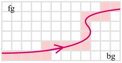
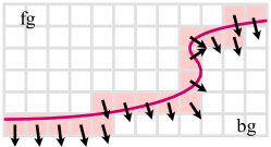
(a) oriented occlusion boundary	(b) oriented occlusion boundary	(c) P2ORM: pixel-pair occlusion
(red curve, fg-on-left convention)	with per-pixel orientation	relation (arrows from occluder to
and boundary rasterization	information (from fg to bg)	occludee, one color per orientation)
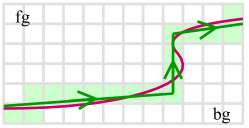
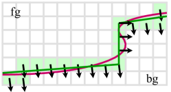
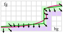
(d) oriented boundary based on	(e) line-segment-based boundary	(f) line-segment-based boundary
annotated line segments (green),	pixels oriented from line orient.	pixels orient. as average direction
yielding a different rasterization	(alt. orientation representation)	of (here) bg neighbors (mauve)
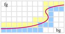
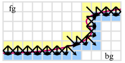
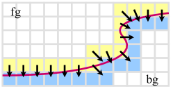
(g) segmentation into layers	(h) fg/bg occlusion relationship:	(i) oriented border pixels (here fg)
with depth ordering, occlusion	with all fg (yellow) $\rightarrow$ bg (blue)	from fg boundary pixel to average
at relative fg/bg pixel boundary	arrows between neighbor pixels	direction of all bg neighbors

Figure 3: Some representations of occlusion and oriented occlusion.

2.0.4 Occlusion relationship and occlusion boundary.

Most of the literature on occlusion in images focuses on occlusion boundaries, that are imaginary lines separating locally a foreground (fg) from a background (bg). A problem is that they are often materialized as rasterized, 1-pixel-wide contours, that are not well defined, cf. Fig. 3(a). The fact is that vectorized occlusion delineations are not generally available in existing datasets, except for handmade annotations, that are coarse as they are made with line segments, with endpoints at discrete positions, only approximating the actual, ideal curve, cf. Fig. 3(d). An alternative representation [42, 17, 53] considers occlusion boundaries at the border pixels of two relative fg/bg segments (regions) rather than on a separating line (Fig. 3(g)).

Inspired by this pixel-border representation but departing from the notion of fg/bg segments, we model occlusion at pixel-level between a fg and a bg pixel, yielding pixel-pair occclusion relationship maps (P2ORM) at image level, cf. Fig. 3(c). An important advantage is that it allows the generation of relatively reliable occlusion information from depth maps, cf. Eq. (2), assuming the depth maps are accurate enough, e.g., generated from synthetic scenes or obtained by high-end depth sensors. Together with photometric data, this occlusion information can then be used as ground truth to train an occlusion relationship estimator from images (see Section 3). Besides, it can model more occlusion configurations, i.e., when a pixel is both occluder and occludee (of different neighbor pixels).

Still, to enable comparison with existing methods, we provide a way to construct traditional boundaries from P2ORM. Boundary-based methods represent occlusion as a mask $(\omega_{p})_{p\in\mathcal{P}}$ such that $\omega_{p}\,{=}\,1$ if pixel $p$ is on an occlusion boundary, and $\omega_{p}\,{=}\,0$ otherwise, with associated predicate $\dot{\omega}_{p}\smash{\,{\stackrel{{\scriptstyle\text{\tiny def}}}{{=}}}\,}(\omega_{p}\,{=}\,1)$. We say that a pixel $p$ is on an occlusion boundary, noted $\dot{\omega}_{p}$, iff it is an occluder or occludee:

$$\dot{\omega}_{p}\text{~{}~{}iff~{}~{}}\exists q\in\mathcal{N}_{p},~{}p\prec q~{}\lor~{}p\succ q.$$ (3)

This defines a 2-pixel-wide boundary, illustrated as the grey region in Fig. 3(c). As we actually estimate occlusion probabilities rather than certain occlusions, this width may be thinned by thresholding or non-maximum suppression (NMS).

2.0.5 Occlusion relationship and oriented occlusion boundary.

Related to the notions of segment-level occlusion relationship, figure/ground representation and boundary ownership [42, 53], occlusion boundaries may be oriented to indicate which side is fg vs bg, cf. Fig. 3(b). It is generally modeled as the direction of the tangent to the boundary, conventionally oriented [17] (fg on the left, Fig. 3(a)). In practice, the boundary is modeled with line segments (Fig. 3(d)), whose orientation $\theta$ is transferred to their rasterized pixels [53] (Fig. 3(e)). Inaccuracies matter little here as the angle is only used to identify a boundary side.

The occlusion border formulation, based on fg/bg pixels (Fig. 3(g)), implicitly captures orientation information: from each fg pixel to each neighbor bg pixel (Fig. 3(h)). So does our modeling (Fig. 3(c)). To compare with boundary-based approaches, we define a notion of pixel occlusion orientation (that could apply to occlusion borders too (Fig. 3(i)), or even boundaries (Fig. 3(f)). We say that a pixel $p$ is oriented as the sum $v_{p}$ of the unitary directions of occluded or occluding neighboring pixels $q$, with angle $\theta_{p}\,{=}\,\operatorname{atan2}(u^{y}_{p},u^{x}_{p})\,{-}\,\frac{\pi}{2}$ where $u_{p}\,{=}\,v_{p}/\lVert v_{p}\rVert$ and

$$v_{p} =\sum_{q\in\mathcal{N}_{p}}(\mathds{1}(p\prec q)-\mathds{1}(p\succ q))\frac{q-p}{\lVert q-p\rVert}.$$ (4)

3 Pixel-pair occlusion relationship estimation

3.0.1 Modeling the pixel-pair occlusion relation.

The occlusion relation is a binary property that is antisymmetric: $p\prec q\Rightarrow q\nprec p$. Hence, to model the occlusion relationship of neighbor pair $pq$, we use a random variable $\omega_{p,q}$ with only three possible values $r\,{\in}\,\{-1,0,1\}$ representing respectively: $p\,{\succ}\,q$ ($p$ is occluded by $q$), $p\,{\nprec}\,q\,{\land}\,\,{p}\,\,{\nsucc}\,q$ (no occlusion between $p$ and $q$), and $p\,{\prec}\,q$ ($p$ occludes $q$).

Since $\omega_{p,q}\,{=}\,{-}\omega_{q,p}$, a single variable per pair is enough. We assume a fixed total ordering $<$ on pixels (e.g., lexicographic order on image coordinates) and note $\omega_{pq}=\omega_{qp}=$ if $p<q$ then $\omega_{p,q}$ else $\omega_{q,p}$. We also define $\omega_{pqr}=\mathbb{P}(\omega_{pq}=r)$.

Concretely, we consider 4 inclinations, horizontal, vertical, diagonal, antidiagonal, with canonical displacements $\mathsf{h}\,{=}\,(1,0)$, $\mathsf{v}\,{=}\,(0,1)$, $\mathsf{d}\,{=}\,(1,1)$, $\mathsf{a}\,{=}\,(1,-1)$, and we call $\mathcal{Q}_{i}\,{=}\,\{pq\,{\mid}\,p,q\,{\in}\,\mathcal{P},q\,{=}\,p\,{+}\,i\}$ the set of pixel pairs with inclination $i\,{\in}\,\mathcal{I}^{4}\,{=}\,\{\mathsf{h},\mathsf{v},\mathsf{d},\mathsf{a}\}$. For the the 4-connectivity, we only consider $i\in\mathcal{I}^{2}\,{=}\,\{\mathsf{h},\mathsf{v}\}$.

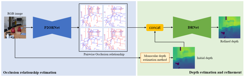
Figure 4: Overview of our method. Left: a encoder-decoder structure followed by softmax takes an RGB image as input and outputs 4 classification maps $(\omega^{i}_{p})$ where each pixel $p$ in a map for inclination $i$ actually represents a pair of pixels $pq$ with $q\,{=}\,p\,{+}\,i$. The map $\omega^{i}_{pq}\,{=}\,\omega^{i}_{p}\,{=}\,r$ classifies $p$ as occluded ($r\,{=}\,{-1}$), not involved in occlusion ($r\,{=}\,0$) or occluding ($r\,{=}\,1$), with probability $\omega^{i}_{pqr}$. (If $\mathcal{N}\,{=}\,\mathcal{N}^{4}$, only 2 inclination maps are generated.) Colors blue, white and red represent respectively $r\,{=}\,{-1}$, $0$ or $1$. The top two images presents occlusion relationships along inclinations horizontal ($i\,{=}\,\mathsf{h}$) and vertical ($i\,{=}\,\mathsf{v}$); the bottom two, along inclinations diagonal ($i\,{=}\,\mathsf{d}$) and antidiagonal ($i\,{=}\,\mathsf{a}$). Right: A direct use of the occlusion relationship for depth map refinement.

3.0.2 Estimating the occlusion relation.

For occlusion relationship estimation, we adopt a segmentation approach: we classify each valid pixel pair $pq$ by scoring its 3 possible statuses $r\,{\in}\,\{-1,0,1\}$, from which we extract estimated probabilities $\hat{\omega}_{pqr}$. The final classification map is obtained as $\hat{\omega}_{pq}=\operatorname*{argmax}_{r}\hat{\omega}_{pqr}$.

Our architecture is sketched on Fig. 4 (left). The P2ORM estimator (named P2ORNet) takes an RGB image as input, and outputs its pixel-pair occlusion relationship map for the different inclinations. We use a ResNet-based [13] U-Net-like auto-encoder with skip-connections [45], cf. supplementary material (SM). It must be noted that this architecture is strikingly simple compared to more complex problem-specific architectures that have been proposed in the past [53, 51, 30]. Besides, our approach is not specifically bound to U-Net or ResNet; in the future, we may benefit from improvements in general segmentation methods.

We train our model with a class-balanced cross-entropy loss [56], taking into account the low probability for a pair $pq$ to be labeled $1$ ($p$ occludes $q$) or $-1$ ($q$ occludes $p$), given that most pixel pairs do not feature any occlusion. Our global loss $\mathcal{L}_{\mathsf{occrel}}$ is a sum of $|\mathcal{I}|$ losses for each kind of pair inclination $i\,{\in}\,\mathcal{I}$, averaged over the number of pairs $|\mathcal{Q}_{i}|$ to balance each task $i\,{\in}\,\mathcal{I}$:

$$\mathcal{L}_{\mathsf{occrel}} =\sum_{i\in\mathcal{I}}\frac{1}{|\mathcal{Q}_{i}|}~{}\;\sum_{\mathclap{\begin{subarray}{c}{pq}\in\mathcal{Q}_{i}\\ r\in\{-1,0,1\}\end{subarray}}}-\alpha_{r}\,\omega_{{pq}r}\log(\hat{\omega}_{{pq}r}).$$ (5)

where $\hat{\omega}_{pqr}$ is the estimated probability that pair $pq$ has occlusion status $r$, $\omega_{pqr}=\mathds{1}(\omega_{pq}\,{=}\,r)$ where $\omega_{pq}$ is the ground truth (GT) occlusion status of pair $pq$, $\alpha_{r}=\mathds{1}(r\,{=}\,0)+\alpha\mathds{1}(r\,{\neq}\,0)$ and $\alpha$ accounts for the disparity in label frequency.

3.0.3 From probabilistic occlusion relations to occlusion boundaries.

As discussed with Eq. (3), occlusion boundaries can be generated from an occlusion relation. In case the relation is available with probabilities, as for an estimated $\hat{\omega}_{pqr}$, we define a probabilistic variant $\omega_{p}\in[0,1]$: $\hat{\omega}_{p}=\frac{1}{|\mathcal{N}_{p}|}\sum_{q\in\mathcal{N}_{p}}(\hat{\omega}_{pq,-1}+\hat{\omega}_{pq,1})$.

As proposed in [6] and performed in many other methods, we operate a non-maximum suppression to get thinner boundaries. The final occlusion boundary map is given by thresholding $\mathrm{NMS}((\omega_{p})_{p\in\mathcal{P}})$ with a probability, e.g., $0.5$.

Boundary orientations can then be generated as defined in Eq. (4). Given our representation, it has the following simpler formulation: $v_{p}=\sum_{q\in\mathcal{N}_{p}}\hat{\omega}_{pq}\frac{q-p}{\lVert q-p\rVert}$.

4 Application to depth map refinement

Given an image, a depth map $(\tilde{d}_{p})_{p\in\mathcal{P}}$ estimated by some method, and an occlusion relationship $(\hat{\omega}_{p,p+i})_{p\in\mathcal{P},i\in\mathcal{I}}$ as estimated in Sect. 3, we produce a refined, more accurate depth map $(d_{p})_{p\in\mathcal{P}}$ with sharper edges. To this end, we propose a U-Net architecture [45] (Fig. 4 (right)), named DRNet, where $(\tilde{d}_{p})_{p\in\mathcal{P}}$ and the 8 maps $((\hat{\omega}_{p,p+i})_{p\in\mathcal{P}})_{i\in\mathcal{I}\cup(-\mathcal{I})}$ are stacked as a multi-channel input of the network.

As a pre-processing, we first use the GT depth map $(d^{\mathsf{gt}}_{p})_{p\in\mathcal{P}}$ and normals $(\mathbf{n}^{\mathsf{gt}}_{p})_{p\in\mathcal{P}}$ to compute the ground-truth occlusion relationship $(p\,{\prec_{\mathsf{gt}}}\,q)_{p\in\mathcal{P},\,q\in\mathcal{N}_{p}}$. We then train the network via the following loss:

$$\mathcal{L}_{\mathsf{refine}} =\mathcal{L}_{\mathsf{occonsist}}+\lambda\mathcal{L}_{\mathsf{regul}}$$ (6)

$$\mathcal{L}_{\mathsf{occonsist}} =\frac{1}{N}\sum_{p\in\mathcal{P}}\ \sum_{q\in\mathcal{N}^{8}_{p}}\left\{\begin{array}[]{ll}\mathcal{B}(\log\delta,\log d_{pq})&\text{~{}if~{}~{}}p\prec_{\mathsf{gt}}q\text{~{}and~{}}d_{pq}<\delta\\ \mathcal{B}(\log\delta,\log D_{pq})&\text{~{}if~{}~{}}p\not\prec_{\mathsf{gt}}q\text{~{}and~{}}D_{pq}\geq\delta\\ 0&\text{~{}otherwise~{}~{}}\\ \end{array}\right.$$ (10)

$$\mathcal{L}_{\mathsf{regul}} =\frac{1}{|\mathcal{P}|}\sum_{p\in\mathcal{P}}\left(\mathcal{B}(\log\tilde{d}_{p},\log{d}_{p})+\lVert\nabla\log\tilde{d}_{p}-\nabla\log{d}_{p}\rVert^{2}\right)$$ (11)

where $\mathcal{B}$ is the berHu loss [22], $\mathcal{\delta}$ is the depth discontinuity threshold introduced in Section 2, $N$ is the number of pixels $p$ having a non-zero contribution to $\mathcal{L}_{\mathsf{occonsist}}$, and $D_{pq}$ is the order-1 depth difference at mid-pixel $(p+q)/2$, i.e., $D_{pq}\,{=}\,\min(d_{pq},m_{pq})$ where $m_{pq}\,{=}\,(\lVert\Pi_{q}\,{\cap}\,L_{(p+q)/2}\rVert{-}\lVert\Pi_{p}\,{\cap}\,L_{(p+q)/2}\rVert)/\lVert q\,{-}\,p\rVert$ is the signed distance between tangent planes $\Pi_{p},\Pi_{q}$ along $L_{(p+q)/2}$.

$\mathcal{L}_{\mathsf{occonsist}}$ penalizes refined depths $d_{p}$ that are inconsistent with GT occlusion relationship $\prec_{\mathsf{gt}}$, i.e., when $p$ occludes $q$ in the GT but not in the refinement, or when $p$ does not occlude $q$ in the GT but does it in the refinement. $\mathcal{L}_{\mathsf{regul}}$ penalizes differences between the rough input depth and the refined output depth, which makes refined depths conditioned on input depths. The total loss $\mathcal{L}_{\mathsf{refine}}$ tends to change depths only close to occlusion boundaries, preventing excessive drifts.

To provide occlusion information that has the same size as the depth map, as pixel-pair information is not perfectly aligned on the pixel grid, we turn pixel-pair data $(\omega_{p,p+i})_{p\in\mathcal{P},i\in\mathcal{I},p{+}i\in\mathcal{P}}$ into a pixelwise information: for a given inclination $i\,{\in}\,\mathcal{I}$, we define $\omega^{i}_{p}=\omega_{p,p+i}$. Thus, e.g., if $p\prec p\,{+}\,i$, then $\omega^{i}_{p}=1$ and $\omega^{i}_{p+i}=-1$.

At test time, given the estimated occlusion relationships, we use NMS to sharpen depth edges. For this, we first generate pixelwise occlusion boundaries from the estimated P2ORM $(\hat{\omega}_{p,p+i})_{p\in\mathcal{P},i\in\mathcal{I}}$, pass them through NMS [6] and do thresholding to get a binary occlusion boundary map $(\omega_{p})_{p\in\mathcal{P}}$ where $\omega_{p}\,{\in}\,\{0,1\}$. We then thin the estimated directional maps $(\omega^{i}_{p})_{p\in\mathcal{P}}$ by setting $\omega^{i}_{p}\leftarrow 0$ if $\omega_{p}\,{=}\,0$.

5 Experiments

Table 1: Used and created occlusion datasets. (a) We only use 500 scenes and 20 images per scene (not all 500M images). (b) Training on NYUv2-OR uses all InteriorNet-OR images adapted using [61] with the 795 training images of NYUv2 as target domain. (c) Training on iBims-1-OR uses all InteriorNet-OR images w/o domain adaptation.

Dataset	InteriorNet-OR	BSDS ownership	NYUv2-OR	iBim-1-OR
Origin	[26]	[42]	[33]	[21]
Type	synthetic	real	real	real
Scene	indoor	outdoor	indoor	indoor
Resolution	640 $\times$ 480	481 $\times$ 321	640 $\times$ 480	640 $\times$ 480
Depth	synthetic	N/A	Kinect v1	laser scanner
Normals	synthetic	N/A	N/A	computed [4]
Relation annot.	ours from depth and normals	ours from manual fig./ground [42]	ours from boundaries and depth	ours from depth and normals
Boundary annot.	from relation	manual [42]	manual [39]	from relation
Orient. annot.	from relation	manual [53]	manual (ours)	from relation
Annot. quality	high	low	medium	high
# train img. (orig.)	10,000(a)	100	795(b)	0(c)
# train images	10,000(a)	100	10,000(b)	10,000(c)
# testing images	0	100	654	100
$\alpha$ in $\mathcal{L}_{\mathsf{occrel}}$	N/A	50	10	10

5.0.1 Oriented occlusion boundary estimation.

Because of the originality of our approach, there is no other method to directly compare with. Yet to demonstrate its significance in task-independent occlusion reasoning, we translate our relation maps into oriented occlusion boundaries (cf. Sect. 3) to compare with SRF-OCC [49], DOC-DMLFOV [53], DOC-HED [53], DOOBNet [51], OFNet [30]${}^{\textrm{1}}$.

To disentangle the respective contributions of the P2ORM formulation and the network architecture, we also evaluate a “baseline” variant of our architecture, that relies on the usual paradigm of estimating separately boundaries and orientations [53, 51, 30]: we replace the last layer of our pixel-pair classifier by two separate heads, one for classifying the boundary and the other one for regressing the orientation, and we use the same loss as [51, 30].

We evaluate on 3 datasets: BSDS ownership [42], NYUv2-OR, iBims-1-OR (cf. Tab. 1). We keep the original training and testing data of BSDS. NYUv2-OR is tested on a subset of NYUv2 [33] with occlusion boundaries from [39] and our labeled orientation. iBims-1-OR is tested on iBims-1 [21] augmented with occlusion ground truth we generated automatically (cf. Sect. 2 and SM). As illustrated on Fig. 5, this new accurate ground truth is much more complete than the “distinct depth transitions” offered by iBims-1 [21], that are first detected on depth maps with [6], then manually selected. For training, a subset of InteriorNet [26] is used for NYUv2-OR and iBims-1-OR. For NYUv2-OR, because of the domain gap between sharp InteriorNet images and blurry NYUv2 images, the InteriorNet images are furthermore adapted with [61] using NYUv2 training images (see SM for the ablation study related to domain adaption).

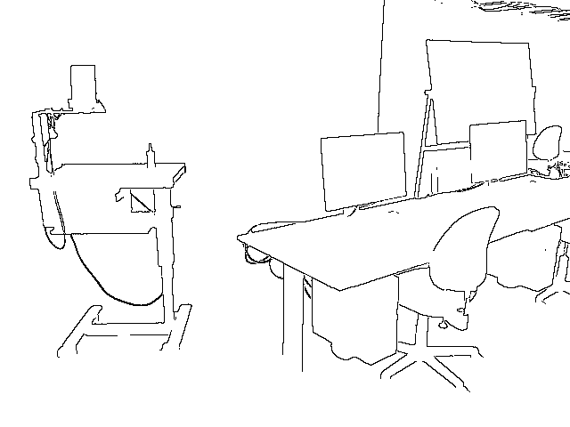
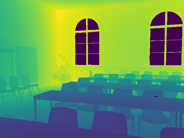
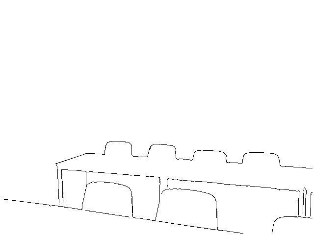
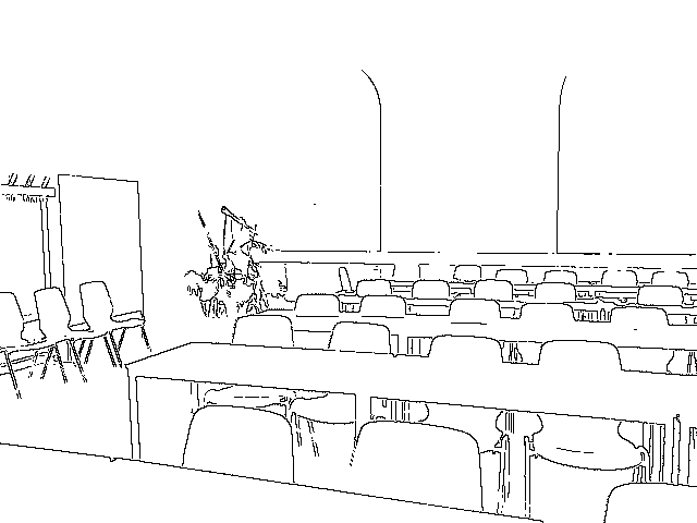
(a)	(b)	(c)	(d)

Figure 5: iBims-1-OR: (a) RGB images, (b) GT depth (invalid is black), (c) provided “distinct depth transitions” [21], (d) our finer and more complete occlusion boundaries.

We use the same protocol as [51, 30] to compute 3 standard evaluation metrics, based on the Occlusion-Precision-Recall graph (OPR): F-measure with best fixed occlusion probability threshold over the all dataset (ODS), F-measure with best occlusion probability threshold for each image (OIS), and average precision over all occlusion probability thresholds (AP). Recall (R) is the proportion of correct boundary detections, while Precision (P) is the proportion of pixels with correct occlusion orientation w.r.t. all pixels detected as occlusion boundary.

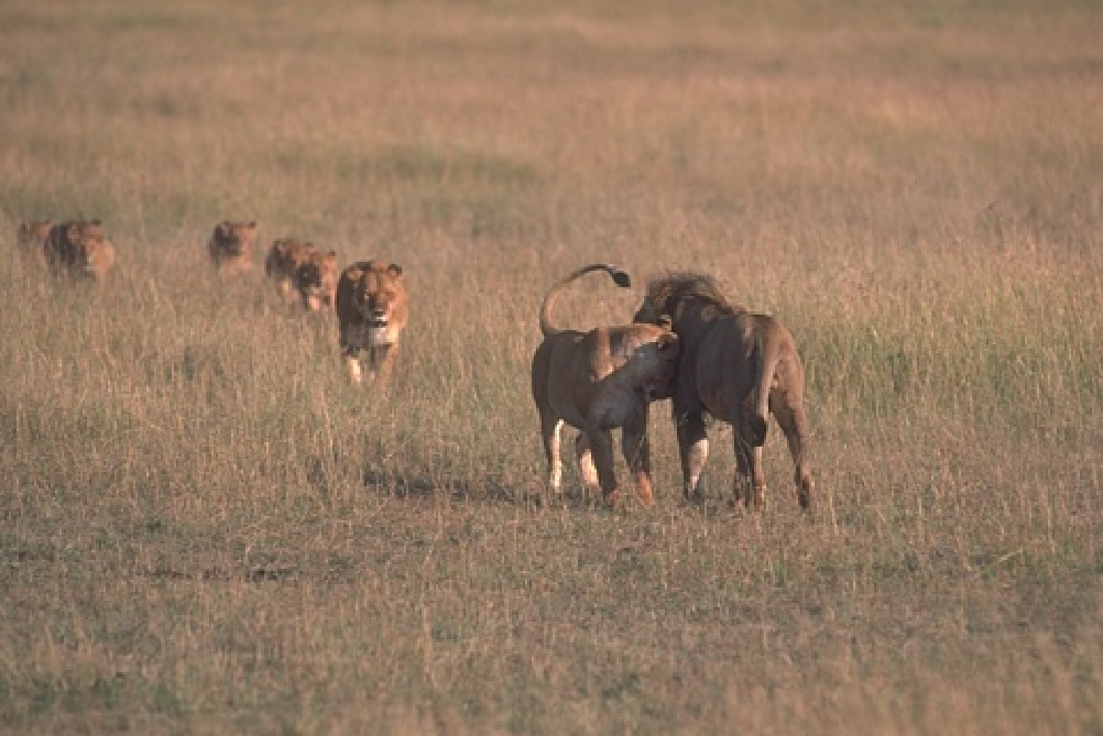
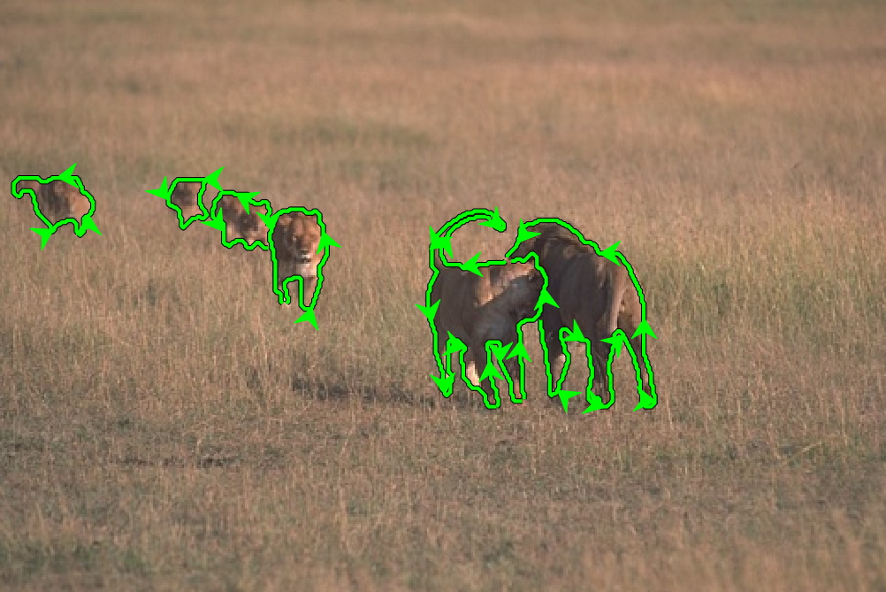
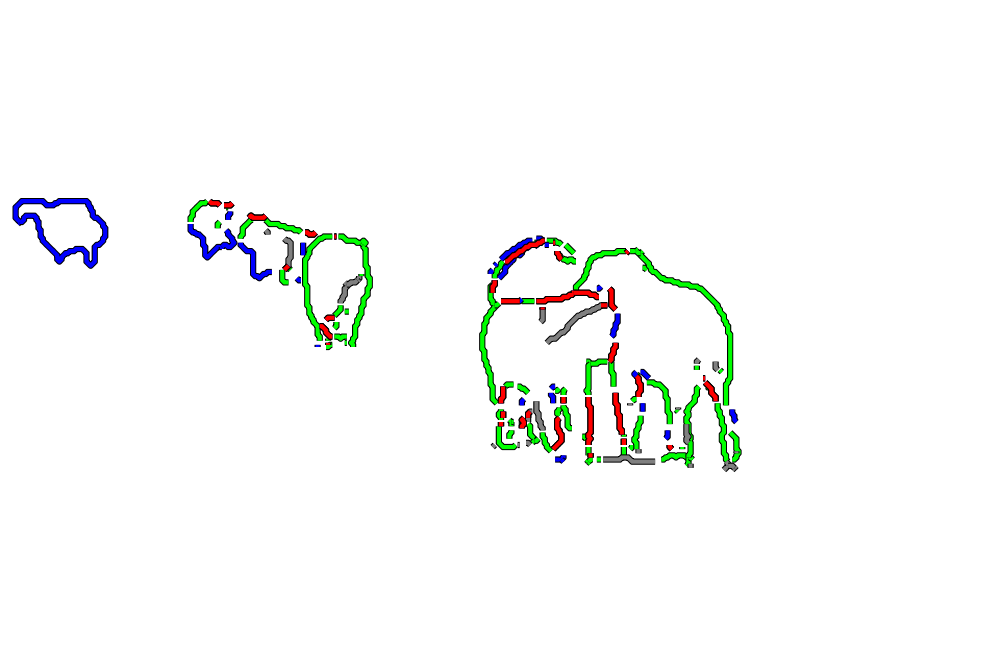
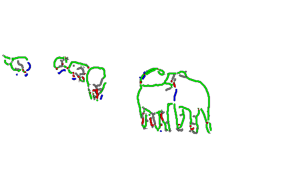
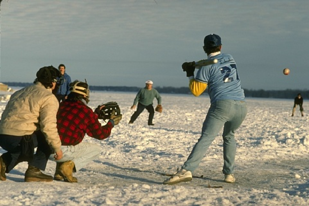
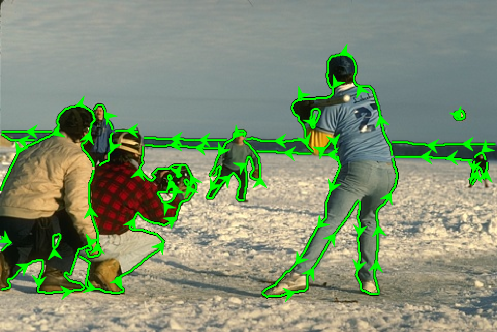
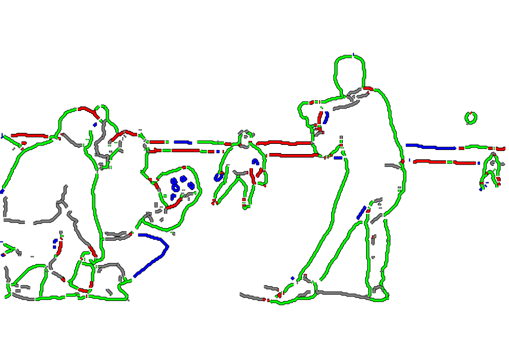
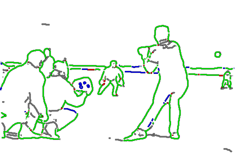
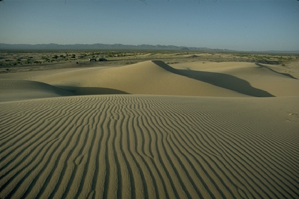
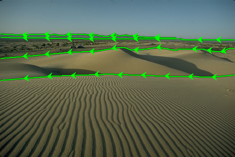
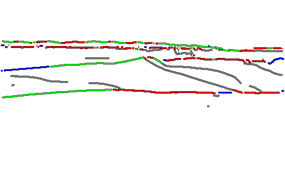
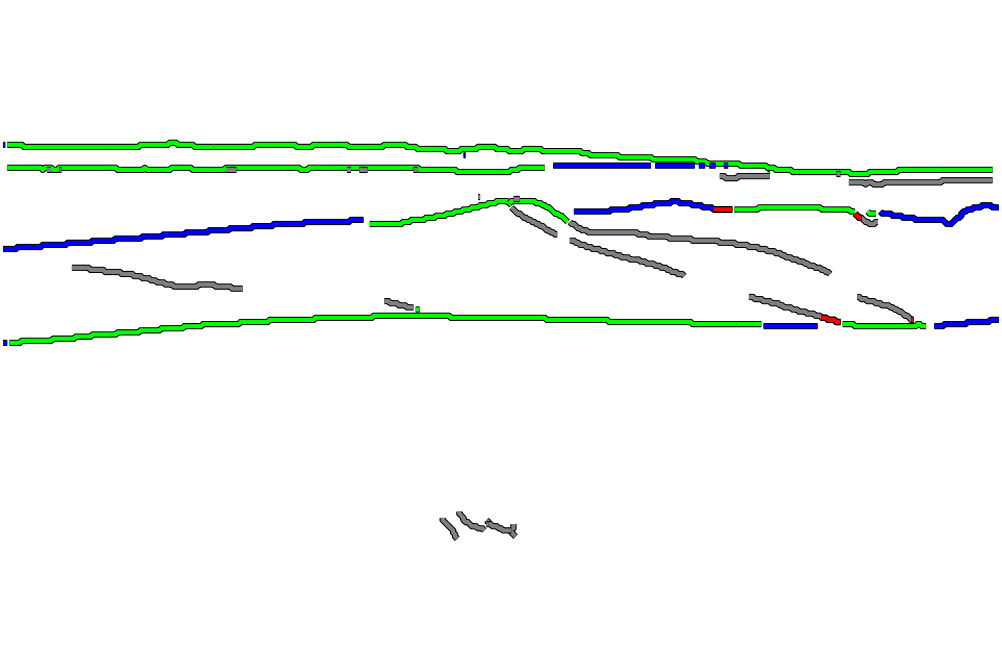
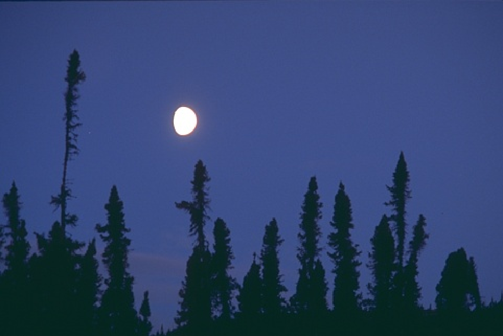
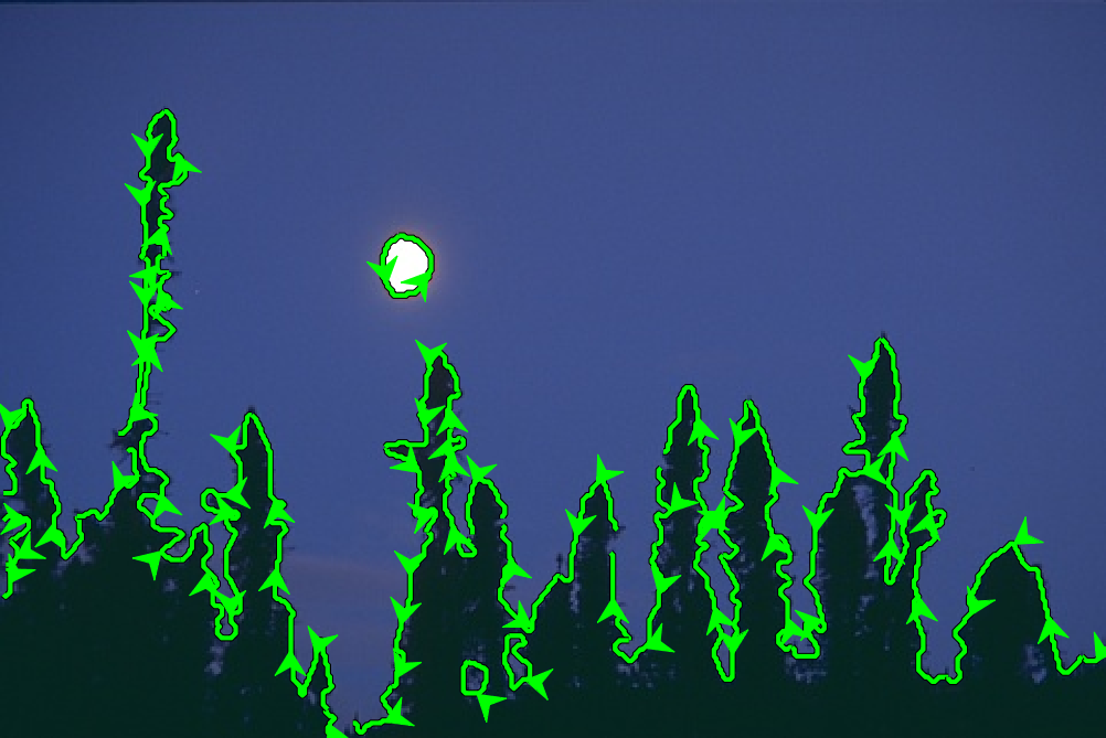
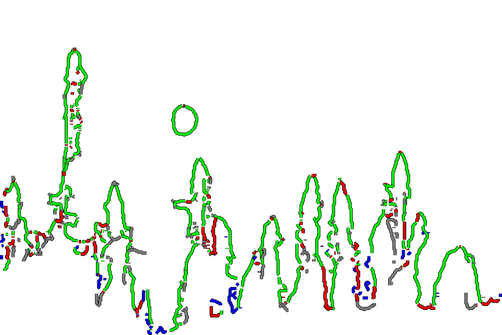
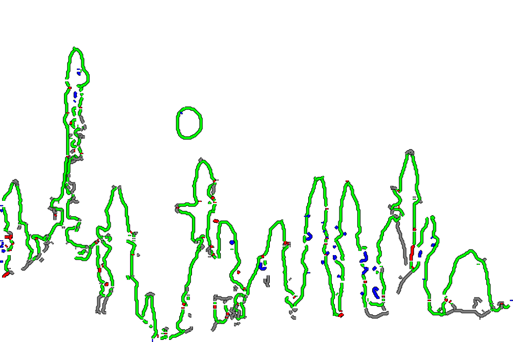
(a)	(b)	(c)	(d)

Figure 6: Occlusion estimation on BSDS ownership dataset: (a) input RGB image, (b) ground-truth occlusion orientation, (c) OFNet estimation [30], (d) our estimation. green: correct boundary and orientation; red: correct boundary, incorrect orientation; blue: missed boundaries; gray: incorrect boundaries.

Table 2: Oriented occlusion boundary estimation. *Our re-implementation.

Method	BSDS ownership			NYUv2-OR			iBims-1-OR
Metric	ODS	OIS	AP	ODS	OIS	AP	ODS	OIS	AP
SRF-OCC [49]	.419	.448	.337	-	-	-	-	-	-
DOC-DMLFOV [53]	.463	.491	.369	-	-	-	-	-	-
DOC-HED [53]	.522	.545	.428	-	-	-	-	-	-
DOOBNet [51]	.555	.570	.440	-	-	-	-	-	-
OFNet [30]	.583	.607	.501	-	-	-	-	-	-
DOOBNet*	.529	.543	.433	.343	.370	.263	.421	.440	312
OFNet*	.553	.577	.520	.402	.431	.342	.488	.513	.432
baseline	.571	.605	.524	.396	.428	.343	.482	.507	.431
ours (4-connectivity)	.590	.612	.512	.500	.522	.477	.575	.599	.508
ours (8-connectivity)	.607	.632	.598	.520	.540	.497	.581	.603	.525

Qualitative results are shown in Fig. 6, while Table 2 summarizes quantitative results. Our baseline is on par with the state-of-the-art on the standard BSDS ownership benchmark as well as on the two new datasets, hinting that complex specific architectures maybe buy little as a common ResNet-based U-Net is at least as efficient. More importantly, our method with 8-connectivity outperforms existing methods on all metrics by a large margin (up to 15 points), demonstrating the significance of our formulation on higher-quality annotations, as opposed to BSDS whose lower quality levels up performances. It could also be an illustration that classification is often superior to regression [32] as it does not average ambiguities. Lastly, the 4-connectivity variant shows that the ablation of diagonal neighbors decreases the performance, thus assessing the relevance of 8-connectivity. (See SM for more results and ablation studies.)

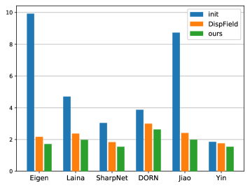
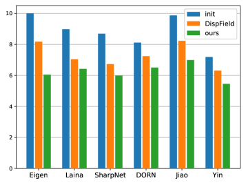
NYUv2	$\epsilon_{\textit{acc}}$	$\epsilon_{\textit{comp}}$
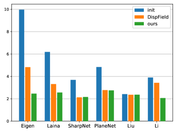
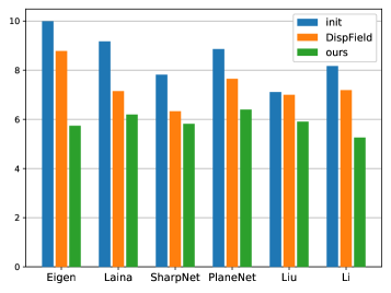
iBims-1	$\epsilon_{\textit{acc}}$	$\epsilon_{\textit{comp}}$

Figure 7: Gain in edge quality after depth refinement for metrics $\epsilon_{\textit{acc}}$ (left) and $\epsilon_{\textit{comp}}$ (right) on NYUv2 (top) for respectively [8, 22, 40, 9, 20, 58] and on iBimis-1 (bottom) for [8, 22, 40, 27, 28, 25]: metric on input depth maps (blue), after refining with [39] (orange), and after our refinement (green). Lower metric value is better.

5.0.2 Depth map refinement.

To assess our refinement approach, we compare with [39], which is the current state-of-the-art for depth refinement on boundaries.

We evaluate based on depth maps estimated by methods that offer results on depth-edge metrics: [8, 22, 9, 40, 20, 58] on NYUv2, and [8, 28, 25, 22, 40, 27] on iBims-1. We train our network on InteriorNet-OR for ground truth, with input depth maps to refine estimated by SharpNet [40]. For a fair comparison, we follow the evaluation protocol of [39]. To assess general depth accuracy, we measure: mean absolute relative error (rel), mean $\log_{10}$ error ($\log_{10}$), Root Mean Squared linear Error (RMSE(lin)), Root Mean Squared log Error (RMSE(log)), and accuracy under threshold ($\sigma_{i}\,{<}\,1.25^{i})_{i=1,2,3}$. For depth-edge, following [21], we measure the accuracy $\epsilon_{\textit{acc}}$ and completion $\epsilon_{\textit{comp}}$ of predicted boundaries.

Fig. 7 summarizes quantitative results. We significantly improve edge metrics $\epsilon_{\textit{acc}},\epsilon_{\textit{comp}}$ on NYUv2 and iBims-1, systematically outperforming [39] and showing consistency across the two different datasets. Not shown on the figure (see SM), the differences on general metrics after refinement are negligible ($<$ 1%), i.e., we improve sharpness without degrading the overall depth. Fig. 8 illustrates the refinement on depth maps estimated by SharpNet [40]. We also outperform many methods based on image intensity [50, 12, 3, 55, 47] (see SM), showing the superiority of P2ORM for depth refinement w.r.t. image intensity.

In an extensive variant study (see SM), we experiment with possible alternatives: adding as input in the architecture (1) the original image, (2) the normal map, (3) the binary edges; (4) adding an extra loss term $\mathcal{L}_{\mathsf{gtdepth}}$ that regularizes on the ground truth depths rather than on the estimated depth, or substituting $\mathcal{L}_{\mathsf{gtdepth}}$ (5) for $\mathcal{L}_{\mathsf{occonsist}}$ or (6) for $\mathcal{L}_{\mathsf{regul}}$; using (7) $d_{pq}$ only, or (8) $D_{pq}$ only in Eq. (11). The alternative proposed here performs the best.

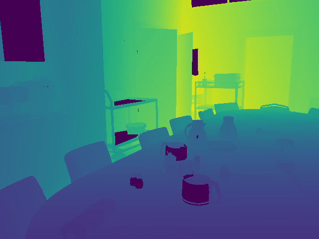
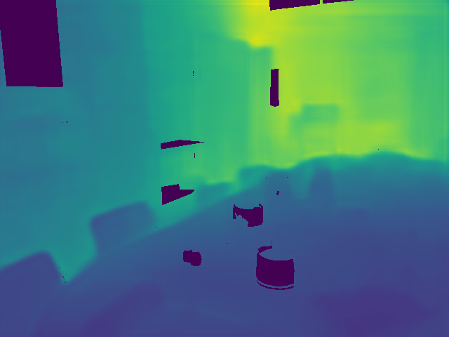
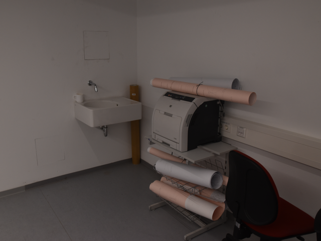
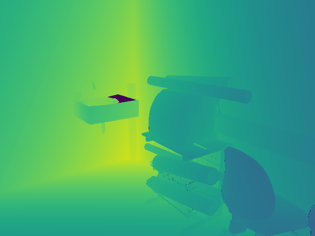
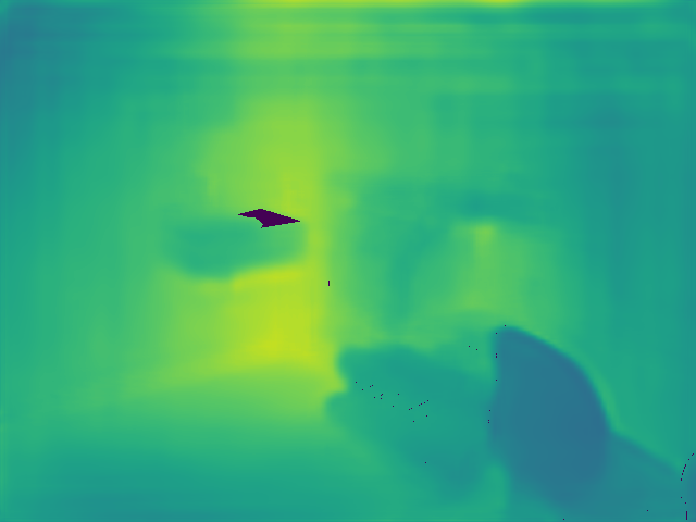
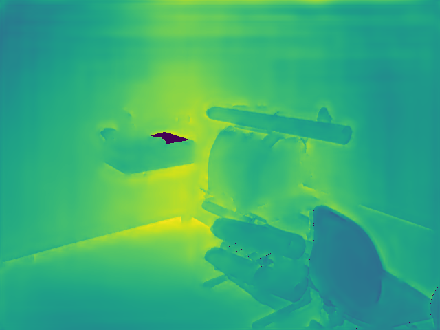
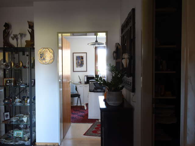
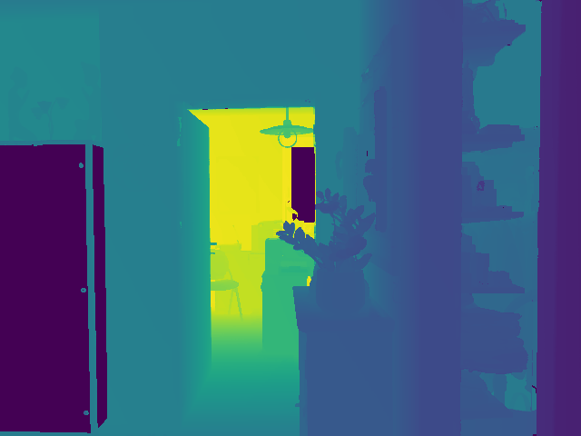
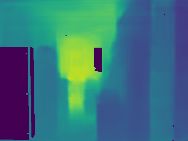
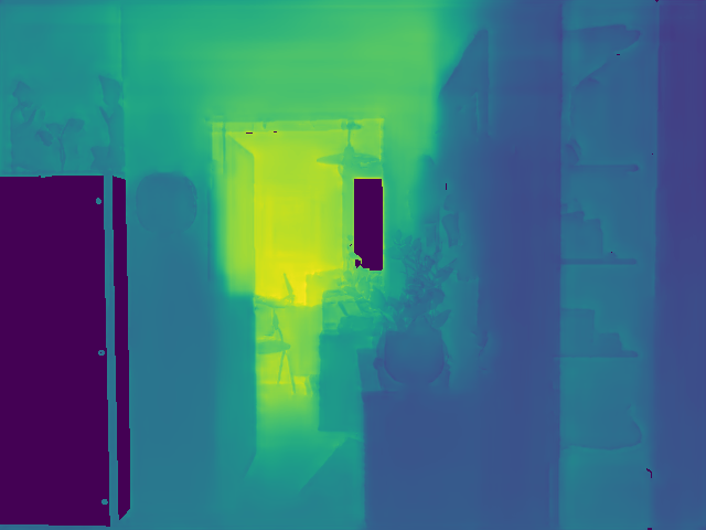
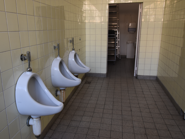
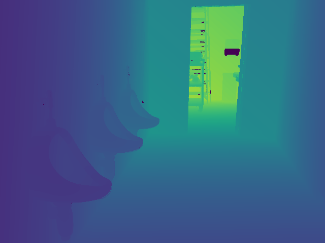
(a)	(b)	(c)	(d)

Figure 8: Depth refinement: (a) input RGB image from iBims-1, (b) ground truth depth, (c) SharpNet depth prediction [40], (d) our refined depth.

6 Conclusion

In this paper, we propose a new representation of occlusion relationship based on pixel pairs and design a simple network architecture to estimate it. Translating our results into standard occlusion boundaries for comparison, we significantly outperform the state-of-the-art for both occlusion boundary and oriented occlusion boundary estimation. To illustrate the potential of our representation, we also propose a depth map refinement model that exploits our estimated occlusion relationships. It also consistently outperforms the state-of-the-art regarding depth edge sharpness, without degrading accuracy in the rest of the depth image. These results are made possible thanks to a new method to automatically generate accurate occlusion relationship labels from depth maps, at a large scale.

Acknowledgements.

We thank Yuming Du and Michael Ramamonjisoa for helpful discussions and for offering their GT annotations of occlusion boundaries for a large part of NYUv2, which we completed (NYUv2-OC++) [39]. This work was partly funded by the I-Site FUTURE initiative, through the DiXite project.

References

- [1] Acuna, D., Kar, A., Fidler, S.: Devil is in the edges: Learning semantic boundaries from noisy annotations. In: Conference on Computer Vision and Pattern Recognition (CVPR). pp. 11075–11083 (2019)
- [2] Apostoloff, N., Fitzgibbon, A.: Learning spatiotemporal t-junctions for occlusion detection. In: Conference on Computer Vision and Pattern Recognition (CVPR). vol. 2, pp. 553–559. IEEE (2005)
- [3] Barron, J.T., Poole, B.: The fast bilateral solver. In: European Conference on Computer Vision (ECCV). pp. 617–632 (2016)
- [4] Boulch, A., Marlet, R.: Fast and robust normal estimation for point clouds with sharp features. Computer Graphics Forum (CGF) 31(5), 1765–1774 (2012)
- [5] Cooper, M.C.: Interpreting line drawings of curved objects with tangential edges and surfaces. Image and Vision Computing 15(4), 263–276 (1997)
- [6] Dollár, P., Zitnick, C.L.: Fast edge detection using structured forests. IEEE Transactions on Pattern analysis and Machine Intelligence (PAMI) 37(8), 1558–1570 (2014)
- [7] Eigen, D., Fergus, R.: Predicting depth, surface normals and semantic labels with a common multi-scale convolutional architecture. In: Conference on Computer Vision and Pattern Recognition (CVPR). pp. 2650–2658 (2015)
- [8] Eigen, D., Puhrsch, C., Fergus, R.: Depth map prediction from a single image using a multi-scale deep network. In: Ghahramani, Z., Welling, M., Cortes, C., Lawrence, N.D., Weinberger, K.Q. (eds.) Advances in Neural Information Processing Systems (NeurIPS), pp. 2366–2374. Curran Associates, Inc. (2014)
- [9] Fu, H., Gong, M., Wang, C., Batmanghelich, K., Tao, D.: Deep ordinal regression network for monocular depth estimation. In: Conference on Computer Vision and Pattern Recognition (CVPR). pp. 2002–2011 (2018)
- [10] Fu, H., Wang, C., Tao, D., Black, M.J.: Occlusion boundary detection via deep exploration of context. In: Conference on Computer Vision and Pattern Recognition (CVPR). pp. 241–250 (2016)
- [11] Godard, C., Mac Aodha, O., Brostow, G.J.: Unsupervised monocular depth estimation with left-right consistency. In: Conference on Computer Vision and Pattern Recognition (CVPR). pp. 270–279 (2017)
- [12] He, K., Sun, J., Tang, X.: Guided image filtering. In: European Conference on Computer Vision (ECCV). pp. 1–14 (2010)
- [13] He, K., Zhang, X., Ren, S., Sun, J.: Deep residual learning for image recognition. In: Conference on Computer Vision and Pattern Recognition (CVPR). pp. 770–778 (2016)
- [14] He, X., Yuille, A.: Occlusion boundary detection using pseudo-depth. In: European Conference on Computer Vision (ECCV). pp. 539–552. Springer (2010)
- [15] Heise, P., Klose, S., Jensen, B., Knoll, A.: PM-Huber: Patchmatch with Huber regularization for stereo matching. In: International Conference on Computer Vision (ICCV). pp. 2360–2367 (2013)
- [16] Heo, M., Lee, J., Kim, K.R., Kim, H.U., Kim, C.S.: Monocular depth estimation using whole strip masking and reliability-based refinement. In: European Conference on Computer Vision (ECCV). pp. 36–51 (2018)
- [17] Hoiem, D., Efros, A.A., Hebert, M.: Recovering occlusion boundaries from an image. International Journal of Computer Vision (IJCV) 91, 328–346 (2010)
- [18] Hong, Z., Chen, Z., Wang, C., Mei, X., Prokhorov, D., Tao, D.: Multi-store tracker (muster): A cognitive psychology inspired approach to object tracking. In: Conference on Computer Vision and Pattern Recognition (CVPR). pp. 749–758 (2015)
- [19] Ilg, E., Saikia, T., Keuper, M., Brox, T.: Occlusions, motion and depth boundaries with a generic network for disparity, optical flow or scene flow estimation. In: European Conference on Computer Vision (ECCV). pp. 614–630 (2018)
- [20] Jiao, J., Cao, Y., Song, Y., Lau, R.W.H.: Look deeper into depth: Monocular depth estimation with semantic booster and attention-driven loss. In: European Conference on Computer Vision (ECCV) (2018)
- [21] Koch, T., Liebel, L., Fraundorfer, F., Körner, M.: Evaluation of CNN-based single-image depth estimation methods. In: Leal-Taixé, L., Roth, S. (eds.) European Conference on Computer Vision Workshops (ECCV Workshops). pp. 331–348. Springer International Publishing (2019)
- [22] Laina, I., Rupprecht, C., Belagiannis, V., Tombari, F., Navab, N.: Deeper depth prediction with fully convolutional residual networks. In: International Conference on 3D Vision (3DV). pp. 239–248. IEEE (2016)
- [23] Lee, J.H., Kim, C.S.: Monocular depth estimation using relative depth maps. In: Conference on Computer Vision and Pattern Recognition (CVPR). pp. 9729–9738 (2019)
- [24] Leichter, I., Lindenbaum, M.: Boundary ownership by lifting to 2.1-D. In: International Conference on Computer Vision (ICCV). pp. 9–16. IEEE (2008)
- [25] Li, J.Y., Klein, R., Yao, A.: A two-streamed network for estimating fine-scaled depth maps from single RGB images. In: International Conference on Computer Vision (ICCV). pp. 3392–3400 (2016)
- [26] Li, W., Saeedi, S., McCormac, J., Clark, R., Tzoumanikas, D., Ye, Q., Huang, Y., Tang, R., Leutenegger, S.: InteriorNet: Mega-scale multi-sensor photo-realistic indoor scenes dataset. In: British Machine Vision Conference (BMVC) (2018)
- [27] Liu, C., Yang, J., Ceylan, D., Yumer, E., Furukawa, Y.: PlaneNet: Piece-wise planar reconstruction from a single RGB image. In: Conference on Computer Vision and Pattern Recognition (CVPR). pp. 2579–2588 (2018)
- [28] Liu, F., Shen, C., Lin, G.: Deep convolutional neural fields for depth estimation from a single image. In: Conference on Computer Vision and Pattern Recognition (CVPR) (2015)
- [29] Liu, Y., Cheng, M.M., Fan, D.P., Zhang, L., Bian, J., Tao, D.: Semantic edge detection with diverse deep supervision. arXiv preprint arXiv:1804.02864 (2018)
- [30] Lu, R., Xue, F., Zhou, M., Ming, A., Zhou, Y.: Occlusion-shared and feature-separated network for occlusion relationship reasoning. In: International Conference on Computer Vision (ICCV) (2019)
- [31] Martin, D.R., Fowlkes, C.C., Malik, J.: Learning to detect natural image boundaries using local brightness, color, and texture cues. IEEE Transactions on Pattern analysis and Machine Intelligence (PAMI) 26(5), 530–549 (2004)
- [32] Massa, F., Marlet, R., Aubry, M.: Crafting a multi-task CNN for viewpoint estimation. In: British Machine Vision Conference (BMVC) (2016)
- [33] Nathan Silberman, Derek Hoiem, P.K., Fergus, R.: Indoor segmentation and support inference from RGBD images. In: European Conference on Computer Vision (ECCV) (2012)
- [34] Nitzberg, M., Mumford, D.B.: The 2.1-D sketch. IEEE Computer Society Press (1990)
- [35] Oberweger, M., Rad, M., Lepetit, V.: Making deep heatmaps robust to partial occlusions for 3D object pose estimation. In: European Conference on Computer Vision (ECCV). pp. 119–134 (2018)
- [36] Peng, S., Liu, Y., Huang, Q., Zhou, X., Bao, H.: PVNet: Pixel-wise voting network for 6DoF pose estimation. In: Conference on Computer Vision and Pattern Recognition (CVPR). pp. 4561–4570 (2019)
- [37] Rad, M., Lepetit, V.: BB8: A scalable, accurate, robust to partial occlusion method for predicting the 3D poses of challenging objects without using depth. In: International Conference on Computer Vision (ICCV). pp. 3828–3836 (2017)
- [38] Rafi, U., Gall, J., Leibe, B.: A semantic occlusion model for human pose estimation from a single depth image. In: Conference on Computer Vision and Pattern Recognition Workshops (CVPR Workshops). pp. 67–74 (2015)
- [39] Ramamonjisoa, M., Du, Y., Lepetit, V.: Predicting sharp and accurate occlusion boundaries in monocular depth estimation using displacement fields. In: Conference on Computer Vision and Pattern Recognition (CVPR). pp. 14648–14657 (2020)
- [40] Ramamonjisoa, M., Lepetit, V.: Sharpnet: Fast and accurate recovery of occluding contours in monocular depth estimation. In: International Conference on Computer Vision Workshops (ICCV Workshops) (2019)
- [41] Raskar, R., Tan, K.H., Feris, R., Yu, J., Turk, M.: Non-photorealistic camera: depth edge detection and stylized rendering using multi-flash imaging. ACM Transactions on Graphics (TOG) 23(3), 679–688 (2004)
- [42] Ren, X., Fowlkes, C.C., Malik, J.: Figure/ground assignment in natural images. In: European Conference on Computer Vision (ECCV). pp. 614–627. Springer (2006)
- [43] Ricci, E., Ouyang, W., Wang, X., Sebe, N., et al.: Monocular depth estimation using multi-scale continuous CRFs as sequential deep networks. IEEE Transactions on Pattern analysis and Machine Intelligence (PAMI) 41(6), 1426–1440 (2018)
- [44] Roberts, L.G.: Machine perception of three-dimensional solids. Ph.D. thesis, Massachusetts Institute of Technology (1963)
- [45] Ronneberger, O., Fischer, P., Brox, T.: U-Net: Convolutional networks for biomedical image segmentation. In: International Conference on Medical Image Computing & Computer Assisted Intervention (MICCAI) (2015)
- [46] Stein, A.N., Hebert, M.: Occlusion boundaries from motion: Low-level detection and mid-level reasoning. International Journal of Computer Vision (IJCV) 82, 325–357 (2008)
- [47] Su, H., Jampani, V., Sun, D., Gallo, O., Learned-Miller, E., Kautz, J.: Pixel-adaptive convolutional neural networks. In: Conference on Computer Vision and Pattern Recognition (CVPR). pp. 11166–11175 (2019)
- [48] Sugihara, K.: Machine interpretation of line drawings, vol. 1. MIT press Cambridge (1986)
- [49] Teo, C., Fermuller, C., Aloimonos, Y.: Fast 2D border ownership assignment. In: Conference on Computer Vision and Pattern Recognition (CVPR). pp. 5117–5125 (2015)
- [50] Tomasi, C., Manduchi, R.: Bilateral filtering for gray and color images. In: International Conference on Computer Vision (ICCV). pp. 839–846 (1998)
- [51] Wang, G., Liang, X., Li, F.W.B.: DOOBNet: Deep object occlusion boundary detection from an image. In: Asian Conference on Computer Vision (ACCV) (2018)
- [52] Wang, P., Shen, X., Russell, B., Cohen, S., Price, B., Yuille, A.L.: Surge: Surface regularized geometry estimation from a single image. In: Advances in Neural Information Processing Systems (NeurIPS). pp. 172–180 (2016)
- [53] Wang, P., Yuille, A.: DOC: Deep occlusion estimation from a single image. In: European Conference on Computer Vision (ECCV) (2016)
- [54] Wang, Y., Yang, Y., Yang, Z., Zhao, L., Wang, P., Xu, W.: Occlusion aware unsupervised learning of optical flow. In: Conference on Computer Vision and Pattern Recognition (CVPR). pp. 4884–4893 (2018)
- [55] Wu, H., Zheng, S., Zhang, J., Huang, K.: Fast end-to-end trainable guided filter. In: Conference on Computer Vision and Pattern Recognition (CVPR). pp. 1838–1847 (2018)
- [56] Xie, S., Tu, Z.: Holistically-nested edge detection. In: International Conference on Computer Vision (ICCV). pp. 1395–1403 (2015)
- [57] Xu, D., Ricci, E., Ouyang, W., Wang, X., Sebe, N.: Multi-scale continuous CRFs as sequential deep networks for monocular depth estimation. In: Conference on Computer Vision and Pattern Recognition (CVPR). pp. 5354–5362 (2017)
- [58] Yin, W., Liu, Y., Shen, C., Yan, Y.: Enforcing geometric constraints of virtual normal for depth prediction. In: International Conference on Computer Vision (ICCV) (2019)
- [59] Yu, Z., Feng, C., Liu, M.Y., Ramalingam, S.: CASENet: Deep category-aware semantic edge detection. In: Conference on Computer Vision and Pattern Recognition (CVPR). pp. 5964–5973 (2017)
- [60] Yu, Z., Liu, W., Zou, Y., Feng, C., Ramalingam, S., Vijaya Kumar, B., Kautz, J.: Simultaneous edge alignment and learning. In: European Conference on Computer Vision (ECCV). pp. 388–404 (2018)
- [61] Zheng, C., Cham, T.J., Cai, J.: T2Net: Synthetic-to-realistic translation for solving single-image depth estimation tasks. In: European Conference on Computer Vision (ECCV). pp. 767–783 (2018)
- [62] Zitnick, C.L., Kanade, T.: A cooperative algorithm for stereo matching and occlusion detection. IEEE Transactions on Pattern analysis and Machine Intelligence (PAMI) 22(7), 675–684 (2000)