Blocked populations in ring-shaped optical lattices

Abstract

We study a special dynamical regime of a Bose-Einstein condensate in a ring-shaped lattice where the populations in each site remain constant during the time evolution. The states in this regime are characterized by equal occupation numbers in alternate wells and non-trivial phases, while the phase differences between neighboring sites evolve in time yielding persistent currents that oscillate around the lattice. We show that the velocity circulation around the ring lattice alternates between two values determined by the number of wells and with a specific time period that is only driven by the onsite interaction energy parameter. In contrast to the self-trapping regime present in optical lattices, the occupation number at each site does not show any oscillation and the particle imbalance does not possess a lower bound for the phenomenon to occur. These findings are predicted with a multimode model and confirmed by full three-dimensional Gross-Pitaevskii simulations using an effective onsite interaction energy parameter.

I Introduction

The self-trapping phenomenon has been extensively studied in double-well systems by means of a two-mode model smerzi97 , ragh99 , anan06 , jia08 , mele11 , abad11 , mauro17 , doublewell , and experimentally observed by Albiez et al. albiez05 , thesisAlbiez , thesisGati . In this regime the population in one site remains higher than the one in the other well over all the evolution. This imbalance of particles performs oscillations around the non vanishing mean value, whereas the phase difference between the sites exhibits a running phase behavior. Theoretical studies of this phenomenon has been also carried out by several authors in extended regular lattices Anker2005 , Wang2006 , optlat , stlastoplat . More recently, the study of self-trapping has also been addressed in ring-shaped optical lattices cuatropozos06 , arwas2014 , mauro4p . Such works treat three- and four-well systems. In Refs. cuatropozos06 , arwas2014 the dynamics has been investigated through a multimode (M) model that utilized ad-hoc values for the hopping and onsite energy parameters. Whereas in Ref. mauro4p , such parameters have been extracted from a mean-field approach using three-dimensional localized “Wannier-like” (WL) onsite functions and including an effective onsite interaction energy parameter jezek13a , jezek13b . For large filling numbers, the inclusion of such a realistic interaction parameter has been shown to be crucial for the accurate description of the dynamics, yielding a sizable change on the time periods respect to those obtained by the standard model. In contrast, for filling number around unity mean-field approaches are not applicable and hence other microscopic methods have to be used Kolovski2006 , Gallemi2016 . In Ref. Burchianti2017 , it has been demonstrated that an effective interaction can also be extracted from the Bogoliubov excitations in the case of the Josephson regime. A systematic study of the self-trapping regime and the crossover to the Josephson oscillations in four-well systems including non-symmetric configurations has been developed in Ref. mauro4p . It is worthwhile noticing that the dynamics in multiple well condensates constitutes a promising area provided that successful efforts have been performed to experimentally construct ring-shaped optical lattices hen09 .

In this work we demonstrate theoretically the existence of a dynamical regime that exhibits a novel behavior. If the number of wells of the lattice is a multiple of four, there exists a family of nonstationary states with constant site populations and special non-trivial phases. These states could be regarded as a special variation of a ST regime where, in contrast to that observed in two- and multiple-well condensates smerzi97 , ragh99 , mauro17 , mauro4p , the population imbalance between neighboring sites can be arbitrarily low and do not exhibit any oscillation in time. For such states the M model order parameter can be expressed as a linear combination of particular degenerate Gross-Pitaevskii (GP) stationary states. However, due to the nonlinear nature of the GP equation, the states are nonstationary. The dynamics of these states is governed only by the onsite interaction energy parameter. We explicitly show that the angular momentum exhibits a simple oscillating behavior and that the velocity circulation around the ring alternates periodically between values $-N_{c}/4$ and $N_{c}/4$, being $N_{c}$ the number of weakly linked condensates. A goal of this work is to obtain an analytical expression for such a time period which involves only the imbalance and the effective interaction parameter. By comparing the evolution of the phase differences obtained through GP simulations for a four-well system and with the M model, we can establish the accuracy of such a parameter. The existence of these states is confirmed numerically by means of full three-dimensional Gross-Pitaevskii (GP) simulations showing a perfect accordance to the M model predictions for several population imbalances. Furthermore, a Floquet stability analysis confirms that for the imbalances studied here the dynamics turns out to be regular.

The paper is organized as follows. In Sec. II we briefly review the main concepts of the multimode model. In particular, we rewrite the equations of motion which include an effective onsite interaction parameter mauro4p and we outline the construction of the localized states in terms of the GP stationary ones. In Sec. III we describe the specific four-well system used in the numerical simulations. Section IV is devoted to study the properties of these states with blocked occupation numbers. As a first step we introduce a continuous family of states corresponding to fixed points of the M model in the phase diagram defined by the populations and phase differences. On the other hand, we demonstrate that they turn out to be quasi-stationary solutions of the GP equation. Such states are defined with a particular combination of phases which give rise the non-stationary blocked-occupation-number (BON) states. Secondly, we show that these BON states describe closed orbits in the phase diagram whose time period is solely determined by the onsite interaction energy. By performing GP numerical simulations with a four-well potential we analyze the hidden dynamics which includes variations of density in the interwell regions, oscillations of the velocity field circulation, and an active vortex dynamics. We end this section with a study of the Floquet stability of the BON states and a proposed experimental test. In Sec. V we show how to generalize the previous results for systems with larger number of sites. To conclude, a summary of our work is presented in Sec. VI and the definition of the parameters employed in the equations of motion are gathered in the Appendix.

II Multimode model

The equations of motion of the multimode model has been previously studied both for multiple-well systems in general cat11 , jezek13b and also in the case of a four-well system cuatropozos06 , mauro4p . Here, we only review its main ingredients, focusing in the definition of their localized states extracted from the stationary solutions of the GP equations.

II.1 Multimode model equations of motion including interaction-driven corrections

Using the multimode model order parameter,

$$\psi_{M}(t,{\mathbf{r}})=\sum_{k}\,b_{k}(t)\,w_{k}({r,\theta,z})\,,$$ (1)

written in terms of three-dimensional WL functions localized at the $k$-site, $w_{k}(\mathbf{r})$ mauro4p , one obtains the equations of motion for the time dependent coefficients $b_{k}(t)=e^{i\phi_{k}}\,|b_{k}|$, by replacing the order parameter in the time dependent GP equation. The $2N_{c}$ real equations, written in terms of the populations $n_{k}=|b_{k}|^{2}=N_{k}/N$ and phase differences $\varphi_{k}=\phi_{k}-\phi_{k-1}$ including effective onsite interaction corrections mauro4p , are

$$\hbar\,\frac{dn_{k}}{dt} = -2J\left[\sqrt{n_{k}\,n_{k+1}}\,\sin\varphi_{k+1}-\sqrt{n_{k}\,n_{k-1}}\,\sin\varphi_{k}\right]$$ (2)

$$- 2F\left[\sqrt{n_{k}\,n_{k+1}}(n_{k}+n_{k+1})\,\sin\varphi_{k+1}\right.$$

$$- \left.\sqrt{n_{k}\,n_{k-1}}(n_{k}+n_{k-1})\,\sin\varphi_{k}\right]\,,$$

$$\hbar\,\frac{d\varphi_{k}}{dt} = (n_{k-1}-n_{k})NU_{\text{eff}}$$

$$- \alpha(n_{k-1}-n_{k})NU\left[N_{c}(n_{k-1}+n_{k})-2\right]$$

$$- J\left[\left(\sqrt{\frac{n_{k}}{n_{k-1}}}-\sqrt{\frac{n_{k-1}}{n_{k}}}\,\right)\,\cos\varphi_{k}\right.$$

$$+ \left.\sqrt{\frac{n_{k-2}}{n_{k-1}}}\,\cos\varphi_{k-1}-\sqrt{\frac{n_{k+1}}{n_{k}}}\,\cos\varphi_{k+1}\right]$$

$$- F\left[\left(n_{k}\sqrt{\frac{n_{k}}{n_{k-1}}}-n_{k-1}\sqrt{\frac{n_{k-1}}{n_{k}}}\,\right)\,\cos\varphi_{k}\right.$$

$$+ \left(3\,\sqrt{n_{k-2}\,n_{k-1}}+n_{k-2}\sqrt{\frac{n_{k-2}}{n_{k-1}}}\,\right)\,\cos\varphi_{k-1}$$

$$- \left.\left(3\,\sqrt{n_{k+1}\,n_{k}}+n_{k+1}\sqrt{\frac{n_{k+1}}{n_{k}}}\,\right)\,\cos\varphi_{k+1}\right],$$

where $U_{\text{eff}}=f_{3D}U$. The definitions of the tunneling parameters $J$ and $F$, and of the onsite interaction energy parameter $U$ are given in the Appendix. The coefficient $f_{3D}=1-\alpha$ is obtained from the slope of the onsite interaction energy as function of $\Delta N_{k}-N/N_{c}$. As shown in Refs. jezek13b , mauro4p , the introduction of $f_{3D}$ is crucial for obtaining an accurate dynamics. From this system of equations only $2N_{c}-2$ are independent since the variables must fulfill $\sum_{k}n_{k}=1$ and $\sum_{k}\varphi_{k}=0$.

II.2 Localized states

In previous works, we have described in detail the method for obtaining the localized states in terms of GP stationary states mauro4p , cat11 , jezek13b . Summarizing, first the stationary states $\psi_{n}(r,\theta,z)$ are obtained as the numerical solutions of the three-dimensional GP equation gros61 with different winding numbers $n$, with $n$ restricted to the values $-[(N_{c}-1)/2]\leq n\leq[N_{c}/2]$ je11 for large barrier heights cat11 . Since the $\psi_{n}$ are orthogonal for different $n$ cat11 , jezek13b , one can define orthogonal WL functions localized on the $k$-site by the following expression:

$$w_{k}({r,\theta,z})=\frac{1}{\sqrt{N_{c}}}\sum_{n}\psi_{n}({r,\theta,z})\,e^{-in\theta_{k}}\,,$$ (4)

with $\theta_{k}=2\pi k/N_{c}$ for $-[(N_{c}-1)/2]\leq k\leq[N_{c}/2]$. A discussion of how to choose the global phases of $\psi_{n}({r,\theta,z})$ in order to achieve the maximum localization of $w_{k}$ is given in Ref. mauro4p .

In its turn, the stationary wavefunctions can be written in terms of the localized WL wavefunctions in Eq. (4) as

$$\psi_{n}({r,\theta,z})=\frac{1}{\sqrt{N_{c}}}\sum_{k}w_{k}({r,\theta,z})e^{in\,k\,2\pi/N_{c}}.$$ (5)

For the four-well problem, $N_{c}=4$, the states with $n=\pm 1$ are degenerate and can be regarded as vortex-antivortex states since $\psi_{\pm 1}=\frac{1}{2}\sum\limits_{k}w_{k}e^{\pm i\frac{\pi}{2}k}$ have opposite circulation. It is worthwhile remarking that as the GP equation is nonlinear, linear combinations of degenerate stationary states, as , e.g., the vortex-antivortex states, are in general nonstationary.

III The system, trapping potential and parameters

Although the states investigated in this work also exist for larger number of wells, in our numerical simulations we will consider a four-well ring-shaped trapping potential given by

$$V_{\text{trap}}({\bf r})=\frac{m}{2}\left[\omega_{r}^{2}r^{2}+\omega_{z}^{2}z^{2}\right]+V_{b}\left[\cos^{2}(\pi x/q_{0})+\cos^{2}(\pi y/q_{0})\right],$$ (6)

where $r^{2}=x^{2}+y^{2}$ and $m$ is the atom mass. The harmonic frequencies are given by $\omega_{r}=2\pi\times 70$ Hz and $\omega_{z}=2\pi\times 90$ Hz, and the lattice parameter is $q_{0}=5.1\mu$m. Hereafter, time and energy will be given in units of $\omega_{r}^{-1}$ and $\hbar\omega_{r}$, respectively. The length will be given in units of the radial oscillator length $l_{r}=\sqrt{\hbar/(m\omega_{r})}\simeq 1.3\,\mu$m. We also fix the barrier height parameter at $V_{b}=25\hbar\omega_{r}$ and the number of particles to $N=10^{4}$.

For a system of Rubidium atoms in the above configuration we have obtained the following multimode parameters, the hopping $J=-6.60\times 10^{-4}\hbar\omega_{r}$, the interaction driven hopping parameter $F=2.08\times 10^{-3}\hbar\omega_{r}$, the onsite interaction energy $U=3.16\times 10^{-3}\hbar\omega_{r}$, and the effective onsite interaction energy $U_{\mathrm{eff}}=2.27\times 10^{-3}\hbar\omega_{r}$, being $\alpha=0.28$. We will numerically solve the GP equation on a grid of up to $512\times 512\times 256$ points and using a second-order split-step Fourier method for the dynamics with a time step of $\Delta t=10^{-4}\omega_{r}^{-1}$. For more details see Ref. mauro4p .

IV The states

In this section we will first analyze a set of stationary points of the M model with equally populated sites whose associated order parameters are in general not exact GP stationary states. These states shall be called peculiar. In a second step, we shall show that for states with conveniently chosen initial occupation numbers and the same distribution of initial phases as the peculiar states, the populations remain blocked during all the evolution. The properties of such BON states shall be studied next.

IV.1 Peculiar stationary states

The GP stationary states used for constructing the multimode model give rise to stationary points in the M model. However, in addition to these standard points, we found a peculiar set of stationary points in a condensate with $N_{c}=4l$ sites. These states are defined by $|b_{k}|=1/\sqrt{N_{c}}$ and the following local phases: $\phi_{0}=0$, $\phi_{1}=f_{0}-\pi$, $\phi_{2}=\pi$, and $\phi_{-1}=f_{0}$ for a four-well trap ($l=1$). Whereas for larger $l$, the sequence of phases is repeated $l$ times along the ring. We refer to these states as peculiar because $f_{0}$ could take any value, so that instead of having isolated points in the phase diagram we have a continuous family of stationary points parametrized by $f_{0}$. This family contains the two stationary points $f_{0}=\pm\pi/2$ which correspond to singly-quantized vortex states, namely, GP stationary states with winding numbers $\pm 1$. In Fig. 1 (a) a scheme of the trap and the condensate is depicted qualitatively showing states with different populations, and in Fig. 1 (b) the localized WL function in the $z=0$ plane are shown together with the peculiar initial phases.

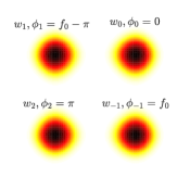
(a)	(b)

Figure 1: (color online) (a): Schematic three-dimensional states density and the trapping potential of the four-site system (in arbitrary units). (b): Localized states $w_{k}$ at the plane $z=0$, also the peculiar set of initial values of the phases are indicated.

We further investigate if the peculiar order parameter could also be another stationary solution of the GP equation gros61 ,

$$\left[-\frac{\hbar^{2}}{2m}\nabla^{2}+V_{\text{trap}}+g\,|\psi(\mathbf{r})|^{2}\right]\psi(\mathbf{r})=\mu\,\psi(\mathbf{r}),$$ (7)

where $\mu$ is the chemical potential and $g=4\pi\hbar^{2}a/m$ is the interaction strength among atoms with $a$ being their $s$-wave scattering length.

The normalized-to-unity order parameter associated to the peculiar points reads,

$$\psi_{M}({\mathbf{r}},t)=\frac{1}{2}[w_{0}(\mathbf{r})-w_{2}(\mathbf{r})]-\frac{1}{2}[{w}_{1}(\mathbf{r})-{w}_{-1}(\mathbf{r})]e^{if_{0}}$$ (8)

which in terms of GP stationary states can be written as

$$\psi_{M}({\mathbf{r}})=\frac{1}{2}\left[(1+ie^{if_{0}})\psi_{1}({\mathbf{r}})+(1-ie^{if_{0}})\psi_{-1}({\mathbf{r}})\right]\,.$$ (9)

The peculiar states are therefore a superposition of vortex states with opposite circulation. Since the states $\psi_{1}({\mathbf{r}})$ and $\psi_{-1}({\mathbf{r}})$ have the same chemical potential $\mu_{1}=\mu_{-1}$ and verify $\psi_{1}({\mathbf{r}})=\psi^{*}_{-1}({\mathbf{r}})$, applying the GP equation (7) to $\psi_{M}$ we obtain,

$$\left[-\frac{\hbar^{2}}{2m}\nabla^{2}+V_{\text{trap}}+g\,|\psi_{M}(\mathbf{r})|^{2}\right]\psi_{M}({\mathbf{r}})=\mu_{1}\,\psi_{M}({\mathbf{r}})\\ -gN\cos(f_{0})\imaginary\left(\psi_{1}^{2}({\mathbf{r}})\right)\left[\real(\psi_{1})-\imaginary(\psi_{1})e^{if_{0}}\right]$$ (10)

where in addition, we have that

$$\imaginary\left(\psi_{1}^{2}({\mathbf{r}})\right)=\frac{1}{4}[w_{0}({\mathbf{r}})-w_{2}({\mathbf{r}})]\,[w_{1}({\mathbf{r}})-w_{-1}({\mathbf{r}})]$$ (11)

is almost vanishing if the WL functions are well localized as it is in the present case. Therefore, these peculiar stationary points can be regarded as quasi-stationary solutions of the GP equation.

For the particular case of $f_{0}=\pm\pi/2$, the second term of the right hand side of Eq. (10) vanishes and thus the order parameter is an exact solution of the GP equation. Otherwise, a general value of $f_{0}$ generates an entire continuous family of states that shows a collective motion independent of time. The $\psi_{\pm 1}$ stationary solutions can be regarded as particular cases of Eq. (9) with maximum angular momentum. On the other hand, for $f_{0}=0$ we have $\psi_{M}({\mathbf{r}})=\frac{1}{2}\left[(1+i)\psi_{1}({\mathbf{r}})+(1-i)\psi_{-1}({\mathbf{r}})\right]$ which is real, hence its angular momentum is zero. Nevertheless an active vortex dynamics is present, due to the nonzero circulation of $\psi_{\pm 1}$. The same holds for $f_{0}=\pi$.

We want to remark that such a family of stationary solutions of the M model does not necessarily exist in ring lattices with an arbitrary number of wells as it can be straightforwardly deduced from the dynamical equations (2) and (LABEL:ncmode2hn). For example, for $N_{c}=3$ even though the degenerate stationary states with winding numbers $n=\pm 1$ are also present, the corresponding stationary points in the phase diagram only exist as isolated points.

IV.2 Nonstationary BON states

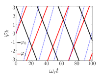
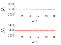
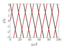
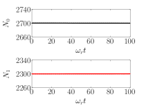
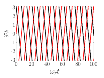
Figure 2: Populations (left column) and phase differences (right column) as function of time, from top to bottom for $\Delta N=100$, $200$, and $400$ with $f_{0}(0)=-\pi$. The solid lines correspond to GP simulations and the dashed lines to the M model. Black and red lines correspond to $N_{k}$ and $\varphi_{k}$ with $k=0$ and $k=1$, respectively. The dotted blue lines in the top right panel illustrates the prediction of the M model with the bare $U$.

When the numbers of particles of alternate sites are equal and the phases maintain their peculiar relation: $\phi_{0}=0$, $\phi_{1}=f_{0}-\pi$, $\phi_{2}=\pi$, and $\phi_{-1}=f_{0}$, the site populations do not evolve. This condition gives rise to very special dynamical states where $f_{0}$ becomes time dependent. This is shown in Fig. 2 where we compare the evolution of the occupation numbers and phase differences using full three-dimensional GP simulations with the dynamics arising from the M model. The selected initial population differences, from top to bottom, are $\Delta N=100$, $200$, and $400$, where $\Delta N=N_{0}-N_{1}$ and $f_{0}(0)=-\pi$. From Fig. 2 it may be seen that in all cases the number of particles in each site remains fixed in time, whereas their phase differences evolve faster for larger imbalances. We have further investigated the GPE dynamics for imbalances up to $\Delta N=3\times 10^{3}$ and verified that the populations remain constant within $0.1\%$ accuracy.

These family of states bear some resemblance to self-trapped states; however, there are many important differences compared to the well-known ST dynamics in double well potentials. First of all, the population imbalance can be arbitrarily small. Instead, to reach these states, it is only necessary to achieve the peculiar phases described above, being $f_{0}(0)$ an arbitrary value (given that $n_{k}=n_{k+2}$). Second, the hopping parameters $J$ and $F$ play no role in the dynamics, hence we cannot associate the emergence of the BON states to the small enough tunneling energy splitting like in the ST regime in two wells albiez05 .

The BON state normalized to unity reads,

$$\psi_{M}({\mathbf{r}},t)=\sqrt{n_{0}}[{w}_{0}(\mathbf{r})-{w}_{2}(\mathbf{r})]-\sqrt{n_{1}}[{w}_{1}(\mathbf{r})-{w}_{-1}(\mathbf{r})]e^{if_{0}(t)}$$ (12)

which written in terms of GP stationary states yields,

$$\psi_{M}({\mathbf{r}})=\left(\sqrt{n_{0}}+i\sqrt{n_{1}}e^{if_{0}(t)}\right)\psi_{1}({\mathbf{r}})\\ +\left(\sqrt{n_{0}}-i\sqrt{n_{1}}e^{if_{0}(t)}\right)\psi_{-1}({\mathbf{r}})\,.$$ (13)

In order to obtain $f_{0}(t)$ one can rewrite Eqs. (LABEL:ncmode2hn) and extract the evolution of $f_{0}(t)$ from $\hbar\,\dot{\varphi_{k}}=(n_{k-1}-n_{k})NU_{\text{eff}}$. This yields

$$f_{0}(t)=\frac{1}{\hbar}U_{\text{eff}}\Delta N\,t+f_{0}(0),$$ (14)

which in turns completely defines all the phase differences at any time within the M model. In particular, we have $\varphi_{0}(t)=-f_{0}(t)$ and $\varphi_{1}(t)=f_{0}(t)-\pi$. We note that for $n_{0}=n_{1}$ the state (13) coincides with the peculiar state (9).

It is important to point out here, that the perfect agreement between the results of GP equation and the M model observed in Fig. 2 is due to the proper definition of the onsite interaction energy parameter $U_{\mathrm{eff}}=2.27\times 10^{-3}\hbar\omega_{r}$ jezek13a , jezek13b , instead of using the bare value $U=3.16\times 10^{-3}\hbar\omega_{r}$. To illustrate such a difference, we included in Fig. 2 the evolution of $\varphi_{1}(t)$ for $\Delta N=100$ using the bare parameter $U$. Hence, we confirm the accuracy on the calculation of the effective onsite interaction energy parameter also in this dynamical regime.

To conclude we note that using Eq. (14) one can obtain the time period for the phase differences,

$$T_{M}=\frac{2\pi\hbar}{U_{\text{eff}}\Delta N}.$$ (15)

which turns to be also the time period of the persistent and collective oscillation around the ring.

IV.2.1 Angular momentum

An additional evidence of this dynamical regime is reflected in the time evolution of other observables. In particular, we shall show that within the M model the angular momentum exhibits a sinusoidal behavior as a function of time with a period $T_{M}$.

The expectation value per particle of a general observable $\widehat{O}$, considering an arbitrary state in the M model is given by

$$\langle\widehat{O}\rangle = \sum_{k}n_{k}\langle w_{k}|\widehat{O}|w_{k}\rangle$$

$$+ 2\sum_{k}\sqrt{n_{k}n_{k+1}}\real\left[e^{i(\phi_{k}-\phi_{k+1})}\langle w_{k+1}|\widehat{O}|w_{k}\rangle\right].$$

Since each well is equivalent to all others unless a discrete rotation, we have $\langle w_{k}|\widehat{O}|w_{k}\rangle=\langle w_{0}|\widehat{O}|w_{0}\rangle$ and $\langle w_{k+1}|\widehat{O}|w_{k}\rangle=\langle w_{1}|\widehat{O}|w_{0}\rangle$ for all $k$. Hence, the expectation value becomes

$$\langle\widehat{O}\rangle = \langle w_{0}|\widehat{O}|w_{0}\rangle$$ (17)

$$+ 2\sum_{k}\sqrt{n_{k}n_{k+1}}\real\left[e^{-i\varphi_{k+1}}\langle w_{1}|\widehat{O}|w_{0}\rangle\right].\,$$

For the $z$-component of the angular momentum we have $\widehat{O}=\widehat{L}_{z}=-i\hbar\frac{\partial}{\partial\theta}$ and then taking into account that the localized states can be chosen as real functions, one obtains the expectation value of angular momentum

$$\langle\widehat{L}_{z}\rangle=-2\hbar\langle w_{1}|\frac{\partial}{\partial\theta}|w_{0}\rangle\sum_{k}\sqrt{n_{k}n_{k+1}}\sin{\varphi_{k+1}}\,.$$ (18)

In a BON state with initial condition $f_{0}(0)=-\pi$, as $\sin{\varphi_{k}}=-\sin{f_{0}(t)}$ for every $k$, we can write

$$\langle\widehat{L}_{z}\rangle=-8\hbar\sqrt{n_{0}n_{1}}\langle w_{1}|\frac{\partial}{\partial\theta}|w_{0}\rangle\sin\left({\frac{1}{\hbar}U_{\text{eff}}\Delta Nt}\right)$$ (19)

where the bracket involving the localized states is a negative number. As expected, the period of this sinusoidal function is $T_{M}$. Furthermore, one can see that the stationary state Eq. (8), corresponding to $\Delta N=0$, yields a constant angular momentum proportional to $\sin(f_{0})$.

IV.2.2 Underlying dynamics

Although the population in each well remains completely fixed, the order parameter evolves in time and exhibit spatial oscillations. In order to analyze such a dynamics we first investigate the evolution of the density profile. Using the BON state expression given by Eq. (12), the evolution of the density $\rho_{M}({\mathbf{r}},t)=|\psi_{M}({\mathbf{r}},t)|^{2}$ within the M model is given by

$$\frac{\partial\rho_{M}({\mathbf{r}},t)}{\partial t}=2\sqrt{n_{0}n_{1}}\dot{f_{0}}(t)\,\sin f_{0}(t)\,\\ \times[{w}_{0}(\mathbf{r})-{w}_{2}(\mathbf{r})][{w}_{1}(\mathbf{r})-{w}_{-1}(\mathbf{r})],$$ (20)

with $\hbar\dot{f_{0}}(t)=U_{\text{eff}}\Delta N$ (cf. Eq. (14)). Equation (20) implies that $\rho_{M}({\mathbf{r}},t)$ is approximately stationary within each well, where the overlap between the WL functions of neighboring sites is negligible. Whereas the density variations are confined to the inter-well regions or junctions where the localized states do overlap. Moreover, one can infer the change of sign of $\partial\rho_{M}({\mathbf{r}},t)/\partial t$ at the junctions by analyzing Eq. (20). One can thus conclude that particles oscillate across both junctions of a given site without changing its net population. Furthermore, the maximum and minimum density variations during the evolution occur at times $t_{M}$ and $t_{m}$ when $f_{0}(t_{M})=0$ and $f_{0}(t_{m})=\pi$, respectively.

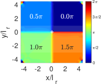
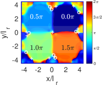
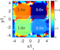
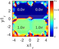
Figure 3: Phase snapshots at the $z=0$ plane obtained from the M model (left column) and from GP simulations (right column) for $\Delta N=200$. The coordinates $x$ and $y$ are divided by $l_{r}=\sqrt{\hbar/(m\omega_{r})}$. The GP times, from top to bottom of the right (panel/column), correspond to : $t_{a}=3.4\omega_{r}^{-1}$, $t_{b}=6.9\omega_{r}^{-1}$, $t_{c}=10.3\omega_{r}^{-1}$, and $t_{d}=13.7\omega_{r}^{-1}$. The plus signs (empty circles) indicate the vortex (antivortex) locations. The indicated phase values correspond to the local phases evaluated at each site center.

The sense of the particles flow across the junctions can be read off from the spatial profiles of the phases $\phi(\mathbf{r},t)$ of the wavefunction. In Fig. 3 we show snapshots of these phases at several times in the $z=0$ plane obtained from both $\psi_{M}({\mathbf{r}},t)$ and $\psi_{\text{GP}}({\mathbf{r}},t)$ in the left and right panels, respectively. In both cases we have subtracted a global phase $\phi_{0}(t)$ from $\phi(\mathbf{r},t)$ in order to better observe the dynamics. The initial condition is $\Delta N=200$ and $f_{0}=-\pi$, which yield a multimode period $T_{M}\simeq 13.8\omega_{r}^{-1}$, in sharp contrast to $2\pi\hbar/(U\Delta N)=9.95\omega_{r}^{-1}$ that would be obtained with the bare onsite interaction.

In the left column, from top to bottom, we show the phase $\phi_{M}({\mathbf{r}},t)$ obtained from the order parameter $\psi_{M}({\mathbf{r}},t)$ for the aforementioned configurations at several times: a) at $t=T_{M}/4$ ($f_{0}=-\pi/2$), there is a $\pi/2$ difference between neighboring sites and the velocity field corresponds to that of a vortex with a phase gradient in the counterclockwise direction, b) at $t=T_{M}/2$ ($f_{0}=0$), the phase difference between the right and left sites is $\pi$, which corresponds to a vanishing velocity field, c) at $t=3T_{M}/4$ ($f_{0}=\pi/2$), there is a $-\pi/2$ difference between neighboring sites, being the circulation clockwise as for an antivortex. Finally, d) at $t=T_{M}$ ($f_{0}=\pi$), there is a $\pi$ phase difference between the top and bottom sites. In the figure we have marked with a plus symbol and with an empty circle the presence of a vortex and an antivortex, respectively. For the M model, it can be seen that, in the left column of Fig. 3, there exists a vortex and an antivortex at the origin for the configurations: a) $t=T_{M}/4$ and c) $t=3/4T_{M}$, in agreement with distributions described above. In the model, the vortex (antivortex) remains fixed at $x=0,y=0$ during the interval $0<t<T_{M}/2$ ($T_{M}/2<t<T_{M}$).

On the other hand, on the right column of Fig. 3 we show phase snapshots obtained from full 3D GP simulations for times near the four different situations previously discussed. We have observed that the GP evolutions incorporate additional fluctuations and hence the velocity circulation does not change exactly at quarters of the period $T_{M}$. Moreover, the velocity field never vanishes, as the change of its circulation is associated with a passage of vortices instead of with the appearance of a nodal surface abad11 . Nevertheless, as shown together in Fig. 3, the order parameter from the M model is able to capture rather accurately the spatial distribution of phases present in the exact GP dynamics.

In particular, from top to bottom in Fig. 3, we show the results for the GP times: $t_{a}=3.4$$\omega_{r}^{-1}$, $t_{b}=6.9$$\omega_{r}^{-1}$, $t_{c}=10.3$$\omega_{r}^{-1}$, and $t_{d}=13.7$$\omega_{r}^{-1}$. In each site we indicate the value of the local phase $\phi_{\text{GP}}({\mathbf{r}},t)$ evaluated at the center of the corresponding well to be compared with that obtained in the M model. It may be confirmed that at every time the phase difference between alternated sites is always $\pi$ as predicted by the model.

It becomes clear from the change of sign in the phase differences that the velocity field is inverted near each half period, when the extreme variations in the density at the junctions are achieved. Except for some fluctuations around such a transition, in the intermediate times the total topological charge is conserved, whereas the number and the position of the vortices may change. In particular, in the third row of the right column of Fig. 3, one vortex and two antivortices are observed with a total negative charge of $-1$ instead of the single fixed antivortex predicted by the M model.

It is worthwhile to recall that the velocity circulation is quantized along any closed curved inside the superfluid and, as established in the celebrated Helmholtz-Kelvin theorem landau95 , it is conserved during the evolution if the superfluid condition is not broken bogdan03 . As a consequence, the value of the circulation can only change when a vortex passes through the curve (phase slip) or when the density goes to zero.

Although both the GP equation and the M model must obey the Helmholtz-Kelvin theorem, the order parameter given by the multimode model cannot predict the motion of vortices or the generation of vortex-antivortex pairs, hence the change of the velocity field circulation could be only provided through the appearance of nodal surfaces. The nodal surfaces arise when the minimum in the local density is achieved, i.e., at $f_{0}=0,\pi$. For example, at $f_{0}=0$ the order parameter in Eq. (12) reduces to

$$\psi_{M}({\mathbf{r}})=\sqrt{n_{0}}[w_{0}({\mathbf{r}})-w_{2}({\mathbf{r}})]-\sqrt{n_{1}}[w_{1}({\mathbf{r}})-w_{-1}({\mathbf{r}})],$$ (21)

which corresponds to the configuration b) on the left column of Fig. 3. If all the populations were equal this condition would lead to the $x=0$ plane. In our case, the deviation from a plane is due to the difference in the populations. The intersection of the nodal surface with the plane $z=0$ can be viewed in the graph by the sharp $\pi$ change of the phase where the density goes to zero. Similarly, one can obtain the nodal surfaces for $f_{0}=\pi$, which corresponds to the configuration d). In this case the curve where the density goes to zero is around $y=0$.

In contrast with the M model, the change of the velocity circulation in the GP frame is produced by the dynamics of vortices passing through the potential barriers and may include generation of vortex-antivortex pairs. In fact, we have observed that several vortex-antivortex pairs may be spontaneously generated along the barriers, thus simulating a density closer to that of the M model nodal surface. This active dynamics of vortices around the transitions is produced in a timescale much smaller than $T_{M}$ and hence it is not possible to access the details of the vortex motion within the present numerical precision. As an illustration, we note that the last time of the depicted GP snapshots is slightly smaller than the $T_{M}$ period and there still exists an antivortex around the center of the system.

IV.2.3 Velocity field circulation

Taking into account the previous findings for the multimode model one can conclude that in one $T_{M}$ period the system passes through a sequence of phases that yields an alternating velocity field circulation between values $1$ and $-1$ along a curve that connects the four wells. The transition between these two values occurs at $f_{0}=0$ and $f_{0}=\pi$ when the order parameter develops a nodal surface. In Fig. 4 we show the velocity field circulation $\mathcal{C}=\oint\mathbf{v}\cdot d\mathbf{r}$, as a function of time using the M model and GP simulations. It may be seen that the same behavior is observed with both approaches. The M model is thus able to reproduce the behavior of the circulation although the details of the internal vortex dynamics is lost. In the GP dynamics the change of circulation is caused by the motion of vortices together with the creation or annihilation of vortex-antivortex pairs. Signatures of such a vortex dynamics could be observed in Fig. 3 where we have shown the phases around the transition. Another evidence of a vortex dynamics can also be visualized in the middle panel of Fig. 4, where an additional change of sign is produced near the transition.

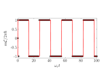
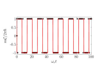
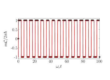
Figure 4: (color online) Velocity field circulation $\mathcal{C}$ (in units of $2\pi\hbar/m$) as a function of time for $\Delta N=100,200$, and $400$ (from top to bottom). The circles correspond to the GP results while the solid line to the results from the M model. The circulation was calculated along a square that connects the centers of the four sites in the $z=0$ plane.

IV.2.4 Stability analysis

In this section we investigate the stability of the BON states by means of a Floquet analysis Floquet , mauro4p of the multimode dynamical equations. This analysis is based on the characterization of the linear dynamics around its periodic orbits. In our case, the BON states are periodic solutions with constant populations $n_{i}(t)=n_{i}$ and linear phase differences $\varphi_{i}(t)=\varphi_{i}^{0}+(-1)^{i+1}2\pi\,{t}/{T_{M}}$ where $\varphi_{i}^{0}$ fulfill the relation: $\varphi_{0}^{0}=-f_{0}(0),\varphi_{1}^{0}=f_{0}(0)-\pi,\varphi_{2}^{0}=2\pi-f_{0}(0),\varphi_{-1}^{0}=f_{0}(0)-\pi$. The linearization of the dynamics around these states yield the non-autonomous system

$$\frac{d\bm{\delta}}{dt}=\mathbb{A}\left[n_{i}(t),\varphi_{i}(t)\right]\Bigr{|}_{\text{BON}}\cdot\bm{\delta}(t)$$ (22)

where $\bm{\delta}$ is a vector comprising both density and phase-difference fluctuations. As the BON states correspond to symmetric initial populations with peculiar phases, it is natural to consider as variables $\bm{\delta}$ the departures from a symmetric case, namely, we define

$$\delta_{1} =(n_{0}-n_{2})/2, \delta_{2}=(n_{1}-n_{-1})/2,$$ (23)

$$\delta_{3} =(\varphi_{0}-\varphi_{2})/2+\pi, \delta_{4}=(\varphi_{1}-\varphi_{-1})/2.$$ (24)

Given that the matrix $\mathbb{A}$ has a period $T_{M}$, the linearized dynamics can be characterized by the so-called Monodromy matrix $\mathbb{M}$ which contains the change of $\bm{\delta}$ after one period, i.e., $\mathbb{M}\cdot\bm{\delta}(0)=\bm{\delta}(T_{M})$. The matrix is built from the solutions of Eq. (22) with canonical initial conditions evaluated at $T_{M}$ Floquet , mauro4p . In Fig. 5 we depict elements of $\mathbb{M}$ showing the effect of an initial population fluctuation. The orbits are regular if the perturbed system remains near the initial one after a period. This happens when $\mathbb{M}_{ii}\simeq 1$ and $\mathbb{M}_{i\neq j}\simeq 0$. On the contrary, when the fluctuations are enhanced ($|\mathbb{M}_{ij}|\gg 1$), the orbits are unstable. This may be observed in Fig. 5 for low imbalances.

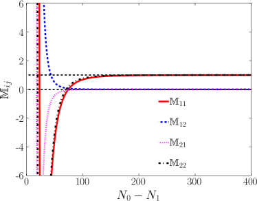
Figure 5: Selected elements of the Monodromy matrix $\mathbb{M}_{ij}$ as functions of the particle imbalance $N_{1}-N_{2}$ of BON states with $f_{0}(0)=\pi$. The horizontal dashed lines mark the values $\mathbb{M}_{ij}=0,1$.

For the peculiar stationary states ($\Delta N=0$), the linear system is time-independent and the problem reduces to a straightforward diagonalization of $\mathbb{A}$ to obtain the excitation frequencies $\tilde{\omega}$ corresponding to the Bogoliubov collectives modes in the case of the full GPE. The four frequencies are found to be

$$\tilde{\omega}=\pm\sqrt{F^{2}\,\cos^{2}f_{0}\pm K\frac{NU_{\text{eff}}}{2}\cos f_{0}-(K+F)^{2}}$$ (25)

where $K=2J+F$. As $NU_{\text{eff}}\gg K,F$, the most stable frequency for a given system is attained for peculiar states with $f_{0}=\pm\pi/2$ which in turn yield an imaginary frequency $\tilde{\omega}^{2}=-(K+F)^{2}$. Therefore all $f_{0}$ give rise to dynamically unstable peculiar states. The stability of stationary vortex states ($f_{0}=\pm\pi/2$) has been previously investigated in Paraoanu2003 for circular arrays of BECs, finding that only states with circulation below $N_{c}/4$ are stable.

IV.2.5 Proposed experimental test

The correct preparation of BON states requires a special sequence of phases and symmetric initial populations ($n_{k}=n_{k+1}$). While the common approach to experimentally measure both of them is by means of TOF and absorption images, the simple dynamics of BON states offers an alternative way to confirm its correct realization using TOF images only. Given that the relative phases among neighboring sites are revealed in the interference patterns during the TOF expansion albiez05 , it could be verified that they obey the peculiar sequence of phases at all times. According to Eq. (14), in this case $f_{0}(t)$ must be a linear function whose slope $\gamma$ relates to the particle imbalance as

$$\Delta N=\frac{\hbar\gamma}{U_{\mathrm{eff}}},$$ (26)

which might probe to be a more accurate measure than the direct estimate from absorption images. On the other hand, since Eq. (26) requires the use of $U_{\mathrm{eff}}$ instead of the bare $U$, it may also serve to confirm its numerical value. By using $U$ the relative error on the imbalances could be as large as of order 20-30%, depending on the number of particles mauro17 .

Due to the experimental uncertainty, absorption images may not be able to reveal a slightly broken symmetry of the population configuration. However, the evolution of the phases will depart from linearity and will not be determined by the single function $f_{0}$.

V Extension to larger number of wells

It is possible to extend the peculiar and BON states to larger number of wells provided the sequence of phases $...0,f_{0}-\pi,\pi,f_{0},0...$ is repeated $l=N_{c}/4$ times around the ring lattice, and the populations alternate between two values, with $n_{2k}=n_{0}$ and $n_{2k+1}=n_{1}$. This is only possible when the number of wells are multiples of 4. Taking into account these conditions in Eq. (1) and using Eq. (4) to eliminate the WL functions $w_{k}$, we can write the following BON order parameter in terms of GP stationary states,

$$\psi_{M}({\mathbf{r}}) = \frac{\sqrt{N_{c}}}{2}\left[(\sqrt{n_{0}}+i\sqrt{n_{1}}e^{if_{0}(t)})\psi_{\frac{N_{c}}{4}}({\mathbf{r}})\right.$$ (27)

$$+ \left.(\sqrt{n_{0}}-i\sqrt{n_{1}}e^{if_{0}(t)})\psi_{-\frac{N_{c}}{4}}({\mathbf{r}})\right]\,.$$

It is straightforward to show that $f_{0}(t)$ still obeys Eq. (14), and thus the corresponding time period is also given by Eq. (15). Therefore, the analysis performed in the previous section can be repeated using the same procedure, including the Floquet theory. However, for these configurations the velocity field circulation alternates between $\pm N_{c}/4$ and the number of nodal surfaces at each half period is equal to $l$. Equation (27) shows that an arbitrary linear combination of $\psi_{\pm\frac{N_{c}}{4}}$ leads to the BON dynamics. For example, even though for $N_{c}=8$ it is not possible to generate the BON dynamics with a linear combination of the degenerate $\psi_{\pm 1}$ states; any linear combination of $\psi_{\pm 2}$ will indeed give rise to a BON dynamics.

Using Eq. (18) the mean value of the $z$-component of the angular momentum is given by,

$$\langle L_{z}\rangle(t)=2N_{c}\hbar\langle w_{1}|\frac{\partial}{\partial\theta}|w_{0}\rangle\sqrt{n_{0}n_{1}}\sin(f_{0}(t)).$$ (28)

If we let $n_{0}=n_{1}$ then we obtain the most general quasi-stationary states described in section IV.A:

$$\psi_{M}({\mathbf{r}}) = \frac{1}{2}\left[(1+ie^{if_{0}})\psi_{\frac{N_{c}}{4}}({\mathbf{r}})\right.$$ (29)

$$+ \left.(1-ie^{if_{0}})\psi_{-\frac{N_{c}}{4}}({\mathbf{r}})\right]\,.$$

that satisfies

$$\left[-\frac{\hbar^{2}}{2m}\nabla^{2}+V_{\text{trap}}+g\,|\psi_{M}(\mathbf{r})|^{2}\right]\psi_{M}({\mathbf{r}})=\mu_{\frac{N_{c}}{4}}\,\psi_{M}({\mathbf{r}})\\ -gN\cos(f_{0})\imaginary\left(\psi_{\frac{N_{c}}{4}}^{2}({\mathbf{r}})\right)\left[\real(\psi_{\frac{N_{c}}{4}})-\imaginary(\psi_{\frac{N_{c}}{4}})e^{if_{0}}\right]$$ (30)

Since

$$\imaginary\left(\psi_{\frac{N_{c}}{4}}^{2}\right) = \frac{1}{N_{c}}\sum_{k,k^{\prime}}w_{k}w_{k^{\prime}}\sin\left[\frac{\pi}{2}(k+k^{\prime})\right]$$

the states Eq. (29) can be regarded as quasi-stationary solutions of the GP equation when the $w_{k}$ are well localized functions.

VI Summary and concluding remarks

We have studied a particular dynamical regime of a Bose-Einstein condensate in a ring-shaped lattice which possesses a set of states with fixed number of particles in each site and a simple dynamics in their phases. The same distribution of phases along the sites that gives rise to such nonstationary states has been shown to generate a continuous family of stationary points in the phase space of the multimode model. Such peculiar states have constant nonzero angular momentum, when all the populations are equal, and include two states that correspond to exact GP stationary solutions.

We have shown that the nonlinearity of the GP equation governs the dynamics within this regime and that it is responsible for the population blocking in the nonstationary states. In contrast to the self-trapping phenomenon this effect does not possess a lower bound for the population imbalance.

We have studied the time evolution of BON states using both the multimode model and the three-dimensional GP equation finding an excellent agreement in the populations in each site and in their phase differences. This accuracy was possible due to the inclusion of the effective interaction energy parameter instead of the bare one. Even though the multimode model was unable to account for the motion of individual vortices and the creation/annihilation of vortex-antivortex pairs, it was demonstrated that it correctly predicts the evolution of the velocity circulation and angular momentum, characterizing this regime as a persistent current oscillating around the lattice.

By performing a Floquet stability analysis of the blocked populations states, we have verified that their dynamics is regular for the particle imbalances here considered. In a four-well system these states could, in principle, be experimentally achieved by initially manipulating the position of the potential barriers in order to have different populations or by using an elliptic trap in the $(x,y)$ plane with their axis forming a $\pi/4$ angle during a short time and then reverting the potential to a circular harmonic trap. A simple way to produce the initial distribution of phases would be to start with the same state as we have used in our numerical calculations. This could be achieved by illuminating half of the condensate (e.g., $x>0$ ) with an additional laser for a period of time until it develops a $\pi$ phase difference between the half spaces $x>0$ and $x<0$. However, any other initial distribution of phases seems feasible using a Spatial Light Modulator (SLM) slm1 , slm2 , slm3 , and hence also the whole family of stationary M-model states could be directly generated. Furthermore, given that all the phases loose their dependence on a single linear function as soon as the symmetric condition on the site populations is lifted, these states could be first tested to adjust the population in alternate wells with arbitrary imbalances. A second phase imprinting application could then be used to generate the desired state. Since the BON states present a simple analytical form for the phase difference between neighboring sites, it could also allow to measure the initial population imbalance by means on interference patterns in TOF images, rather than absorption images.

*

Appendix A Parameters

The multimode model parameters are defined by

$$J=-\int d^{3}{\bf r}\,\,w_{0}({\bf r})\left[-\frac{\hbar^{2}}{2m}{\bf\nabla}^{2}+V_{\text{trap}}({\bf r})\right]w_{1}({\bf r}),$$ (32)

$$U=g\int d^{3}{\bf r}\,\,w_{0}^{4}({\bf r}),\quad\text{and}$$ (33)

$$F=-N\,g\int d^{3}{\bf r}\,\,w_{0}^{3}({\bf r})w_{1}({\bf r}).$$ (34)

Together with the calculation of these parameters by the preceding definitions we have followed the alternative method outlined in Ref. jezek13b which involves directly the energies of the GP stationary states. Both approaches have proven to yield values equal in less than one percent. We note that we have disregarded the parameter that involves products of neighboring densities because, for the present system, its contribution turned out to be negligible.

This work was supported by CONICET and Universidad de Buenos Aires through grants PIP 11220150100442CO and UBACyT 20020150100157BA, respectively.

References

- [1] A. Smerzi, S. Fantoni, S. Giovanazzi, and S. R. Shenoy, Phys. Rev. Lett. 79, 4950 (1997).
- [2] S. Raghavan, A. Smerzi, S. Fantoni, and S. R. Shenoy, Phys. Rev. A 59, 620 (1999).
- [3] D. Ananikian and T. Bergeman, Phys. Rev. A 73, 013604 (2006).
- [4] X. Y. Jia, WeiDong Li, and J. Q. Liang, Phys. Rev. A 78, 023613 (2008).
- [5] M. Melé-Messeguer, B. Juliá-Díaz, M. Guilleumas, A. Polls and A. Sanpera, New J. Phys. 13, 033012 (2011).
- [6] M. Abad, M. Guilleumas, R. Mayol, M. Pi, and D. M. Jezek, Europhys. Lett. 94, 10004 (2011).
- [7] M. Nigro, P. Capuzzi, H. M. Cataldo, and D. M. Jezek, Eur. Phys. J. D 71, 297 (2017).
- [8] T. Mayteevarunyoo, B. A. Malomed, and G. Dong, Phys. Rev. A 78, 053601 (2008); B. Xiong, J. Gong, H. Pu, W. Bao, and B. Li, Phys. Rev. A 79, 013626 (2009); Qi Zhou, J. V. Porto, and S. Das Sarma, Phys. Rev. A 84, 031607 (2011); B. Cui, L.C. Wang, and X. X. Yi, Phys. Rev. A 82, 062105 (2010); M. Abad, M. Guilleumas, R. Mayol, M. Pi, and D. M. Jezek, Phys. Rev. A 84, 035601 (2011).
- [9] M. Albiez, R. Gati, J. Fölling, S. Hunsmann, M. Cristiani, and M. K. Oberthaler, Phys. Rev. Lett. 95, 010402 (2005).
- [10] Michael Albiez, Observation of Nonlinear Tunneling of a Bose-Einstein Condensate in a Single Josephson Junction (PhD thesis), University of Heidelberg, 2005
- [11] Rudolf Gati, Bose-Einstein Condensates in a Single Double Well Potential (PhD thesis), University of Heidelberg, 2007.
- [12] Th. Anker, M. Albiez, R. Gati, S. Hunsmann, B. Eiermann, A. Trombettoni, and M. K. Oberthaler, Phys. Rev. Lett. 94, 020403 (2005).
- [13] Bingbing Wang, Panming Fu, Jie Liu, and Biao Wu, Phys. Rev. A 74, 063610 (2006).
- [14] C. E. Creffield, Phys. Rev. A 75, 031607(R) (2007). Ju-Kui Xue, Ai-Xia Zhang, and Jie Liu, Phys. Rev. A 77, 013602 (2008). T. J. Alexander, E. A. Ostrovskaya, and Y. S. Kivshar, Phys. Rev. Lett. 96, 040401 (2006). Bin Liu, Li-Bin Fu, Shi-Ping Yang, and Jie Liu, Phys. Rev. A 75, 033601 (2007).
- [15] S. K. Adhikari, J. Phys. B: At. Mol. Opt. Phys. 44, 075301 (2011).
- [16] S. De Liberato and C. J. Foot, Phys. Rev. A 73, 035602 (2006).
- [17] Geva Arwas, Amichay Vardi, and Doron Cohen, Phys. Rev. A 89, 013601 (2014).
- [18] M. Nigro, P. Capuzzi, H. M. Cataldo, and D. M. Jezek, Phys. Rev. A 97, 013626 (2018).
- [19] D. M. Jezek, P. Capuzzi, and H. M. Cataldo, Phys. Rev. A 87, 053625 (2013).
- [20] D. M. Jezek and H. M. Cataldo, Phys. Rev. A 88, 013636 (2013).
- [21] R. Kolovsky, New J. Phys. 8, 197 (2006).
- [22] A. Gallemí, M. Guilleumas, J. Martorell, R. Mayol, A. Polls, and B. Juliá-Díaz, New J. Phys. 18, 075005 (2016).
- [23] A. Burchianti, C. Fort, and M. Modugno, Phys. Rev. A 95, 023627 (2017).
- [24] K. Henderson, C. Ryu, C. MacCormick, and M. G. Boshier, New J. Phys. 11, 043030 (2009).
- [25] H. M. Cataldo and D. M. Jezek, Phys. Rev. A 84, 013602 (2011).
- [26] E. P. Gross, Nuovo Cimento 20, 454 (1961); L. P. Pitaevskii, Zh. Eksp. Teor. Fiz. 40, 646 (1961) [Sov. Phys. JETP 13, 451 (1961)].
- [27] D. M. Jezek and H. M. Cataldo, Phys. Rev. A 83, 013629 (2011).
- [28] L. D. Landau and E. M. Lifshitz, Fluid Mechanics New York: Butterworth-Heinemann (1995).
- [29] D. Bogdan and S. Krzysztof, J. Phys. A: Math. Theor. 36, 2339 (2003).
- [30] C. Chicone, Ordinary Differential Equations with Applications, 2nd ed. (Springer, New York, 2006).
- [31] Gh.-S. Paraoanu, Phys. Rev. A 67, 023607 (2003).
- [32] S. Burger, K. Bongs, S. Dettmer, W. Ertmer, K. Sengstock, A. Sanpera, G. V. Shlyapnikov, and M. Lewenstein, Phys. Rev. Lett. 83, 5198 (1999).
- [33] J. Denschlag, J. E. Simsarian, D. L. Feder, C. W. Clark, L. A. Collins, J. Cubizolles, L. Deng, E. W. Hagley, K. Helmerson, W. P. Reinhardt, S. L. Rolston, B. I. Schneider, and W. D. Phillips, Science 287, 97 (2000), http://science.sciencemag.org/content/287/5450/97.
- [34] Avinash Kumar, Romain Dubessy, Thomas Badr, Camilla De Rossi, Mathieu de Goer de Herve, Laurent Longchambon, and Helene Perrin, arXiv:1801.04792.