From megahertz to terahertz qubits encoded in molecular ions: theoretical analysis of dipole-forbidden spectroscopic transitions in N$\mathbf{{}_{2}^{+}}$

Abstract

Recent advances in quantum technologies have enabled the precise control of single trapped molecules on the quantum level. Exploring the scope of these new technologies, we studied theoretically the implementation of qubits and clock transitions in the spin, rotational, and vibrational degrees of freedom of molecular nitrogen ions including the effects of magnetic fields. The relevant spectroscopic transitions span six orders of magnitude in frequency illustrating the versatility of the molecular spectrum for encoding quantum information. We identified two types of magnetically insensitive qubits with very low (“stretched”-state qubits) or even zero (“magic” magnetic-field qubits) linear Zeeman shifts. The corresponding spectroscopic transitions are predicted to shift by as little as a few mHz for an amplitude of magnetic-field fluctuations on the order of a few mG translating into Zeeman-limited coherence times of tens of minutes encoded in the rotations and vibrations of the molecule. We also found that the Q(0) line of the fundamental vibrational transition is magnetic-dipole allowed by interaction with the first excited electronic state of the molecule. The Q(0) transitions, which benefit from small systematic shifts for clock operation and high sensitivity to a possible variation in the proton-to-electron mass ratio, were so far not considered in single-photon spectra. Finally, we explored possibilities to coherently control the nuclear-spin configuration of N${}_{2}^{+}$ through the magnetically enhanced mixing of nuclear-spin states.

I Introduction

Over the past two decades, a range of different methods have been devised for the generation of cold trapped molecules in the gas phase. These include molecular-beam slowing and trapping van de Meerakker et al. (2012); Segev et al. (2019), direct laser cooling Anderegg et al. (2018); McCarron et al. (2018); Caldwell et al. (2019), assembly from ultracold atoms Moses et al. (2017), and sympathetic cooling Mølhave and Drewsen (2000); Tong et al. (2010). In this context, experiments in which single molecular ions are co-trapped with single atomic ions Wolf et al. (2016); Chou et al. (2017); Sinhal et al. (2020); Chou et al. (2020); Lin et al. (2020); Najafian et al. (2020) show excellent prospects for achieving the long-standing goal of gaining full control over the quantum state and dynamics of single isolated molecules. In these experiments, a quantum-logic approach Schmidt et al. (2005) is pursued in which the co-trapped atomic ion is used to detect the state of the molecular ion. Coherent Rabi and Ramsey spectroscopy Chou et al. (2017, 2020), quantum-non demolition state detection Wolf et al. (2016); Sinhal et al. (2020); Najafian et al. (2020) and atom-molecule entanglement Lin et al. (2020) have recently been demonstrated.

A full control over the quantum states of cold and trapped molecules will enable improved experiments in the realm of precision spectroscopy. Applications range from precisely validating existing physical theories such as quantum electrodynamics Semeria et al. (2020); Alighanbari et al. (2018); Biesheuvel et al. (2016), testing fundamental concepts Safronova et al. (2018); DeMille et al. (2017) such as a possible time variation of physical constants Schiller and Korobov (2005); Flambaum and Kozlov (2007) and the putative existence of new forces of nature Salumbides et al. (2013), benchmarking molecular-structure theory Chou et al. (2020); Hölsch et al. (2019), performing controlled chemical reactions Sikorsky et al. (2018); Dörfler et al. (2019), to implementing new time standards based on narrow rovibrational molecular transitions in the mid-infrared spectral domain Germann et al. (2014); J.-Ph. Karr (2014); Schiller et al. (2014).

While spectroscopy can be performed in a destructive fashion Willitsch (2011); Germann et al. (2014), the newly developed methods for non-destructive detection and coherent manipulation of molecular ions promise an increase of several orders of magnitude in the experimental duty cycle Sinhal et al. (2020); Meir et al. (2019). This increase will result in a markedly improved spectroscopic sensitivity and, therefore, precision. Another exciting aspect of this technology is the implementation of molecular qubits which can be used for applications in quantum computation DeMille (2002), simulation Blackmore et al. (2018), metrology Manovitz et al. (2019), and communication Kimble (2008).

Here, we studied theoretically the implementation of molecular qubits and their prospective application for spectroscopic precision measurements in the homonuclear ¹⁴N${}_{2}^{+}$ molecular ion. We chose this molecule due to its prospects for investigating a possible time variation of the electron-to-proton mass ratio Kajita et al. (2014) and for serving as a mid-infrared (MIR) frequency standard Kajita (2015); J.-Ph. Karr (2014); Schiller et al. (2014). These applications are enabled by the lack of a permanent dipole moment of the molecule such that rovibrational transitions within the same electronic state are electric-dipole forbidden. These transitions only become allowed in higher order and thus exhibit very narrow natural linewidths Germann et al. (2014); Germann (2016) and low to vanishing susceptibility to external perturbations such as blackbody radiation and stray electric fields Kajita et al. (2014); Kajita (2015). These qualities also make N${}_{2}^{+}$ an excellent system for encoding qubits in its rovibrational state manifold in which radiative lifetimes of excited states are estimated to be on the order of months to years Germann (2016).

While electric perturbations are inherently small in N${}_{2}^{+}$ (see discussion in Ref. Kajita et al. (2014) and in Appendix A), the molecular states are strongly coupled to external magnetic fields due to the doublet electron-spin character of the molecule Kajita (2015). Finite magnetic fields are present in a typical experimental apparatus, especially in ion-trapping experiments in which they are a perquisite for operation. Moreover, an external magnetic field is used to lift the degeneracy of Zeeman states and to define the quantization axis of qubits realized in atomic systems. Therefore, there is a need for a comprehensive theoretical analysis of the influence of external magnetic fields on the rovibrational states of N${}_{2}^{+}$.

Here, we expanded the theory on the hyperfine structure of N${}_{2}^{+}$ in Ref. Mansour et al. (1991) to include the Zeeman effect. We numerically diagonalized the effective molecular Hamiltonian of N${}_{2}^{+}$ in the electronic ground-state, $X^{2}\Sigma_{g}^{+}$, including the interaction with magnetic fields. From the energy-level structure thus derived, we analyzed several classes of spectroscopic transitions from the radio (MHz) to mid-infrared (THz) domains. The different types of transitions (Zeeman, hyperfine-structure, fine-structure, rotational and vibrational) are discussed with respect to their applications as qubits and in precision spectroscopy.

Magnetic-field insensitive transitions are important since magnetic-field fluctuations are amongst the dominant effects causing decoherence of qubit superpositions. The use of magnetic-field-insensitive transitions for molecular qubits can dramatically increase their coherence time Wang et al. (2017). We identified “magic” transitions Langer et al. (2005) for which the relative Zeeman shift between the energy levels involved cancels to first order at a experimentally practicable magnetic-field strength of a few Gauss. These transitions allow for magnetic-field-limited coherence times of tens of minutes in rotational and vibrational qubits at realistic levels of magnetic field noise without the need for magnetic shielding or active magnetic-noise cancellation. We also identified transitions in which the linear Zeeman shift is only on the order of 10 Hz/G irrespective of the magnetic-field strength. The latter are transitions between ”stretched” states of different ro-vibrational manifolds in the electronic ground state for which the contribution of the electron spin to the Zeeman shift largely cancels Kajita et al. (2014); Caldwell et al. (2020). These “streched” magnetic-insensitive transitions are unique to molecular qubits.

Previous experimental and theoretical works on N${}_{2}^{+}$ analyzed the S(0) rotational component of the fundamental vibrational transition Germann et al. (2014); Kajita (2015), i.e, the transition from the vibrational and rotational ground state to first vibrationally and second rotationally excited state. This transition is single-photon allowed by electric-quadrupole (E2) selection rules. The corresponding Q(0) transition, i.e, the pure vibrational transition with no excitation of the rotation, was predicted to exhibit superior properties for clock and precision-spectroscopy applications due to smaller systematic shifts Kajita et al. (2014). Here, we show that the Q(0) transitions, which were previously considered to be forbidden in single-photon excitation in the present system Kajita (2015), are actually magnetic dipole (M1) allowed through the anisotropy of the interaction of the electron spin with the magnetic field. This is enabled by a mixing of the first excited electronic state, $A^{2}\Pi_{u}$, with the electronic ground-state, $X^{2}\Sigma_{g}^{+}$, of the nitrogen ion Bruna and Grein (2004).

In addition, we identified avoided crossings of energy levels originating from two different nuclear-spin configurations with nuclear-spin quantum numbers $I=0$ and $I=2$. The avoided crossings occur at low, experimentally accessible magnetic-field strengths of a few tens of Gauss. Around these avoided crossings, the molecular eigenstates have a mixed character of the $I=0$ and $I=2$ spin states. This magnetically enhanced nuclear-spin mixing opens up opportunities for transmuting molecular-spin states on demand by coherent two-photon processes, e.g, stimulated Raman pumping Gaubatz et al. (1990), through the highly mixed states around the avoided crossings.

Finally, we found that for some transitions, M1 coupling dominates the spectrum while for others E2 coupling prevails due to selection rules forbidding M1 coupling. We also found that hyperfine mixing terms in the Hamiltonian allow for otherwise forbidden transitions which significantly changes the spectra compared to zeroth-order expectations.

II Theory

II.1 Basis states

The molecular nitrogen ion, N${}_{2}^{+}$, in the electronic ground state, $X^{2}\Sigma_{g}^{+}$, is adequately described within the Hund’s case ($b_{\beta_{J}}$) angular momentum coupling scheme Frosch and Foley (1952) given by,

$$\mathbf{N+S=J},$$ (1)

$$\mathbf{J+I=F}.$$ (2)

Here, $\mathbf{N}$ is the rotational angular momentum in a $\Sigma$ electronic state, $\mathbf{J}$ is the angular momentum resulting from the coupling between the electron spin $\mathbf{S}$ and the rotation, and $\mathbf{F}$ is the total angular momentum including the nuclear spin $\mathbf{I}$. The Hund’s case ($b_{\beta_{J}}$) basis describing this coupling scheme is denoted by,

$$|\phi_{i}\rangle=|v,N,S,J,I,F,m\rangle.$$ (3)

Here, $v$ is the vibrational, $N$ the rotational, $S$ the electron-spin, $J$ the fine-structure (spin-rotation), $I$ the nuclear-spin and $F$ the hyper-fine quantum number. We denote the projection of the total angular momentum $\mathbf{F}$ on the axis of the external magnetic field by $m$, and $i$ is a compound index for all quantum numbers. We used an effective Hamiltonian approach Brown and Carrington (2003); Brown et al. (1978) in which global perturbations from other electronic and vibrational states are absorbed in the molecular constants. Therefore, we omit the electronic index of the basis states.

Since each ¹⁴N atom has a nuclear spin of $1$, the total nuclear spin, $I$, of the ¹⁴N${}_{2}^{+}$ molecule can take the values of $I=0,1,2$. This gives rise to different nuclear-spin-symmetry isomers with even (odd) $I$ denoted as ortho (para). In N${}_{2}^{+}$, even (odd) values of $I$ allow for only even (odd) rotational quantum numbers $N$ due to the total permutation symmetry of the molecular wavefunction imposed by the generalized Pauli principle. While our results are applicable for both spin isomers of N${}_{2}^{+}$, in this manuscript, we mainly focus on the ortho nuclear-spin isomer with $I=0,2$ which is associated with the rotational ground state of particular interest in experiments.

II.2 Effective Hamiltonian

We considered the following effective Hamiltonian for the electronic ground state, $X^{2}\Sigma_{g}^{+}$, of N${}_{2}^{+}$ Mansour et al. (1991); Balasubramanian et al. (1994); Brown and Carrington (2003),

$$\mathscrsfs{H}=\mathscrsfs{H}_{vib}+\mathscrsfs{H}_{rot}+\mathscrsfs{H}_{fs}+\mathscrsfs{H}_{hfs}+\mathscrsfs{H}_{z}.$$ (4)

The first three terms describing the vibrational, rotational and fine structure are diagonal in the Hund’s case (b) basis (Eq. 3). Their matrix elements are given by $\mathscrsfs{H}_{vib,ii}=G_{v}$, $\mathscrsfs{H}_{rot,ii}=B_{v}N(N+1)-D_{v}(N(N+1))^{2}$, and $\mathscrsfs{H}_{fs,ii}=\gamma_{v,N}(J(J+1)-N(N+1)-S(S+1))/2$. Here, the subscript $v$ indicates that the molecular constants are effective values for a given vibrational and Born-Oppenheimer electronic state, $G_{v}$ is the vibrational energy, $B_{v}$ is the rotational constant, $D_{v}$ is the centrifugal-distortion constant and $\gamma_{v,N}$ is the electron spin-rotation coupling constant which includes a centrifugal correction term $\gamma_{v,N}=\gamma_{v}+\gamma_{D_{v}}N(N+1)$ Mansour et al. (1991). The relevant spectroscopic constants are listed in Table 1. Note that our notation of the constants differs in places from the one found in the literature Mansour et al. (1991) to render it unambiguous in the present context.

Figure 1: Partial schematic of the field-free energy levels of N${}_{2}^{+}$ in the electronic ground state, $X^{2}\Sigma_{g}^{+}$ (not to scale). The states are labeled using the Hund’s case ($b_{\beta_{J}}$) basis (Eq. 3). The dashed boxes indicate the level subspaces shown in Figs. 2 and 5 where the relevant Zeeman manifolds are displayed. The color coding of the levels is identical with the one used in those figures.

The effective hyperfine-interaction Hamiltonian takes the form Mansour et al. (1991),

$$\mathscrsfs{H}_{hfs}=\mathscrsfs{H}_{b_{F}}+\mathscrsfs{H}_{t}+\mathscrsfs{H}_{eqQ}+\mathscrsfs{H}_{c_{I}}.$$ (5)

Here, $\mathscrsfs{H}_{b_{F}}$ represents the Fermi-contact interaction which has off-diagonal matrix elements in the $J$ quantum number, $\mathscrsfs{H}_{t}$ is the dipolar hyperfine interaction with off-diagonal matrix elements in $N$ and $J$, $\mathscrsfs{H}_{eqQ}$ is the electric-quadrupole hyperfine interaction with off-diagonal matrix elements in $N$, $J$ and $I$ and $\mathscrsfs{H}_{c_{I}}$ is the magnetic nuclear spin-rotation interaction which mixes states with different $J$ quantum numbers. All matrix elements are given in Appendix B, and the effective coupling constants are given in Table 1. A schematic of the resulting energy levels is shown in Fig. 1.

In the $X^{2}\Sigma_{g}^{+}$ ground state of N${}_{2}^{+}$, the effective Zeeman Hamiltonian, $\mathscrsfs{H}_{z}$, neglecting relativistic and radiative corrections Karr et al. (2008), has four first-order contributions corresponding to the interaction of the magnetic field $\mathbf{B}$ with the magnetic moments of the electron spin, rotation and nuclear spin Brown et al. (1978); Brown and Carrington (2003); Ma et al. (2009); Chen et al. (2006),

$$\mathscrsfs{H}_{z}=g_{s}\mu_{B}T^{1}_{p=0}(\mathbf{B})T^{1}_{p=0}(\mathbf{S})$$ (6)

$$-g_{r}\mu_{B}T^{1}_{p=0}(\mathbf{B})T^{1}_{p=0}(\mathbf{N})$$

$$-g_{n}\mu_{N}T^{1}_{p=0}(\mathbf{B})T^{1}_{p=0}(\mathbf{I})$$

$$+g_{l}\mu_{B}T^{1}_{p=0}(\mathbf{B})\sum\limits_{q=\pm 1}\mathscrsfs{D}^{1}_{p=0,q}(\omega)^{*}T^{1}_{q}(\mathbf{S}).$$

Here, $g_{s}$, $g_{r}$ and $g_{n}$ are the $g$-factors for the spin, rotation and nuclear spin and $\mu_{B}$ ($\mu_{N})$ is the Bohr (nuclear) magneton. The last term in $\mathscrsfs{H}_{z}$ represents the anisotropic correction to the electron-spin Zeeman interaction and $g_{l}$ is the corresponding effective g-factor. $T^{1}_{p}$ denotes a spherical tensor operator of rank 1 in the space-fixed (subscript $p$) coordinate system, $\mathscrsfs{D}^{1}_{pq}(\omega)$ is a Wigner rotation-matrix element, and the subscript $q$ denotes spherical tensor components in the molecule-fixed coordinate system. The $p=0$ component of the space-fixed coordinate system is taken to be aligned with the direction of the magnetic field, $T^{1}_{p=0}(\mathbf{B})=B_{Z}\hat{Z}$. The rotational and anisotropic spin $g$-factors, $g_{r}$ and $g_{l}$, show a non-negligible dependence on the vibrational state (see Table 1). Diagonal terms in the interaction of the magnetic field with the electronic orbital angular momentum ($\mathbf{L}$) vanish in a $\Sigma$ state and terms of higher order in the magnetic field ($\propto\mathbf{B}^{2}$) Schiff and Snyder (1939); Brown and Carrington (2003) are neglected in our analysis.

The interaction of the magnetic field with the electron spin mixes states with different $J$ and $F$ quantum numbers. The matrix-elements are given by,

$$\langle N^{\prime},S^{\prime},J^{\prime},I^{\prime},F^{\prime},m^{\prime}|T^{1}_{p=0}(\mathbf{B})T^{1}_{p=0}(\mathbf{S})|N,S,J,I,F,m\rangle=$$ (7)

$$B_{Z}\delta_{NN^{\prime}}\delta_{SS^{\prime}}\delta_{II^{\prime}}(-1)^{F^{\prime}+F-m^{\prime}+2J^{\prime}+N+S+I}$$

$$\times\sqrt{(2F^{\prime}+1)(2F+1)(2J^{\prime}+1)(2J+1)S(S+1)(2S+1)}$$

$$\times\begin{pmatrix}F^{\prime}&1&F\\ -m^{\prime}&p&m\end{pmatrix}\begin{Bmatrix}J^{\prime}&F^{\prime}&I\\ F&J&1\end{Bmatrix}\begin{Bmatrix}S&J^{\prime}&N\\ J&S&1\end{Bmatrix}.$$

The same type of mixing occurs also for the interaction with the rotational magnetic moment,

$$\langle N^{\prime},S^{\prime},J^{\prime},I^{\prime},F^{\prime},m^{\prime}|T^{1}_{p=0}(\mathbf{B})T^{1}_{p=0}(\mathbf{N})|N,S,J,I,F,m\rangle=$$ (8)

$$B_{Z}\delta_{NN^{\prime}}\delta_{SS^{\prime}}\delta_{II^{\prime}}(-1)^{F^{\prime}+F-m^{\prime}+J^{\prime}+J+N+S+I}$$

$$\times\sqrt{(2F^{\prime}+1)(2F+1)(2J^{\prime}+1)(2J+1)N(N+1)(2N+1)}$$

$$\times\begin{pmatrix}F^{\prime}&1&F\\ -m^{\prime}&p&m\end{pmatrix}\begin{Bmatrix}J^{\prime}&F^{\prime}&I\\ F&J&1\end{Bmatrix}\begin{Bmatrix}N&J^{\prime}&S\\ J&N&1\end{Bmatrix}.$$

Interaction with the nuclear spin only mixes states with different $F$ quantum numbers,

$$\langle N^{\prime},S^{\prime},J^{\prime},I^{\prime},F^{\prime},m^{\prime}|T^{1}_{p=0}(\mathbf{B})T^{1}_{p=0}(\mathbf{I})|N,S,J,I,F,m\rangle=$$ (9)

$$B_{Z}\delta_{JJ^{\prime}}\delta_{NN^{\prime}}\delta_{SS^{\prime}}\delta_{II^{\prime}}(-1)^{2F^{\prime}-m^{\prime}+J^{\prime}+I+1}$$

$$\times\sqrt{(2F^{\prime}+1)(2F+1)I(I+1)(2I+1)}\begin{pmatrix}F^{\prime}&1&F\\ -m^{\prime}&p&m\end{pmatrix}\begin{Bmatrix}I&F^{\prime}&J\\ F&I&1\end{Bmatrix}.$$

The matrix elements of the anisotropic correction to the electron-spin interaction in the Zeeman Hamiltonian are given by,

$$\langle N^{\prime},S^{\prime},J^{\prime},I^{\prime},F^{\prime},m^{\prime}|T^{1}_{p=0}(\mathbf{B})\sum\limits_{q=\pm 1}\mathscrsfs{D}_{{p=0},q}^{1}(\omega)^{*}T^{1}_{q}(\mathbf{S})|N,S,J,I,F,m\rangle=$$ (10)

$$B_{Z}\delta_{SS^{\prime}}\delta_{II^{\prime}}(-1)^{F^{\prime}-m^{\prime}+F+J^{\prime}+I^{\prime}+1+N^{\prime}}$$

$$\times\sqrt{(2F^{\prime}+1)(2F+1)(2J^{\prime}+1)(2J+1)(2N^{\prime}+1)(2N+1)S(S+1)(2S+1)}\begin{pmatrix}F^{\prime}&1&F\\ -m^{\prime}&p&m\end{pmatrix}\begin{Bmatrix}J^{\prime}&F^{\prime}&I\\ F&J&1\end{Bmatrix}$$

$$\times 2\sum\limits_{k=0,2}(2k+1)\begin{pmatrix}1&1&k\\ -1&1&0\end{pmatrix}\begin{pmatrix}N^{\prime}&k&N\\ 0&0&0\end{pmatrix}\begin{Bmatrix}J^{\prime}&J&1\\ N^{\prime}&N&k\\ S^{\prime}&S&1\end{Bmatrix}.$$

This interaction mixes different $F$,$J$ and $N$ quantum numbers.

The complete Hamiltonian given in Eq. 4 was diagonalized numerically by solving $\mathscrsfs{H}(B_{Z})\left|\psi_{k}\right\rangle=E_{k}(B_{Z})\left|\psi_{k}\right\rangle$ in the Hund’s case ($b_{\beta_{J}}$) basis (Eq. 3) to obtain the energies, $E_{k}(B_{Z})$, and mixing-coefficients, $c^{k}_{i}(B_{Z})$,

$$\left|\psi_{k}\right\rangle=\sum_{i}c^{k}_{i}(B_{Z})\left|\phi_{i}\right\rangle,$$ (11)

as function of the external magnetic value, $B_{Z}$. A basis set of 2 vibrational ($v=0,1$), 3 rotational ($N=0,2,4$), 2 nuclear ($I=0,2$) and all resulting fine, hyperfine and Zeeman states was used yielding a total of 360 states.

Table 1: Spectroscopic constants of ¹⁴N${}_{2}^{+}$ in the $v=0$ and $v=1$ vibrational states of the electronic ground state, $X^{2}\Sigma_{g}^{+}$, used to calculate the energy levels. The numbers in parentheses are uncertainties given in the literature (references in square brackets). The values of the effective coupling constants of the electric-quadrupole hyperfine interaction, $eqQ_{v=0}$, and the magnetic nuclear spin-rotation hyperfine interaction, $c_{I{v=0}}$, in the vibrational ground state, $v=0$, are not reported in the literature. It was assumed that they are equal to the values reported for the first excited vibrational state, $v=1$.

	$v$ = 0	$v$ = 1
$G_{v}-G_{0}$ (cm-1)	0	2174.746(1) Michaud et al. (2000)
$B_{v}$ (cm-1)	1.9223897(53) Wu et al. (2007)	1.90330(2) Collet et al. (1998)
$D_{v}$ ($\times 10^{6}$ cm-1)	5.9748(50) Wu et al. (2007)	5.904(21) Collet et al. (1998)
$\gamma_{v}$ (MHz)	280.25(45) Scholl et al. (1998)	276.92253(13) Mansour et al. (1991)
$\gamma_{Dv}$ (kHz)	0	-0.39790(23) Mansour et al. (1991)
$b_{Fv}$ (MHz)	102.4(1.1) Scholl et al. (1998)	100.6040(15) Mansour et al. (1991)
$t_{v}$ (MHz)	23.3(1.0) Scholl et al. (1998)	28.1946(13) Mansour et al. (1991)
$t_{Dv}$ (Hz)	0 Scholl et al. (1998)	-73.5(2.7) Mansour et al. (1991)
$eqQ_{v}$ (MHz)	–	0.7079(60) Mansour et al. (1991)
$c_{Iv}$ (kHz)	–	11.32(85) Mansour et al. (1991)
$g_{s}\mu_{B}$ (MHz/G)	2.8025 Tiesinga et al. (2020); Kajita (2015)	2.8025 Tiesinga et al. (2020); Kajita (2015)
$g_{r}\mu_{B}$ (Hz/G)	50.107 Kajita (2015)	49.547 Kajita (2015)
$g_{n}\mu_{N}$ (Hz/G)	307.92 Kajita (2015)	307.92 Kajita (2015)
$g_{l}\mu_{B}$ (Hz/G)	-3793 Bruna and Grein (2004)	-3821 Bruna and Grein (2004)

II.3 Transition moments

In homonuclear diatomic molecules, transitions within the same Born-Oppenheimer electronic state are electric-dipole (E1) forbidden due to the permutation symmetry of the two nuclei. We therefore derived general expressions for magnetic-dipole (M1) and electric-quadrupole (E2) transitions and calculated their strengths under the influence of an external magnetic field.

In the basis set of Eq. 3, the square of the transition moment $S_{kl}$ between different Zeeman levels can be separated into an angular ($A$) and a radial ($R$) part as Papoušek (1989),

(12)

$$S_{kl}=\sum_{p}\Big{|}\langle\psi_{k}|{T}^{u}_{p}(\hat{\mu})|\psi_{l}\rangle\Big{|}^{2}$$

$$=\sum_{p}\Big{|}\sum_{i,j}c^{k*}_{j}c^{l}_{i}\langle\phi_{j}|{T}^{u}_{p}(\hat{\mu})|\phi_{i}\rangle\Big{|}^{2}$$

$$=\sum_{p}\Big{|}\sum_{i,j}c^{k*}_{j}c^{l}_{i}A(...,F_{j},m_{j},F_{i},m_{i},p)R(v_{j},v_{i})\Big{|}^{2}.$$

Here, $\left|\psi_{k(l)}\right\rangle$ is the upper (lower) state of the transition and ${T}^{u}_{p}(\mathbf{\hat{\mu}})$ is the transition operator in spherical tensor notation. For M1 transitions and E2 transitions, $u=1$ and 2, respectively. The quantum number $p=-u,...,u$ represents the polarization of the radiation in the space-fixed frame with respect to the quantization axis defined by the direction of the static magnetic field. The sum over the different polarizations in Eq. 12 yields a polarization-independent transition moment.

II.4 Magnetic-dipole transitions within the same vibrational state

For magnetic-dipole transitions, the operators that couple to the radiation have the same form as the Zeeman Hamiltonian for coupling with an external magnetic field given in Eq. II.2 with the substitution $B_{Z}\rightarrow\mathbf{B}(t)$ Brown and Carrington (2003). Therefore, the angular part of the transition moment Eq. 12 for M1 transitions can be obtained from the matrix elements Eqs. 7,8, 9 and 10 where $p$ is now the polarization index of the magnetic-field of the radiation, $\mathbf{B}(t)$. Transitions induced by isotropic and anisotropic interaction with the electron spin and interaction with the rotation and nuclear spin are denoted by M1_S, M1_aS, M1_N and M1_I. From the angular part of the transition moment, the following selection rules can be derived,

$$\begin{split}\forall\>\textrm{M1}:&\Delta m=0,\pm 1,\>\Delta F=0,\pm 1,\\ &\Delta I=0,\>\Delta S=0,\end{split}$$ (13)

$$\textrm{M1}_{S} :S\neq 0,\>\Delta N=0,$$ (14)

$$\textrm{M1}_{aS} :S\neq 0,\>\Delta N=0,2,$$ (15)

$$\textrm{M1}_{N} :N\neq 0,\>\Delta N=0,$$ (16)

$$\textrm{M1}_{I} :I\neq 0,\>\Delta N=0,\>\Delta J=0.$$ (17)

For transitions within the same vibrational state, $\Delta v=0$, the radial part of the transition moment is given by the expectation value of the magnetic moment, ${R(v,v)}\equiv g$, where the values of the $g$-factors are determined by the underlying interaction (Table 1).

II.5 Electric-quadrupole transitions within the same vibrational state

For E2 transitions, the coupling operator is ${T}^{2}_{p}(Q_{n\Lambda})$ in spherical tensor notation where $Q_{n\Lambda}$ is the electric quadrupole moment in a specific electronic state Germann and Willitsch (2016). The matrix elements for the E2 transition moments are given by Germann and Willitsch (2016),

$$\langle v^{\prime},N^{\prime},S^{\prime},J^{\prime},I^{\prime},F^{\prime},m^{\prime}|T^{2}_{p}(\mathbf{\hat{Q}})|v,N,S,J,I,F,m\rangle=\delta_{SS^{\prime}}\delta_{II^{\prime}}(-1)^{S+I+J+J^{\prime}+F+F^{\prime}-m^{\prime}}$$ (18)

$$\times\sqrt{(2N+1)(2N^{\prime}+1)(2J+1)(2J^{\prime}+1)(2F+1)(2F^{\prime}+1)}$$

$$\times\begin{pmatrix}N^{\prime}&2&N\\ 0&0&0\end{pmatrix}\begin{pmatrix}F^{\prime}&2&F\\ -m^{\prime}&p&m\end{pmatrix}\begin{Bmatrix}N^{\prime}&J^{\prime}&S\\ J&N&2\end{Bmatrix}\begin{Bmatrix}J^{\prime}&F^{\prime}&I\\ F&J&2\end{Bmatrix}|R(v^{\prime},v)|.$$

From the angular part of the transition moment, the following selection rules can be derived for E2 transitions,

$$\begin{split}\textrm{E2}:&\Delta m=0,\pm 1,\pm 2,\>\Delta N=0,\pm 2,\>\Delta F=0,\pm 1,\pm 2\\ &\Delta I=0,\>\Delta S=0.\end{split}$$ (19)

In addition, $N=0\rightarrow 0$ transitions are not allowed within a $\Sigma$ electronic state.

For transitions within the same vibrational level $\Delta v=0$, the radial part of the transition moment is given by the permanent electric quadrupole moment, $R(v,v)=Q_{v}=1.86~{}ea_{0}^{2}$ Bruna and Grein (2004) for low vibrational states.

II.6 Vibrational transitions

The transition strength between different vibrational levels was estimated by expanding the radial part of the transition moment to first order around the equilibrium bond length ($R_{e}$) Papoušek (1989),

$$R(v^{\prime},v)\approx\mu_{p}\langle v^{\prime}|v\rangle+\frac{d\mu}{dR}\Bigr{|}_{\begin{subarray}{c}(R=R_{e})\end{subarray}}\langle v^{\prime}|R-R_{e}|v\rangle.$$ (20)

Here, $\mu_{p}=\mu(R)|_{\begin{subarray}{c}(R=R_{e})\end{subarray}}$ is the permanent (electric quadrupole or magnetic dipole) moment and ${d\mu}/{dR}|_{\begin{subarray}{c}(R=R_{e})\end{subarray}}$ is its derivative as a function of internuclear distance evaluated at the equilibrium bond length.

From Eq. 20, it seems that the first term only contributes to transitions within the same vibrational manifold, since $\langle v^{\prime}|v\rangle=\delta_{vv^{\prime}}$. However, rovibrational mixing, which is not explicitly apparent in the effective Hamiltonian approach taken here, introduces a non-zero overlap between different vibrational states Balasubramanian et al. (1994). Therefore, the first term in Eq. 20 allows for vibrational transitions according to Eq. 12.

The second term in Eq. 20 introduces vibrational transitions through the change in the transition moment with internuclear distance. The vibrational matrix element for the fundamental vibrational transition within the harmonic approximation is given by,

$$\langle v^{\prime}=1|R-R_{e}|v=0\rangle\approx R_{e}\sqrt{\frac{B_{e}}{\omega_{e}}}.$$ (21)

Here, $R_{e}=2.13~{}a_{0}$ Bruna and Grein (2004) is the equilibrium bond length, and $\omega_{e}\approx 2207$ cm^-1 Michaud et al. (2000) and $B_{e}\approx 1.93$ cm^-1 Scholl et al. (1998) are the harmonic vibration frequency and the equilibrium rotational constant (which both need to be inserted in the same units in Eq. 21).

For low rotational states, we found that the strongest (M1_S) transitions caused by the first term in Eq. 20 are 4-5 orders of magnitude weaker than those originating from the second term for E2 and M1_aS coupling. Transitions due to vibrational mixing are therefore neglected in the following. The reader is referred to Appendix C for further details .

The couplings can be estimated from the change in the relevant $g$-factors with the effective bond length upon vibrational excitation given in Table 1 yielding $\Delta g_{r}/\Delta R\approx 4\cdot 10^{-5}~{}\mu_{B}/a_{0}$ and $\Delta g_{l}/\Delta R\approx 2\cdot 10^{-3}~{}\mu_{B}/a_{0}$. The difference in averaged bond lengths, $\Delta R$, between $v=0$ and $v=1$ is estimated from the relation of the rotational constant to the equilibrium positions, $B_{v=1}/B_{v=0}=R_{v=0}^{2}/R_{v=1}^{2}$, such that $\Delta R\approx 0.01~{}a_{0}$.

For E2 transitions, the change in the electric quadrupole moment with the internuclear distance is given by $dQ/dR=2.63~{}ea_{0}$ Bruna and Grein (2004).

II.7 Einstein $A$ coefficients

The relative importance of M1 and E2 transitions to the spectra was assessed by comparing their Einstein $A$ coefficients. For M1 transitions Drake (2006), one obtains

$$A_{kl}^{M1}=\frac{16\pi^{3}\mu_{0}}{3h\lambda_{kl}^{3}}S^{M1}_{kl},$$ (22)

while for E2 transitions Drake (2006), the $A$ coefficient is given by,

$$A_{kl}^{E2}=\frac{16\pi^{5}}{15h\varepsilon_{0}\lambda_{kl}^{5}}S^{E2}_{kl}.$$ (23)

Here, $\lambda_{kl}$ is the transition wavelength, $\mu_{0}$ is the vacuum permeability, $\varepsilon_{0}$ is the vacuum permittivity and $h$ is the Planck constant. All values are in SI units. Since $S_{kl}$ in Eq. 22 and 23 is the square of the polarization-independent transition moment that was defined in Eq. 12, the Einstein $A$ coefficients slightly differ from their regular definitions as they explicitly depend on the Zeeman levels.

III Results and discussion

III.1 Hyperfine and Zeeman qubits in the rotational ground state, N=0

The hyperfine-Zeeman energy levels of the rovibronic ground-state manifold, $X^{2}\Sigma_{g}^{+}$($v=0$, $N=0$), of N${}_{2}^{+}$ as function of the strength of an external magnetic field are displayed in Fig. 2a.

Figure 2: a) Energies, $E$, of hyperfine-Zeeman levels in the rovibronic ground-state ($v=0$, $N=0$) manifold of N${}_{2}^{+}$ as a function of the external-magnetic-field strength, $B$. b) Derivatives of the energies in a) with respect to the magnetic field. Circles indicate positions of “magic” magnetic-field values at which the transition energy between two levels is independent of the magnetic field to first order. The corresponding M1_S transitions are indicated by the arrows in a). All of these are allowed by the selection rules.

For the $I=0$ isomer, the situation is similar to the ground state of bosonic alkaline-earth ions (e.g., ⁸⁸Sr⁺) which are also used as qubits Keselman et al. (2011). The total angular momentum $J=1/2$ results in two Zeeman levels which are separated by $(g_{s}+2/3g_{l})\mu_{B}\approx 2.8$ MHz/G (green traces in Fig. 2). All terms in the Zeeman Hamiltonian are zero except for the isotropic and anisotropic electron-spin terms. Thus, the situation is formally identical (apart from negligible mixing terms to higher rotational states) to the atomic ²S_1/2 case. Transitions between the two Zeeman levels can be driven by M1_S coupling (green stick in Fig. 3).

Figure 3: Strengths, $S_{21}$, of M1_S transitions, $m\rightarrow m^{\prime}$, between Zeeman levels within the hyperfine manifolds of the rovibronic ground state, $X^{2}\Sigma_{g}^{+}$($v=0$, $N=0$), of the $I=0$ (green) and $I=2$ (blue and red) nuclear-spin species of N${}_{2}^{+}$ as a function of transition frequency, $f_{21}$. The abscissa indicates the transition frequencies at a magnetic field value of 5 G. The color code is the same as in Fig. 2.

For the $I=2$ isomer, the hyperfine interaction splits the rovibronic ground state into two hyperfine manifolds with total angular-momentum quantum numbers $F=3/2$ and $F=5/2$ (red and blue traces in Fig. 2). The relatively small splitting of $5/2b_{F,v=0}\approx 256$ MHz (for $B$=0 G), together with the strong magnetic coupling, M1_S, leads to a deviation of the Zeeman splittings from the weak coupling regime (linear Zeeman effect) to the intermediate coupling regime already at relatively low magnetic fields of few tens of Gauss. The full decoupling of the spin and orbital angular momenta (Paschen-Back regime) occurs already at magnetic fields of a few hundreds of Gauss.

As a consequence, Zeeman transitions within each hyperfine manifold are not equally spaced (Fig. 3, blue and red bars). The unequal spacing can be used to address Zeeman transitions individually and to allow for optical pumping and state readout as was demonstrated with polar CaH⁺ molecules Chou et al. (2017). The transitions are dominated by M1_S coupling (see Fig. 3 for the transition strengths). M1 transitions arising from the anisotropic-spin, rotational and nuclear-spin terms were found to be 3-5 orders of magnitude weaker due to the difference in magnitude between $g_{s}$ and $g_{r}$, $g_{n}$, and $g_{l}$.

Transition between the two hyperfine manifolds, $|F=3/2\rangle\rightarrow|F^{\prime}=5/2\rangle$, are also allowed by M1_S coupling. These transitions are commonly used as long-lived qubits in atomic ions Langer et al. (2005). Here, we identified transitions in which the dependence of the energy levels on the magnetic field is equal for both the lower and upper states for specific values of the magnetic field (see arrows in Fig. 2a, circles in Fig. 2b and dotted lines in Fig. 4b). This equal dependency results in an insensitivity of the transitions to magnetic field fluctuations to first order. Insensitive transitions at “magic” magnetic fields are used in atomic systems Langer et al. (2005); Harty et al. (2014) to encode qubits with improved coherence times and to circumvent the need for magnetic shielding. Due to the small hyperfine splittings in N${}_{2}^{+}$, the “magic” magnetic field occurs at small and easily accessible values. The second-order Zeeman susceptibility of the transitions around the “magic” values is $\sim 16$ mHz/mG² (for all the hyperfine “magic” transitions in Fig. 4b) from which we estimated a shift of as low as $\Delta E/h=\Delta f\approx 16$ mHz in the transition frequencies for a magnetic-field fluctuation of 1 mG. Thus, these transitions are ideally suited for encoding qubits with magnetic-field-limited coherence times of up to $1/\Delta f\approx 60$ s Saleh and Teich (2007) as well as for applications in precision spectroscopy and in clocks. Typical strengths for these hyperfine transitions are given in Fig. 4a.

Figure 4: a) Strengths, $S_{21}$, of hyperfine-Zeeman M1_S transitions, $|F=3/2\rangle\rightarrow|F^{\prime}=5/2\rangle$, within the rovibronic ground state, $X^{2}\Sigma_{g}^{+}$($v=0$, $N=0$), of the $I=2$ nuclear-spin species of N${}_{2}^{+}$. The abscissa indicates the transition frequencies, $f_{21}$, at a magnetic-field strength of 70 G. The Zeeman components, $m\rightarrow m^{\prime}$, of each transition are indicated. b) Dependence of the transition frequencies, $f_{21}$, on the magnetic field, $B$. Dotted lines indicate “magic” values of the magnetic field in which the transition frequency is insensitive to changes of the magnetic field to first order.

III.2 Hyperfine and Zeeman qubits in the rotationally excited state, N=2

The energy levels of the second rotationally excited state in the vibronic ground state, $X^{2}\Sigma_{g}^{+}$ $(v=0,N=2)$, of the ortho nuclear-spin isomer, are displayed in Fig. 5. The rotational excitation shifts the spectrum by $6B_{v=0}-36D_{v=0}\approx 345.784$ GHz compared to the rotationless case. The spin-rotation coupling, $H_{fs}$, splits the levels into $J=3/2$ and $J=5/2$ manifolds which are separated by $5/2\gamma_{v=0}\approx 700$ MHz (for $B$=0 G). For the $I=0$ species, this coupling generates an energy-level structure which is qualitatively similar to the that of the $I=2$ configuration within $N=0$ (Fig. 2). However, because of the large spin-rotation splitting, the deviation from a linear Zeeman effect occurs at higher magnetic fields compared to the situation in Fig. 2. For instance, the first “magic” magnetic field for the $\left|J=3/2,m=-1/2\right\rangle\rightarrow\left|J^{\prime}=5/2,m^{\prime}=-1/2\right\rangle$ transition occurs at $\sim$49 G compared to $\sim$18 G for the $\left|F=3/2,m=-1/2\right\rangle\rightarrow\left|F^{\prime}=5/2,m^{\prime}=-1/2\right\rangle$ transition in the $N=0$, $I=2$ state.

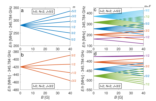
Figure 5: Energies, $E$, of the hyperfine-Zeeman levels of the $v=0$, $N=2$ state as function of magnetic-field strength, $B$, for a),b) the $I=0$ and c), d) the $I=2$ nuclear-spin species. The spin-rotation quantum number is $J=5/2$ in panels a) and c), and $J=3/2$ in panels b) and d). Color code for the different hyperfine states in c), d): $F=1/2$ in purple, $F=3/2$ in red, $F=5/2$ in blue, $F=7/2$ in green and $F=9/2$ in light blue. In panels a) and b), all Zeeman quantum numbers are shown while in panels c) and d) only the level with the highest value of the Zeeman quantum number ($m=F$) is indicated.

For the $I=2$ nuclear-spin species in the $N=2$ rotational state, the levels are further split by the hyperfine interaction which is dominated by the Fermi-contact ($H_{b_{F}}$) and dipolar ($H_{t}$) terms. Thus, the energy levels split into $F=9/2,...,1/2$ and $F=7/2,...,1/2$ for the $J=5/2$ (Fig. 5c) and $J=3/2$ Fig. 5d) spin-rotation manifolds, respectively. M1_S coupling is again dominant. For spin-rotation transitions, we found that $\Delta F=1$ components are prevalent, as can be seen in the spectrum displayed in Fig. 6. “Magic” transitions can be found at magnetic fields as low as few Gauss (e.g., the $|F=5/2,m=+1/2\rangle\rightarrow|F^{\prime}=7/2,m^{\prime}=-1/2\rangle$ at $\sim$756.3 MHz and $B=1.55$ G with second-order Zeeman-shifts as low as $\sim 8$ mHz/mG² (see Appendix D for a partial list of the strongest “magic” transitions below 70 G).

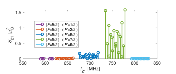
Figure 6: Strengths, $S_{21}$, of transitions between hyperfine components of the spin-rotation manifolds in the $X^{2}\Sigma_{g}^{+}$ ($v=0$, $N=2$) state of N${}_{2}^{+}$ as a function of the transition frequency ,$f_{21}$, at a magnetic-field strength of 10 G. The transitions shown are of the form $|N=2,J=3/2,I=2,F=5/2\rangle\rightarrow|N^{\prime}=2,J^{\prime}=5/2,I^{\prime}=2,F^{\prime}\rangle$.

An interesting effect in N${}_{2}^{+}$ as exemplified here with the $N=2$ manifold is the coupling between nuclear-spin states through the electric-quadrupole hyperfine interaction, $H_{eqQ}$, which mixes levels with even (or odd) total nuclear spin $I$. In ¹⁴N${}_{2}^{+}$, there is only a single para nuclear-spin state with $I=1$ such that only the ortho species with $I=0,2$ exhibit this coupling. This interaction results in avoided crossings of energy levels originating from the different ortho spin states. As an example, Fig. 7a shows such an avoided crossing between the $|F=3/2,m=-3/2\rangle$ states originating from the $I=0$ (red) and $I=2$ (blue) species. This avoided crossing occurs at a relatively low magnetic field of $\sim$54 G. Around the crossing point, the levels exhibit a strong mixing of the $I=0$ and $I=2$ basis states (see Fig. 7b). This magnetically enhanced nuclear-spin mixing is interesting as it opens up possibilities to manipulate the nuclear-spin configuration of the molecule on demand (see Fig. 12 and the accompanying discussion further below).

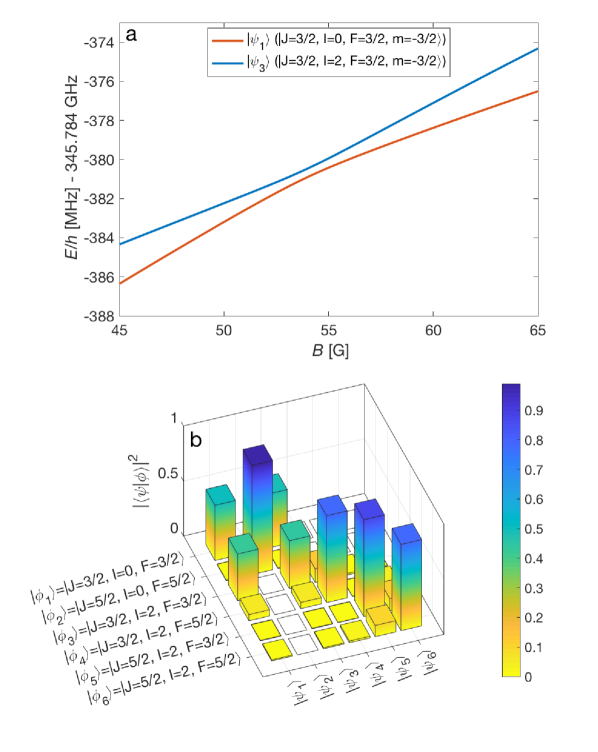
Figure 7: a) Adiabatic level energies, $E$, as a function of the magnetic field strength, $B$, showing an avoided crossing between two states originating from two different nuclear-spin states ($I=0,2$) in the $X^{2}\Sigma_{g}^{+}$(v=0, N=2) level. The states indicated in the legend represent the dominant contributions at zero magnetic field. b) Overlap of the eigenstates (Eq. 11) with the basis vectors (Eq. 3), $|\langle\phi_{i}|\psi_{k}\rangle|^{2}=|c_{i}^{k}|^{2}$, at a magnetic field of 54 G. Here, $|\langle\phi_{i}|\psi_{k}\rangle|^{2}\approx\delta_{ik}$ for zero magnetic field.

III.3 Rotational qubits

We now consider transitions from the rotational ground state $N=0$ to the second excited rotational state $N^{\prime}=2$ at frequencies around $\sim$345 GHz. The sensitivity of these transitions to the proton-to-electron mass ratio Hanneke et al. (2016) renders them interesting for testing a possible time variation of these fundamental constants as they are within the reach of stabilized THz sources Schiller et al. (2008).

In general, M1_S transition selection rules do not permit a change of rotational quantum numbers by $\Delta N=2$, but this mechanism must still be considered due to mixing of rotational states. In addition, the anisotropy of the electron-spin $g$-factor tensor allows for $\Delta N=2$ transitions through M1_aS coupling. We also consider electric-quadrupole (E2) transitions which also permit such a change in the rotational quantum number. In addition, E2 transitions permit changes in the angular-momentum-projection quantum number $\Delta m=\pm 2,\pm 1,0$. Thus, magnetic-dipole and electric-quadrupole rotational spectra will show different signatures as illustrated in Fig. 8a,b. For the $|J=1/2\rangle\rightarrow|J^{\prime}=3/2\rangle$ transitions, M1_aS coupling was found to be $\sim$3 orders of magnitude stronger than the E2 coupling while for the $|J=1/2\rangle\rightarrow|J^{\prime}=5/2\rangle$, it was only found to be about 1 order of magnitude stronger (Fig. 8a,b).

The $\Delta m=\pm 2$ and $\Delta J=2$ lines are allowed for E2 coupling opening up opportunities to exploit transitions between “stretched” states, e.g., $\left|J=1/2,m=\pm 1/2\right\rangle\rightarrow\left|J^{\prime}=5/2,m^{\prime}=\pm 5/2\right\rangle$ in the $I=0$ nuclear-spin isomer and $\left|F=5/2,m=\pm 5/2\right\rangle\rightarrow\left|F^{\prime}=9/2,m^{\prime}=\pm 9/2\right\rangle$ in the $I=2$ nuclear-spin isomer. These transitions show a very small linear dependence on the magnetic field due to cancellation of the major contribution from the isotropic Zeeman Hamiltonian (Eq. 7) in the ground and excited “stretched” states. The remaining susceptibility of these levels to magnetic field is attributed to the rotational dependence of the anisotropic (Eq. 10) and rotational (Eq. 8) Zeeman Hamiltonians. The isotropic term (Eq. 7) still has a small effect due to mixing of the rotational states. Thus, precise measurements of the magnetic dependence of these transitions can be used for an accurate determination of the anisotropic electron-spin and rotational $g$-factors.

The “stretched” transitions depend linearly on the magnetic field in the range considered here (up to 70 G) as can be seen in Fig. 8c. The frequencies of these transitions will change by $\Delta E/h=\Delta f\approx$475 mHz for magnetic field fluctuations of 1 mG. Therefore, they can be exploited for encoding THz qubits with coherence times of up to $1/\Delta f\approx 2$ s Saleh and Teich (2007) and for precision THz spectroscopy. The rotational spectrum of the $I=2$ nuclear-spin species also exhibits “magic” magnetic-field insensitive transitions with second-order shifts as low as $\sim 3$ mHz/mG² (Appendix D). Magnetic field fluctuations on the order of $\sim 1$ mG still permit qubits with Zeeman-limited coherence times of up to $1/\Delta f\approx 5$ min.

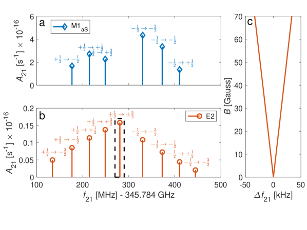
Figure 8: Spectrum of Zeeman components of the spin-rotational transition $|N=0,J=1/2\rangle\rightarrow|N^{\prime}=2,J^{\prime}=5/2\rangle$ for the $I=0$ isomer. The intensities of the transitions are given in the form of Einstein $A$ coefficients (Eqs. 23,22) for comparison of a) M1_aS coupling with b) E2 coupling. The magnetic field was assumed to be 70 G. Labels indicate the Zeeman components of the transitions. c) Magnification of the dashed rectangle in b) showing the stretched transitions, $|J=1/2,m=\pm 1/2\rangle\rightarrow|J^{\prime}=5/2,m^{\prime}=\pm 5/2\rangle$, which show a very small dependence on the magnetic field and are only separated by 66.5 kHz at 70 G. The frequency axis in c) is referenced to the field-free line positions.

In Fig. 9, the hyperfine components of the transition $|N=0,J=1/2,F=5/2\rangle\rightarrow|N^{\prime}=2,J^{\prime}=5/2,F^{\prime}\rangle$ in the $I=2$ nuclear-spin state due to M1 and E2 coupling are shown. The M1_S rotational transitions are allowed by rotational mixing induced by the dipolar hyperfine interaction, $H_{t}$. The strongest M1_S lines are on-par with the strongest M1_aS lines and are up to two order of magnitude stronger than the E2 lines. However, in some cases the strengths for both types of transitions are similar and in other cases, only E2 transitions are allowed due to quadrupole selections rules. Thus, one should consider both types of transitions when analyzing the molecular spectrum. To directly compare the strength of both types of couplings with Eq. 12, we calculated the relevant Einstein $A$ coefficients using Eq. 22 and Eq. 23.

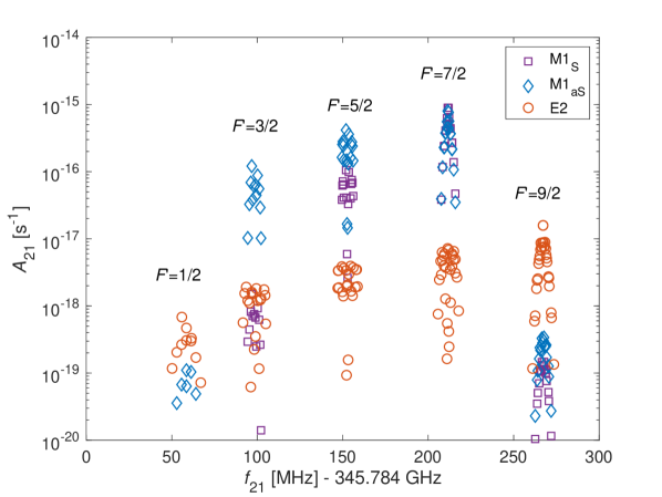
Figure 9: Einstein $A$ coefficients of hyperfine-Zeeman components of the spin-rotational transition $|N=0,J=1/2,F=5/2\rangle\rightarrow|N^{\prime}=2,J^{\prime}=5/2,F^{\prime}\rangle$ of the $I=2$ nuclear-spin species. Transitions due to M1_S, M1_aS and E2 are indicated by purple squares, blue diamonds and red circles. The magnetic field was set to 5 G.

III.4 Rovibrational qubits

Dipole-forbidden rovibrational lines in N${}_{2}^{+}$ were first observed by Germann et al. Germann et al. (2014). Vibrational transitions are promising for tests of a possible temporal variation of the proton-to-electron mass ratio because of their sensitivity to these constants. Also, they benefit from higher transition frequencies than rotational lines and thus allow for a better relative precision Kajita et al. (2014). Fig. 10 shows the O($N$), Q($N$) and S($N$) branches of the fundamental vibrational spectrum, i.e., transitions with $|v=0,N\rangle\rightarrow|v^{\prime}=1,N^{\prime}=N+(-2,0,+2)\rangle$ and $N=0,2,4$ and for the two ortho nuclear-spin species.

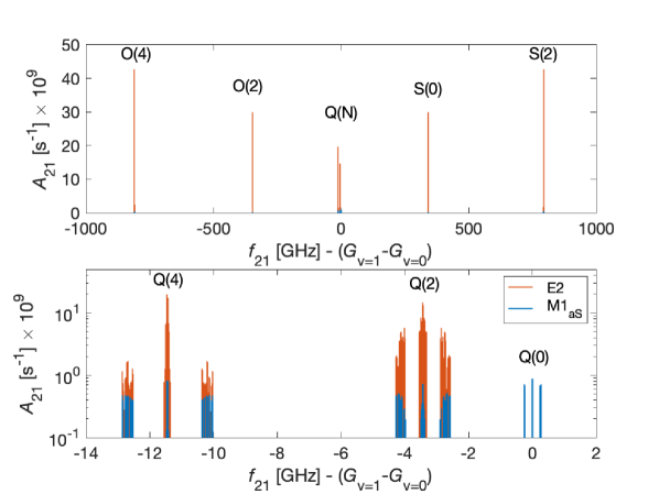
Figure 10: Einstein $A$ coefficients of E2 (red lines) and M1_aS (blue lines) transitions of the O($N$=2,4), Q($N$=0,2,4) and S($N$=0,2) branches of the fundamental vibrational transition $|v=0,N\rangle\rightarrow|v^{\prime}=1,N^{\prime}\rangle$. The magnetic field was assumed to be 5 G. The lower panel shows a magnification of the spectrum in the region of the Q branch.

Transitions within the Q(0) manifold, $\left|v=0,N=0\right\rangle\rightarrow\left|v^{\prime}=1,N^{\prime}=0\right\rangle$, are usually considered to be forbidden for single photon excitation within a $\Sigma$ electronic state Kajita et al. (2014). E2 selection rules forbid transitions from $N=0$ to $N^{\prime}=0$. However, the anisotropic electron-spin interaction (Eq. 10) permits $N=0$ to $N^{\prime}=0$ transitions and it varies considerably with the internuclear distance (Eq. 20). This leads to the appearance of Q(0) lines in the spectrum which, to the best of our knowledge, were so far not considered for the present vibrational spectrum.

In Fig. 11, components of the Q(0) transition, i.e. $|v=0,N=0,J=1/2\rangle\rightarrow|v^{\prime}=1,N^{\prime}=0,J^{\prime}=1/2\rangle$, of both the $I=0$ and $I=2$ species is shown. For both nuclear-spin configurations, the “stretched” transitions, i.e $|J=1/2,m=\pm 1/2\rangle\rightarrow|J^{\prime}=1/2,m^{\prime}=\pm 1/2\rangle$ and $|F=5/2,m=\pm 5/2\rangle\rightarrow|F^{\prime}=5/2,m^{\prime}=\pm 5/2\rangle$ are allowed by M1_aS coupling and show very small linear Zeeman shifts of $\Delta g_{l}/3\approx 9.3$ mHz/mG. This dependency is $\sim 50$ times smaller than for transitions between “stretched” states in the S(0) ($|N=0\rangle\rightarrow|N^{\prime}=2\rangle$) manifold. Precise measurements of the magnetic dependence of these transitions constitute a direct measurement of the anisotropy of the electron-spin $g$-factor tensor.

The Q(0) spectrum also exhibits “magic“ transitions for the $I=2$ species (indicated by black crosses in Fig. 11) at relatively low magnetic fields of a few 10 G. The second-order Zeeman susceptibility of these transitions is $\sim 16$ mHz/mG². Note that there are no “magic” transitions for the $I=0$ nuclear-spin configuration when driving a transition from the rotational ground state, $N=0$. This is due to the linear Zeeman shifts of the rotational ground state at the magnetic field values considered here (see Fig. 2a green lines).

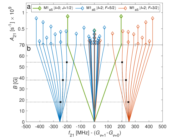
Figure 11: a) Einstein $A$ coefficients b) and line positions as function of magnetic-field strength, $B$, of hyperfine-Zeeman components of the Q(0) line of the fundamental vibrational transition $|v=0,N=0\rangle\rightarrow|v^{\prime}=1,N^{\prime}=0\rangle$. Black crosses and dotted lines indicate positions of “magic” magnetic-field transitions.

We now turn to discuss S(0) transitions, i.e. $\left|v=0,N=0\right\rangle\rightarrow\left|v^{\prime}=1,N^{\prime}=2\right\rangle$. The S(0) spectrum is predicted to be $\sim 30$ times stronger (see Fig. 10 red lines) than the the Q(0) spectrum due to E2 transitions (Eq. 20). The second largest contribution to the S(0) spectrum is due to M1_aS coupling (Fig. 10 blue lines). All other coupling mechanisms were found to be more than 5 orders of magnitude smaller. Q(2) transitions, $\left|v=0,N=2\right\rangle\rightarrow\left|v^{\prime}=1,N^{\prime}=2\right\rangle$, are also dominated by E2 coupling.

The S(0) spectrum is predicted to exhibit “magic” transitions at low magnetic fields of a few Gauss and with second-order Zeeman susceptibilities as low as $\sim$ 1 mHz/mG² (see Appendix D). With magnetic field fluctuations on the order of $\sim 1$ mG, they can be used for encoding vibrational qubits with coherence times of up to $\approx 15$ min. This corresponds to a relative Zeeman shift of $\Delta E/E\approx 1\times 10^{-17}$ without any active or passive magnetic field stabilization. The S(0) spectrum also features “streched” transitions that have a low linear Zeeman shift of $\sim$480 mHz/mG.

The S(0) transitions at 4.574 $\mu$m with $A\approx 3\times 10^{-8}$ Hz can be driven using commercial quantum-cascade lasers as demonstrated in Ref. Germann et al. (2014). With typical values for the laser power of 100 mW and a $1/e$ beam radius of 50 $\mu$m at the position of the molecule, Rabi frequencies Leibfried et al. (2003) of $\Omega\sim(2\pi)$10 kHz are estimated yielding $\pi$-pulse times of $t_{\pi}\sim$50 $\mu$s thus enabling an efficient coherent manipulation of the rovibrational levels of the molecule. For the Q(0) transitions, $A\approx 4\times 10^{-10}$ Hz. With the same laser parameters, $\Omega\sim(2\pi)$0.5 kHz and $t_{\pi}\sim$1 ms are estimated.

The $|v^{\prime}=1,N^{\prime}=2\rangle$ rotational manifold of the first excited vibrational state exhibits avoided crossings between levels of the two ortho-nuclear-spin species as illustrated in Fig. 12. The mixing is again induced by the quadrupole hyperfine interaction, $H_{eqQ}$. At a magnetic field of $\sim$25.8 G, the states labeled $|\psi^{\prime}_{0,2}\rangle$ in Fig. 12 are composed of a 50-50 mixture of the $|I^{\prime}=2,F^{\prime}=3/2,m^{\prime}=-3/2\rangle$ and $|I^{\prime}=0,J^{\prime}=3/2,m^{\prime}=-3/2\rangle$ basis states. This opens up the possibility of coupling two distinct molecular states of different nuclear-spin character, for instance the $|\psi_{2}\rangle=|I=2,F=5/2,m=1/2\rangle$ and $|\psi_{0}\rangle=|I=0,J=1/2,m=1/2\rangle$ in the rovibrational ground state, $v=0,N=0$. These states show negligible nuclear-spin mixing. Fig. 12 illustrates how these two states in the vibrational ground state can be interconverted by excitation and deexcitation to the mixed states $|\psi^{\prime}_{0,2}\rangle$ in $v=1$. Alternatively, interconversion of the nuclear-spin states can be achieved by populating one of the mixed state in $v=1$ and appropriately tuning the magnetic field across the crossing region.

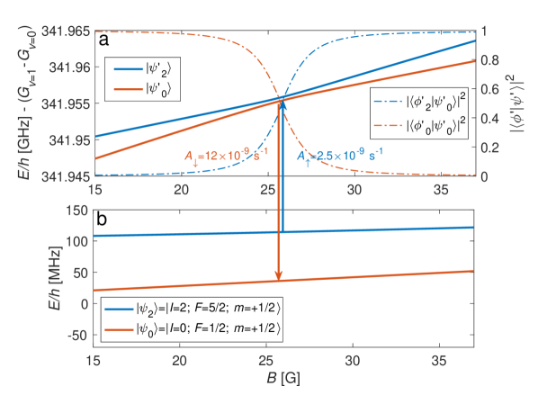
Figure 12: a) Adiabatic level energies, $E$, as a function of the magnetic field, $B$, showing an avoided crossing between two states originating from $|I^{\prime}=2,F^{\prime}=3/2,m^{\prime}=-3/2\rangle$ ($|\psi^{\prime}_{2}\rangle$, blue line) and $|I^{\prime}=0,J^{\prime}=3/2,m^{\prime}=-3/2\rangle$ ($|\psi^{\prime}_{0}\rangle$, red line) in the $v^{\prime}=1,N^{\prime}=2$ rovibrational-state manifold. The dashed-dotted lines indicate the degree of mixing, $\left|\langle\phi^{\prime}_{j}|\psi^{\prime}_{0}\rangle\right|^{2}$, where $|\phi^{\prime}_{j}\rangle$ are the basis states ($j=0,2$) describing $|\psi^{\prime}_{j}\rangle$ at low magnetic fields. At a magnetic-field strength of $\sim$25.8 G, a 50-50 mixture of the $I=0$ and $I=2$ states is predicted. b) Levels of the $I=2$ (blue) and the $I=0$ (red) nuclear-spin configurations in the rovibrational ground state are coupled by a resonant two-photon process (arrows). The coupling is performed through S(0) transitions to one of the highly mixed nuclear-spin states. The coupling strengths to the $|\psi^{\prime}_{0}\rangle$ state in the form of the Einstein $A$ coefficients for $\Delta m=-2$ transitions are given in the plot.

IV Summary and conclusions

In this paper, we presented a theoretical study of dipole-forbidden spectroscopic transitions in N${}_{2}^{+}$ considering the complete hyperfine, rovibrational and Zeeman level structure. We identified magnetic-field insensitive transitions which are promising for encoding qubits because of their excellent coherence properties and for clock operation because of their weak dependence on magnetic fields. We calculated the strengths of magnetic-dipole and electric-quadrupole allowed spectroscopic transitions showing the importance of both in the radiofrequency, microwave and infrared spectrum of the nitrogen molecular ion. We found that pure vibrational transitions, Q(0), are allowed by M1 coupling induced by the anisotropic spin-magnetic field interaction. These transitions, which benefit from the lowest systematic shifts for clock operation, were not considered in the single-photon spectrum of N${}_{2}^{+}$ so far. Finally, we showed that the electric-quadrupole hyperfine interaction causes avoided crossings between states of the two ortho nuclear-spin configurations of nitrogen. This magnetically enhanced nuclear-spin mixing opens the possibility to coherently transmute the the nuclear-spin state on demand.

It is instructive to make a quantitative comparison between the magnetic insensitivity of clock transitions embedded in N${}_{2}^{+}$ to other clock systems, e.g., Al⁺ quantum-logic clocks which currently exhibit among the lowest systematic uncertainties Brewer et al. (2019a). The Al⁺ clock is based on the ¹S${}_{0}\leftrightarrow^{3}$P₀ electronic transition which is first-order magnetically sensitive due to the nuclear spin, $I=5/2$, of ²⁷Al⁺. By averaging two stretched Zeeman transitions, the first-order shift is canceled, and the clock only depends on second-order Zeeman shifts Brewer et al. (2019b). This averaging technique is not an option for qubit applications. The second-order sensitivity of Al⁺, $\sim 7.2\times 10^{-4}$ mHz/mG², is five orders of magnitude smaller than the sensitivity of N${}_{2}^{+}$ “magic” transitions analysed here. However, since the Al⁺ clock works at a finite magnetic field of 1.2 G Brewer et al. (2019a), the clock transition acquires an effective first-order sensitivity of $\sim 1.7$ mHz/mG. This first-order sensitivity is five times smaller than that of the Q(0) “streched” transitions in N${}_{2}^{+}$. However, for the “magic” transitions in N${}_{2}^{+}$, which have a vanishing first-order sensitivity, the magnetic-field sensitivity breaks even with the Al⁺ clock transition at a fluctuating magnetic field value of $\sim 0.1$ mG which is a typical value for a system with actively stabilized magnetic field. Below this value, the N${}_{2}^{+}$ “magic” transitions are less sensitive than the Al⁺ clock while above they are more sensitive to magnetic field fluctuations.

Appendix

Appendix A Electric-field induced systematic shifts

In the main text, we have considered the usefulness of different types of spectroscopic transitions for clock applications and as qubits in terms of their sensitivity to magnetic fields which causes the dominant systematic shifts in N${}_{2}^{+}$. In addition, viable clock candidates should also have low susceptibilities to electric fields. For completeness, we consider here the AC-Stark and electric quadrupole shifts, complementing the discussion in Ref. Kajita et al. (2014).

A.1 Stark shifts

In a homonuclear diatomic molecule, there is no electric-dipole coupling between rovibrational states and the first-order Stark shift vanishes. There is, however, dipole coupling to excited electronic states. The AC-Stark shift of state $j$ is given by,

$$\Delta E_{j}=-\frac{1}{2}\alpha_{j}(\omega)E_{0}^{2},$$ (24)

where $E_{0}$ is the electric field amplitude at frequency $\omega$ and $\alpha_{j}(\omega)$ is the polarizability given by,

$$\alpha_{j}(\omega)=\sum\limits_{k}\frac{|\langle k|\mathbf{\mu}|j\rangle|^{2}}{\hbar}\frac{\omega_{jk}}{\omega^{2}-\omega_{jk}^{2}}.$$ (25)

Here, the summation runs over all states of the molecule, $k$, with non-vanishing dipole matrix element, $\langle k|\mathbf{\mu}|j\rangle$, and transition angular frequency, $\omega_{jk}$. Data on excited electronic states of N${}_{2}^{+}$ can be found in the literature, e.g., Ref. Lofthus and Krupenie (1977). The AC-Stark-shift-induced differential shift of the transition frequency between two levels $j$ and $i$ is then given by $h\Delta f_{AC}=\Delta E_{j}-\Delta E_{i}$.

Different types of AC-Stark shifts contribute to the present problem. The AC-Stark shift from the RF drive of an ion trap with frequency $\omega\approx(2\pi)20$ MHz can be estimated in the limit $\omega\rightarrow 0$ in Eq. (25). For vibrational transitions with $f\approx 65.2$ THz, one obtains a relative shift of $\Delta f_{AC}/(fE_{0}^{2})=7\times 10^{-24}$ (m/V)². Typically, the electric field amplitude vanishes at the position of the ions in a Paul trap. However, trap imperfections can lead to a non-zero electric-field amplitude. These fields will cause a relative shift of $1.26\times 10^{-18}$ at a field amplitude of $300$ V/m for the fundamental vibrational transition. It should be noted that such a field amplitude is excessive for an ion in a typical ion trap built for quantum-logic experiments. For other classes of transitions, e.g., hyperfine or rotational excitations, the corresponding shift is smaller as the energy spacing decreases and the cancellation of the AC-Stark shift between the upper and the lower state is more significant.

The AC-Stark shift induced by ambient blackbody radiation can also be estimated in the limit of $\omega\rightarrow 0$ because the maximum of the thermal spectral energy density at a temperature of 300 K is situated around 31 THz which is small compared to the frequencies of electronic transitions from the vibrational ground-state. The time-averaged value of the quadratic electric-field amplitude of a 300 K radiator is $E_{0}^{2}/2=\langle E_{0}^{2}\rangle\approx(831.9$ V/m)² Riehle (2005) yielding a relative shift of $\Delta f_{AC}/f=1.0\cdot 10^{-17}$ for vibrational transitions. Transitions within a vibrational state will have smaller shifts due to cancellation between the upper and lower levels. The N${}_{2}^{+}$ molecular clock is therefore suitable for operation in a room-temperature environment.

AC-Stark shifts from the probe laser can be eliminated by using the Hyper-Ramsey spectroscopic method Yudin et al. (2010) or through a balanced Raman scheme Sanner et al. (2018). In a Rabi- or Ramsey-type clock experiment, the laser power is reduced in order to minimize power broadening. In order to obtain a Rabi frequency of $\Omega\sim(2\pi)1$ Hz on the S(0) branch of the fundamental vibrational transition, 1 nW of laser power focused to a beam radius of $50~{}\mu$m are required. The intensity is thus $I=0.26$ W/m² corresponding to an electric field of $13.9$ V/m. The AC-Stark shift obtained from Eq. (24) is then $\Delta f_{AC}/f=8.9\cdot 10^{-22}$. With a laser power more suitable for driving qubits of $\sim 100$ mW, the intensity is $I=2.55\cdot 10^{7}$ W/m² and an AC-Stark shift of $5.8$ Hz or $\Delta f_{AC}/f=8.9\times 10^{-14}$ is obtained.

A.2 Electric-quadrupole shift

The matrix element in Eq. 18 that was used to obtain the electric quadrupole transition moment can also be used for estimating the quadrupole shift caused by static-field gradients prevalent in an ion trap. For the present purpose, the permanent moments $R(0,0)\approx 1.86$ $ea_{0}^{2}$ for $v=0$ and $R(1,1)\approx 1.89$ $ea_{0}^{2}$ for $v=1$ Bruna and Grein (2004) were assumed in Eq. 18. Furthermore, we assumed $p=0$ to describe a static field gradient along the trap axis. The first-order energy correction due to the quadrupole shift is then given by Bakalov and Schiller (2014),

$$\Delta E_{j}=-\frac{1}{3}\frac{dE}{dz}\langle\phi_{i}|\mathbf{Q}|\phi_{j}\rangle.$$ (26)

A typical field gradient, $dE/dz$, in an ion trap is $\sim 10^{7}$ V/m². From the matrix elements in Eq.18, we see that the quadrupole shift vanishes for all states in the rotational ground state, $N=0$, as is also apparent by the selection rules for E2 transitions. Further, for any state with $F=0$ or $F=1/2$, the shift also vanishes. For other states in $v=0,1$ and $N=0,2,4$, the matrix element ranges between $10^{-3}-10^{-1}R(v,v)$ corresponding to an absolute quadrupole shift between $0.013-1.3$ Hz.

All the Zeeman-and hyperfine transitions in $N=0$ are therefore immune to electric-quadrupole shifts to first order. Rotational transitions of the form $N=0\rightarrow(N^{\prime}=2$, $F=1/2)$, among which several “magic” transitions were identified (see Appendix D), are also not affected by this shift, as is the Q(0) branch of vibrational transitions. The Q(0) transitions of the $I=0$ nuclear-spin configuration are therefore especially suitable for clock operation because they are immune from the quadrupole shift and feature stretched-state transitions which have a low susceptibility to magnetic fields. Q(2) transitions can also be chosen with $F=F^{\prime}=1/2$ such that the quadrupole shift cancels. For S(0) transitions, the quadrupole shift vanishes in the lower states $N=0$ and the upper state can be chosen as $F^{\prime}=1/2$.

The differential shift of the fine-structure transitions with $\Delta J=1$ within the $N=2$ manifold was calculated for the “magic” transitions listed in Appendix D. The differential shift ranges between $0.38-1.86$ Hz for the “magic” transitions with the exception of $|J=3/2,I=2,F=7/2,M_{F}=-1/2\rangle\rightarrow|J=5/2,I=2,F=9/2,M_{F}=-3/2\rangle$ for which an accidental cancellation leads to a vanishing shift. Therefore, suitable clock transitions with a low sensitivity to magnetic fields and vanishing quadrupole shifts were identified in every class of transitions examined in this paper.

Appendix B The effective hyperfine Hamiltonian

The effective hyperfine-interaction Hamiltonian takes the form,

$$H_{hfs}=H_{b_{F}}+H_{t}+H_{eqQ}+H_{c_{I}}.$$ (27)

The individual terms in $H_{hfs}$ and their matrix elements have been discussed in Ref. Mansour et al. (1991) and are reproduced here for convenience. $H_{b_{F}}$ represents the Fermi-contact interaction which has off-diagonal matrix elements in $J$,

$$\langle v^{\prime},N^{\prime},S^{\prime},J^{\prime},I^{\prime},F^{\prime},m^{\prime}|H_{b_{F}}|v,N,S,J,I,F,m\rangle=b_{Fv}\delta_{vv^{\prime}}\delta_{NN^{\prime}}\delta_{SS^{\prime}}\delta_{II^{\prime}}\delta_{FF^{\prime}}\delta_{mm^{\prime}}(-1)^{F+I+J^{\prime}+J+N+S+1}$$ (28)

$$\times\sqrt{I(I+1)(2I+1)S(S+1)(2S+1)(2J+1)(2J^{\prime}+1)}\begin{Bmatrix}I&J^{\prime}&F\\ J&I&1\end{Bmatrix}\begin{Bmatrix}S&J^{\prime}&N\\ J&S&1\end{Bmatrix},$$

$H_{t}$ is the dipolar hyperfine interaction with off-diagonal matrix elements in $N$ and $J$,

$$\langle v^{\prime},N^{\prime},S^{\prime},J^{\prime},I^{\prime},F^{\prime},m^{\prime}|H_{t}|v,N,S,J,I,F,m\rangle=t_{v,N}\delta_{vv^{\prime}}\delta_{SS^{\prime}}\delta_{II^{\prime}}\delta_{FF^{\prime}}\delta_{mm^{\prime}}(-1)^{J+I+F+N^{\prime}+1}$$ (29)

$$\times\sqrt{30I(I+1)(2I+1)S(S+1)(2S+1)(2J+1)(2J^{\prime}+1)(2N+1)(2N^{\prime}+1)}$$

$$\times\begin{Bmatrix}I&J^{\prime}&F\\ J&I&1\end{Bmatrix}\begin{Bmatrix}N^{\prime}&N&2\\ S&S&1\\ J^{\prime}&J&1\end{Bmatrix}\begin{pmatrix}N^{\prime}&2&N\\ 0&0&0\end{pmatrix},$$

where $t_{v,N}=t_{v}+t_{Dv}N(N+1)$, $H_{eqQ}$ is the electric-quadrupole hyperfine interaction with off-diagonal matrix elements in $N$, $J$ and $I$,

$$\langle v^{\prime},N^{\prime},S^{\prime},J^{\prime},I^{\prime},F^{\prime},m^{\prime}|H_{eqQ}|v,N,S,J,I,F,m\rangle=\frac{eqQ_{v}}{2}\delta_{vv^{\prime}}\delta_{SS^{\prime}}\delta_{FF^{\prime}}\delta_{mm^{\prime}}$$ (30)

$$\times\frac{(-1)^{I}+(-1)^{I^{\prime}}}{2}(-1)^{F+2J+I^{\prime}+2I_{1}+S+2N^{\prime}}$$

$$\times\sqrt{(2I+1)(2I^{\prime}+1)(2J+1)(2J^{\prime}+1)(2N+1)(2N^{\prime}+1)}$$

$$\times\begin{Bmatrix}I^{\prime}&2&I\\ J&F&J^{\prime}\end{Bmatrix}\begin{Bmatrix}I_{1}&2&I_{1}\\ I&I_{1}&I^{\prime}\end{Bmatrix}\begin{Bmatrix}N^{\prime}&2&N\\ J&S&J^{\prime}\end{Bmatrix}\begin{pmatrix}N^{\prime}&2&N\\ 0&0&0\end{pmatrix}\begin{pmatrix}I_{1}&2&I_{1}\\ -I_{1}&0&I_{1}\end{pmatrix}^{-1},$$

where $I_{1}=1$ is the nuclear spin of a ¹⁴N atom, and $H_{c_{I}}$ is the magnetic nuclear spin-rotation interaction which mixes different $J$ quantum numbers,

$$\langle v^{\prime},N^{\prime},S^{\prime},J^{\prime},I^{\prime},F^{\prime},m^{\prime}|H_{c_{I}}|v,N,S,J,I,F,m\rangle=c_{I}\delta_{vv^{\prime}}\delta_{NN^{\prime}}\delta_{SS^{\prime}}\delta_{II^{\prime}}\delta_{FF^{\prime}}\delta_{mm^{\prime}}(-1)^{F+I+J^{\prime}+J+N+S+1}$$ (31)

$$\times\sqrt{I(I+1)(2I+1)N(N+1)(2N+1)(2J+1)(2J^{\prime}+1)}\begin{Bmatrix}J&1&J^{\prime}\\ I&F&I\end{Bmatrix}\begin{Bmatrix}N&1&N\\ J^{\prime}&S&J\end{Bmatrix}.$$

All effective coupling constants are given in Table 1.

Appendix C Vibrational mixing

The rovibrational mixing was estimated in the same way as in Refs. Balasubramanian et al. (1992, 1994), i.e., as a result of the dependence of the rotational constant, $B$, on the bond length, $R$, within the harmonic approximation for the vibration. The rotational constant, $B(R)\propto R^{-2}$, was expanded in a Taylor series to first order around the equilibrium internuclear distance $R=R_{e}$,

$$B(R)=B_{e}\left[1-2\hat{\xi}+O(\hat{\xi}^{2})\right].$$ (32)

Here, $\hat{\xi}=(\hat{R}-R_{e})/R_{e}$ and $B_{e}$ is the equilibrium rotational constant. The zero-order term corresponds to the rigid-rotor rotational Hamiltonian whereas the linear term in $\hat{\xi}$ causes the rovibrational interaction.

Inserting Eq. 32 in the rotational Hamiltonian, $B(R)\hat{N}^{2},$ the rigid-rotor Hamiltonian, $B_{e}\hat{N}^{2}$, and the rotation-vibration coupling Hamiltonian to first order,

$$\mathscrsfs{H}_{ro-vib}=-2B_{e}\hat{\xi}\hat{N}^{2}.$$ (33)

are obtained. $\hat{\xi}$ is further expressed in terms of creation ($\hat{a}^{\dagger}$) and annihilation ($\hat{a}$) operators of an harmonic oscillator,

$$\hat{\xi}=\sqrt{\frac{B_{e}}{\omega_{e}}}(\hat{a}^{\dagger}+\hat{a}),$$ (34)

which results in the matrix elements,

$$\langle v^{\prime},N^{\prime}|\mathscrsfs{H}_{\text{ro-vib}}|v,N\rangle=-2B_{e}\sqrt{\frac{B_{e}}{\omega_{e}}}\delta_{NN^{\prime}}$$ (35)

$$\times N(N+1)\left(\sqrt{v+1}\delta_{v^{\prime},v+1}+\sqrt{v}\delta_{v^{\prime},v-1}\right).$$

Here, $\omega_{e}$ is the harmonic vibration frequency (expressed in the same units as $B_{e}$).

The combined vibrational and rotational Hamiltonians, $\mathscrsfs{H}_{vib}=G_{v}$ and $\mathscrsfs{H}_{rot}=B_{e}\hat{N}^{2}$, respectively, were diagonalized including the rovibrational interaction $\mathscrsfs{H}_{ro-vib}$ numerically using the $v=0,1,2,3,4$ vibrational and $N=0,2,4,6,8,10$ rotational states as a basis set to obtain the mixing coefficients. In this treatment, we found $\sum\limits_{ij}c_{i}c_{j}R(v=0,v=1)\sim 5\times 10^{-6}\mu_{p}$ in $N=2$ according to Eq. 20. For E2 transitions, this corresponds to transition moment of $\sim 10^{-5}~{}ea_{0}^{2}$. The second term in Eq. 20, however, leads to a much stronger transition moment of $\sim 10^{-1}~{}ea_{0}^{2}$. Therefore, the effect of ro-vibrational mixing in the calculation of the transition moments for low-lying rotational states can be neglected.

Appendix D “Magic” magnetic-field-insensitive transitions

Table 2: Partial list of the strongest “magic” magnetic-field insensitive transitions within the hyperfine, fine, rotational and vibrational manifolds below 70 G. The labels $\left|v,N,S,J,I,F,m\right\rangle$ correspond to those basis states which exhibit the largest overlap with with the true molecular eigenstates. For each transition, the “magic” magnetic-field strength, $B$, the Einstein $A$ coefficient, the transition frequency, $f-f_{0}$, and the second-order magnetic-field dependence, $a$, of the transition are indicated. The dominant coupling mechanism (M1_S, M1_aS or E2) is also listed for each type of transition. The transition frequencies are given with respect to a reference frequency, $f_{0}$, defined as follows: $f_{0}=0$ for pure hyperfine and fine-structure transitions, $f_{0}=B_{0}\times 6-D_{0}\times 6^{2}\approx 345^{\prime}784.31$ MHz for rotational transitions, $f_{0}=G_{1}-G_{0}\approx 65^{\prime}197^{\prime}244.88$ MHz for Q(0) rovibrational transitions, and $f_{0}=G_{1}-G_{0}+B_{1}\times 6-D_{1}\times 6^{2}\approx 65^{\prime}539^{\prime}595.50$ MHz for S(0) rovibrational transitions.

Hyperfine transitions: ($I=2$) M1S	$|v=0,N=0\rangle\rightarrow|v^{\prime}=0,N^{\prime}=0\rangle$	$B$ [G]	$A$ [s-1]	$f-f_{0}$ [MHz]	$a$ [mHz/mG2]
$|J=1/2,I=2,F=3/2,m=-3/2\rangle\rightarrow$	$|J=1/2,I=2,F=5/2,m=-3/2\rangle$	54.85	8.6$\times 10^{-18}$	204.80	19.1
$|J=1/2,I=2,F=3/2,m=-1/2\rangle\rightarrow$	$|J=1/2,I=2,F=5/2,m=-3/2\rangle$	38.40	6.1$\times 10^{-18}$	233.51	16.1
$|J=1/2,I=2,F=3/2,m=-3/2\rangle\rightarrow$	$|J=1/2,I=2,F=5/2,m=-1/2\rangle$	38.42	6.1$\times 10^{-18}$	233.48	16.1
$|J=1/2,I=2,F=3/2,m=-1/2\rangle\rightarrow$	$|J=1/2,I=2,F=5/2,m=-1/2\rangle$	18.28	1.6$\times 10^{-17}$	250.83	15.6
Fine-structure transitions: ($I=0,2$) M1S	$|v=0,N=2\rangle\rightarrow|v^{\prime}=0,N^{\prime}=2\rangle$	$B$ [G]	$A$ [s-1]	$f-f_{0}$ [MHz]	$a$ [mHz/mG2]
$|J=3/2,I=0,F=3/2,m=-1/2\rangle\rightarrow$	$|J=5/2,I=0,F=5/2,m=-1/2\rangle$	49.20	3.1$\times 10^{-16}$	686.52	8.9
$|J=3/2,I=2,F=3/2,m=-1/2\rangle\rightarrow$	$|J=5/2,I=2,F=5/2,m=-1/2\rangle$	17.15	2.2$\times 10^{-16}$	656.74	12.0
$|J=3/2,I=2,F=3/2,m=1/2\rangle\rightarrow$	$|J=5/2,I=2,F=5/2,m=-1/2\rangle$	3.81	1.0$\times 10^{-16}$	660.16	10.5
$|J=3/2,I=2,F=5/2,m=-1/2\rangle\rightarrow$	$|J=5/2,I=2,F=7/2,m=-3/2\rangle$	48.30	1.9$\times 10^{-16}$	738.06	8.0
$|J=3/2,I=2,F=5/2,m=-3/2\rangle\rightarrow$	$|J=5/2,I=2,F=7/2,m=-1/2\rangle$	48.72	1.6$\times 10^{-16}$	739.40	7.0
$|J=3/2,I=2,F=5/2,m=-1/2\rangle\rightarrow$	$|J=5/2,I=2,F=7/2,m=-1/2\rangle$	22.31	3.9$\times 10^{-16}$	752.31	8.2
$|J=3/2,I=2,F=5/2,m=1/2\rangle\rightarrow$	$|J=5/2,I=2,F=7/2,m=-1/2\rangle$	1.55	1.9$\times 10^{-16}$	756.33	7.9
$|J=3/2,I=2,F=7/2,m=-1/2\rangle\rightarrow$	$|J=5/2,I=2,F=9/2,m=-3/2\rangle$	49.84	2.8$\times 10^{-16}$	832.14	6.3
$|J=3/2,I=2,F=7/2,m=-3/2\rangle\rightarrow$	$|J=5/2,I=2,F=9/2,m=-1/2\rangle$	49.39	2.7$\times 10^{-16}$	832.67	6.2
$|J=3/2,I=2,F=7/2,m=-1/2\rangle\rightarrow$	$|J=5/2,I=2,F=9/2,m=-1/2\rangle$	24.06	5.9$\times 10^{-16}$	843.94	6.3
Rotational transitions: ($I=2$) M1aS	$|v=0,N=0\rangle\rightarrow|v^{\prime}=0,N^{\prime}=2\rangle$	$B$ [G]	$A$ [s-1]	$f-f_{0}$ [MHz]	$a$ [mHz/mG2]
$|J=1/2,I=2,F=3/2,m=-3/2\rangle\rightarrow$	$|J=3/2,I=2,F=1/2,m=-1/2\rangle$	45.57	2.2$\times 10^{-15}$	-244.08	9.4
$|J=1/2,I=2,F=3/2,m=-1/2\rangle\rightarrow$	$|J=3/2,I=2,F=1/2,m=-1/2\rangle$	15.80	9.3$\times 10^{-15}$	-225.74	12.3
$|J=1/2,I=2,F=3/2,m=-1/2\rangle\rightarrow$	$|J=3/2,I=2,F=1/2,m=1/2\rangle$	9.37	2.7$\times 10^{-15}$	-223.57	9.3
$|J=1/2,I=2,F=3/2,m=-3/2\rangle\rightarrow$	$|J=3/2,I=2,F=3/2,m=-3/2\rangle$	29.85	9.8$\times 10^{-15}$	-257.50	7.3
$|J=1/2,I=2,F=3/2,m=-1/2\rangle\rightarrow$	$|J=3/2,I=2,F=3/2,m=-1/2\rangle$	36.99	1.2$\times 10^{-15}$	-254.73	3.8
$|J=1/2,I=2,F=5/2,m=-3/2\rangle\rightarrow$	$|J=3/2,I=2,F=3/2,m=-1/2\rangle$	38.86	1.4$\times 10^{-15}$	-488.22	-12.1
$|J=1/2,I=2,F=5/2,m=-1/2\rangle\rightarrow$	$|J=3/2,I=2,F=3/2,m=-1/2\rangle$	15.30	1.9$\times 10^{-15}$	-504.42	-14.9
$|J=1/2,I=2,F=3/2,m=-1/2\rangle\rightarrow$	$|J=3/2,I=2,F=3/2,m=1/2\rangle$	48.51	7.4$\times 10^{-15}$	-264.22	5.3
$|J=1/2,I=2,F=3/2,m=1/2\rangle\rightarrow$	$|J=3/2,I=2,F=3/2,m=3/2\rangle$	17.64	5.9$\times 10^{-15}$	-253.71	5.4
$|J=1/2,I=2,F=3/2,m=-3/2\rangle\rightarrow$	$|J=3/2,I=2,F=5/2,m=-3/2\rangle$	44.15	7.7$\times 10^{-15}$	-297.86	5.9
$|J=1/2,I=2,F=5/2,m=-3/2\rangle\rightarrow$	$|J=3/2,I=2,F=5/2,m=-3/2\rangle$	60.07	1.9$\times 10^{-15}$	-501.62	-12.6
$|J=1/2,I=2,F=5/2,m=-1/2\rangle\rightarrow$	$|J=3/2,I=2,F=5/2,m=-3/2\rangle$	35.38	5.4$\times 10^{-15}$	-531.06	-10.9
$|J=1/2,I=2,F=3/2,m=-1/2\rangle\rightarrow$	$|J=3/2,I=2,F=5/2,m=-1/2\rangle$	16.71	7.1$\times 10^{-15}$	-289.93	3.4
$|J=1/2,I=2,F=5/2,m=-3/2\rangle\rightarrow$	$|J=3/2,I=2,F=5/2,m=-1/2\rangle$	43.39	7.8$\times 10^{-15}$	-521.55	-13.8
$|J=1/2,I=2,F=3/2,m=-1/2\rangle\rightarrow$	$|J=3/2,I=2,F=5/2,m=1/2\rangle$	60.74	6.2$\times 10^{-15}$	-302.52	3.2
$|J=1/2,I=2,F=5/2,m=-1/2\rangle\rightarrow$	$|J=3/2,I=2,F=5/2,m=1/2\rangle$	4.82	6.8$\times 10^{-15}$	-544.71	-11.7
$|J=1/2,I=2,F=3/2,m=1/2\rangle\rightarrow$	$|J=3/2,I=2,F=5/2,m=3/2\rangle$	30.76	7.5$\times 10^{-15}$	-292.22	3.0
$|J=1/2,I=2,F=5/2,m=-3/2\rangle\rightarrow$	$|J=3/2,I=2,F=7/2,m=-3/2\rangle$	58.94	1.4$\times 10^{-14}$	-539.71	-12.8
$|J=1/2,I=2,F=5/2,m=-1/2\rangle\rightarrow$	$|J=3/2,I=2,F=7/2,m=-3/2\rangle$	33.79	9.0$\times 10^{-15}$	-568.41	-10.6
$|J=1/2,I=2,F=5/2,m=-3/2\rangle\rightarrow$	$|J=3/2,I=2,F=7/2,m=-1/2\rangle$	46.34	6.2$\times 10^{-15}$	-556.10	-12.8
$|J=1/2,I=2,F=5/2,m=-1/2\rangle\rightarrow$	$|J=3/2,I=2,F=7/2,m=-1/2\rangle$	19.49	1.4$\times 10^{-14}$	-576.51	-11.1
$|J=1/2,I=2,F=5/2,m=-1/2\rangle\rightarrow$	$|J=3/2,I=2,F=7/2,m=1/2\rangle$	6.12	7.4$\times 10^{-15}$	-580.31	-10.9
Rovibrational transitions: ($I=2$): M1aS	$|v=0,N=0\rangle\rightarrow|v^{\prime}=1,N^{\prime}=0\rangle$	$B$ [G]	$A$ [s-1]	$f-f_{0}$ [MHz]	$a$ [mHz/mG2]
$|J=1/2,I=2,F=5/2,m=-3/2\rangle\rightarrow$	$|J=1/2,I=2,F=3/2,m=-3/2\rangle$	54.37	4.4$\times 10^{-10}$	-202.56	-19.3
$|J=1/2,I=2,F=5/2,m=-1/2\rangle\rightarrow$	$|J=1/2,I=2,F=3/2,m=-3/2\rangle$	38.05	2.1$\times 10^{-10}$	-230.99	-16.3
$|J=1/2,I=2,F=5/2,m=-3/2\rangle\rightarrow$	$|J=1/2,I=2,F=3/2,m=-1/2\rangle$	38.10	2.1$\times 10^{-10}$	-231.01	-16.2
$|J=1/2,I=2,F=5/2,m=-1/2\rangle\rightarrow$	$|J=1/2,I=2,F=3/2,m=-1/2\rangle$	18.12	4.4$\times 10^{-10}$	-248.18	-15.8
$|J=1/2,I=2,F=3/2,m=-3/2\rangle\rightarrow$	$|J=1/2,I=2,F=5/2,m=-3/2\rangle$	54.37	4.4$\times 10^{-10}$	203.45	19.3
$|J=1/2,I=2,F=3/2,m=-1/2\rangle\rightarrow$	$|J=1/2,I=2,F=5/2,m=-3/2\rangle$	38.03	2.1$\times 10^{-10}$	231.91	16.3
$|J=1/2,I=2,F=3/2,m=-3/2\rangle\rightarrow$	$|J=1/2,I=2,F=5/2,m=-1/2\rangle$	38.12	2.1$\times 10^{-10}$	231.88	16.2
$|J=1/2,I=2,F=3/2,m=-1/2\rangle\rightarrow$	$|J=1/2,I=2,F=5/2,m=-1/2\rangle$	18.12	4.4$\times 10^{-10}$	249.07	15.8
Rovibrational transitions: ($I=2$): E2	$|v=0,N=0\rangle\rightarrow|v^{\prime}=1,N^{\prime}=2\rangle$	$B$ [G]	$A$ [s-1]	$f-f_{0}$ [MHz]	$a$ [mHz/mG2]
$|J=1/2,I=2,F=5/2,m=-1/2\rangle\rightarrow$	$|J=3/2,I=2,F=1/2,m=-1/2\rangle$	30.06	5.8$\times 10^{-9}$	-480.97	-5.2
$|J=1/2,I=2,F=5/2,m=-1/2\rangle\rightarrow$	$|J=3/2,I=2,F=3/2,m=-3/2\rangle$	47.64	8.5$\times 10^{-9}$	-491.42	-8.0
$|J=1/2,I=2,F=5/2,m=1/2\rangle\rightarrow$	$|J=3/2,I=2,F=3/2,m=-3/2\rangle$	14.87	3.8$\times 10^{-9}$	-508.36	-6.7
$|J=1/2,I=2,F=3/2,m=-1/2\rangle\rightarrow$	$|J=3/2,I=2,F=3/2,m=-1/2\rangle$	36.60	1.8$\times 10^{-9}$	-257.19	3.9
$|J=1/2,I=2,F=5/2,m=-3/2\rangle\rightarrow$	$|J=3/2,I=2,F=3/2,m=-1/2\rangle$	39.07	6.7$\times 10^{-9}$	-490.68	-11.5
$|J=1/2,I=2,F=3/2,m=-1/2\rangle\rightarrow$	$|J=3/2,I=2,F=3/2,m=1/2\rangle$	46.75	4.2$\times 10^{-9}$	-265.99	5.6
$|J=1/2,I=2,F=5/2,m=-3/2\rangle\rightarrow$	$|J=3/2,I=2,F=3/2,m=1/2\rangle$	33.59	3.3$\times 10^{-9}$	-498.86	-9.9
$|J=1/2,I=2,F=5/2,m=-1/2\rangle\rightarrow$	$|J=3/2,I=2,F=3/2,m=1/2\rangle$	4.28	5.6$\times 10^{-9}$	-509.68	-13.1
$|J=1/2,I=2,F=3/2,m=-1/2\rangle\rightarrow$	$|J=3/2,I=2,F=3/2,m=3/2\rangle$	61.63	1.1$\times 10^{-9}$	-275.92	4.3
$|J=1/2,I=2,F=3/2,m=1/2\rangle\rightarrow$	$|J=3/2,I=2,F=3/2,m=3/2\rangle$	16.85	5.0$\times 10^{-9}$	-255.67	5.6
$|J=1/2,I=2,F=5/2,m=-1/2\rangle\rightarrow$	$|J=3/2,I=2,F=5/2,m=-5/2\rangle$	64.93	8.9$\times 10^{-9}$	-506.02	-7.5
$|J=1/2,I=2,F=3/2,m=-3/2\rangle\rightarrow$	$|J=3/2,I=2,F=5/2,m=-3/2\rangle$	44.62	3.2$\times 10^{-9}$	-294.67	6.0
$|J=1/2,I=2,F=5/2,m=-3/2\rangle\rightarrow$	$|J=3/2,I=2,F=5/2,m=-3/2\rangle$	59.97	6.0$\times 10^{-9}$	-498.49	-12.5
$|J=1/2,I=2,F=5/2,m=1/2\rangle\rightarrow$	$|J=3/2,I=2,F=5/2,m=-3/2\rangle$	10.74	5.4$\times 10^{-9}$	-540.42	-10.3
$|J=1/2,I=2,F=5/2,m=-1/2\rangle\rightarrow$	$|J=3/2,I=2,F=5/2,m=-1/2\rangle$	18.34	3.8$\times 10^{-9}$	-537.47	-12.5
$|J=1/2,I=2,F=5/2,m=-3/2\rangle\rightarrow$	$|J=3/2,I=2,F=5/2,m=1/2\rangle$	31.36	6.0$\times 10^{-9}$	-530.66	-11.9
$|J=1/2,I=2,F=3/2,m=1/2\rangle\rightarrow$	$|J=3/2,I=2,F=5/2,m=5/2\rangle$	65.10	5.2$\times 10^{-9}$	-300.92	2.3
$|J=1/2,I=2,F=3/2,m=-3/2\rangle\rightarrow$	$|J=3/2,I=2,F=7/2,m=-5/2\rangle$	14.88	1.5$\times 10^{-8}$	-314.32	4.0
$|J=1/2,I=2,F=5/2,m=-1/2\rangle\rightarrow$	$|J=3/2,I=2,F=7/2,m=-5/2\rangle$	51.30	3.5$\times 10^{-9}$	-543.57	-9.2
$|J=1/2,I=2,F=3/2,m=-3/2\rangle\rightarrow$	$|J=3/2,I=2,F=7/2,m=-3/2\rangle$	48.10	1.3$\times 10^{-8}$	-324.81	6.1
$|J=1/2,I=2,F=5/2,m=-1/2\rangle\rightarrow$	$|J=3/2,I=2,F=7/2,m=-3/2\rangle$	33.18	2.0$\times 10^{-9}$	-557.44	-10.9
$|J=1/2,I=2,F=5/2,m=1/2\rangle\rightarrow$	$|J=3/2,I=2,F=7/2,m=-3/2\rangle$	8.04	2.2$\times 10^{-9}$	-568.88	-10.1
$|J=1/2,I=2,F=3/2,m=-1/2\rangle\rightarrow$	$|J=3/2,I=2,F=7/2,m=-1/2\rangle$	16.21	1.3$\times 10^{-8}$	-314.63	4.2
$|J=1/2,I=2,F=5/2,m=-3/2\rangle\rightarrow$	$|J=3/2,I=2,F=7/2,m=-1/2\rangle$	45.32	1.8$\times 10^{-9}$	-545.49	-13.1
$|J=1/2,I=2,F=3/2,m=-1/2\rangle\rightarrow$	$|J=3/2,I=2,F=7/2,m=1/2\rangle$	54.89	1.4$\times 10^{-8}$	-324.78	2.9
$|J=1/2,I=2,F=5/2,m=-3/2\rangle\rightarrow$	$|J=3/2,I=2,F=7/2,m=1/2\rangle$	33.85	2.3$\times 10^{-9}$	-557.16	-12.0
$|J=1/2,I=2,F=5/2,m=-1/2\rangle\rightarrow$	$|J=3/2,I=2,F=7/2,m=1/2\rangle$	5.95	1.7$\times 10^{-9}$	-569.15	-11.1
$|J=1/2,I=2,F=3/2,m=1/2\rangle\rightarrow$	$|J=3/2,I=2,F=7/2,m=3/2\rangle$	22.93	1.5$\times 10^{-8}$	-315.33	2.9
$|J=1/2,I=2,F=3/2,m=3/2\rangle\rightarrow$	$|J=3/2,I=2,F=7/2,m=7/2\rangle$	41.67	2.7$\times 10^{-8}$	-316.98	1.3
$|J=1/2,I=2,F=3/2,m=-3/2\rangle\rightarrow$	$|J=5/2,I=2,F=3/2,m=-1/2\rangle$	56.95	4.7$\times 10^{-9}$	322.93	10.7
$|J=1/2,I=2,F=3/2,m=-1/2\rangle\rightarrow$	$|J=5/2,I=2,F=3/2,m=-1/2\rangle$	25.65	8.1$\times 10^{-9}$	348.66	9.7
$|J=1/2,I=2,F=3/2,m=-3/2\rangle\rightarrow$	$|J=5/2,I=2,F=3/2,m=1/2\rangle$	16.17	1.1$\times 10^{-8}$	352.02	15.4
$|J=1/2,I=2,F=5/2,m=1/2\rangle\rightarrow$	$|J=5/2,I=2,F=3/2,m=3/2\rangle$	52.04	2.0$\times 10^{-9}$	117.76	-4.6
$|J=1/2,I=2,F=5/2,m=3/2\rangle\rightarrow$	$|J=5/2,I=2,F=3/2,m=3/2\rangle$	16.39	4.2$\times 10^{-9}$	101.77	-5.8
$|J=1/2,I=2,F=3/2,m=-1/2\rangle\rightarrow$	$|J=5/2,I=2,F=5/2,m=-3/2\rangle$	48.87	3.3$\times 10^{-9}$	383.90	9.3
$|J=1/2,I=2,F=3/2,m=1/2\rangle\rightarrow$	$|J=5/2,I=2,F=5/2,m=-3/2\rangle$	23.68	5.3$\times 10^{-9}$	403.02	8.8
$|J=1/2,I=2,F=3/2,m=-3/2\rangle\rightarrow$	$|J=5/2,I=2,F=5/2,m=-1/2\rangle$	44.96	8.3$\times 10^{-9}$	382.72	13.3
$|J=1/2,I=2,F=5/2,m=-1/2\rangle\rightarrow$	$|J=5/2,I=2,F=5/2,m=-1/2\rangle$	6.98	4.1$\times 10^{-9}$	152.46	-2.4
$|J=1/2,I=2,F=3/2,m=-3/2\rangle\rightarrow$	$|J=5/2,I=2,F=5/2,m=1/2\rangle$	25.75	4.0$\times 10^{-9}$	400.41	12.9
$|J=1/2,I=2,F=3/2,m=-1/2\rangle\rightarrow$	$|J=5/2,I=2,F=5/2,m=1/2\rangle$	1.26	4.8$\times 10^{-9}$	408.33	12.7
$|J=1/2,I=2,F=5/2,m=3/2\rangle\rightarrow$	$|J=5/2,I=2,F=5/2,m=5/2\rangle$	60.47	8.4$\times 10^{-9}$	162.26	-1.8
$|J=1/2,I=2,F=3/2,m=-1/2\rangle\rightarrow$	$|J=5/2,I=2,F=7/2,m=-5/2\rangle$	67.42	3.0$\times 10^{-9}$	423.69	7.8
$|J=1/2,I=2,F=3/2,m=-3/2\rangle\rightarrow$	$|J=5/2,I=2,F=7/2,m=-3/2\rangle$	63.13	2.9$\times 10^{-9}$	416.02	12.8
$|J=1/2,I=2,F=3/2,m=-1/2\rangle\rightarrow$	$|J=5/2,I=2,F=7/2,m=-3/2\rangle$	39.26	3.8$\times 10^{-9}$	447.47	10.6
$|J=1/2,I=2,F=5/2,m=-3/2\rangle\rightarrow$	$|J=5/2,I=2,F=7/2,m=-3/2\rangle$	36.74	5.9$\times 10^{-9}$	213.99	-5.3
$|J=1/2,I=2,F=3/2,m=-1/2\rangle\rightarrow$	$|J=5/2,I=2,F=7/2,m=-1/2\rangle$	20.54	3.3$\times 10^{-9}$	459.46	11.7
$|J=1/2,I=2,F=3/2,m=-1/2\rangle\rightarrow$	$|J=5/2,I=2,F=7/2,m=1/2\rangle$	3.88	2.1$\times 10^{-9}$	464.18	11.3
$|J=1/2,I=2,F=5/2,m=-1/2\rangle\rightarrow$	$|J=5/2,I=2,F=7/2,m=1/2\rangle$	67.69	4.6$\times 10^{-9}$	222.96	-2.0
$|J=1/2,I=2,F=5/2,m=3/2\rangle\rightarrow$	$|J=5/2,I=2,F=7/2,m=5/2\rangle$	31.84	1.5$\times 10^{-9}$	210.01	-1.0
$|J=1/2,I=2,F=5/2,m=-3/2\rangle\rightarrow$	$|J=5/2,I=2,F=9/2,m=-5/2\rangle$	9.72	1.7$\times 10^{-8}$	259.28	-3.7
$|J=1/2,I=2,F=5/2,m=-3/2\rangle\rightarrow$	$|J=5/2,I=2,F=9/2,m=-3/2\rangle$	43.36	1.3$\times 10^{-8}$	268.40	-6.2
$|J=1/2,I=2,F=5/2,m=-3/2\rangle\rightarrow$	$|J=5/2,I=2,F=9/2,m=-1/2\rangle$	68.91	7.8$\times 10^{-9}$	286.49	-6.1
$|J=1/2,I=2,F=5/2,m=-1/2\rangle\rightarrow$	$|J=5/2,I=2,F=9/2,m=-1/2\rangle$	13.68	1.5$\times 10^{-8}$	259.82	-4.7
$|J=1/2,I=2,F=5/2,m=-1/2\rangle\rightarrow$	$|J=5/2,I=2,F=9/2,m=1/2\rangle$	47.59	1.2$\times 10^{-8}$	269.15	-3.9
$|J=1/2,I=2,F=5/2,m=1/2\rangle\rightarrow$	$|J=5/2,I=2,F=9/2,m=3/2\rangle$	23.35	1.5$\times 10^{-8}$	261.01	-3.3

References

- van de Meerakker et al. (2012) S. Y. T. van de Meerakker, H. L. Bethlem, N. Vanhaecke, and G. Meijer, Chem. Rev. 112, 4828 (2012).
- Segev et al. (2019) Y. Segev, M. Pitzer, M. Karpov, N. Akerman, J. Narevicius, and E. Narevicius, Nature 572, 189 (2019).
- Anderegg et al. (2018) L. Anderegg, B. L. Augenbraun, Y. Bao, S. Burchesky, L. W. Cheuk, W. Ketterle, and J. M. Doyle, Nat. Phys. 14, 890 (2018).
- McCarron et al. (2018) D. J. McCarron, M. H. Steinecker, Y. Zhu, and D. DeMille, Phys. Rev. Lett. 121, 013202 (2018).
- Caldwell et al. (2019) L. Caldwell, J. Devlin, H. Williams, N. Fitch, E. Hinds, B. Sauer, and M. Tarbutt, Phys. Rev. Lett. 123, 033202 (2019).
- Moses et al. (2017) S. A. Moses, J. P. Covey, M. T. Miecnikowski, D. S. Jin, and J. Ye, Nat. Phys. 13, 13 (2017).
- Mølhave and Drewsen (2000) K. Mølhave and M. Drewsen, Phys. Rev. A 62, 011401 (2000).
- Tong et al. (2010) X. Tong, A. H. Winney, and S. Willitsch, Phys. Rev. Lett. 105, 143001 (2010).
- Wolf et al. (2016) F. Wolf, Y. Wan, J. C. Heip, F. Gebert, C. Shi, and P. O. Schmidt, Nature 530, 457 (2016).
- Chou et al. (2017) C. W. Chou, C. Kurz, D. B. Hume, P. N. Plessow, D. R. Leibrandt, and D. Leibfried, Nature 545, 203 (2017).
- Sinhal et al. (2020) M. Sinhal, Z. Meir, K. Najafian, G. Hegi, and S. Willitsch, Science 367, 1213 (2020).
- Chou et al. (2020) C. Chou, A. Collopy, C. Kurz, Y. Lin, M. Harding, P. Plessow, T. Fortier, S. Diddams, D. Leibfried, and D. Leibrandt, Science 367, 1458 (2020).
- Lin et al. (2020) Y. Lin, D. R. Leibrandt, D. Leibfried, and C.-w. Chou, Nature 581, 273 (2020).
- Najafian et al. (2020) K. Najafian, Z. Meir, M. Sinhal, and S. Willitsch, arxiv: 2004.05306 (2020).
- Schmidt et al. (2005) P. O. Schmidt, T. Rosenband, C. Langer, W. M. Itano, J. C. Bergquist, and D. J. Wineland, Science 309, 749 (2005).
- Semeria et al. (2020) L. Semeria, P. Jansen, G.-M. Camenisch, F. Mellini, H. Schmutz, and F. Merkt, Phys. Rev. Lett. 124, 213001 (2020).
- Alighanbari et al. (2018) S. Alighanbari, M. G. Hansen, V. Korobov, and S. Schiller, Nat. Phys. 14, 555 (2018).
- Biesheuvel et al. (2016) J. Biesheuvel, J. P. Karr, L. Hilico, K. S. E. Eikema, W. Ubachs, and J. C. J. Koelemeij, Nat. Commun. 7, 10385 (2016).
- Safronova et al. (2018) M. S. Safronova, D. Budker, D. DeMille, D. F. J. Kimball, A. Derevianko, and C. W. Clark, Rev. Mod. Phys. 90, 025008 (2018).
- DeMille et al. (2017) D. DeMille, J. M. Doyle, and A. O. Sushkov, Science 357, 990 (2017).
- Schiller and Korobov (2005) S. Schiller and V. Korobov, Phys. Rev. A 71, 032505 (2005).
- Flambaum and Kozlov (2007) V. Flambaum and M. Kozlov, Phys. Rev. Lett. 99, 150801 (2007).
- Salumbides et al. (2013) E. J. Salumbides, J. C. J. Koelemeij, J. Komasa, K. Pachucki, K. S. E. Eikema, and W. Ubachs, Phys. Rev. D 87, 112008 (2013).
- Hölsch et al. (2019) N. Hölsch, M. Beyer, E. J. Salumbides, K. S. E. Eikema, W. Ubachs, Ch. Jungen, and F. Merkt, Phys. Rev. Lett. 122, 103002 (2019).
- Sikorsky et al. (2018) T. Sikorsky, Z. Meir, R. Ben-shlomi, N. Akerman, and R. Ozeri, Nat. Commun. 9, 920 (2018).
- Dörfler et al. (2019) A. D. Dörfler, P. Eberle, D. Koner, M. Tomza, M. Meuwly, and S. Willitsch, Nat. Commun. 10, 5429 (2019).
- Germann et al. (2014) M. Germann, X. Tong, and S. Willitsch, Nat. Phys. 10, 820 (2014).
- J.-Ph. Karr (2014) J.-Ph. Karr, J. Mol. Spectrosc. 300, 37 (2014).
- Schiller et al. (2014) S. Schiller, D. Bakalov, and V. I. Korobov, Phys. Rev. Lett. 113, 023004 (2014).
- Willitsch (2011) S. Willitsch, in Handbook of High-Resolution Spectroscopy, Vol. 3, edited by M. Quack and F. Merkt (John Wiley & Sons, 2011) p. 1691.
- Meir et al. (2019) Z. Meir, G. Hegi, K. Najafian, M. Sinhal, and S. Willitsch, Faraday Discuss. 217, 561 (2019).
- DeMille (2002) D. DeMille, Phys. Rev. Lett. 88, 067901 (2002).
- Blackmore et al. (2018) J. A. Blackmore, L. Caldwell, P. D. Gregory, E. M. Bridge, R. Sawant, J. Aldegunde, J. Mur-Petit, D. Jaksch, J. M. Hutson, B. E. Sauer, M. R. Tarbutt, and S. L. Cornish, Quantum Sci. Technol. 4, 014010 (2018).
- Manovitz et al. (2019) T. Manovitz, R. Shaniv, Y. Shapira, R. Ozeri, and N. Akerman, Phys. Rev. Lett. 123, 203001 (2019).
- Kimble (2008) H. J. Kimble, Nature 453, 1023 (2008).
- Kajita et al. (2014) M. Kajita, G. Gopakumar, M. Abe, M. Hada, and M. Keller, Phys. Rev. A 89, 032509 (2014).
- Kajita (2015) M. Kajita, Phys. Rev. A 92, 043423 (2015).
- Germann (2016) M. Germann, Ph.D. thesis, University of Basel (2016).
- Mansour et al. (1991) N. B. Mansour, C. Kurtz, T. Steimle, G. Goodman, L. Young, T. Scholl, S. Rosner, and R. Holt, Phys. Rev. A 44, 4418 (1991).
- Wang et al. (2017) Y. Wang, M. Um, J. Zhang, S. An, M. Lyu, J.-N. Zhang, L.-M. Duan, D. Yum, and K. Kim, Nat. Photonics 11, 646 (2017).
- Langer et al. (2005) C. Langer, R. Ozeri, J. D. Jost, J. Chiaverini, B. DeMarco, A. Ben-Kish, R. B. Blakestad, J. Britton, D. B. Hume, W. M. Itano, D. Leibfried, R. Reichle, T. Rosenband, T. Schaetz, P. O. Schmidt, and D. J. Wineland, Phys. Rev. Lett. 95, 060502 (2005).
- Caldwell et al. (2020) L. Caldwell, H. Williams, N. Fitch, J. Aldegunde, J. M. Hutson, B. Sauer, and M. Tarbutt, Phys. Rev. Lett. 124, 063001 (2020).
- Bruna and Grein (2004) P. J. Bruna and F. Grein, J. Mol. Spectrosc. 227, 67 (2004).
- Gaubatz et al. (1990) U. Gaubatz, P. Rudecki, S. Schiemann, and K. Bergmann, J. Chem. Phys. 92, 5363 (1990).
- Frosch and Foley (1952) R. A. Frosch and H. M. Foley, Phys. Rev. 88, 1337 (1952).
- Brown and Carrington (2003) J. M. Brown and A. Carrington, Rotational Spectroscopy of Diatomic Molecules (Cambridge University Press, 2003).
- Brown et al. (1978) J. Brown, M. Kaise, C. Kerr, and D. Milton, Mol. Phys. 36, 553 (1978).
- Balasubramanian et al. (1994) T. Balasubramanian, V. Bellary, and K. N. Rao, Can. J. Phys. 72, 971 (1994).
- Karr et al. (2008) J.-P. Karr, V. I. Korobov, and L. Hilico, Phys. Rev. A 77, 062507 (2008).
- Ma et al. (2009) T. Ma, C. Butler, J. M. Brown, C. Linton, and T. C. Steimle, J. Phys. Chem. A 113, 8038 (2009).
- Chen et al. (2006) J. Chen, J. Gengler, T. Steimle, and J. M. Brown, Phys. Rev. A 73, 012502 (2006).
- Schiff and Snyder (1939) L. Schiff and H. Snyder, Phys. Rev. 55, 59 (1939).
- Michaud et al. (2000) F. Michaud, F. Roux, S. P. Davis, A.-D. Nguyen, and C. O. Laux, J. Mol. Spectrosc. 203, 1 (2000).
- Wu et al. (2007) Y.-D. Wu, J.-W. Ben, B. Li, L.-J. Zheng, Y.-Q. Chen, and X.-H. Yang, Chinese J. Chem. Phys. 20, 285 (2007).
- Collet et al. (1998) D. Collet, J.-L. Destombes, I. H. Bachir, and T. Huet, Chem. Phys. Lett. 286, 311 (1998).
- Scholl et al. (1998) T. J. Scholl, R. A. Holt, and S. D. Rosner, J. Mol. Spectrosc. 192, 424 (1998).
- Tiesinga et al. (2020) E. Tiesinga, P. J. Mohr, D. B. Newell, and B. N. Taylor, “The 2018 codata recommended values of the fundamental physical constants (web version 8.1),” (2020).
- Papoušek (1989) D. Papoušek, Collect. Czech. Chem. C. 54, 2555 (1989).
- Germann and Willitsch (2016) M. Germann and S. Willitsch, Mol. Phys. 114, 769 (2016).
- Note (1) While for rovibrational E2 transitions it is well established to calculate the transition moment via the second term in Eq. 20 Karl and Poll (1967); Germann et al. (2014); Goldman et al. (2007), the situation is less clear for rovibrational transitions of M1 type. Such transitions were first reported in Ref. Dang-Nhu et al. (1990) for the ground electronic state of the O2 molecule. In Ref. Balasubramanian et al. (1994), two types of mechanisms were elaborated to rationalize the M1 rovibrational transition intensities observed in Ref. Dang-Nhu et al. (1990). One is rovibrational mixing and the other is due to coupling of different Born-Oppenheimer states. The former, analyzed in Appendix C, was found to be small in the present case, the latter is included in the anisotropic electron spin Zeeman coupling which was found to give the dominant contribution the rovibrational M1 transition intensities studied here.
- Drake (2006) G. W. F. Drake, Springer Handbook of Atomic, Molecular and Optical Physics (Springer, 2006) p. 192.
- Keselman et al. (2011) A. Keselman, Y. Glickman, N. Akerman, S. Kotler, and R. Ozeri, New J. Phys. 13, 073027 (2011).
- Harty et al. (2014) T. P. Harty, D. T. C. Allcock, C. J. Ballance, L. Guidoni, and H. A. Janacek, Phys. Rev. Lett. 113, 220501 (2014).
- Saleh and Teich (2007) B. E. A. Saleh and M. C. Teich, Fundamentals of photonics, 2 Ed. (Wiley Series in Pure and Applied Optics, 2007).
- Hanneke et al. (2016) D. Hanneke, R. Carollo, and D. Lane, Phys. Rev. A 94, 050101 (2016).
- Schiller et al. (2008) S. Schiller, B. Roth, F. Lewen, O. Ricken, and M. Wiedner, Appl. Phys. B 95, 55 (2008).
- Leibfried et al. (2003) D. Leibfried, R. Blatt, C. Monroe, and D. Wineland, Rev. Mod. Phys. 75, 281 (2003).
- Brewer et al. (2019a) S. M. Brewer, J.-S. Chen, A. M. Hankin, E. R. Clements, C. W. Chou, D. J. Wineland, D. B. Hume, and D. R. Leibrandt, Phys. Rev. Lett. 123, 033201 (2019a).
- Brewer et al. (2019b) S. Brewer, J.-S. Chen, K. Beloy, A. Hankin, E. Clements, C. Chou, W. McGrew, X. Zhang, R. Fasano, D. Nicolodi, et al., Phys. Rev. A 100, 013409 (2019b).
- Karl and Poll (1967) G. Karl and J. D. Poll, J. Chem. Phys. 46, 2944 (1967).
- Goldman et al. (2007) A. Goldman, R. Tipping, Q. Ma, C. Boone, P. Bernath, P. Demouline, F. Hase, M. Schneider, J. Hannigan, M. Coffey, and C. Rinsland, J. Quant. Spectr. Rad. Transfer 103, 168 (2007).
- Dang-Nhu et al. (1990) M. Dang-Nhu, R. Zander, A. Goldman, and C. P. Rinsland, J. Mol. Spectrosc. 144, 366 (1990).
- Lofthus and Krupenie (1977) A. Lofthus and P. H. Krupenie, J. Phys. Chem. Ref. Data 6, 113 (1977).
- Riehle (2005) F. Riehle, Frequency Standards, Basics and Applications (WILEY-VCH Verlag GmbH, 2005).
- Yudin et al. (2010) V. Yudin, A. Taichenachev, C. Oates, Z. Barber, N. D. Lemke, A. D. Ludlow, U. Sterr, C. Lisdat, and F. Riehle, Phys. Rev. A 82, 011804 (2010).
- Sanner et al. (2018) C. Sanner, N. Huntemann, R. Lange, C. Tamm, and E. Peik, Physical review letters 120, 053602 (2018).
- Bakalov and Schiller (2014) D. Bakalov and S. Schiller, App. Phys. B 114, 213 (2014).
- Balasubramanian et al. (1992) T. Balasubramanian, V. Bellary, R. D’Cunha, and K. N. Rao, J. Mol. Spectrosc. 153, 26 (1992).