Bose-Einstein condensates in rotating ring-shaped lattices: a multimode model

Abstract

We develop a multimode model that describes the dynamics on a rotating Bose-Einstein condensate confined by a ring-shaped optical lattice with large filling numbers. The parameters of the model are obtained as a function of the rotation frequency using full 3D Gross-Pitaevskii simulations. From such numerical calculations, we extract the velocity field induced at each site and analyze the relation and the differences between the phase of the hopping parameter of our model and the Peierls phase. To this end, a detailed discussion of such phases is presented in geometrical terms which takes into account the position of the junctions for different configurations. For circularly symmetric onsite densities a simple analytical relation between the hopping phase and the angular momentum is found for arbitrary number of sites. Finally, we confront the results of the rotating multimode model dynamics with Gross-Pitaevskii simulations finding a perfect agreement.

Keywords:

1 INTRODUCTION

Over the last decades important efforts have been made to experimentally investigate the dynamics of Bose-Einstein condensates (BECs) confined by optical lattices [1, 2, 3, 4]. Condensates in different configurations were achieved for several trapping potentials, including ring-shaped lattices obtained by painting a time-averaged optical dipole potential on top of a static light sheet with a rapidly moving laser beam [5]. At the same time, plenty of theoretical developments and numerical simulations were performed in these multiple-well systems (see, e.g., [6, 7] and references therein). The tuning of the optical lattice parameters has also permitted to explore the quantum phase transition from a Bose-Einstein superfluid phase to a Mott insulator one [8]. However, in the latter case the increased quantum fluctuations [9] may invalidate the theoretical treatment of atomic gases based the Gross-Pitaevskii (GP) equation [10].

For large filling numbers and far from the Mott transition, multimode models (MM) derived from the GP equation demonstrated to be a useful and simple tool to predict the evolution of the population and phase in each site under different scenarios. The accuracy of these models depends on the adequate calculation of their parameters. The research initially addressed two-well systems [11, 12, 13, 14, 15, 16], where the dynamics can be classified into the Josephson and the macroscopic quantum self-trapping regimes. These regimes have been first experimentally confirmed in [17] and implemented by two weakly linked BECs in a double-well potential. Later on, following the construction of toroidal traps for the observation of persistent currents [18], a laser beam was used to create a single radial barrier. Such a barrier can act either as a tunable [19] or as a rotating [20] weak link. The rotating weak link was later used to observe hysteresis in a quantized superfluid [21]. Two moving barriers have also been realized using the painting technique to create and manipulate a BEC in a toroidal trap with a pair of Josephson junctions forming a double-well system [22]. More recently, an experiment in a ring-shaped optical lattice with $N_{c}$ tunable barriers was performed [23] where final states with different winding numbers are formed from up to $N_{c}=12$ initially uncorrelated condensates. These experiments provide a promising platform for studying the nonequilibrium dynamics of atomic gases in ring-shaped optical lattices. From the theoretical point of view, multimode models for such ring-shaped configurations have been developed whose parameters are extracted from the stationary GP states, for either a double well with two junctions [24], or an arbitrary $N_{c}$ well system [25, 26, 27]. Such models have proven to provide very accurate dynamics compared to full time-dependent GP simulations. The onsite localized functions for developing the multimode model for $N_{c}>2$ wells have been constructed by performing a basis change of the $N_{c}$ GP stationary states [28] with different winding numbers (or pseudomomentum values) [29, 30, 31, 32]. Such a basis transformation [31] can be thought as a generalization of the superposition of the symmetric and antisymmetric states to obtain localized functions in double-well systems [12, 33, 14, 15]. In ring-shaped lattices the name of Wannier-like (WL) functions has been adopted [31] in analogy with the so-called localized functions utilized in solid-state systems [34]. However, as discussed in [31], it is important to note that the WLs are quite different in nature to “true” Wannier states because in the former case the occupation number strongly modifies the shape of the localized functions due to the interaction between particles, as it also happens in the double-well system. In this context, the onsite localized functions turn out to be real functions and maximally localized when all the phases of the $N_{c}$ stationary states involved in the basis transformation are fixed equal to zero in the center of a selected well [26]. For the construction of the MM equations [25] a hopping parameter that depends on the atom interaction has been considered, which was first introduced for a double-well system in [13], and an effective interaction energy parameter has been also taken into account [35] which has shown to be crucial to correctly describe the dynamics. Such an effective interaction parameter emerges from the onsite interaction energy dependence on the population imbalance which has been disregarded in previous models.

The application of a rotation to the confined systems opened the possibility to address new matter states and properties of ultracold atomic gases [36, 37, 38]. First, the studies were devoted to analyze the superfluid signatures of the rotating gases in connection with the nucleation and stability of vortices [39, 40, 41]. The rotation of an optical lattice with large filling numbers was utilized in experiments to observe the vortex nucleation [42]. In that work the system was setup in the deep lattice, tight-binding regime where the depths of the potential wells were such that a 2D array of weakly linked condensates was created, forming a bosonic Josephson junction array. The rotation of optical lattices deepened the analogy to condensed matter physics even further [6, 43, 44] as the external rotation can be represented as an additional vector potential with a constant magnetic field appearing in the rotating frame. The addition of such a vector potential in turns allows one to build systems with synthetic gauge potentials [45, 46, 47], as those experimentally investigated in [48, 49, 50], realizing the Peierls substitution for ultracold neutral atoms. In particular, the first experimental realization of an optical lattice that allowed for the generation of large tunable homogeneous artificial magnetic fields was demonstrated in [50] with the realization of the Hofstadter Hamiltonian with ultracold atoms. The studies of synthetic gauge potentials have also boosted theoretical investigations on condensates with coupled degrees of freedom providing a renewed fertile ground for research [51, 52].

In this paper we focus on the macroscopic behavior of a BEC confined by a rotating ring-shaped optical lattice with high filling numbers. For these trapping potentials velocity fields are induced inside each well leading to inherently complex WL functions. The goal of this work is to analyze these imprinted phases and to connect its behavior with the phase of the hopping parameters arising in a rotating multimode model (RMM). We pay special attention to circularly symmetric onsite localized functions for which the prediction of such phases become simple. Since the condensates are weakly linked, as a first step we study the phase profile acquired by single condensates in off-axis rotating harmonic traps with different aspect ratios by solving the GP equation. Such findings are also explained by means of the hydrodynamic equations in the Thomas-Fermi (TF) approximation. Employing a toroidal trap plus radial barriers it is shown that the phase profile induced by the rotation in a ring-shaped optical lattice follows the same behavior as the single condensates. Moreover, when the induced velocity field in each localized function is homogeneous the phase of the hopping parameters of the model can be analytically related to the angular momentum and agrees with the well-known Peierls phase [53]. However, for inhomogeneous velocity fields this simple connection is lost. Finally, we also numerically confirm the RMM model dynamics for nonstationary states achieving excellent agreement with GP simulations. For this purpose, we focus on a selected symmetry of the initial conditions and consider two values of the rotation frequency: one for which such symmetry is maintained during the whole time evolution, and another one where this symmetry is not preserved.

The paper is organized as follows. In section 2 we construct the RMM model, define the multimode parameters and derive the equations of motion. We also explicitly state the confining potentials considered in this work. In section 3 we first numerically analyze the induced velocity field in off-axis rotating condensates confined in harmonic traps with different aspect ratios and provide analytical expressions for the velocity field in each case. Secondly, we extend these results to ring-shaped optical lattices. In section 4 we investigate the dependence of the multimode parameters with the rotation frequency and establish the relation between the phases of hopping parameters and the total angular momentum when the velocity field is homogeneous. The energy spectrum of stationary states and the dynamics of specific states are studied in sections 5 and 6, respectively. Finally, in section 7 we provide a summary of our work. A discussion on how to select the optical lattice parameters to obtain uniform velocity fields is included in the Appendix.

2 ROTATING MULTIMODE MODEL

Rotating traps introduce several new facts when dealing with multimode models. Phase gradients are induced on the stationary order parameters inside every well, and hence the localized states cannot be taken as real functions. In this section we will first show how to define a well localized basis set formed by WL functions. Second, we will derive the equations of motion including the effective interaction parameter introduced in [31, 35, 26].

2.1 Dynamical equations

In previous works it has been shown the method for obtaining the localized states $w_{k}$ for nonrotating systems [26, 31, 25] which are given in terms of GP stationary states $\psi_{n}(r,\theta,z)$, where $n$ label the corresponding winding number. For large barriers heights [32], due to the discrete rotational symmetry and charge inversion processes [54], the winding number is restricted to the values $-[(N_{c}-1)/2]\leq n\leq[N_{c}/2]$ [32], where $[\cdot]$ denotes the integer part. It has been shown in [31] that the stationary states with different winding numbers are orthogonal, and that one can define orthogonal WL functions localized on each $k$ site given by the following basis transformation

$$w_{k}({r,\theta,z})=\frac{1}{\sqrt{N_{c}}}\sum_{n}\psi_{n}({r,\theta,z})\,e^{-in\theta_{k}}\,,$$ (1)

where $\theta_{k}=2\pi k/N_{c}$, and $-[(N_{c}-1)/2]\leq k\leq[N_{c}/2]$. It is important to note that the choice of the global phases of $\psi_{n}(r,\theta,z)$ can affect the localization of the WL functions. A discussion of how to choose such phases in order to achieve maximum localization is given in [26]. For nonrotating systems, (1) yields real localized WL functions.

When dealing with rotating optical lattices of $N_{c}$ wells, we can also construct an orthonormal basis set $w_{k}$ with $|w_{k}|^{2}$ localized in each $k$ site and defined by (1), with the stationary states $\psi_{n}$ calculated in the rotating frame of reference. These $N_{c}$ stationary states thus satisfy

$$\left[\hat{H}_{0}+g\,N|\psi_{n}(\mathbf{r})|^{2}-{\boldsymbol{\Omega}}\cdot{\hat{\boldsymbol{L}}}\right]\psi_{n}(\mathbf{r})=\mu_{n}\psi_{n}(\mathbf{r}),$$ (2)

where $\hat{H}_{0}=-\frac{\hbar^{2}}{2m}\nabla^{2}+V_{\mathrm{t}}$, being $V_{\mathrm{t}}$ the trapping potential, and $\mathbf{\Omega}=\Omega\hat{z}$ is the applied rotation. Due to the rotation, the wavefunctions $\psi_{n}$ have an imprinted velocity field within each site and carry a spatially inhomogeneous phase profile. This inhomogeneity in the phase is then transferred to the WL functions through (1). It is important to mention that we will remain using an index $n$ restricted to the values $-[(N_{c}-1)/2]\leq n\leq[N_{c}/2]$ for labeling the stationary states. In particular, we have imprinted phases to each initial state with a winding number in such an interval and have obtained the GP stationary states by means of a numerical minimization of the energy. As we will see, for $\Omega\neq 0$, such a $n$ value could not necessarily coincide with the actual winding number of the converged state since it may change in a $N_{c}$ value during the minimization for a given $\Omega$. However, since (1) is invariant under the transformation $n\rightarrow n+N_{c}$ for each $n$ involved in the summation, both indices could be indistinctly used for obtaining the localized functions $w_{k}$.

In the multimode model the order parameter is written employing the WL basis set as

$$\psi_{M}({\mathbf{r}},t)=\sum_{k}\,b_{k}(t)\,w_{k}({r,\theta,z})\,,$$ (3)

with $b_{k}(t)=\sqrt{n_{k}(t)}e^{i\phi_{k}(t)}$. The phase $\phi_{k}(t)$ does not represent anymore the whole phase in the $k$ site when $\Omega\neq 0$, but it takes into account its time dependence, while its spatial profile is carried by the complex WL function $w_{k}$.

The time-dependent GP equation in the rotating frame reads

$$\left[\hat{H}_{0}+g\,N|\psi(\mathbf{r},t)|^{2}-\Omega\,\hat{L}_{z}\right]\psi(\mathbf{r},t)=i\hbar\,\frac{\partial\psi(\mathbf{r},t)}{\partial\,t}.$$ (4)

Inserting the MM model order parameter (3) into (4), we obtain

$$i\hbar\frac{db_{j}}{dt}=-\sum_{k}b_{k}J_{jk}-\sum_{qkl}b_{q}^{*}b_{k}b_{l}R_{jqkl},$$ (5)

where we have defined

$$J_{jk}=-\int d^{3}r\,w_{j}^{*}(\hat{H}_{0}-\Omega\hat{L}_{z})w_{k},$$ (6)

$$R_{jqkl}=-gN\int d^{3}r\,w_{j}^{*}w_{q}^{*}w_{k}w_{l}.$$ (7)

Since for $\Omega\neq 0$, the localized functions $w_{k}$ cannot be assumed as real functions, the parameters (6) and (7) become complex numbers and deserve a careful analysis. First of all, in lattice potentials with high barriers the only relevant values of $J_{jk}$ and $R_{jqkl}$ involves up to nearest neighbors sites. In addition, the operator $\hat{H}_{0}-\Omega\hat{L}_{z}$ is hermitian so that the hopping parameter must verify $J_{jk}=J_{kj}^{*}$. Due to the discrete symmetry of the ring-shaped lattice potential, only two of the entire $J_{jk}$ family will be independent, say $J_{00}$ and $J_{01}$. We define the onsite energy

$$\epsilon=-J_{kk}=-J_{00}$$ (8)

and the hopping parameter

$$J=J_{kk+1}=J_{01}=-|J|e^{i\theta_{J}}$$ (9)

where we have defined the phase associated to $J$, $\theta_{J}$, so as to verify $\theta_{J}=0$ for $\Omega=0$. We note that for the systems we shall consider in the following sections, in the nonrotating case, the computation of $J$ yields a negative value. On the other hand, by definition we have

$$R_{jqkl}=R_{qjkl}=R_{jqlk}=R_{kljq}^{*}.$$ (10)

We exclude terms $R_{j\,j+1\,j\,j+1}$ and $R_{j\,j\,j+1\,j+1}$ which involve the overlap between the localized densities in neighboring sites, as these also turn out to be negligible. Then, using again the discrete symmetry of the trapping potential, there will be only two independent parameters $R_{jkql}$. Hence, we can define the onsite interaction parameter $U$ by

$$-NU=R_{jjjj}=R_{0000},$$ (11)

and the interaction-driven hopping parameter $F$ as

$$R_{0001}=F=|F|e^{i\theta_{F}}.$$ (12)

Due to the definition (1) we also have $R_{0-1-1-1}=R_{0001}^{*}$ and $R_{0111}=R_{000-1}^{*}=R_{0001}$. Inserting all this information and the definition of $b_{j}$ in (5) we finally get the equations of motion for the populations $n_{k}$ and phase differences $\varphi_{k}=\phi_{k}-\phi_{k-1}$,

$$\hbar\,\frac{dn_{k}}{dt}= 2|J|\left[\sqrt{n_{k}\,n_{k+1}}\,\sin(\varphi_{k+1}+\theta_{J})-\sqrt{n_{k}\,n_{k-1}}\,\sin(\varphi_{k}+\theta_{J})\right]$$

$$- 2|F|\left[\sqrt{n_{k}\,n_{k+1}}(n_{k}+n_{k+1})\,\sin(\varphi_{k+1}+\theta_{F})\right.-\left.\sqrt{n_{k}\,n_{k-1}}(n_{k}+n_{k-1})\,\sin(\varphi_{k}+\theta_{F})\right]\,,$$ (13)

$$\hbar\,\frac{d\varphi_{k}}{dt}= (n_{k-1}-n_{k})NU_{\mathrm{eff}}-\alpha(n_{k-1}-n_{k})NU\left[N_{c}(n_{k-1}+n_{k})-2\right]$$

$$+|J|\left[\left(\sqrt{\frac{n_{k}}{n_{k-1}}}-\sqrt{\frac{n_{k-1}}{n_{k}}}\,\right)\,\cos(\varphi_{k}+\theta_{J})\right.$$

$$+\left.\sqrt{\frac{n_{k-2}}{n_{k-1}}}\,\cos(\varphi_{k-1}+\theta_{J})-\sqrt{\frac{n_{k+1}}{n_{k}}}\,\cos(\varphi_{k+1}+\theta_{J})\right]$$

$$-|F|\left[\left(n_{k}\sqrt{\frac{n_{k}}{n_{k-1}}}-n_{k-1}\sqrt{\frac{n_{k-1}}{n_{k}}}\,\right)\,\cos(\varphi_{k}+\theta_{F})\right.$$

$$+\left(3\,\sqrt{n_{k-2}\,n_{k-1}}+n_{k-2}\sqrt{\frac{n_{k-2}}{n_{k-1}}}\,\right)\,\cos(\varphi_{k-1}+\theta_{F})$$

$$\left.-\left(3\,\sqrt{n_{k+1}\,n_{k}}+n_{k+1}\sqrt{\frac{n_{k+1}}{n_{k}}}\,\right)\,\cos(\varphi_{k+1}+\theta_{F})\right],$$

where we have introduced the effective interaction parameter which, as demonstrated in [25], consists on replacing $U$ by $U_{\mathrm{eff}}=(1-\alpha)U$, and including a term proportional to $\alpha$. The parameter $\alpha$ is determined by the variation of the onsite interaction energy with the population imbalance [35]. In particular, the onsite interaction energy parameter decreases when the population on the site increases with respect to the stationary value because the new, normalized to unity, onsite density spreads out over a wider region. In the Thomas-Fermi approximation, $\alpha$ can be exactly calculated and it yields values of $3/10$, $1/4$ and $1/6$ for 3D, 2D, and 1D systems, respectively [35]. Such an imbalance dependence gives rise to a reduced effective interaction energy parameter $U_{\text{eff}}$ in the equations of motion of the model, respect to the commonly used bare value $U$. The inclusion of $U_{\text{eff}}$ has shown to be crucial for obtaining a quantitative agreement with the GP calculation in both 2D and 3D multiple well systems [25, 26]. The rotation effects become visible in the equations of motion (13)-(LABEL:ncmode2hn) through the complex nature of the hopping parameters which introduce two shifts $\theta_{J}$ and $\theta_{F}$ in $\varphi_{k}$.

When arranging a ring-shaped optical lattice with weakly linked condensates, the imprinted velocity fields on the onsite localized function will define the values of $\theta_{J}$ and $\theta_{F}$. We anticipate that as the circulation of the velocity field should be quantized along a closed curve that links the localized functions $w_{k}$ through the junctions, the contributions along the site should be compensated with the phase jumps across the junctions. This means that when constructing the multimode model such phase jumps should appear as phases in both the hopping parameters $J$ and $F$. Then, $\theta_{J}$ and $\theta_{F}$ are expected to be equal and thus in general they will be referred to as

$$\Theta\equiv\theta_{J}=\theta_{F}.$$ (15)

The existence of such a phase is consistent with a standard rotating model where a Peierls phase appears [53, 44, 47]. However, we will show that depending on the shape of the weakly linked condensates the value of $\Theta$ could not coincide with the usual prediction of the Peierls phase.

2.2 Trapping potential

In our numerical simulations we will consider a BEC of rubidium atoms confined by two types of trapping potentials which have been previously experimentally setup [5]. The GP dynamics will be studied within a four-well ring-shaped trapping potential given by

$$V_{1}({\bf r})=\frac{m}{2}\left(\omega_{r}^{2}r^{2}+\omega_{z}^{2}z^{2}\right)+V_{0}\left[\cos^{2}(\pi x/q_{0})+\cos^{2}(\pi y/q_{0})\right],$$ (16)

where $r^{2}=x^{2}+y^{2}$ and $m$ is the atomic mass. The harmonic frequencies are given by $\omega_{r}=2\pi\times 70$ Hz and $\omega_{z}=2\pi\times 90$ Hz, and the lattice parameter is $q_{0}=5.1\mu$m. Hereafter, time and energy is given in units of $\omega_{r}^{-1}$ and $\hbar\omega_{r}$, respectively. The coordinates are given in units of the radial oscillator length $\ell_{r}=\sqrt{\hbar/(m\omega_{r})}\simeq 1.3\,\mu$m. We also fix the barrier height parameter at $V_{0}=25\hbar\omega_{r}$ and the number of particles to $N=10^{4}$ to study the dynamics. On the other hand, the dependence of the phase impression with the rotation frequency is also studied for arbitrary number of wells within a lattice potential given by a toroidal trap with superimposed radial barriers. In cylindrical coordinates this lattice potential reads

$$V_{2}(r,z) =\frac{m}{2}(\omega_{r}^{2}r^{2}+\omega_{z}^{2}z^{2})+V_{0}\exp(-2r^{2}/\lambda_{0}^{2})$$

$$+V_{b}\sum_{k}\exp\bigg{[}-\frac{\left(y\cos\theta_{k}-x\sin\theta_{k}\right)^{2}}{\lambda^{2}_{b}}\bigg{]}\times\operatorname{H}\left[y\sin\theta_{k}+x\cos\theta_{k}\right],$$ (17)

where $\operatorname{H}$ denotes the Heaviside function. The lengths $\lambda_{0}$ and $\lambda_{b}$ are the widths of the central hole and of the radial barriers, respectively. We fix the parameters $\lambda_{0}/\ell_{r}=3$, $V_{0}/\hbar\omega_{r}=50$ and the trapping frequencies $\omega_{r}=2\pi\times 70$ Hz and $\omega_{z}=2\pi\times 90$ Hz.

We will numerically solve the GP equation for both types of potentials on a grid of up to $512\times 512\times 256$ points and using a second-order split-step Fourier method for the dynamics with a time step of $\Delta t=10^{-4}\omega_{r}^{-1}$. For more details see [26].

3 The velocity field of a rotating condensate

In subsection 3.1 we will first numerically study the induced velocity field in an off-axis rotating condensate confined by a harmonic trap. A simple analytical explanation of the velocity field is given based on the hydrodynamical approach. In subsection 3.2 we show that the velocity profiles for the case of the lattice potential (17) qualitatively fit into the same general categories found for off-axis rotating condensates confined by harmonic traps.

3.1 Imprinted phases on off-axis rotating condensates in harmonic traps

3.1.1 Numerical results

When a condensate is subject to rotation the induced velocity field depends on the geometry of such a condensate and on the location of the rotation axis. To study the characteristics of such velocity fields we will consider condensates confined by anisotropic harmonic traps with different aspect ratios. Previous studies have dealt with the effects of rotation in centered condensates [55]. In this work we focus on condensates whose center is displaced. We will vary $\omega_{x}$ and fix the other trap frequencies to $\omega_{y}=2\pi\times 70$Hz and $\omega_{z}=2\pi\times 90$Hz, and the rotation frequency to $\Omega=2\pi\times 2$Hz. The results for the velocity fields are summarized in figure 1, where we depict the velocity vectors as seen on the laboratory frame together with contours of the squared velocity modulus. In the top panel we show the velocity field for a condensate in a trap with $\omega_{x}=2\pi\times 30$Hz and whose center is displaced to $y=6\ell_{r}$. It may be seen that the velocity field lines are curved towards the rotation axis following an angular direction with respect to the rotation axis. We may further see that the maximum speed is attained at points closest to the rotation axis.

For the isotropic confinement with $\omega_{x}=2\pi\times 70$Hz and the condensate displaced to $y=6\ell_{r}$, figure 1(b), it may be seen that the field lines are straight and parallel to the $x$-axis, while their modulus is rather constant. We have also verified that, as expected from the symmetry, the position of the rotation axis does not alter the geometry of this induced velocity field.

Finally, in figure 1(c) we show a condensate in a trap with $\omega_{x}=2\pi\times 30$Hz and displaced along the $x$-axis to $x=8\ell_{r}$. In this case, the velocity field curves outwards respect to the rotation axis and the maximum speed is reached at the extreme of the condensate opposite to the rotation axis.

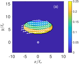
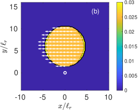
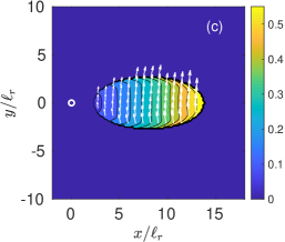
Figure 1: Velocity fields for off-axis rotating condensates with $\Omega=2\pi\times 2$Hz$\simeq 0.03\omega_{r}$. The colors illustrate the squared velocity field contours and the arrows represent the velocity field. In each panel the center of rotation is depicted with an open circle.

3.1.2 Hydrodynamical description in the rotating frame

The GP equation (4) can be written in a hydrodynamical form following a Madelung transformation $\psi=\sqrt{\rho}e^{i\theta}$, with $\rho(\mathbf{r},t)$ and $\theta(\mathbf{r},t)$ the density and phase profiles, respectively. In particular the continuity equation reads,

$$\frac{\partial\rho(\mathbf{r},t)}{\partial t}+\nabla.\left[\rho(\mathbf{V}(\mathbf{r},t)-\mathbf{\Omega}\times\mathbf{r})\right]=0\,,$$ (18)

where $\mathbf{V}(\mathbf{r},t)={\hbar}\nabla\theta/m$ is the superfluid velocity field in the laboratory frame. The stationary condition ${\partial\rho}/{\partial t}=0$ in the rotating frame thus implies $\nabla.[\rho(\mathbf{V}(\mathbf{r})-\mathbf{\Omega}\times\mathbf{r})]=0$. We first note that the trivial solution $\mathbf{V}(\mathbf{r})=\mathbf{\Omega}\times\mathbf{r}$ is not irrotational and therefore does not correspond to a superfluid. However, for an isotropic condensate in the $xy$-plane an homogeneous velocity field proportional to the center-of-mass position $\mathbf{r}_{\mathrm{cm}}$ of the form $\mathbf{V}(\mathbf{r})=\mathbf{\Omega}\times\mathbf{r}_{\mathrm{cm}}$ fulfills the above condition given that $\nabla\rho\perp[\mathbf{\Omega}\times(\mathbf{r}-\mathbf{r}_{\mathrm{cm}})]$ and $\nabla.[\mathbf{\Omega}\times(\mathbf{r}-\mathbf{r}_{\mathrm{cm}})]=0$ [56]. We note that such a solution is independent of the particular density profile, as it only requires that $\nabla\rho$ points in the $\mathbf{r^{\prime}}=\mathbf{r}-\mathbf{r}_{\mathrm{cm}}$ direction. When the circular symmetry is broken, it is natural to define $\mathbf{V}(\mathbf{r})=\mathbf{\Omega}\times\mathbf{r}_{\mathrm{cm}}+\delta\mathbf{v}(\mathbf{r})$, where $\delta\mathbf{v}(\mathbf{r})$ accounts for the deviation from the homogeneous value. For high filling numbers we can resort to the TF approximation to calculate the density profile in a displaced harmonic trap. Then, for small $\Omega$ we have

$$\rho\approx\rho_{\mathrm{TF}}=\frac{\mu}{g}-\frac{m}{2g}(\omega^{2}_{x}x^{\prime 2}+\omega^{2}_{y}y^{\prime 2}+\omega^{2}_{z}z^{\prime 2}),$$ (19)

and (18) reads

$$\nabla\rho(\mathbf{r})\,.\,\delta\mathbf{v}(\mathbf{r})+\rho(\mathbf{r})\,\nabla\cdot\delta\mathbf{v}(\mathbf{r})+\frac{m\Omega}{g}(\omega^{2}_{y}-\omega^{2}_{x})x^{\prime}y^{\prime}=0.$$ (20)

Since the superfluid is irrotational, $\nabla\times\mathbf{V}=0$, and this implies also that

$$\nabla\times\delta\mathbf{v}(\mathbf{r})=0.$$ (21)

Given that $\rho$ is a quadratic function of $\mathbf{r}^{\prime}$, the solution $\delta\mathbf{v}(\mathbf{r})$ of (20) and (21) must be linear on the coordinates in the TF approximation. Moreover, (21) implies that $\delta\mathbf{v}=(Ax^{\prime}+Cy^{\prime},Cx^{\prime}+By^{\prime},0)$. From (20) we finally obtain

$$\delta\mathbf{v}(\mathbf{r})=\Omega\epsilon_{0}(y^{\prime},x^{\prime},0),$$ (22)

where $\epsilon_{0}=\frac{\omega^{2}_{y}-\omega^{2}_{x}}{\omega^{2}_{y}+\omega^{2}_{x}}$ measures the anisotropy of the confinement. The order parameter can be written as

$$\psi(\mathbf{r})=|\psi(\mathbf{r})|\,e^{i\frac{m}{\hbar}\left[(\mathbf{r}-\mathbf{r}_{\mathrm{cm}})\cdot(\mathbf{\Omega}\times\mathbf{r}_{\mathrm{cm}})+\Omega\epsilon_{0}(x-x_{\mathrm{cm}})(y-y_{\mathrm{cm}})\right]},$$ (23)

where we have chosen the phase equal to zero at the position of the center of mass $\mathbf{r}_{\mathrm{cm}}$. In figure 2 we show the velocity field $\delta\mathbf{v}(\mathbf{r})$ extracted from GP simulations and illustrate how its contribution enhances the squared velocity field in different regions depending on the location of the rotation axis.

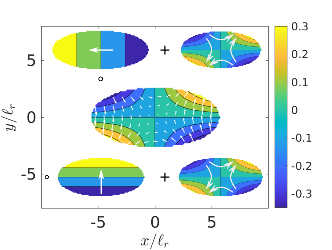
Figure 2: The central graph shows the velocity field $\delta\mathbf{v}(\mathbf{r})$ together with its phase extracted from the GP simulations for the case of the bottom panel of figure 1. The top and bottom insets show schemes of the decomposition of the total velocity field, $\mathbf{V}(\mathbf{r})=\mathbf{\Omega}\times\mathbf{r}_{\mathrm{cm}}+\delta\mathbf{v}(\mathbf{r})$, where the open circles mark the rotation axes. Such schemes represent the cases a) and c) of figure 1, respectively.

The anisotropy parameter $\epsilon_{0}$ also enters the angular momentum of the condensate per particle as

$$\langle L_{z}\rangle=m\Omega|\mathbf{r}_{\mathrm{cm}}|^{2}+m\Omega\epsilon_{0}[(\langle x^{2}\rangle-x^{2}_{\mathrm{cm}})-(\langle y^{2}\rangle-y^{2}_{\mathrm{cm}})],$$ (24)

which in turn shows that $\epsilon_{0}$ is proportional to the moment of inertia with respect to the center of mass $I^{\mathrm{cm}}=\langle L_{z}^{\mathrm{cm}}\rangle/\Omega=m\epsilon_{0}\left(\langle x^{\prime 2}\rangle-\langle y^{\prime 2}\rangle\right)$ in accordance with [57, 55]. The expression of $\epsilon_{0}$ as a function of the trapping frequencies corresponds to interacting atoms in the TF regime as shown previously by Recati et al. [55], whereas the analytic result of [57] corresponds to a gas with a Gaussian density profile.

When the condensate is circularly symmetric, $\epsilon_{0}=0$, the velocity field is homogeneous (see figure 1 (b)), and it should be equal to $\mathbf{v}_{\mathrm{cm}}={\boldsymbol{\Omega}}\times\mathbf{r}_{\mathrm{cm}}$. In such a case the order parameter takes the simpler form $\psi(\mathbf{r})=|\psi(\mathbf{r})|\,e^{i\frac{m}{\hbar}(\mathbf{r}-\mathbf{r}_{\mathrm{cm}})\,.\,(\mathbf{\Omega}\times\mathbf{r}_{\mathrm{cm}})}$. Similarly, for weakly linked condensates in rotating multiwell confining potentials, the WL function for site $k$ can be written as

$$w_{k}(\mathbf{r})=|w_{k}(\mathbf{r})|e^{i\frac{m}{\hbar}(\mathbf{r}-\mathbf{r}_{\mathrm{cm}}^{k})\cdot(\mathbf{\Omega}\times\mathbf{r}_{\mathrm{cm}}^{k})},$$ (25)

where $\mathbf{r}_{\mathrm{cm}}^{k}$ is the center of mass of the localized density $|w_{k}(\mathbf{r})|^{2}$.

3.2 Imprinted phases in rotating lattices

In this section we will first consider a four-site rotating lattice generated by the radial barriers on top of the toroidal trap as given by (17) and see how the linked condensates elongated in the $xy$ plane are transformed into almost circular ones by varying the values of $V_{b}$ and $\lambda_{b}$. This setup permits us to study the transition of the velocity fields from anisotropic condensates as that depicted in figure 1(a) to circularly symmetric ones as that shown in figure 1(b). Since for the condensates in this lattice one cannot obtain an analytic solution of the continuity equation (18), we shall directly solve the GP equation numerically for several lattice parameters.

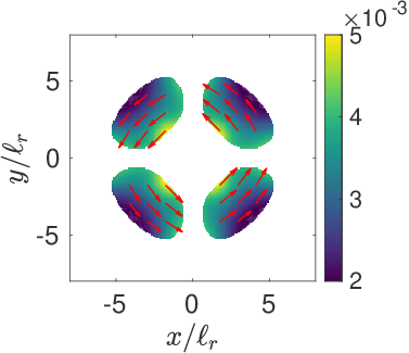
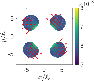
(a)	(b)
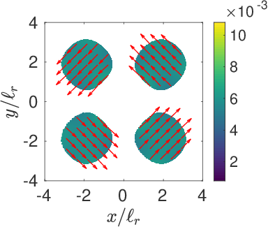
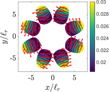
(c)	(d)

Figure 3: Velocity fields associated to each WL function for different rotating traps. The arrows correspond to the velocity field calculated with the GP equation and the colors mark the squared velocity field value in units of $\hbar^{2}/(m\ell_{r})^{2}$. In (a) and (b) the four-well toroidal trap with radial barriers (17) rotating at $\Omega/(2\pi)=1$Hz was considered in order to get inhomogeneous and homogeneous velocity fields, respectively fixing $\lambda_{b}/\ell_{r}=0.8$, $V_{b}/\hbar\omega_{r}=15$, and $\lambda_{b}/\ell_{r}=3$ and $V_{b}/\hbar\omega_{r}=21$, respectively. In (c) we employed the potential trap given by (16) and rotating at $\Omega/(2\pi)=2$Hz which yields an homogeneous velocity field. In (d) we considered eight wells in a lattice potential given by (17) rotating at $\Omega/(2\pi)=2$Hz with $\lambda_{b}/\ell_{r}=1.6$, and $V_{b}/\hbar\omega_{r}=20$, generating a velocity profile similar to that in figure 1 (c).

As we showed in section 3.1, the induced velocity field in an off-axis rotating harmonic condensate acquires a curvature that tilts in the direction of growth of the velocity field modulus, and this corresponds to a localized density profile that has no axial symmetry with respect to its center of mass. For a lattice in the tight-binding limit, one expects the same occurs to the induced velocity fields on the onsite localized WL functions, given that the effects of the junctions should be negligible. To observe such a behavior in ring-shaped optical lattices we numerically obtained the onsite localized WL function with the potentials introduced in section 2.2 rotating at different angular frequencies $\Omega$. In figure 3 we show the imprinted velocity fields, on each onsite localized function, for distinct trapping potentials: Panel (a) depicts the results for the lattice potential $V_{2}$, (17), with a narrow radial barrier $\lambda_{b}$ where the onsite localized density profiles extend in the angular direction and the velocity modulus increases when approaching the rotation axis, similar to figure 1(a). In panel (b) each onsite localized density profile is almost circularly symmetric with respect to its center of mass and the velocity field is homogeneous, while in figure 3(c) we can observe qualitatively the same profile but with a potential given by (16). Finally, in figure 3(d) we have considered the lattice potential with $N_{c}=8$. The parameters $V_{b}$ and $\lambda_{b}$ of (17) have been chosen in order to obtain onsite localized functions whose squared velocity field is similar to that shown figure 1(c). All these findings are in agreement with the results presented for single condensates subject to off-axis rotations in harmonic traps. Furthermore, the behavior of the velocity field curvature can be predicted from the analysis of the balance between the kinetic energy and the rotation energy terms as briefly discussed in the Appendix.

4 THE MULTIMODE PARAMETERS

4.1 Modulus of the parameters

In a rotating lattice the localized WL functions are modified respect to the nonrotating case due to the effective centrifugal force that opposes to the harmonic confinement. We thus expect all the model parameters to be affected: the onsite interaction parameter $U$ in our case is likely to increase, while the modulus of the hopping parameters $|J|$ and $|F|$ are expected to decrease as the density moves away from the center leading to a smaller overlap between neighboring WL functions. We have numerically investigated the model parameters for a condensate confined by the potential (16) as a function of $\Omega$. The rotation frequency has been varied keeping $\Omega<\omega_{r}$ to ensure the equilibrium of the condensate [55, 37]. In figure 4 we summarize the results.

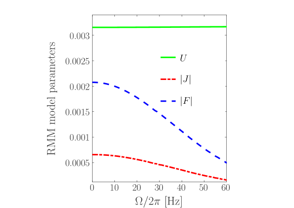
Figure 4: Absolute values of the RMM model parameters (in units of $\hbar\omega_{r}$) as functions of the rotation frequency $\Omega$ for the four-site potential well (16).

As it can be seen in the figure, the effect of the rotation on the onsite interaction parameter $U$ is negligible, while $|J|$ and $|F|$ strongly decrease as $\Omega$ gets larger. Therefore, the Peierls substitution $J\rightarrow|J|e^{i\Theta}$ ($F\rightarrow|F|e^{i\Theta}$) comprising only a change in the phase of the hopping parameters does not suffice as the modulus of $J$ and $F$ also depend on $\Omega$.

4.2 The phase of the hopping parameters

4.2.1 Relation between $\Theta$ and the velocity field circulation

The complex nature of the hopping parameters introduces the shift $\Theta$ given by (15). We will see that one can also determine $\Theta$ by using the order parameter of the MM model $\psi_{M}$ of (3) to calculate the velocity field circulation along a closed curve that passes through each junction.

Let $\mathcal{C}_{k}(\mathbf{r}_{k,k-1},\mathbf{r}_{k,k+1})$ be the circulation through the localized function $w_{k}$, from the junction $\mathbf{r}_{k,k-1}$ to the junction $\mathbf{r}_{k,k+1}$, and $\Delta\beta_{k}(\mathbf{r}_{k,k-1})$ be the jump of the phase in the junction between sites $k$ and $k-1$ produced by the imprinted velocity. The coordinates $\mathbf{r}_{k,k\pm 1}$ mark the positions of the junctions between the sites $k$ and $k\pm 1$. Using the time-dependent multimode model variables $\varphi_{k}(t)$, the circulation $\mathcal{C}_{k}$ must satisfy

$$\sum_{k}\mathcal{C}_{k}(\mathbf{r}_{k,k-1},\mathbf{r}_{k,k+1})\frac{m}{\hbar}+\sum_{k}\varphi_{k}(t)+\sum_{k}\Delta\beta_{k}(\mathbf{r}_{k,k-1})=2\pi\,l(t)$$ (26)

where $l(t)$ is related to the particular dynamics and is defined by $\sum_{k}\varphi_{k}(t)=2\pi\,l(t)$, where in this case we take $|\varphi_{k}(t)|<\pi$ to correctly define the direction of the associated time-dependent velocity field in the junctions. Then, we obtain

$$\sum_{k}\mathcal{C}_{k}(\mathbf{r}_{k,k-1},\mathbf{r}_{k,k+1})\frac{m}{\hbar}+\sum_{k}\Delta\beta_{k}(\mathbf{r}_{k,k-1})=0.$$ (27)

From the symmetry of the lattice, the jump in the phase is $\Delta\beta_{k}=\Delta\beta=\Theta$. If the velocity field in the localized WL function $w_{k}$ is homogeneous, and hence $\mathbf{V}^{k}(\mathbf{r})=\mathbf{\Omega}\times\mathbf{r}_{\mathrm{cm}}^{k}$, one can use (25) to calculate the circulation from $\mathbf{r}_{k,k-1}$ to $\mathbf{r}_{k,k+1}$ as their phase difference, yielding

$$\mathcal{C}^{H}_{k}=(\mathbf{r}_{k,k+1}-\mathbf{r}_{k,k-1})\cdot(\mathbf{\Omega}\times\mathbf{r}^{k}_{\mathrm{cm}}).$$ (28)

Taking into account the lattice symmetry, we have $|\mathbf{r}_{k,k+1}|=|\mathbf{r}_{k,k-1}|$ and $|\mathbf{r}^{k}_{\mathrm{cm}}|=|\mathbf{r}_{\mathrm{cm}}|,\forall k$. Additionally, from geometric considerations for circularly symmetric WL functions we can further simplify (28) to obtain

$$\mathcal{C}^{H}_{k}=\Omega|\mathbf{r}_{\mathrm{cm}}|^{2}\sin(2\pi/N_{c})$$ (29)

and hence, in terms of the average angular momentum

$$\Theta^{H}=-\frac{\langle L_{z}\rangle}{\hbar}\,\sin(2\pi/N_{c}).$$ (30)

In summary, for isotropic localized densities there exist a clear correspondence between the shift $\Theta$ and the angular momentum per particle given by (30). We numerically calculated $\langle L_{z}\rangle/\hbar$, and the phases $\theta_{J}$ and $\theta_{F}$ according to (9) and (12) for the potential trap (16) with $N_{c}=4$ by calculating the hopping parameters defined in (6) and (7), respectively. The results are shown in figure 5. The calculation confirms that there is a unique common shift $\Theta$ for the two hopping parameters and that its value follows the angular momentum as predicted by (30) when the velocity profile is homogeneous. Moreover, a slightly nonlinear dependence of $\Theta$ with $\Omega$ can be observed in figure  5 and can be attributed to the increase of $|\mathbf{r}_{\mathrm{cm}}|$ with rotation. We recall $\langle L_{z}\rangle$ given by (24) with $\epsilon_{0}=0$ yields $\langle L_{z}\rangle=m\Omega|\mathbf{r}_{\mathrm{cm}}|^{2}$.

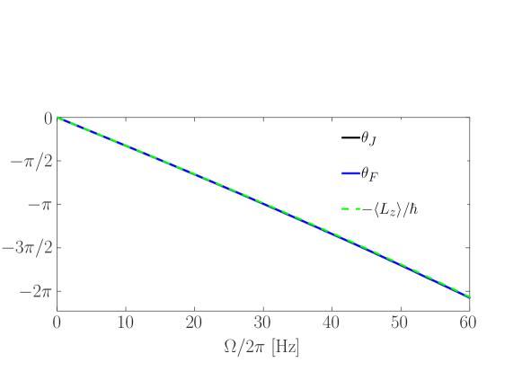
Figure 5: Phases $\theta_{J}$ and $\theta_{F}$ of the complex hopping parameters $J$ and $F$ respectively, and $-\langle L_{z}\rangle/\hbar$ as functions of the rotation frequency $\Omega$ for the confining potential of the form (16).

4.2.2 Relation between $\Theta$ and the Peierls phase

The rotation of a system at an angular frequency $\Omega$ gives rise to the effective vector potential $\mathbf{A}(\mathbf{r})=\mathbf{\Omega}\times\mathbf{r}$ whose circulation around a lattice plaquette determines the so-called Peierls phase [44]. Given that for $\mathbf{\Omega}=\Omega\hat{z}$, $\nabla\times\mathbf{A}(\mathbf{r})=2\Omega\hat{z}$ one can calculate such circulation around a given closed curve using the Stokes theorem as,

$$\oint\mathbf{A}(\mathbf{r}).d\mathbf{r}=N_{c}\,2\Omega\,S,$$ (31)

where $N_{c}S$ is the area enclosed by the curve. Contrary to the derivation using the vector potential, the calculation of the velocity field circulation (28) is independent of the curve and it only depends on the positions of the junctions. Moreover, we note that as our sites contain many particles the potential minima in general do not coincide with the centers of mass of the densities $\mathbf{r}_{\mathrm{cm}}^{k}$ defined by the WL functions in the $k$ sites. However, we show below that if one defines the closed polygon with vertices in each center of mass $\mathbf{r}_{\mathrm{cm}}^{k}$ and in the positions of the junctions $\mathbf{r}_{k,k+1}$ and $\mathbf{r}_{k,k-1}$, the Peierls phase and our result derived from the homogeneous velocity field coincide. Given that $(\mathbf{r}_{k,k+1}-\mathbf{r}_{k,k-1})\perp\mathbf{r}^{k}_{\mathrm{cm}}$, the points $\mathbf{r}_{k,k+1}$, $\mathbf{r}_{k,k-1}$, $\mathbf{r}^{k}_{\mathrm{cm}}$, and the origin of coordinates form a kite whose area is $S=|\mathbf{r}_{k,k+1}-\mathbf{r}_{k,k-1}||\mathbf{r}^{k}_{cm}|/2$. Hence, the circulation of the velocity field along the $k$ site given by (28) may be rewritten as

$$\mathcal{C}^{H}_{k}=(\mathbf{r}_{k,k+1}-\mathbf{r}_{k,k-1})\cdot(\mathbf{\Omega}\times\mathbf{r}^{k}_{\mathrm{cm}})=2\Omega S.$$ (32)

Such a result gives a total circulation $2\Omega SN_{c}$ in accordance with Peierls phases. The positions of the center of mass $\mathbf{r}_{\mathrm{cm}}^{k}$ and of the junctions $\mathbf{r}_{k,k+1}$ for each localized WL function are defined by

$$\mathbf{r}_{\mathrm{cm}}^{k} =\int\!\!d^{3}r\,w_{k}^{*}(\mathbf{r})\mathbf{r}\,w_{k}(\mathbf{r}),\quad\mathrm{and}$$ (33)

$$\mathbf{r}_{k,k+1} =\frac{1}{2}\int\!\!d^{2}r\,\left[w_{k}^{*}(\mathbf{r})+w_{k+1}^{*}(\mathbf{r})\right]\mathbf{r}\left[w_{k}(\mathbf{r})+w_{k+1}(\mathbf{r})\right],$$ (34)

respectively, where the last 2D integral is performed over the plane that contains $\mathbf{r}_{k,k+1}$ and it is defined by the angle $\vartheta=2\pi(k+1)/N_{c}$.

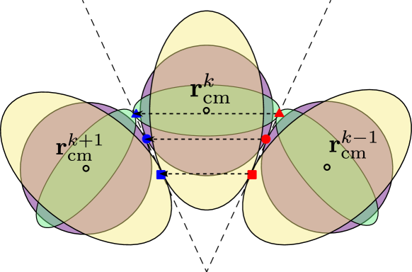
Figure 6: Schematic representation of the WL functions (ellipses), their junctions (solid symbols) and their center of mass (open circles) for ring-shaped multiwell condensates of different anisotropy. The dashed horizontal arrows mark the vectors $\mathbf{r}_{k,k+1}-\mathbf{r}_{k,k-1}$ joining the junctions of the $k$-site WL function. The solid circles, squares, and triangles correspond to circularly symmetric, prolate and oblate WL functions, respectively.

The simple correspondence between the angular momentum and $\Theta$ does not exist when the induced velocity field is inhomogeneous. Still, assuming a homogeneous velocity field, the circulation can be estimated by (28). As illustrated in figure 6, the anisotropy of the WL functions alters the position of the junctions yielding a lower circulation for a prolate WL function, and a higher circulation for an oblate one.

4.2.3 A numerical example

The breakdown of the correspondence shown in (30) between $\Theta$ and $\langle L_{z}\rangle$ as a consequence of the anisotropy of each localized density can be viewed in figure 7 for the configuration of figure 3 (d). The center of mass of the $k=0$ site is located at $\mathbf{r}_{\mathrm{cm}}^{0}=(4.9385,2.0456,0)\ell_{r}$, while the connecting junctions to the neighboring sites are $\mathbf{r}_{0,1}=(3.095,3.095,0)\ell_{r}$, and $\mathbf{r}_{0,-1}=(4.3776,0,0)\ell_{r}$. The phase difference $\mathcal{C}_{i}^{H}$ considering an homogeneous velocity field, thus, yields approximately $0.51$. However, from the intensity of the absolute value of the velocity field we may see from figure 3 (d), that it decreases from $\sqrt{0.024}\hbar/(m\ell_{r})$ to $\sqrt{0.02}\hbar/(m\ell_{r})$ and hence the actual velocity field circulation decreases to approximately $0.47$, which is in accordance with the value $\Theta=-0.474$ that we have obtained from its definition in (6). Such a correction is due to a nonvanishing eccentricity $\epsilon_{0}$ and hence cannot be taken into account by the circulation of the vector potential $\mathbf{A}$ only.

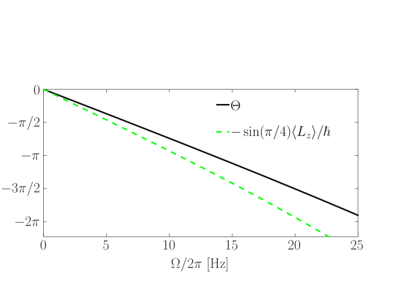
Figure 7: Hopping phase $\Theta=\theta_{J}=\theta_{F}$ and $-\sin(\pi/4)\langle L_{z}\rangle/\hbar$ (cf. (30)) as functions of the rotation frequency $\Omega$ for the lattice trap potential, (17), with $N_{c}=8$ sites, $N=10^{4}$ , $V_{b}/\hbar\omega_{r}=20$, and $\lambda_{b}/\ell_{r}=1.6$.

4.2.4 The velocity field near the junctions

The correct determination of the phase $\Theta$ within the RMM model permits an accurate description of the velocity field not only within the bulk of the onsite localized functions, but also around the junction. Indeed, in the RMM model the velocity field between neighbouring sites $k$ and $k+1$ can be obtained with great accuracy from the order parameter written as a combination of $w_{k}$ and $w_{k+1}$ only, as $\psi_{M}(\mathbf{r},t)\simeq\sqrt{n_{k}(t)}e^{i\phi_{k}(t)}w_{k}(\mathbf{r})+\sqrt{n_{k+1}(t)}e^{i\phi_{k+1}(t)}w_{k+1}(\mathbf{r})$. For the stationary state with $n=0$, this yields the velocity field

$$\mathbf{v}(\mathbf{r})=\frac{1}{N_{c}\rho}\biggr{\{}|w_{k}|^{2}\mathbf{V}^{k}(\mathbf{r})+|w_{k+1}|^{2}\mathbf{V}^{k+1}(\mathbf{r})+|w_{k}||w_{k+1}|\cos(\delta\alpha_{k})\left(\mathbf{V}^{k}(\mathbf{r})+\mathbf{V}^{k+1}(\mathbf{r})\right)\\ \left.+|w_{k}||w_{k+1}|\sin(\delta\alpha_{k})\frac{\hbar}{m}\left(\frac{\nabla|w_{k}|}{|w_{k}|}-\frac{\nabla|w_{k+1}|}{|w_{k+1}|}\right)\right\},$$ (35)

where, in the case of the four-site potential well (16), one has $\mathbf{V}^{k}(\mathbf{r})=\mathbf{\Omega}\times\mathbf{r}_{\mathrm{cm}}^{k}$, and $\delta\alpha_{k}=\dfrac{m}{\hbar}\mathbf{\Omega}\cdot[(\mathbf{r}_{\mathrm{cm}}^{k}-\mathbf{r}_{\mathrm{cm}}^{k+1})\times\mathbf{r}]$. The velocity field at the point $\mathbf{r}_{J}=(0,y_{\mathrm{CM}},0)$ with $y_{\mathrm{CM}}>0$ can be evaluated from (35) taking into account that $\delta\alpha_{k}=-\Theta$. In figure 8 we compare $\mathbf{v}_{J}=v_{J}\hat{x}$ obtained from the RMM model and the GP simulation as a function of $\Omega$. Given that $\Theta$ depends on the rotation frequency $\Omega$ as shown in figure 5, the magnitude and sign of $v_{J}$ is rather sensitive to the rotation. We may see that the RMM model correctly reproduces the peculiarities given by the GP equation. In fact, for $\Theta>-\pi$, that corresponds to frequencies $\Omega/2\pi\lesssim 28$ Hz, the velocity at the junction is positive, opposing to the $x$ component of the superposition of the velocity fields coming from the localized states on neighbouring sites, $\mathbf{V}^{k}(\mathbf{r})$. On the other hand, for $\Theta<-\pi$, the velocity at the junction reverses and points in the negative $\hat{x}$ direction.

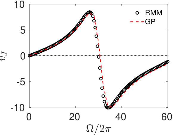
Figure 8: Velocity $\mathbf{v}_{J}=v_{J}\hat{x}$ at the junction $\mathbf{r}_{J}=(0,y_{\mathrm{CM}},0)$ as function of $\Omega$ for the potential trap given by (16). The circles correspond to the RMM model results and the dashed lines to the numerical GP solution. The trap parameters are the same as those in figure 3(c).

5 THE STATIONARY STATES

The energy levels $E_{n}$ can be written in terms of their stationary states $\psi_{n}$ as

$$E_{n}=\int d^{3}r\,\psi^{*}_{n}\Big{[}-\frac{\hbar}{2m}\nabla^{2}+V_{\mathrm{t}}-\Omega\hat{L}_{z}+\frac{gN}{2}|\psi_{n}|^{2}\Big{]}\psi_{n}$$ (36)

where the index $n$ refers to the winding number for $\Omega=0$. Due to the discrete $N_{c}$-fold rotational symmetry, the value of the circulation associated with the stationary state $\psi_{n}$ can be equal to the corresponding in a nonrotating case, that is to say $\hbar/m\,n$, or it can change in amounts of $\hbar/mN_{c}$. From figure 9 we numerically confirm this statement by evaluating the circulation around a centered box of side $\ell=2\ell_{r}$ as a function of $\Omega$ for the four stationary states with lower energy confined by the potential (16).

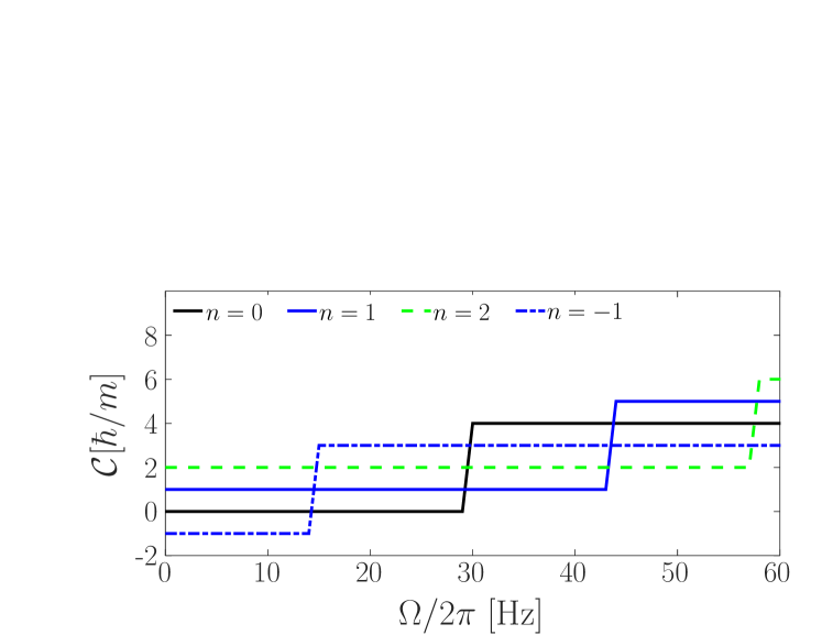
Figure 9: Velocity field circulation $\mathcal{C}$ (in units of $\hbar/m$) for the $n$ stationary state as a function of the rotation frequency $\Omega$ for the potential (16). The circulation is calculated along a centered square of side $\ell=2\ell_{r}$ in the $z=0$ plane.

In the RMM model the energy levels (36) are evaluated by inverting the basis transformation (1) and replacing $\psi_{n}$ into (36). Then, using the definitions for the RMM model parameters the energy levels take the simple form:

$$E_{n}=\epsilon+\frac{NU}{2N_{c}}-|K|\cos(\theta_{n}+\Theta),$$ (37)

where $\theta_{n}=2\pi n/N_{c}$, and $K=2J+\frac{4}{N_{c}}F$. It should be noted that when $4|F|/N_{c}>2|J|$, the phase of $K$, $\theta_{K}$ coincides with $\Theta$, as it happens in our case. Equation (37) provides a useful tool to test the accuracy of the RMM model. If the potential barriers are not high enough, or if the WL functions are not properly localized, the energies $E_{n}$ calculated from the GP equation will not satisfy (37). This can be used to select the trap parameters for the construction of a reliable model.

To characterize the energy levels structure it is useful to define the energy differences $\Delta E_{n}$ given by

$$\Delta E_{n} =E_{n}-E_{0}+|K|(1-\cos\Theta)$$

$$=|K|[1-\cos(\theta_{n}+\Theta)].$$ (38)

This description emphasizes the band structure of the energy levels in periodic systems [30, 29], but with $\theta_{n}$ shifted in $-\Theta$.

In figure 10 we illustrate the energy structure (38) for the case $N_{c}=8$. The curves correspond to the second line of the right hand side of (38) divided by $|K|$ and the symbols are obtained from the energy differences of the GP stationary states for each $\Omega$. The agreement between the curves and the symbols confirms the validity of the RMM model.

The states $\psi_{n}$ and $\psi_{-n}$, that are degenerate for $\Omega=0$, reach a maximum energy difference when $\Theta=-\pi/2$. For this rotation frequency, and assuming even $N_{c}$, the states $\psi_{N_{c}/2}$ and $\psi_{0}$ become degenerate.

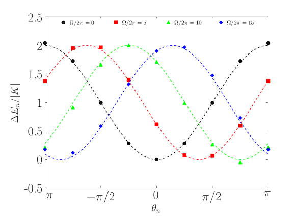
Figure 10: Band structure of the energy levels $E_{n}$ of the lattice trap potential $V_{2}$ with $N_{c}=8$ wells for the same parameters as in figure 7 and for rotation frequencies $\Omega/2\pi=0,5,10$, and $15$ Hz corresponding $\Theta/\pi=0,-0.37,-0.75$, and $-1.14$, respectively.

The energy ordering for each $n$ can be easily calculated for arbitrary $\Omega$ since the entire band moves by an amount $\Theta(\Omega)$ to the right assuming $\Omega>0$, which in turn is proportional to the angular momentum in the case of circularly symmetric onsite densities. Furthermore, the nonrotating ordering is restored when $\Theta=2\pi$, which corresponds to the rotation frequency

$$\Omega_{\mathrm{restore}}=\frac{2\pi\hbar}{mr_{\mathrm{cm}}^{2}\sin(2\pi/N_{c})}.$$ (39)

This rotation frequency $\Omega_{\mathrm{restore}}$ is further constrained to being below $\omega_{r}$ to ensure the confinement of the WL function.

6 SPECIAL MULTIMODE DYNAMICS VERSUS GROSS-PITAEVSKII SIMULATIONS

We have studied the accuracy of the RMM model comparing the solutions of (13) and (LABEL:ncmode2hn) with full 3D GP simulations for several initial conditions and rotation frequencies. In accordance with previous results for nonrotating traps [35, 26], we have found that to ensure a quantitative agreement between them one ought to take into account the onsite interaction energy dependence with the imbalance and hence employ the effective interaction parameter $U_{\mathrm{eff}}$ instead of the bare onsite $U$. It is worthwhile noticing that using the RMM model, the running time for the computation of the time evolution of populations and phase differences dramatically reduces by more than five orders of magnitude with respect to the that of a 3D numerical GP simulation.

Here we present some results for the four-well trap $V_{1}$ with $N=10^{4}$ and initial conditions given by $N_{1}=N_{-1}$, $N_{0}\neq N_{2}$ and $\varphi_{k}=0$. In this case we have found a value of $\alpha=0.219$ [26], irrespective of the rotation frequency. This choice of initial conditions allows us to analyze a particular effect of the rotation. If we set $\Omega=0$, the left-right reflection symmetry of the trapping potential ensures that $N_{1}(t)=N_{-1}(t)$ during the whole evolution. However, rotation breaks this symmetry in general. In the top (bottom) panel of figure 11 we show the population dynamics (phase differences) in each site corresponding to the GP simulations and the integration of the RMM model (13) and (LABEL:ncmode2hn). We focus on the particular choice of $\Omega/2\pi=15.065$Hz, which corresponds to a value of $\Theta$ close to $-\pi/2$ and hence the contributions to $|dn_{k}/dt|$ and $|d\varphi_{k}/dt|$ of the hopping terms are maximum at $t=0$. It is clear that in this case the initial symmetry is not maintained, and that the RMM model appropriately describes the dynamics.

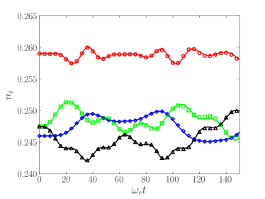
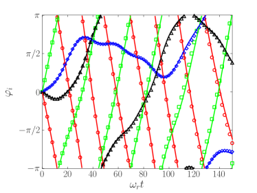
Figure 11: Population $n_{i}$ and phase differences $\varphi_{i}$ as functions of $t$ for $\Omega/2\pi=15.065$Hz. The solid lines and symbols correspond to results of the GP equation and RMM model, respectively. The initial conditions are given by $N_{-1}=2475$ (triangles), $N_{0}=2590$ (circles), $N_{1}=2475$ (squares), and $N_{2}=2460$ (diamonds) and $\varphi_{i}=0$. The reflection symmetry of the initial condition ($N_{-1}=N_{1}$) is clearly broken.

However, the structure of (13) and (LABEL:ncmode2hn) allows us to restore this symmetry if $\Theta=l\pi$, being $l$ a negative integer. The trap parameters employed in the dynamics with the potential given by (16) guarantees a homogeneous velocity field. Therefore, the associated rotation frequency $\Omega_{l}$ can be deduced from the mean value of the angular momentum $L_{z}=m\Omega\,r_{\mathrm{cm}}^{2}.$ For $l=-1$ a minus sign appears in the hopping parameters $J$ and $F$. The $\psi_{\pm n}$ states are degenerate again and the left-right reflection symmetry is recovered. The population dynamic for this case is shown in the top panel of figure 12, where we employed the same initial condition as in figure 11 but with a rotation frequency $\Omega=2\pi\times 30.13$Hz which gives a phase $\Theta\simeq-\pi$.

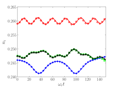
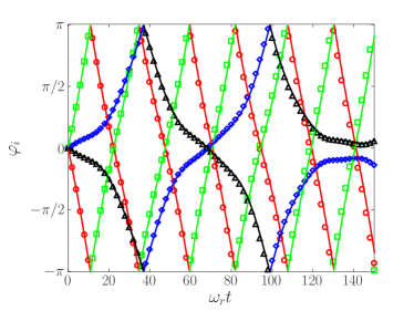
Figure 12: Population $n_{i}$ and phase differences $\varphi_{i}$ as functions of $t$ for $\Omega/2\pi=30.13$Hz for the same initial conditions as in figure 11. The solid lines and symbols correspond to results of the GP equation and RMM model, respectively. In this case $N_{1}=N_{-1}$ is maintained during the whole evolution.

Again, the RMM model predicts the same dynamics as the GP simulations. It is worthwhile to notice that such a restoration of the $N_{1}(t)=N_{-1}(t)$ symmetry is a pure quantum phenomenon, since the phase $\Theta$ is associated with the quantization of the velocity field circulation.

7 SUMMARY AND CONCLUDING REMARKS

We have formulated a rotating multimode model for a Bose-Einstein condensate confined in a ring-shaped optical lattice with $N_{c}$ sites. The appearance of induced inhomogeneous phases in the condensate implies that the onsite localized basis set cannot be taken as real functions, and hence the multimode hopping parameters $J$ and $F$ become complex numbers with the same phase $\Theta$. This was confirmed by numerically solving the Gross-Pitaevskii equations for several trap geometries.

To understand the nature of the induced velocity fields, as a first step we considered an off-axis rotating single condensate confined by an anisotropic harmonic trap. Varying the trapping frequencies in the orthogonal direction to the axis of rotation, we observed that the induced velocity field tilts in the direction of growth of the velocity modulus, and this corresponds to a density profile that has no axial symmetry with respect to its center of mass. When this axial symmetry is restored, the velocity field becomes homogeneous. On this last case, the complex phases of the localized basis can be easily predicted and a simple analytical relation between the hopping phase and the angular momentum is found by calculating the velocity field circulation. We have shown how these nontrivial imprinted phases can be analytically understood using the continuity equation for the density in the rotating frame.

In a second step, the induced velocity field was studied in rotating ring-shaped optical lattices for several geometries. It was found that for lattices in the tight-binding regime the velocity fields can be described in the same manner as in the single condensate case. For onsite homogeneous velocity fields, the phases of the hopping parameters are consistent with the Peierls phases appearing in systems subject to effective vector potentials. On the other hand, the effect of an inhomogeneity in the velocity field due to the lack of circular symmetry of the localized densities cannot be accounted for by the Peierls substitution formula alone. The full definition of the hopping parameters must be used to correctly calculate their phases. Finally, the validity of the rotating multimode model was verified for the first time by comparing its predictions with those obtained by numerically integrating the Gross-Pitaevskii equation for several initial conditions. In particular, we tested the rotating multimode model against nontrivial symmetry-preserved initial conditions and found they are accurately reproduced by the model. Finally, the RMM constitutes an extremely fast and accurate tool to predict the evolution of the population and phase differences, allowing to tackle also the dynamics of the velocity fields in multiple well systems. The model thus provides a promising tool to investigate features of the more complicated vortex dynamics. Work in this direction is in progress.

Appendix: Selection of the lattice parameters: balance of the energy contributions

In this Appendix we show how the confining potential of a ring-shaped lattice of the form (17) can be constructed in order to obtain an almost uniform velocity field in each site. This is analyzed by comparing the most important contributions to the energy for varying parameters of the confinement.

If one considers small barrier widths, one can assume that $\nabla\rho$ lies in the $\hat{r}$ direction far from the potential barriers, and hence the velocity field in the bulk can be approximated by $\mathbf{V}(\mathbf{r})=\dfrac{\mathcal{A}}{r}\hat{\theta}$, which verifies the continuity equation, $\nabla.[\rho(\mathbf{V}(\mathbf{r})-\mathbf{\Omega}\times\mathbf{r})]=0$. The amplitude $\mathcal{A}$ can be later chosen by enforcing a particular value of the angular momentum. On the other hand, in a general rotating optical lattice the velocity profile is determined by the competition between the increase of the kinetic energy due to the phase gradient in the bulk, and the reduction of the angular momentum term in the energy. We shall call such an energy balance $E_{r}$, which can be analyzed in the first quadrant thanks to the discrete symmetry of the lattice. Hence, writing the WL function at the first site ($k=0$) as $w_{0}(\mathbf{r})=|w_{0}(\mathbf{r})|e^{i\alpha_{0}(\mathbf{r})}$, this energy is given by

$$E_{r}\simeq\int d^{3}r\,w^{*}_{0}(\mathbf{r})\bigg{(}\frac{\hbar^{2}}{2m}|\nabla\alpha_{0}(\mathbf{r})|^{2}-\Omega\hat{L}_{z}\bigg{)}w_{0}(\mathbf{r}).$$ (40)

Although (40) cannot be analytically computed in general, an expression in terms of the mean values of the angular momentum per particle and of the spatial coordinates can be obtained in two special limits: a) when the onsite localized density is circularly symmetric, and b) when the barrier widths are small enough and thus $\nabla\rho$ lies in the radial direction. In a four-well trap ($N_{c}=4$), the WL function in the first site can be written as

$$w^{a}_{0}(\mathbf{r}) =|w^{a}_{0}(\mathbf{r})|e^{\textstyle i\frac{\langle\hat{L}_{z}\rangle}{\hbar}\frac{y-x}{\langle x\rangle+\langle y\rangle}}$$ (41)

for case a), and

$$w^{b}_{0}(\mathbf{r}) =|w^{b}_{0}(\mathbf{r})|e^{\textstyle i\frac{\langle\hat{L}_{z}\rangle}{\hbar}\theta}$$ (42)

for case b). Inserting (41) and (42) into (40) we obtain

$$E^{a}_{r}=\frac{1}{2m}\langle\hat{L}_{z}\rangle^{2}\frac{1}{\langle x\rangle^{2}+\langle y\rangle^{2}}-\Omega\langle\hat{L}_{z}\rangle$$ (43)

$$E^{b}_{r}=\frac{1}{2m}\langle\hat{L}_{z}\rangle^{2}\langle\frac{1}{x^{2}+y^{2}}\rangle-\Omega\langle\hat{L}_{z}\rangle$$ (44)

for case a) and b), respectively. Therefore, the sign of $\Delta E_{r}=E^{b}_{r}-E^{a}_{r}$ indicates the energetically favored velocity field for the system. For $\Delta E_{r}<0$, curved velocity fields are favored; whereas for large $\Delta E_{r}>0$ the velocity profiles are expected to be linear in each site and, in particular, consistent with (25). To confirm this connection between the minimization of $E_{r}$ and the velocity field curvature we numerically studied the velocity dispersion $\sigma_{v}^{2}=\langle\mathbf{v}^{2}\rangle-\langle\mathbf{v}\rangle^{2}$ in a given site for a set of values $(\lambda_{b},V_{b})$ corresponding to the potential $V_{2}$ (cf. (17)).

In figure 13 we present results for the dispersion $\sigma_{v}$ in the lattice potential $V_{2}$ with $N_{c}=4$. We show in colors the value of $\sigma_{v}$ in the $(\lambda_{b},V_{b})$ parameter space for $\Omega\simeq 0.014\omega_{r}$. The homogeneous velocity field region should lie to the right of the red solid curve marking where the minimum of the barrier equals the chemical potential in the absence of rotation, which is the condition for the condensates to be weakly linked. Below (above) the white curve, for which $\Delta E_{r}=0$, we have that $\Delta E_{r}<0$ ($\Delta E_{r}>0$). At the region where $\Delta E_{r}=0$, the velocity dispersion begin to decrease asymptotically to zero. This behavior confirms that the velocity field induced by the rotation of the lattice can be associated with the minimization of $E_{r}$.

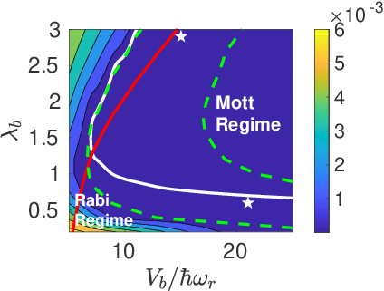
Figure 13: Velocity dispersion $\sigma_{v}$ (in arb. units) as a function of the lattice parameters $V_{b}$ and $\lambda_{b}$. The white solid curve marks $\Delta E_{r}=0$, while the red solid one marks the curve defined by $V_{b}=\mu(\Omega=0,\lambda_{b},V_{b})$. The region inside the dashed lines corresponds to the tight-binding regime bounded by Rabi (from below) and Mott-insulator (from above) regions. The white stars correspond to the values of $(\lambda_{b},V_{b})$ in the top panels of figure 3.

References

References

- [1] Jaksch D, Bruder C, Cirac J I, Gardiner C W and Zoller P 1998 Phys. Rev. Lett. 81 3108
- [2] Greiner M and Fölling S 2008 Nature 453 736
- [3] Bloch I, Dalibard J and Zwerger W 2008 Rev. Mod. Phys. 80 885
- [4] Morsch O and Oberthaler M 2006 Rev. Mod. Phys. 78 179
- [5] Henderson K, Ryu C, MacCormick C and Boshier M G 2009 New J. Phys. 11 043030
- [6] Lewenstein M, Sanpera A, Ahufinger V, Damski B, Sen A and Sen U 2007 Adv. Phys. 56 243–379
- [7] Dutta O, Gajda M, Hauke P, Lewenstein M, Lühmann D S, Malomed B A, Sowiński T and Zakrzewski 2015 Rep. Prog. Phys. 78 066001
- [8] Greiner M, Mandel O, Esslinger T, Hänsch T W and Bloch I 2002 Nature 415 39
- [9] Altman E, Polkovnikov A, Demler E, Halperin B I and Lukin M D 2005 Phys. Rev. Lett. 95 020402
- [10] Gross E P 1961 Nuovo Cimento 20 454; Pitaevskii L P 1961 Zh. Eksp. Teor. Fiz. 40 646 [Sov. Phys. JETP 13 451 ]
- [11] Smerzi A, Fantoni S, Giovanazzi S and Shenoy S R 1997 Phys. Rev. Lett. 79 4950
- [12] Raghavan S, Smerzi A, Fantoni S and Shenoy S R 1999 Phys. Rev. A 59 620
- [13] Ananikian D and Bergeman T 2006 Phys. Rev. A 73 013604
- [14] Melé-Messeguer M, Juliá-Díaz B, Guilleumas M, Polls A and Sanpera A 2011 New J. Phys. 13 033012
- [15] Abad M, Guilleumas M, Mayol R, Piazza F, Jezek D M and Smerzi A 2015 Europhys. Lett. 109 40005
- [16] Nigro M, Capuzzi P, Cataldo H M and Jezek D M 2017 Eur. Phys. J. D 71 297
- [17] Albiez M, Gati R, Fölling J, Hunsmann S, Cristiani M and Oberthaler M K 2005 Phys. Rev. Lett. 95 010402; Michael Albiez 2005 PhD Thesis (University of Heidelberg)
- [18] Ryu C, Andersen M, Cladé P, Vasant Natarajan, Helmerson K and Phillips W 2007 Phys. Rev. Lett. 99 260401
- [19] Ramanathan A, Wright K C, Muniz S R, Zelan M, Hill W T, Lobb C J, Helmerson K, Phillips W D and Campbell G K 2011 Phys. Rev. Lett. 106 130401
- [20] Wright K C, Blakestad R B, Lobb C J, Phillips W D and Campbell G K 2013 Phys. Rev. Lett. 110 025302
- [21] Eckel S, Lee J G, Jendrzejewski F, Murray N, Clark C W, Lobb C J, Phillips W D, Edwards M and Campbell G K 2014 Nature 506 200–203
- [22] Ryu C, Blackburn P W, Blinova A A and Boshier M G 2013 Phys. Rev. Lett. 111 205301
- [23] Aidelsburger M, Ville J L, Saint-Jalm R, Nascimbène S, Dalibard J and Beugnon J 2017 Phys. Rev. Lett. 119 190403
- [24] Cataldo H M and Jezek D M 2014 Phys. Rev. A 90 043610
- [25] Jezek D M and Cataldo H M 2013 Phys. Rev. A. 88 013636
- [26] Nigro M, Capuzzi P, Cataldo H M and Jezek D M 2018 Phys. Rev. A. 97 013626
- [27] Nigro M, Capuzzi P and Jezek D M 2018 Phys. Rev. A 98 063622
- [28] Pethick C J and Smith H 2008 Bose-Einstein Condensation in Dilute Gases (Cambridge: Cambridge University Press) chap. 14
- [29] Ferrando A 2005 Phys. Rev. E 72 036612
- [30] Pérez-García V M, García-March M A and Ferrando A 2007 Phys. Rev. A 75 033618
- [31] Cataldo H M and Jezek D M 2011 Phys. Rev. A. 84 013602
- [32] Jezek D M and Cataldo H M 2011 Phys. Rev. A. 83 013629
- [33] Ostrovskaya E A, Kivshar Y S, Lisak M, Hall B, Cattani F and Anderson D 2000 Phys. Rev. A 61 031601(R)
- [34] Ashcroft N W and Mermin N D 1976 Solid State Physics (Forth Worth: Saunders College Publishing) chap. 10
- [35] Jezek D M, Capuzzi P and Cataldo H M 2013 Phys. Rev. A 87 053625
- [36] Butts D A and Rokhsar D S 1999 Nature 397 327
- [37] Cooper N R 2008 Adv. Phys. 57 539
- [38] Fetter A L 2009 Rev. Mod. Phys. 81 647
- [39] Madison K W, Chevy F, Wohlleben W and Dalibard J 2000 Phys. Rev. Lett. 84 806–809
- [40] Abo-Shaeer J R, Raman C, Vogels J M and Ketterle W 2001 Science 292 476–-9
- [41] Bretin V, Stock S, Seurin Y and Dalibard J 2004 Phys. Rev. Lett. 92 050403
- [42] Williams R A, Al-Assam S and Foot C J 2010 Phys. Rev. Lett. 104 050404
- [43] Bhat R, Krämer M, Cooper J and Holland M J 2007 Phys. Rev. A 76 043601
- [44] Goldman N, Juzeliūnas G, Öhberg P and Spielman I B 2014 Rep. Prog. Phys. 77 126401
- [45] Jaksch D and Zoller P 2003 New J. Phys. 5 56
- [46] Dalibard J, Gerbier F, Juzeliūnas G and Öhberg P 2011 Rev. Mod. Phys. 83 1523–1543
- [47] Aidelsburger M, Nascimbene S and Goldman N 2018 Comptes Rendus Phys. 19 394–432
- [48] Jiménez-García K, LeBlanc L J, Williams R A, Beeler M C, Perry A R and Spielman I B 2012 Phys. Rev. Lett. 108 225303
- [49] Struck J, Ölschläger C, Weinberg M, Hauke P, Simonet J, Eckardt A, Lewenstein M, Sengstock K and Windpassinger P 2012 Phys. Rev. Lett. 108 225304
- [50] Aidelsburger M, Atala M, Lohse M, Barreiro J T, Paredes B and Bloch I 2013 Phys. Rev. Lett. 111 185301
- [51] Cole W S, Zhang S, Paramekanti A and Trivedi N 2012 Phys. Rev. Lett. 109 085302
- [52] Jin J, Han W and Zhang S 2018 Phys. Rev. A 98 063607
- [53] Peierls R 1933 Z. Phyzik 80 763
- [54] Pérez-García V M, García-March M A and Ferrando A, Phys. Rev. A 75, 033618 (2007).
- [55] Recati A, Zambelli F and Stringari S 2001 Phys. Rev. Lett. 86 377
- [56] In a rotating harmonic trap, due to the centrifugal force the center of mass, which coincides with the center of symmetry, is shifted to with respect to the center of the harmonic trap .
- [57] Stringari S 2017 Phys. Rev. Lett. 118 145302
- [58] Arwas G and Cohen D 2017 Phys. Rev. B 95 054505