Adaptive Traffic Control with Deep Reinforcement Learning: Towards State-of-the-art and Beyond

Abstract

In this work, we study adaptive data-guided traffic planning and control using Reinforcement Learning (RL). We shift from the plain use of classic methods towards state-of-the-art in deep RL community. We embed several recent techniques in our algorithm that improve the original Deep Q-Networks (DQN) for discrete control and discuss the traffic-related interpretations that follow. We propose a novel DQN-based algorithm for Traffic Control (called TC-DQN⁺) as a tool for fast and more reliable traffic decision-making. We introduce a new form of reward function which is further discussed using illustrative examples with comparisons to traditional traffic control methods.

1 Introduction

Transportation and urban mobility are the backbones of every major city’s infrastructure with direct impacts on health, environmental costs, and businesses. For instance, only in 2018 Americans lost 97 hours on average due to congestion, costing them nearly $87 billion—almost $1,348 per driver [1] and the demand is still steadily getting higher. As a consequence, there has been decades of attempts to integrate optimization and computational proficiency into traffic management and control [2]. Besides, with the advent of an unprecedented computing power, the research has lately observed remarkable increase in leveraging optimization and machine learning methods.

While early optimization tools for traffic signal control (e.g. SCOOT [3], SCATS [4]) are still employed in several large cities worldwide, they are non-adaptive in the sense that manual design for signal plans are required in practice. RL methods, on the other hand, possess an adaptive characteristic in sequential decision-making of traffic signals and have shown promising progress comparing to classic strategies in transportation. Nevertheless, the method is yet to be officially exercised in real scenarios due to fundamental shortcomings. For instance, training machine learning algorithms on real-world examples is dangerous, expensive, and time-consuming; thereby, RL models are mainly trained in simulations that often lack physical precision. Moreover, unlike domains with limited possible states (say, Atari games), adopting classic methods for highly complex environments such as transportation can be too ambitious.

In this work, we focus on such issues by (1) equipping our simulation environment with traffic scenarios that are created using real-world open-source data, and (2) incorporating the cutting-edge techniques in deep RL to improve our algorithm’s performance. In particular, inspired by the rainbow algorithm [5], we employ latest advancements on DQN including Double $Q$-Learning, Dueling Networks, and Prioritized Experience Replay (PER). We also take advantage of recent studies on novel exploration methods in RL as well as distributional forms of reward values and showcase the effectiveness of each technique on multiple traffic scenarios. Furthermore, we address a new form of discretized reward function as an additional requirement due to distributional RL technique (which is sensitive to rarely occurring events such as very smooth or highly congested traffic). Our empirical observations suggest that adding customized heuristics in the reward function can positively affect the performance. Finally, we provide illustrative case-studies wherein the benefits of our method as well as comparisons with some traditional architectures in Adaptive Traffic Signal Control (ATSC) are demonstrated on simulations that follow real traffic scenarios. Schematic of the idea behind our method is given in Figure 1.

The rest of the paper is organized as follows: Section 2 reviews the related literature. In Section 3, we provide some background. Section 4 defines the problem formulation followed by the experimental results in Section 5. Conclusions and future directions are addressed in Section 6.

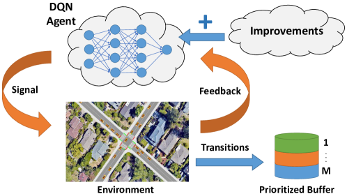
Figure 1: Schematic of our proposed algorithm.

2 RELATED WORK

Historically, traffic control has been one of the on-the-spot applications in science and engineering heavily due to the huge incurred expenses, health issues, and depleted natural resources that are caused from urban congestion and pollution. Moreover, research in traffic planning is highly restrictive in the sense that a newly proposed methodology should comprise: (1) computationally efficient implementation, and (2) minimal impractical assumptions. This line of work dates back to 1980’s with the advent of offline traffic light timing methods such as MAXBAND [6] where the scheme is selected through a self-regulatory process of multi-timing control which, in turn, was further improved using dynamic adjustment of parameters in methods such as SCOOT [3] and SCATS [4]. However, these products are suitable for regional traffic control and in many cases require considerable human intervention. Next generations of dynamic traffic control emerged in the following years (e.g. RHODES [7]) to address online control of time-varying traffic flows. This made the scheme more realistic but, meanwhile, highly expensive computationally. In general, the aforementioned methods face fundamental shortcomings including simplification of traffic constraints and lack of timely response to the actual traffic fluctuation [2, 8]

Fast forward a few decades, the so-called big data revolution has led to the integration of ideas from data-driven control and machine learning into transportation research. In particular, RL has been widely used to address traffic control due to its model-free nature [9, 10]. The results became even more promising after the breakthrough in deep RL, DQN [11]. Thereafter, the ATSC literature has been heavily focused on what type of RL algorithm to pick [12] and how to define RL parameters—i.e. states, rewards, and actions—to further enhance those algorithms [13]. Nevertheless, more recent advancements in RL are less tackled in traffic control literature. It is shown that the overall combination of these techniques results in a significantly improved performance on several instances of Atari games [5]. Similarly, we show that such combination plus heuristics in the RL problem definition leads to a substantially improved convergence on traffic control scenarios. A list of such methods includes—but is not limited to— Double Q-Learning [14], Prioritized Replay [15], Dueling Networks [16], NoisyNets [17], and distributional RL [18]. TC-DQN⁺ is an endeavour to show how such combinations contribute to the particular case of ATSC.

3 BACKGROUND

3.1 RL Notations and Background

An RL problem is defined as a Markov Decision Process (MDP) tuple $<\mathcal{S},\mathcal{A},\mathcal{T},r,\gamma>$ where the parameters respectively denote the set of states, set of possible actions, transition function, reward, and discount factor. At time-step $t$, the environment provides the agent with an observation (state) $s_{t}\in\mathcal{S}$, and the agent selects some action $a_{t}\in\mathcal{A}$. This interplay induces the transition $\mathcal{T}:\mathcal{S}\times\mathcal{A}\rightarrow\mathcal{S}$ defined as $\mathcal{T}(s,a,s^{\prime})=\mathbb{P}(s_{t+1}=s^{\prime}|s_{t}=s,a_{t}=a)$. As a consequence of taking the action, the environment provides the corresponding reward $r:\mathcal{S}\times\mathcal{A}\rightarrow\mathbb{R}$ defined at the state-action pair $(s,a)$ as $r_{t}(s,a)=\mathbb{E}[\mathcal{R}_{t}|s_{t}=s,a_{t}=a]$ and also the resulting state $s_{t+1}$ where $\mathcal{R}_{t}$ denotes the one-step reward. We assume an episodic MDP with constant $\gamma\in(0,1]$ and the goal of the agent is to maximize the expected return $G_{t}=\sum_{k=0}^{\infty}\gamma^{k}\mathcal{R}_{t+k}$ by finding an optimal policy $\pi^{*}$ through an iterative trial-and-error process. The RL agent learns the state-action value function ($Q$-function) $Q^{\pi}(s,a)=\mathbb{E}_{\pi}[G_{t}|s_{t}=s,a_{t}=a]$ following policy $\pi$ after action $a$ is taken at time $t$. The optimal value $Q^{*}(s,a)=\max_{\pi}Q^{\pi}(s,a)$ satisfies the Bellman optimality equation for $s\in\mathcal{S}$ and $a\in\mathcal{A}$,

$$Q^{*}(s,a)=\sum_{s^{\prime}\in\mathcal{S}}\mathcal{T}(s,a,s^{\prime})[r_{t}(s,a)+\gamma\max_{a^{\prime}}Q^{*}(s^{\prime},a^{\prime})].$$ (1)

3.2 Deep Q-Networks and Improvements

Unlike classic RL methods, DQN employs deep Neural Networks (NN) to approximate the $Q$-function in a nonlinear fashion, making RL applicable to high-dimensional problems [11]. In addition, the work uses two other pivotal techniques: using an experience replay buffer to remove data correlation and also integrating a less frequently updated target network to prevent fluctuations of $Q$-values in the Temporal Difference (TD) term of the loss defined as,

$$\mathcal{L}(\theta)=\mathbb{E}_{s,a,r,s^{\prime}\sim\mathcal{D}}\Big{[}\Big{(}\text{TD}_{\textit{target}}-Q(s,a;\theta)\Big{)}^{2}\Big{]},$$ (2)

where $\theta$ contains the parameters of the NN and $\text{TD}_{\textit{target}}=r_{t}(s,a)+\gamma\max_{a^{\prime}}Q(s^{\prime},a^{\prime};\theta^{-})$ where $\theta^{-}$ denotes periodic copies of $\theta$ and $\mathcal{D}$ is the (potentially time-varying) underlying distribution. Despite the initial success, the original DQN algorithm lacks stable and fast convergence in many cases due to poor exploration ($\epsilon$-greedy) and NN structure. There has been many independent attempts to improve the performance of DQN over the past few years. For instance, Double $Q$-Learning [14] addresses the overestimation bias in the maximization step in (1) resulting in the modified $\text{TD}_{\textit{target}}$,

$$\text{TD}_{\textit{target}}=r_{t}(s,a)+\gamma Q(s^{\prime},\text{argmax}_{a^{\prime}}Q(s^{\prime},a^{\prime};\theta);\theta^{-}).$$ (3)

Regarding the Experience Replay, PER [15] is an effort to assign higher priorities to those RL transitions with higher TD-error. New data are then inserted into a replay buffer with maximum priority, providing a bias towards more recent data. Another shortcoming of RL is that learning the expectation of returns, $G_{t}$, can be restrictive as the multimodality and the variance of similar actions (values) may not be preserved. This has been investigated over the years [19], and subsequently led to the idea of learning distributions—rather than expectation—of returns, referred to as distributional RL [18]. Lastly, there has been improvements due to NN architecture modifications. Namely, the Dueling Network structure [16] separates the learning streams of the value function and the advantage function. This lends more flexibility to learning in the sense that redundant actions become less influential when the value function prevails at some specific state. Furthermore, NoisyNets [17] modify the NN structure by adding noise to some hidden layers, whereas, unlike $\epsilon$-greedy, the parameters of the noise are adjusted by the model itself during training. This allows the agent to decide when and in what proportion to append uncertainty in NN parameters, making the exploration more efficient. In general, the methods introduced in this section have entailed promising improvement over the original DQN in accelerating the training and convergence. We will modify and utilize these techniques in ATSC.

4 PROBLEM FORMULATION

4.1 RL Environment and Agent

The RL environment is represented by a given intersection including vehicles with predefined probabilistic commutes (Figure 2). Containing the entire traffic regulation, the environment acts as a framework to provide feedback to the RL agent. We train our algorithm on Simulation of Urban MObility (SUMO)—an open-source and portable traffic simulator [20]. Traffic scenarios are generated in SUMO and adjusted from real-world data and observations (see Section 5). For brevity, in what follows the letters $N,E,S,$ and $W$ denote North, East, South, and West respectively, and $X\rightarrow Y$ implies from $X$ towards $Y$ ($X\leftrightarrow Y$ denotes both directions).

The RL agent is the decision-maker for the traffic light whose actions dictate the signal phase and cycle duration. In response, the agent receives a reward and the environment is shifted to the next iteration. The proper choice of RL states, actions, and rewards is crucial to any RL algorithm. We describe our selection as well as traffic-related interpretations of these parameters.

Actions. The set of actions, $\mathcal{A}$, includes available traffic signal patterns (Figure 3). The signal pattern is assumed to be non-sequential, i.e., the agent is free to choose any pattern (action) $a\in\mathcal{A}$ at each time-step. We set a minimum time, $T_{g}$, for each green light period to avoid sporadic flickers of the traffic light. The agent is free to stick to the current phase or move on to a fixed yellow phase, $T_{y}$, followed by an all-red interval, $T_{r}$, that are predefined to maintain smooth traffic. If the agent holds on to its current action, then $T_{y}=T_{r}=0$. Overall, the performance of our algorithm is highly sensitive to the integers $T_{g},T_{y},$ and $T_{r}$.

States. The state at time $t$, $s_{t}\in\mathcal{S}$, is a real vector that contains the information received from the environment. Often a number of measured elements (based on available sensing technology) are integrated to form the state vector (such as total wait time, queue length, etc. [21]).

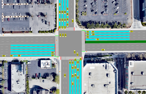
Figure 2: Snapshot of the RL environment. The blue strips show detectable range of sensors.

However, the usefulness of excessive application of various measures for the state is still questionable [22]. In our analysis, we set the state as the total number of vehicles within distance $d$ of the intersection on each lane (Figure 2) and collect those integers for $T_{g}$ consecutive frames after each action is taken. The aggregation of these frames and a one-hot key element—that determines the current phase—are concatenated to form $s_{t}\in\mathbb{N}_{\{0\}}^{n}$ where $n=|\mathcal{A}|T_{g}+1$ and $|\mathcal{A}|$ denotes the cardinality of $\mathcal{A}$. Note that such definition implicitly captures vehicles’ speeds without requiring to add extra dimensions, resulting in lower complexity and faster learning.

Rewards. Reward function, $r_{t}$, is a pivotal part of RL algorithm design as it is the feedback index to evaluate the quality of the agent’s performance. Common reward functions in traffic control are defined as a combination of elements such as queue length, wait time, throughput, etc., mostly accompanied with incidental factors (frequency of signal change, accident avoidance, etc.) [23, 24]. However, defining the reward function in this way is often not directly aimed at minimizing the total travel time of the vehicles at the intersection. Moreover, such rewards are highly sensitive to the weight of each factor, which makes the agent incapable of distinguishing between different learning measures [13].

We take a novel approach and define the reward function for state-action pair $(s,a)$ as,

$$r(s,a)=-\Big{(}r_{a}(s)+\mathbbm{1}_{\{t=T\}}r_{e}\Big{)}.$$ (4)

The action-based reward, $r_{a}$, captures the reward corresponding to action $a$ for $T_{g}$ frames and is defined as,

$$r_{a}(s)=\sum_{t=t_{a}}^{t_{a}+T_{g}}\Bigg{(}p_{1}\sum_{k=1}^{N_{a}}\omega_{t}^{k}(s)+p_{2}\mathbbm{1}_{\{N_{t}=0\}}\Bigg{)}+p_{3}\mathbbm{1}_{\{t_{a}\neq t_{a^{\prime}}\}},$$ (5)

where $\omega_{t}^{k}$ is a binary variable indicating whether vehicle $k$ is waiting at the intersection at time $t$, $t_{a}$ is the time-step at which action $a$ is employed, and $N_{a}$ is the total number of vehicles that pass through the intersection in the interval of $[t_{a},t_{a}+T_{g}]$. The term $\mathbbm{1}_{\{N_{t}=0\}}$ is considered to specify a penalty in case of a phase shift when there is no vehicle waiting—discouraging redundant actions. Further, the term $\mathbbm{1}_{\{t_{a}\neq t_{a^{\prime}}\}}$ indicates whether two consecutive signal phases are equal and is considered to oppose sporadic flickers of the traffic light. The variables $p_{1}$, $p_{2}$, and $p_{3}$ are the penalty weights. Overall, defining action-based rewards (as in Eq. (5)) is advantageous since it (1) enables the agent to have a measure of what actions lead to higher rewards, (2) naturally accounts for the temporal aspects of information such as ”speed of vehicles”, and (3) avoids unnecessary actions.

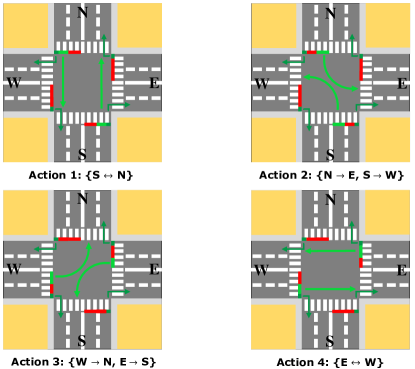
Figure 3: An example of the action set for a given intersection. Dark green implies yield to crossing lane.

The episodic reward, $r_{e}$, is a measure index to evaluate success or failure at the termination of each episode ($T$ indicates the length of an episode). However, in opposition to binary terminal rewards, we define,

$$r_{e}(\Omega_{T})=a\sigma\big{(}\eta(\Omega_{T}+\zeta)\big{)}+b,$$ (6)

where $\sigma(x)=1/(1+e^{-x})$ is the Sigmoid function, $\Omega_{T}=\sum_{k=1}^{N_{e}}\sum_{t=0}^{T}\omega_{t}^{k}$ is the total wait time of all vehicles in the corresponding episode, $N_{e}$ is the total wait time of all of the vehicles passing through the intersection during the episode $e$, and the parameters $a,\eta,\zeta,$ and $b$ depend on the particular traffic scenario. Unlike the action-based reward, the episodic reward captures the influence of “sequence of actions” throughout episode $e$. As demonstrated in Figure 4, the way we define $r_{e}$ results in a region of high rewards due to lower wait times (green) of the total number of vehicles throughout the episode. This is followed by a transition interval from high to low rewards (yellow). The steepness of this region can be adjusted with $\eta$. Finally, the transition induces a plateau region (red) where rewards worth similarly with respect to the wait time.

4.2 The Neural Networks Structure

We use a multilayered NN to estimate the $Q$-function. Figure 5 depicts a schematic of the NN structure in our proposed algorithm. The input layer of the network contains data from sensors and the output layer assigns values to actions in $\mathcal{A}$. As discussed in Section 4.1, the input and output layers contain $n=|\mathcal{A}|T_{g}+1$ and $|\mathcal{A}|$ neurons respectively. The input layer is followed by two hidden fully-connected layers with $n_{fc}$ neurons. The nonlinear approximation is exploited by Rectified Linear Unit (ReLU) for activation in our NN setup. Without the dashed box in Figure 5, original DQN algorithm is achieved. We further enhance the machinery using the tools we introduced in Section 3.2.

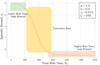
Figure 4: An example of the episodic reward function, $r_{e}$.

In summary, we split the network into value and advantage streams, each of which accommodating two hidden noisy layers with $n_{nl}$ neurons. The value (upper) stream results in one discrete probability distribution, where similar distributions are assigned to each action for the advantage (lower) stream. The output of these two streams are summed up to the final output layer. The output vector is then plugged into the loss function in (2) to update the weights of NN through backpropagation. As in DQN, at each optimization step, mini-batches of data are acquired from a prioritized replay buffer with a specified memory size. See Section 7 for notes on reproducing the algorithm.

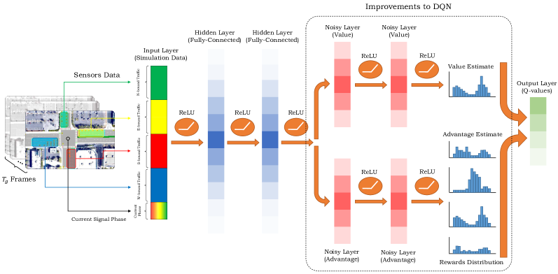
Figure 5: The structure of our proposed NN. The dashed box contains modifications to the DQN network.

5 EXPERIMENTS

5.1 Environment Design

In this section, we provide experiment results and compare them with baselines. We consider three environments that differ based on the number of actions and complexity of the state space. The environments are inspired by real intersections in San Francisco Bay Area (Figure 6). In-person observations integrated with real data (from [26]) are given to SUMO and the environmental hyperparameters are averaged over their real values. The result of the investigation is then reflected onto the vehicle generation rate as well as physical properties of the intersection such as minimum phase cycle ($T_{g}$, $T_{y}$, and $T_{r}$), number of lanes, right of way, etc., within the simulation environment. Meanwhile, to respect stochasticity of traffic flows we define,

$$X\sim\mathcal{B}(T,P_{e}),\hskip 11.38109pt\text{with}\hskip 11.38109ptP_{e}\sim\mathcal{U}(\ell,h),$$ (7)

where the random variable $X$ denotes the rate of traffic flow generated from a binomial distribution $\mathcal{B}$ with probability $P_{e}$ of vehicle generation per episode. We further assume that $P_{e}$ is a random variable uniformly sampled from the interval $[\ell,h]$ in order to enforce the entire range from low ($\ell$) to high ($h$) traffic flow randomly in the training stage. Our empirical results show that such randomness improves generalizability of our model to more traffic scenarios.

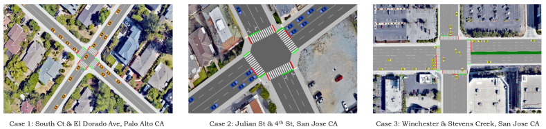
Figure 6: Case studies. The cases vary due to complexity of $\mathcal{S}$ and number of possible actions $|\mathcal{A}|$.

5.2 Results

The results of our experiments are threefold. First, we provide training trajectories to emphasize the improvement in the convergence of the algorithm. Second, we test our method on three different synthetic scenarios to show the generalizability of our algorithm when facing inconsistent traffic patterns. Finally, we provide ablation plots to qualitatively realize the contribution of each technique (from Section 3.2). We compare our results with the original (vanilla) DQN in addition to two other standard classic methods: (1) Fixed-Time (FT) [27] that utilizes a pre-specified phase cycle—mostly practiced for steady traffic—and (2) Self-Organizing Traffic Light (SOTL) [28] that functions when the number of waiting cars on a specific lane is above some hand-tuned threshold.

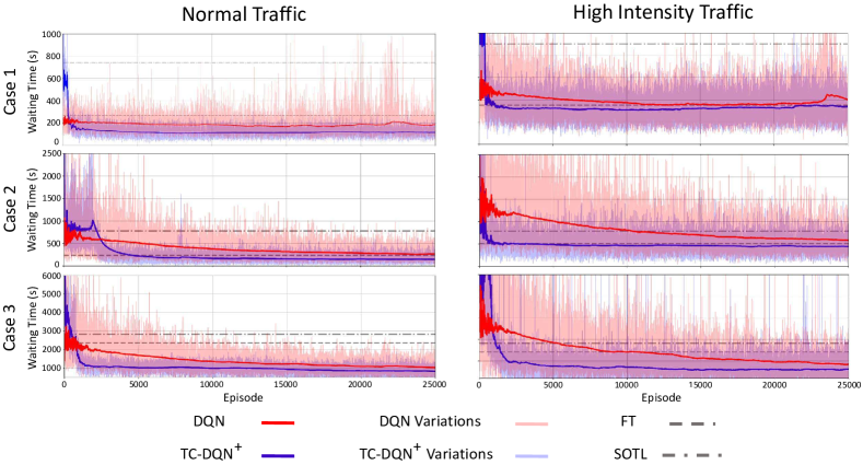
Figure 7: Total wait time learning trajectory of the vehicles at different intersections and traffic levels.

1) Convergence Results. We train our model on all three environments for two different traffic flows. First, we conduct training on the normal traffic patterns and then increase the flow to make the environment more complex and, hence, the learning more involved. Figure 9 depicts the total wait time of the vehicles based on the number of episodes the RL agent has been trained. The transparent red and blue lumps show the true total wait times of DQN and TC-DQN⁺ respectively at each episode and the bold curves denote the corresponding (decaying) weighted average. Moreover, the (average) wait time of FT and SOTL are also displayed for comparison. The monotonicity of the learning curves suggests the adaptive nature of RL algorithms in general (that methods such as FT and SOTL lack). However, the large gap between the behavior of TC-DQN⁺ and DQN trajectory—specifically, in the first 10,000 thousand episodes—verifies the effectiveness of the improvements to the DQN. Note the increase in the gap as the environment complexity and the traffic intensity get higher. In particular, Table 1 gives the time comparison between DQN and TC-DQN⁺. The entries display $\Delta\Omega_{T}$ for $T=400s$. For instance, at a relatively large intersection (case 3) and for normal traffic, an approximate of 200s total travel time is saved. For an average number of 30 vehicles commuting at this intersection for $T=400$ seconds, this becomes roughly 6s/vehicle of saved time.

Table 1: Time gap $\Delta\Omega_{T}=\Omega_{T}^{\text{TC-DQN}^{+}}-\Omega_{T}^{\text{\acs{DQN}}}$ (in seconds).

It is notable that while the standard measure of performance that we also consider is the “total wait time” of all vehicles ($\Omega_{T}$), the decrease in the variations (i.e. deviation of the true wait time from the weighted average) of RL algorithms shall not be neglected. These variations help to make sense of the robustness of the algorithm when facing unseen traffic scenarios. As Figure 9 suggests, variations of TC-DQN⁺ enjoy fast convergence whereas vanilla DQN shows regular unpredictable behavior in the long-term as the $\epsilon$-greedy exploration decays over time.

Table 2: Results on three environments (times in minutes). Lower wait time and higher reward imply better performance.

Figure 9 demonstrates the pertinence of wait time minimization to the exploration that leads to the convergence of actions and the rewards collection process in parallel (sampled for normal traffic scenario at case 3). The figure confirms the crucial role of efficient exploration (due to NoisyNets) and rewards collection (due to Distributional RL).

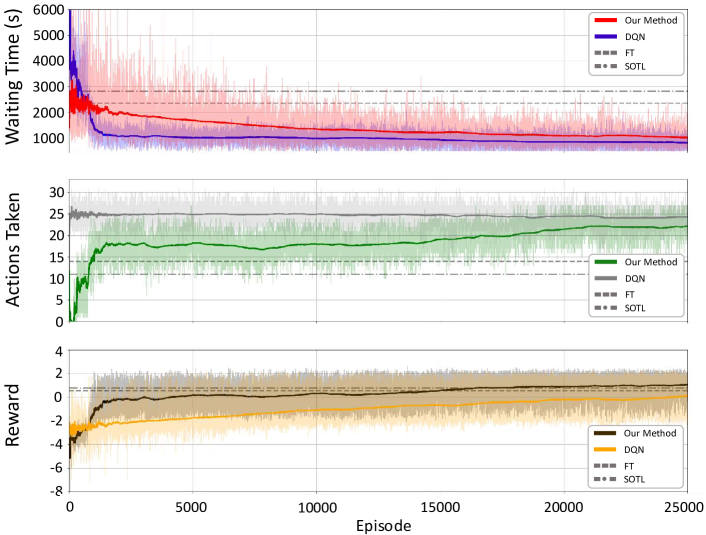
Figure 8: Training components in parallel.

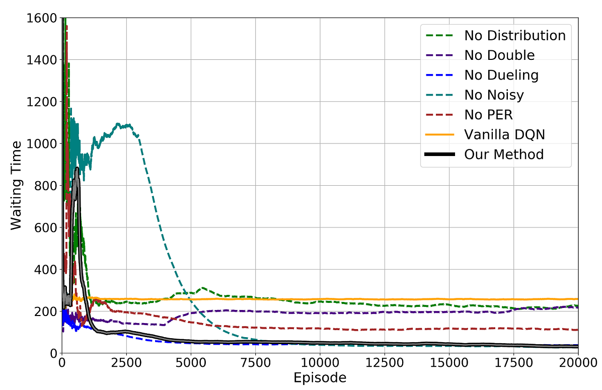
Figure 9: Ablation plots.

2) Test Cases. To test the performance of our model, we provide test cases on three synthetic scenarios defined as follows:

• Scenario I. Traffic on $E\leftrightarrow W$ is higher than $S\leftrightarrow N$.

• Scenario II. Traffic on $S\leftrightarrow N$ is higher than $E\leftrightarrow W$.

• Scenario III. Random equal traffic in all directions.

The results of the test cases are summarized in Table 2. As the table demonstrates, TC-DQN⁺ outperforms others in most of the traffic scenarios and environments. The results suggest that our algorithm performs best in traffic patterns wherein a pair of parallel directions (say, $S\leftrightarrow N$) are highly more crowded than the crossing routes ($E\leftrightarrow W$), and in some cases the improvement is substantial. For instance, for traffic scenario 1 at environment 3, $\Omega_{T}$ could be reduced by almost 2 hours in total comparing to the second best planner (FT) when the traffic is highly concentrated on $E\leftrightarrow W$. Also, TC-DQN⁺ surpasses DQN in every case, verifying the positive contributions of the techniques incorporated in the NN structure. Lastly, FT outperforms TC-DQN⁺ in two cases when the traffic flow is randomly generated in every direction (scenario 3). This is partly due to the form of reward function defined in Equation 4 as for complex environments, the $r_{a}$ and $r_{e}$ may not be clearly translated into an interpretable measure to the agent (for example, traffic scenario 3 of case 3). We foresee that refining the reward function with more theoretical grounding could resolve this shortcoming. This is addressed as a future direction.

3) Ablation Plots. As mentioned in Section 4.2, our methodology is a combination of several recent techniques from RL community. Accordingly, it is enlightening to realize the potential contribution of each of these methods to the final performance. The comparison is summarized in Figure 9 to showcase the median of total wait time among ablated variants (results are sampled for normal traffic at case 2). The most remarkable improvements are due to Distributional RL and Double Q-Learning where the absence of each technique results in a performance close to DQN. In addition, PER has a considerable role in upgrading the performance supporting effective use of data. Moreover, while NoisyNets is not contributing to the long-term performance or our algorithm, it enables convergence at fewer than 8000 episodes. Lastly, the portion of contributions of these techniques may vary according to the complexity of the environment. For instance, in the example that was provided in this section, Dueling Q-Learning does not contribute significantly as $|\mathcal{A}|$ is not large ($|\mathcal{A}|=2$). This could change for the case of environment 3 where $|\mathcal{A}|=4$ and the advantage stream of the NN is more discerned.

6 CONCLUSIONS

In this paper, we study a novel approach to integrate deep RL into traffic signal control at different urban intersections. We train our model, TC-DQN⁺, and test it on three different intersections ordered from simplest to most complex and generate traffic scenarios based on real data and on-site observations. Our results demonstrate significant improvement in the performance compared with the formerly employed methods using vanilla DQN.

We acknowledge that the current work is only one step towards faster and more reliable intelligent traffic control and can be improved in multitude of directions. One potential future route is to further examine the structure of the underlying NN to get more accurate nonlinear approximation of the traffic behavior. Moreover, there is room to combine our proposal with classic ATSC approaches for a better theoretical grounding of planning strategies. Last but not least, generalizability is crucial for data-driven traffic schemes. Hence, a potential next step is to make TC-DQN⁺ more robust to unpredictable phenomena such as roadblocks, constructions, accidents, etc.

7 Appendix: Reproducibility Guide

In this section, we provide necessary documentation to make the results of this work reproducible. We go over the required of hyperparameters and introduce the RL environments parameterization from Section 5. Note that the hyperparameters highly depend on the given problem. The values provided in this section regard test case 3 in our experiments. The psuedocode of TC-DQN⁺ algorithm is also provided to facilitate implementation.

RL Exploration. Whenever NoisyNets is off, we use $\epsilon$-greedy exploration as,

$$\epsilon_{t}=\epsilon_{f}+(\epsilon_{i}-\epsilon_{f})\exp({-t/\epsilon_{d}}),$$

where $\epsilon_{t}$ is the exploration factor at frame $t$, $\epsilon_{i}=1$ is the initial value, $\epsilon_{f}=0.05$ denotes the final exploration residual, and $\epsilon_{d}=15000$ is the decay factor. Otherwise, when using NoisyNets, we set $\epsilon_{t}=0$ and adjust $\sigma_{0}=0.4$ to initialize the weights of the noisy layers (see [17] for more details). The discount factor and episode length of the algorithm are set to $\gamma=0.99$ and $T=400s$ respectively.

NN Parameters. The NN takes data mini-batches of size $m=32$. The input, output, linear (fully-connected), and noisy layers each contains $n=41$, $|\mathcal{A}|=4$, $n_{fc}=512$, and $n_{nl}=64$ neurons respectively. The target network is updated with the frequency $t_{f}=10,000$ frames and we use Adam optimization [29] with learning rate $\xi=0.0002$.

PER. We consider a buffer memory size of $M=2^{20}$ samples. The priorities of transitions along with the importance sampling weights defined as,

$$p_{i}\propto\Big{|}\text{TD}_{\textit{target}}-Q(s,a;\theta)\Big{|}^{\omega_{i}},\hskip 25.60747pt\omega_{i}=\big{(}\frac{1}{M}\frac{1}{P(i)}\big{)}^{\beta},\hskip 25.60747ptP(i)=p_{i}^{\alpha}/\sum_{k}p_{k}^{\alpha},$$

where $P(i)$ is the probability of transition $i$, $\beta$ is the annealing factor initialized from $\beta_{0}=0.4$ and linearly increased to 1 with increments of $\Delta\beta=0.001$, and $\alpha=0.6$ adjusts the prioritization. The priorities are offset by $\varepsilon=0.01$ to prevent data from not being revisited when the TD-error is close to zero (see [15] for further details).

Distributional RL. Following the machinery in [18], we use discrete support $z$ to approximate the distribution of returns instead of the expected return defined by,

$$z^{i}=\nu_{\min}+(i-1)\frac{\nu_{\max}-\nu_{\min}}{N_{\text{dist}}-1},\hskip 22.76219pt\text{for}\hskip 5.69054pti\in\{1,\dots,N_{\textbf{dist}}\},$$

where $\nu_{\min}=-4$ and $\nu_{\max}=4$ are the minimum and maximum values of the distribution and $N_{\textbf{dist}}=41$ denotes the number of discrete bins (atoms).

Environment Settings. We set $T_{g}=10s$, $T_{y}=3s$, and $T_{r}=2s$ for the green, yellow, and all-red phase intervals respectively. For the episodic reward (defined in (6)), we set the parameters $a=3.5$, $b=-0.5$, $\eta=0.007$, and $\zeta=1000$. For the action-based reward, we let the weights $p_{1}=0.002$, $p_{2}=0.01$, and $p_{3}=0.1$. The vehicles’ speed limit is set equal to $v=40\ \text{km}/\text{h}$ and sensors range is set to $d=40m$.

Traffic Parameters. The three environment cases (see Figure 6) are different in the number of actions and complexity of the states (due to traffic level, lane changes, etc.). In particular, in case 1 (simplest case) left turns are not allowed (for instance $S\rightarrow W$, right turns are permitted in relevant lanes). In case 2, left turns are allowed but do not pose new actions (no separate light phase defined for left turns). Therefore, the crossing vehicles have to wait due to right of way of vehicles from the opposite direction. This is one of the main complexity factors in the test case scenarios with higher traffic intensity. Finally, Case 3 is the most complex environment where all types of signal phases are allowed.

Table 3 provides the parameters we used in the simulation to create these environments. The traffic level parameters are the probability of vehicle generation on corresponding lanes and due to different traffic levels as defined in SUMO. To find these probabilities, we use data from [26] and also conducted on-site in-person observations at intersections given in Figure 6 in San Francisco Bay Area. This was an effort to make the input to the simulations more realistic as RL trial-and-error is high-risk and impractical on real urban traffic.

Table 3: Traffic settings of our experiments.

Source Code Instructions. For the implementation of this work, we have used python 3.7.4, PyTorch 1.2 [30], OpenAI gym [31], and SUMO 1.3.1 [20]. The codes of our experiments are accessible on the GitHub repository of this project.

Algorithm 1 TC-DQN⁺ Algorithm

1:Initialize: Network with $\theta$ and target network with $\theta^{-}=\theta$

2:Input: replay buffer $\mathcal{D}$ with memory $M$, random variables $\varepsilon$ for the noisy networks, mini-batch size $m$, learning rate $\eta$, target update frequency $t_{f}$, discount factor $\gamma$, length of episodes $T$, hyperparameters for distributional RL $N_{\text{dist}}$, $\nu_{\min}$, $\nu_{\max}$, and hyperparameters for PER $\alpha$, $\beta$

3:For episode $e\in\{1,2,\dots\}$ do

4:       For $t=\{1,\dots,T\}$ do

5:            Initialize state $s_{0}\sim$ env

6:            Choose action $a_{t}\leftarrow\text{argmax}_{a^{\prime}\in\mathcal{A}}Q(s_{t},a^{\prime},\theta)$

7:            Run the environment and Sample $s_{t+1}$

8:            Obtain $r_{t}=r_{a_{t}}+r_{e}$ from (4), (5), and (6)

9:            Store transition $(s_{t},a_{t},r_{t},s_{t+1})$ in the buffer

10:            If $|\mathcal{D}|>M$ do

11:                 Delete oldest transition from $\mathcal{D}$

12:            Sample mini-batch of size $\min\{m,|\mathcal{D}|\}$ from $\mathcal{D}$

13:            Sample noisy variables for:     % Noisy networks initialization

14:                 the online network $\lambda\sim\varepsilon$

15:                 the target network $\bar{\lambda}\sim\varepsilon$

16:                 the action selection network $\bar{\bar{\lambda}}\sim\varepsilon$

17:            For $i\in\{1,\dots,m\}$ do     % Sampling from prioritized replay buffer

18:                 Sample transition $i\sim P(i)=p_{i}^{\alpha}/\sum_{j}p_{j}^{\alpha}$

19:                 Find PER weight $\omega_{i}=(MP(i))^{-\beta}/\max_{j}\omega_{j}$

20:                 Set $\text{TD}_{\text{target}}=r_{i}+\gamma\hat{Q}(s_{i},\text{argmax}_{a^{\prime}}Q(s_{i},a^{\prime},\theta,\lambda),\theta^{-},\bar{\lambda})$

21:                 Find TD-error $\delta_{i}=\text{TD}_{\text{target}}-Q(s_{i-1},a_{i-1},\theta,\lambda)$

22:                 Update transition priority $p_{i}\leftarrow|\delta_{i}|$

23:                 If $s_{t+1}$ is a terminal state do

24:                        $\hat{Q}\leftarrow r_{i}$

25:                 Else do

26:                        $\hat{Q}(s_{i},b^{\prime},\theta^{-},\bar{\lambda})\leftarrow\sum_{j}z_{j}p_{j}(s_{i},b^{\prime})$

27:                        $b\leftarrow\text{argmax}_{b^{\prime}\in\mathcal{A}}\hat{Q}(s_{i},b^{\prime},\theta^{-},\bar{\bar{\lambda}})$     % action with double Q-learning

28:                        $m_{j}\leftarrow 0$ for $j=\{0,\dots,N_{\text{dist}}-1\}$

29:                        For $k=\{1,\dots,N_{\text{dist}}\}$ do     % Discrete distribution of returns

30:                             $Tz_{k}\leftarrow[r_{t}+\gamma z_{k}]_{\nu_{\min}}^{\nu_{\max}}$

31:                             $c_{k}\leftarrow(Tz_{k}-\nu_{\min})/\Delta z$

32:                             $l\leftarrow\left\lfloor c_{k}\right\rfloor,\ u\leftarrow\left\lceil c_{k}\right\rceil$

33:                             $m_{l}\leftarrow m_{l}+p_{k}(s_{t+1},b_{t})(u-c_{k})$

34:                             $m_{u}\leftarrow m_{u}+p_{k}(s_{t+1},b_{t})(c_{k}-l)$

35:                        Set Loss $\mathcal{L}=-\sum_{j}m_{j}\omega_{i}\log p_{j}(s_{t},a_{t})$

36:                        Do a gradient step with $\theta\leftarrow\theta-\eta\nabla\mathcal{L}$

37:       If $e\times t\equiv 0$ (mod $t_{f}$) do

38:            Update the target network $\theta^{-}\leftarrow\theta$

References

- [1] “INRIX global traffic scorecard.” https://inrix.com/scorecard/.
- [2] H. Wei, G. Zheng, V. Gayah, and Z. Li, “A survey on traffic signal control methods,” arXiv preprint arXiv:1904.08117, 2019.
- [3] P. Hunt, D. Robertson, R. Bretherton, and R. Winton, “SCOOT-a traffic responsive method of coordinating signals,” tech. rep., 1981.
- [4] P. Lowrie, “SCATS, Sydney coordinated adaptive traffic system: A traffic responsive method of controlling urban traffic,” 1990.
- [5] M. Hessel, J. Modayil, H. Van Hasselt, T. Schaul, G. Ostrovski, W. Dabney, D. Horgan, B. Piot, M. Azar, and D. Silver, “Rainbow: Combining improvements in deep reinforcement learning,” in Thirty-Second AAAI Conference on Artificial Intelligence, 2018.
- [6] J. D. Little, M. D. Kelson, and N. H. Gartner, “MAXBAND: A versatile program for setting signals on arteries and triangular networks,” Transportation Research Record, no. 795, 1981.
- [7] P. Mirchandani and L. Head, “A real-time traffic signal control system: architecture, algorithms, and analysis,” Transportation Research Part C: Emerging Technologies, vol. 9, no. 6, pp. 415–432, 2001.
- [8] Y. Wang, X. Yang, H. Liang, and Y. Liu, “A review of the self-adaptive traffic signal control system based on future traffic environment,” Journal of Advanced Transportation, 2018.
- [9] S. Mikami and Y. Kakazu, “Genetic reinforcement learning for cooperative traffic signal control,” in Proceedings of the First IEEE Conference on Evolutionary Computation, pp. 223–228, 1994.
- [10] L. Prashanth and S. Bhatnagar, “Reinforcement learning with function approximation for traffic signal control,” IEEE Transactions on Intelligent Transportation Systems, vol. 12, no. 2, pp. 412–421, 2010.
- [11] V. Mnih et al., “Human-level control through deep reinforcement learning,” Nature, vol. 518, no. 7540, p. 529, 2015.
- [12] W. Genders and S. Razavi, “An open-source framework for adaptive traffic signal control,” arXiv preprint arXiv:1909.00395, 2019.
- [13] H. Wei, G. Zheng, H. Yao, and Z. Li, “Intellilight: A reinforcement learning approach for intelligent traffic light control,” in Proceedings of the 24th ACM SIGKDD International Conference on Knowledge Discovery & Data Mining, pp. 2496–2505, ACM, 2018.
- [14] H. Van Hasselt, A. Guez, and D. Silver, “Deep reinforcement learning with double -learning,” in Thirtieth AAAI conference on artificial intelligence, 2016.
- [15] T. Schaul, J. Quan, I. Antonoglou, and D. Silver, “Prioritized experience replay,” CoRR, vol. abs/1511.05952, 2016.
- [16] Z. Wang, T. Schaul, M. Hessel, H. Hasselt, M. Lanctot, and N. Freitas, “Dueling network architectures for deep reinforcement learning,” in International conference on machine learning, pp. 1995–2003, 2016.
- [17] M. Fortunato et al., “Noisy networks for exploration,” in International Conference on Learning Representations, 2018.
- [18] M. G. Bellemare, W. Dabney, and R. Munos, “A distributional perspective on reinforcement learning,” in Proceedings of the 34th International Conference on Machine Learning-Volume 70, pp. 449–458, 2017.
- [19] T. Morimura, M. Sugiyama, H. Kashima, H. Hachiya, and T. Tanaka, “Parametric return density estimation for reinforcement learning,” in Proceedings of the Twenty-Sixth Conference on Uncertainty in Artificial Intelligence, pp. 368–375, 2010.
- [20] D. Krajzewicz, G. Hertkorn, C. Rössel, and P. Wagner, “SUMO (Simulation of Urban MObility)-an open-source traffic simulation,” in Proceedings of the 4th middle East Symposium on Simulation and Modelling, pp. 183–187, 2002.
- [21] M. Aslani, M. S. Mesgari, and M. Wiering, “Adaptive traffic signal control with actor-critic methods in a real-world traffic network with different traffic disruption events,” Transportation Research Part C: Emerging Technologies, vol. 85, pp. 732–752, 2017.
- [22] G. Zheng, X. Zang, N. Xu, H. Wei, Z. Yu, V. Gayah, K. Xu, and Z. Li, “Diagnosing reinforcement learning for traffic signal control,” arXiv preprint arXiv:1905.04716, 2019.
- [23] T. Nishi, K. Otaki, K. Hayakawa, and T. Yoshimura, “Traffic signal control based on reinforcement learning with graph convolutional neural nets,” in 21st IEEE International Conference on Intelligent Transportation Systems (ITSC), pp. 877–883, 2018.
- [24] I. Arel, C. Liu, T. Urbanik, and A. G. Kohls, “Reinforcement learning-based multi-agent system for network traffic signal control,” IET Intelligent Transport Systems, vol. 4, no. 2, pp. 128–135, 2010.
- [25] R. S. Sutton and A. G. Barto, Reinforcement learning: An introduction. MIT press, 2018.
- [26] “Open Data San Francisco.” https://datasf.org/.
- [27] A. J. Miller, “Settings for fixed-cycle traffic signals,” Journal of the Operational Research Society, vol. 14, no. 4, pp. 373–386, 1963.
- [28] S.-B. Cools, C. Gershenson, and B. D’Hooghe, “Self-organizing traffic lights: A realistic simulation,” in Advances in applied self-organizing systems, pp. 45–55, Springer, 2013.
- [29] D. P. Kingma and J. Ba, “Adam: A method for stochastic optimization,” arXiv preprint arXiv:1412.6980, 2014.
- [30] A. Paszke et al., “Pytorch: An imperative style, high-performance deep learning library,” in Advances in Neural Information Processing Systems 32, pp. 8024–8035, 2019.
- [31] G. Brockman, V. Cheung, L. Pettersson, J. Schneider, J. Schulman, J. Tang, and W. Zaremba, “OpenAI Gym,” arXiv preprint arXiv:1606.01540, 2016.