On Asymptotic Dynamical Regimes of Manakov -soliton Trains in Adiabatic Approximation
Abstract
We analyze the dynamical behavior of the -soliton train in the adiabatic approximation of the Manakov model. The evolution of Manakov -soliton trains is described by the complex Toda chain (CTC) which is a completely integrable dynamical model. Calculating the eigenvalues of its Lax matrix allows us to determine the asymptotic velocity of each soliton. So we describe sets of soliton parameters that ensure one of the two main types of asymptotic regimes: the bound state regime (BSR) and the free asymptotic regime (FAR). In particular we find explicit description of special symmetric configurations of solitons that ensure BSR and FAR. We find excellent matches between the trajectories of the solitons predicted by CTC with the ones calculated numerically from the Manakov system for wide classes of soliton parameters. This confirms the validity of our model.
Keywords: Manakov model, soliton interactions, adiabatic approximations complex Toda chain
1 Introduction
The solitons and their interactions find numerous applications of in many areas of today nonlinear physics, such as hydrodynamics, nonlinear optics, Bose-Einstein condensates, etc. [28, 2, 27, 3, 34, 1, 7]. This explains why it is important to study their interactions. The first results on soliton interactions were obtained by Zakharov and Shabat [36, 35]. There they proved that the nonlinear Schrödinger equation
| (1) |
can be integrated by the inverse scattering method (ISM). Then they constructed the -soliton solution of (1) and calculated their limits for and , assuming that all solitons have different velocities. Comparing the asymptotics they concluded that the soliton interactions are purely elastic, i.e., no new solitons can be created. In addition the solitons preserve their amplitudes and velocities, and the only effect of the interactions are relative shifts of the center of masses and phases.
Later Karpman and Solov’ev proposed another approach to the soliton interactions based on the adiabatic approximation [26, 25]. They proposed to model the -soliton trains of the NLS eq. (1). By -soliton train they meant a solution of the NLS eq. with initial condition:
| (2) | ||||||
The adiabatic approximation holds true if the soliton parameters satisfy [26]:
| (3) |
where , and are the average amplitude and velocity respectively. In fact we have two different scales:
In this approximation the dynamics of the -soliton train is described by a dynamical system for the soliton parameters. What Karpman and Solov’ev did was to derive the dynamical system for the two soliton interactions: a system of 8 equations for the 8 soliton parameters. They were able also to solve it analytically.
Later their results were generalized to -soliton trains [17, 24, 16]. The corresponding model can be written down in the form :
| (4) | ||||
where and
| (5) | ||||
Obviously the system (4) becomes the Toda chain with free ends for the complex variables :
| (6) |
which is known as the complex Toda chain (CTC).
It is well known that the standard (real) Toda chain is an integrable system [31, 28, 9]. In the case of (6), which is known as Toda chain with open ends, it was possible to write down its solutions explicitly [31]. An important fact is that these solutions depend analytically on their parameters and can be easily generalized to the CTC.
In fact some time ago a special configurations of soliton trains that are modeled by the real Toda chain [4, 5]. To this end we must choose solitons with equal amplitudes (i.e., ), vanishing initial velocities (, and out-of phase . It is easy to see that under these assumptions become real valued and (6) become the standard Toda chain.
The adiabatic approach of Karpman and Solov’ev has a drawback: it is an approximate method whose precision is determined by . On the other hand it has the advantages: first, it is not limited only to solitons with different velocities, and second, it can take into account possible perturbations of the NLS [17, 24, 16].
Another important generalization of the NLS equation is known as the Manakov model [28] (vector NLS):
| (7) |
The corresponding vector -soliton train is determined by the initial condition:
| (8) | ||||||
where the constant polarization vector is normalized by
Therefore each Manakov soliton is parametrized by 6 parameters.
It was natural to extend the Karpman-Solov’ev method to the Manakov model. The result is known as the generalized CTC (GCTC) [10, 11, 14, 12]. Of course later the GCTC was also adapted to treat the effects of several types of perturbations on solitons [13, 33, 19, 30, 32, 8].
The advantage of the integrability of the CTC and GCTC is in the fact that knowing the initial set of soliton parameters one can predict the asymptotic regime of the soliton train [17, 24, 16]. On the other hand it is possible to find the set of constraints on the soliton parameters that would ensure given asymptotic regime. These constraints were derived and analyzed for and -soliton trains; for larger number of solitons only fragmentary results such as the quasi-equidistant propagation of solitons [16].
The aim of the present paper is to reinvestigate these results and to demonstrate several configuration of multisoliton trains for which one can predict that they will go into bound state regime (BSR) or into free asymptotic regime (FAR). In Section 2 we outline the derivation of the GCTC model, see eq. (16) below which now depends also on the polarization vectors and models the behavior of the -soliton train of the vector NLS. We also formulate the Lax representation for the GCTC and explain how it can be used to determine the asymptotic regime of the soliton train. In Section 3 we formulate two classes of explicit constraints on the soliton parameters that are responsible for BSR and FAR. The first class are generic conditions that ensure that the Lax matrix becomes either real or purely imaginary. The second class are based on special explicit constraints on the soliton parameters that make the eigenvalues of the Lax matrix proportional to each and easier to establish if they are real ir purely imaginary.
2 Preliminaries
2.1 Variational Approach and Generalized CTC
The Lagrangian of the vector NLS perturbed by external potential is:
| (9) |
Then the Lagrange equations of motion:
| (10) |
coincide with the vector NLS with external potential .
Next we insert (see eq. (8)) and integrate over neglecting all terms of order and higher. In doing this we assume that at and use the fact, that only the nearest neighbor solitons will contribute. All integrals of the form:
| (11) |
with can be neglected. The same holds true also for the integrals
where at least three of the indices have different values. In doing this key role play the following integrals:
| (12) | ||||
Thus after long calculations we obtain:
| (13) | ||||||
where
| (14) |
The equations of motion are given by:
| (15) |
where stands for one of the soliton parameters: , , , and . The corresponding system is a generalization of CTC:
| (16) | ||||
where again and the other variables are given by (5). Now we have additional equations describing the evolution of the polarization vectors. But note, that their evolution is slow, and in addition the products multiply the exponents which are also of the order of . Since we are keeping only terms of the order of we can replace by their initial values
| (17) |
We will consider most general form of the polarization vectors:
| (18) |
In our previous papers we considered configurations for which are real, i.e., . Note that the effect of the polarization vectors could be viewed as change of the distance between the solitons and between the phases.
The system (16) was derived for the Manakov system by other methods in [18]. There the GCTC model it was tested numerically and found to give very good agreement with the numerical solution of the Manakov model. However the tests were done only for real values of the polarization vectors, i.e., all , . Below we will take into account the effect of onto the dynamical regimes of the solitons.
2.2 Asymptotic Regimes: General Approach
We first briefly remind the main results concerning the CTC model [17, 24, 16, 14, 18]. The CTC is completely integrable model; it allows Lax representation , where:
| (19) |
where , and the matrices are determined by . The eigenvalues of are integrals of motion and determine the asymptotic velocities.
The GCTC derived in [10, 11, 14, 18, 12] is also a completely integrable model. It allows Lax representation just like the standard real Toda chain [9, 31, 29] , where:
| (20) |
where , . Like for the scalar case, the eigenvalues of are integrals of motion. If we denote by (resp. ) the set of eigenvalues of (resp. ) then their real parts (resp. ) determine the asymptotic velocities for the soliton train described by CTC (resp. GCTC). Thus, starting from the set of initial soliton parameters we can calculate (resp. ), evaluate the real parts of their eigenvalues and thus determine the asymptotic regime of the soliton train.
- Regime (i)
- Regime (ii)
-
(resp. ), i.e., all solitons move with the same mean asymptotic velocity, and form a “bound state.”
- Regime (iii)
-
a variety of intermediate situations when one group (or several groups) of particles move with the same mean asymptotic velocity; then they would form one (or several) bound state(s) and the rest of the particles will have free asymptotic motion.
Remark 1
The sets of eigenvalues of and are generically different. Thus varying only the polarization vectors one can change the asymptotic regime of the soliton train.
Let us consider several particular cases.
- Case 1
-
. Since the vector is normalized, then all coefficients and . Then the interactions of the vector and scalar solitons are identical.
- Case 2
-
. Then the GCTC splits into two unrelated GCTC: one for the solitons and another for . If the two sets of soliton parameters are such that both groups of solitons are in bound state regimes, then these two bound states.
- Case 3
-
– effective change of distance and phases of solitons. In this case we can rewrite , where:
(21) i.e., the distance between any two neighboring vector solitons has changed by ; similarly have the phases.
3 Asymptotic Regimes for -Soliton Trains with
The asymptotic regimes for scalar solitons and for small values of are known for long time now, see [17, 24, 16]. Obviously for we have only two possibilities: BSR and FAR. For for the first time there appears MAR when two of the solitons form a bound state while the third one goes away off them. For there were only fragmentary results, see the quasi-equidistant propagation of solitons in [16].
For the Manakov solitons formally the method is the same. The idea to use the integrability of CTC in order to develop a tool for the analysis of asymptotic behavior of -soliton trains was developed in [10, 14, 18, 12]. Roughly speaking we have to use the characteristic polynomial of whose generic form is:
| (22) |
Next we have to analyze the roots and formulate the conditions on the soliton parameters for which
| (23) |
Formally condition i) in (23) ensures the BSR, while condition ii) in (23) is responsible for the FAR.
However each soliton now has 6 parameters, so 3, 4 and 5 solitons will be parametrized by 18, 24 and 30 parameters respectively. The large number of parameters makes it difficult to derive explicit analytical results, or to do an exhaustive numerical studies. Of course some configurations of Manakov solitons behave just like the scalar ones. This happens if all are equal. Naturally our aim is consider more interesting cases and demonstrate the important role that the polarization vectors play for the soliton interactions. Indeed in (17) take any value from 0 to 1, i.e., they ‘regulate’ the strength of the interaction. In particular, if the polarization vectors of two neighboring solitons are orthogonal, then they do not interact. In addition the phases modify the phase difference of the solitons which is a substantial factor in their interaction.
Situations when we have 2, 3 and 4 solitons are easier because we can write down explicit formulae for in terms of the soliton parameters in the generic case. For two and three solitons most of this analysis for scalar solitons were done [17, 24, 16]. For bigger values of such formulas are not done even for the scalar case, in which the number of the soliton parameters are . For already the formulae for are involved; in addition the number of the parameters is . Therefore for even for the scalar case only special configurations of soliton parameters are known. They are related to special choices of the soliton parameters that simplify the characteristic polynomial so that it reduces to, say a biquadratic equation. In addition, when it comes to Manakov solitons, the number of the parameters becomes .
Our aim here will be: first to revisit the particular cases considered before and, second, to propose special soliton configurations responsible for the BSR and FAR for any number of solitons. We will illustrate our results by several figures.
3.1 Asymptotic Regimes for Manakov Solitons
Let us now outline some effective ways of choosing soliton parameters that would ensure given asymptotic behavior of the solitons. The soliton parameters of the Manakov -soliton train are and detailed study of the regions in which the solitons will develop given asymptotic regime does not seem possible. However we will outline several ways to effectively pick up configurations ensuring BSR or FAR asymptotic regimes.
Let us also remind several important issues that one needs to consider. First we need to specify what we will consider as asymptotic state. Obviously we need a criterium that would ensure us that we are in the asymptotic region. In our case we have two scales: and that are fundamental for the adiabatic approximation. It is reasonable to assume that the asymptotic times must be of the order of . Our choices of soliton parameters are such that . So one could expect that the asymptotic times would be of the order of . At the same time we extend our numerics to about and in most cases we find good match between the CTC prediction and the numerics of Manakov during all that period. This means that CTC models the Manakoc model much better that we can expect. We can see from the figures presented here and from many others that we have done that the match could be much better.
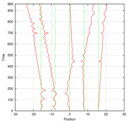
Indeed, let us assume that we know how to split the -dimensional space of our soliton parameters into regions that correspond to the different asymptotic regimes. Obviously, if we choose the soliton parameters to be close to the ‘border’ between two different regimes we can expect that we would have a ‘transition’ area between the regimes, so the deviation from the CTC model will come up sooner than 1000. This is what we can see in the right panels of Figures 2, 3. There for we see that the bound state of 5 solitons in fact transforms into a MAR. The first and the fifth solitons ‘peel off’ and go freely away, and the other three still stay in a BSR. It seems that increasing the differences between the amplitudes stabilizes the BSR.
The general criterium that ensures FAR or BSR is based on the following well known proposition coming from linear algebra.
Proposition 1
Let be symmetric matrix with real-valued matrix elements. Then its eigenvalues will be real and different, i.e., for .
Corollary 1
Let be symmetric (not hermitian) matrix with purely imaginary matrix elements. Then its eigenvalues will be purely imaginary and different, i.e., for .
Proof 1
Follows directly from the Proposition if we consider .
In addition below we will assume that and .

3.2 Generic FAR Configurations
In what follows we choose the polarization vectors by setting:
| (24) |
where , or .
For the CTC using the Proposition we obtain:
| (25) |
which means that
| (26) | ||||
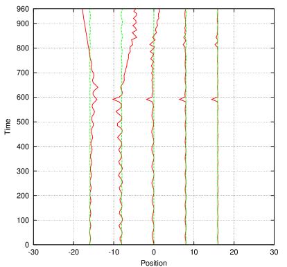
Indeed, from the Proposition the eigenvalues of will be real and different, which is FAR. A particular case of (26) as configuration ensuring FAR for scalar solitons was noticed long ago, namely choosing solitons with equal amplitudes (i.e., ) and and out-of phase [4]. However, eq. (26) provides more general configurations, in which the solitons may have non-vanishing initial velocities, see Figure 1.

3.3 Generic BSR Configurations
Here we use the Corollary and impose on the conditions:
| (27) |
which means that
| (28) | ||||
This is also rather general and simple condition on the soliton parameters that fixes the initial velocities to be 0, but does not put restrictions (except the adiabatic ones) on the amplitudes and on the initial positions of the solitons.
3.4 Symmetric Configurations of Soliton Parameters
In addition to these we find other configurations of soliton parameters that provide FAR or BSR. To this end we use special symmetric constraints on described below. These constraints will leave only one of and independent. As a result the characteristic polynomial of will factorize and we will find that all roots are proportional to each other.
Let us give few examples of them. We will provide the corresponding Lax matrix, its characteristic polynomial and eigenvalues.
-
•
, :
(29) -
•
,
(30) -
•
,
(31) 
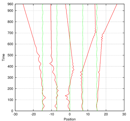
Figure 3: Left panel: FAR with initial conditions , , ; Right panel: BSR with initial conditions , , . The rest of the parameters are defined by eqs. (38) and (39) respectively. -
•
, :
(32)
Such examples can be found for any value of ; from algebraic point of view they are related to the the maximal embedding of as a subalgebra of .
In order to ensure FAR or BSR we need to impose on and the condition that
| (33) |
Initial conditions for BSR of 5 scalar solitons:
| (34) | ||||||||||||
Initial conditions for FAR of 5 scalar solitons:
| (35) | ||||||||||||
For Manakov solitons the initial positions are determined by:
| (36) | ||||||
For the numerics we again fix the polarization vectors as in (24) and evaluate by the formula (36). The result is:
| (37) |
In order to have FAR we choose the amplitudes, velocities and the phases of the solitons by:
| (38) | ||||||||
For the BSR we choose the amplitudes, velocities and the phases of the solitons by:
| (39) | ||||||||
3.5 Numeric Values for the Initial Parameters
In the Tables we list the numeric values for and for the two typical choices of and used above.
| left panel | right panel | |
|---|---|---|
| 0.0 | 0.0 | |
| 2.868037 | -0.273554 | |
| -0.405708 | -0.405708 | |
| 2.781038 | -0.360554 | |
| -0.150741 | -0.150741 |
| left panel | right panel | |
|---|---|---|
| 0.0 | 0.0 | |
| 2.484841 | -0.656751 | |
| -1.006917 | -1.006917 | |
| 2.258187 | -0.883405 | |
| -0.354039 | -0.354039 |
| left panel | right panel | |||
|---|---|---|---|---|
| 0.0 | -15.154654 | 0.0 | -15.154654 | |
| 2.484841 | -7.133487 | -0.656751 | -7.133487 | |
| -1.006917 | .140982 | -1.006917 | 0.140982 | |
| 2.258187 | 7.305540 | -0.883405 | 7.305540 | |
| -.354039 | 15.154654 | -0.354039 | 15.154654 | |
Conclusions and Discussion
The above analysis can be extended to any number of solitons. As we mentioned above, the symmetric Lax matrices are realizations of the maximal embedding of the algebra as a subalgebra of . In this case we effectively reduce the -soliton interactions to an effective -soliton interactions. Therefore the symmetric configurations studied above allow only two asymptotic regimes: BSR and FAR. We make the hypothesis that it would be possible to construct more general symmetric Lax matrices that would be responsible for effective -soliton interactions. In this paper we included numerical tests only for 3 soliton interactions. However previously we have run test starting with 2-solitons and ending with 9-soliton configurations. Our results are that the CTC models adequately not only the purely solitonic interactions, but also the effects of external potentials and other perturbations on them.
An interesting question is how long should we wait for the asymptotic regime. This question is directly related to the other one: What are the limits of applicability of CTC? In our simulations we have chosen which means that the asymptotic time must be of the order of . At the same time in a number of cases we find good match between the CTC and the numeric solutions of Manakov model even until . This is what we see in our tests in this paper for the free asymptotic regimes (right panels of all Figures). The situation is different for the bound state regimes. While in Figure 1 we see good match until about 700, in Figures 1 and 3 the good match goes until 300. After that the trajectories of CTC keep to the BSR, but some of the real solitons ‘escape aeay‘ after that. However in all cases we find that CTC provides good descriptions until times about three times larger than the asymptotic one.
Acknowledgements
MDT was supported by Fulbright – Bulgarian-American Commission for Educational Exchange under Grant No 19-21-07.
References
- [1] F. Kh. Abdullaev, B. B. Baizakov, S. A. Darmanyan, V. V. Konotop, M. Salerno. Nonlinear excitations in arrays of Bose-Einstein condensates. Phys. Rev. A64, 043606 (2001).
- [2] G. P. Agrawal, Nonlinear Fiber Optics, (Academic, San Diego, 1995) (2nd edn).
- [3] D. Anderson, and M. Lisak. Bandwidth limits due to mutual pulse interaction in optical soliton communication systems. Optics Lett. 11, 174 (1986).
- [4] J. M. Arnold. Complex Toda lattice and its application to the theory of interacting optical solitons. JOSA A 15A (1998) 1450–1458.
- [5] J. M. Arnold. Stability of solitary wave trains in Hamiltonian wave systems. Phys. Rev. E60 (1999) 979–986.
- [6] R. Carretero-Gonzales, V. S. Gerdjikov, M. D. Todorov. “-soliton interactions: Effects of linear and nonlinear gain/loss.” AIP CP1895, 040001, 10p (2017).
- [7] R. Carretero-Gonzalez, K. Promislow. Localized breathing oscillations of Bose-Einstein condensates in periodic traps. Phys. Rev. A66, 033610 (2002).
- [8] E. V. Doktorov, V. S. Shchesnovich. Modified nonlinear Schrödinger equation: Spectral transform and N-soliton solution. J. Math. Phys. 36, 7009 (1995).
- [9] H. Flaschka. The Toda lattice. II. Existence of integrals. Phys. Rev. B9, 1924 (1974).
- [10] V. S. Gerdjikov. “-Soliton interactions, the Complex Toda chain and stability of NLS soliton trains.” In: Prof. E. Kriezis (Ed), Proceedings of the International Symposium on Electromagnetic Theory, vol. 1, pp. 307–309 (Aristotle University of Thessaloniki, Greece, 1998);
- [11] V. S. Gerdjikov. “Complex Toda chain – an integrable universal model for adiabatic -soliton interactions.” In: M. Ablowitz, M. Boiti, F. Pempinelli, B. Prinari (Eds), “Nonlinear Physics: Theory and Experiment. II” World Scientific, pp. 64 (2003).
- [12] V. S. Gerdjikov. Modeling soliton interactions of the perturbed vector nonlinear Schrödinger equation. Bulgarian J. Phys. 38 274–283 (2011).
- [13] V. S. Gerdjikov, B. B. Baizakov, M. Salerno. Modelling adiabatic -soliton interactions and perturbations. Theor. Math. Phys. 144(2) 1138–1146 (2005).
- [14] V.S. Gerdjikov, E.V. Doktorov, N. P. Matsuka. -soliton train and generalized Complex Toda chain for Manakov system. Theor. Math. Phys. 151(3), 762–773 (2007).
- [15] V. S. Gerdjikov, E. V. Doktorov, J. Yang. Adiabatic interaction of ultrashort solitons: Universality of the Complex Toda chain model. nlin.SI/0104022; Phys. Rev. E64, 056617 (2001).
- [16] V. S. Gerdjikov, E. G. Evstatiev, D. J. Kaup, G. L. Diankov, I. M. Uzunov. Stability and quasi-equidistant propagation of NLS soliton trains. Phys. Lett. A241, 323–328 (1998).
- [17] V. S. Gerdjikov, D. J. Kaup, I. M. Uzunov, E. G. Evstatiev. Asymptotic behavior of -soliton trains of the Nonlinear Schrödinger equation. Phys. Rev. Lett. 77, 3943–3946 (1996).
- [18] V. S. Gerdjikov, N.A. Kostov, E.V. Doktorov, N.P. Matsuka. Generalized Perturbed Complex Toda chain for Manakov system and exact solutions of the Bose-Einstein mixtures. Mathematics and Computers in Simulation 80, 112–119 (2009); doi:10.1016/j.matcom.2009.06.013. Special Issue of the Journal: “Nonlinear Waves: Computation and Theory.”
- [19] V. S. Gerdjikov, A. V. Kyuldjiev, M. D. Todorov. Manakov solitons and effects of external potential wells. DCDS Supplement Vol.2015, 2015 pp. 505–514.
- [20] V. S. Gerdjikov, M. D. Todorov. “On the effects of sech-like potentials on Manakov solitons.” AIP CP1561, pp. 75–83, (Melville, NY, 2013).
- [21] V. S. Gerdjikov, M. D. Todorov, and A. V. Kyuldjiev. “Polarization effects in modeling soliton interactions of the Manakov model.” AIP CP1684, 080006 (2015); https://doi.org/10.1063/1.4934317.
- [22] V. S. Gerdjikov, M. D. Todorov, A. V. Kyuldjiev. Adiabatic interactions of Manakov soliton – effects of cross-modulation. Special Issue of Wave Motion “Mathematical modeling and physical dynamics of solitary waves: From continuum mechanics to field theory,” Ivan C. Christov, Michail D. Todorov, Sanichiro Yoshida (Eds), Wave Motion 71 71–81 (2017); ArXiv:1610.08413v1[nlin.SI].
- [23] V. S. Gerdjikov, I. M. Uzunov. Adiabatic and non-adiabatic soliton interactions in nonlinear optics. Physica D 152-153, 355–362 (2001).
- [24] V. S. Gerdjikov, I. M. Uzunov, E. G. Evstatiev, G. L. Diankov. Nonlinear Schrödinger equation and -soliton interactions: Generalized Karpman-Solov’ev approach and the Complex Toda chain. Phys. Rev. E55(5), 6039–6060 (1997).
- [25] V. I. Karpman. Soliton evolution in the presence of perturbation. Physica Scripta 20 (1979) 462–478.
- [26] V. I. Karpman, V. V. Solov’ev. A perturbational approach to the two-soliton systems. Physica D3D, 487, (1981).
- [27] Yu. S. Kivshar, B. A. Malomed. Dynamics of solitons in nearly integrable systems. Rev. Mod. Phys. 61(4), 763–915 (1989).
- [28] S. V. Manakov. On the theory of Two-dimensional stationary self-focusing electromagnetic waves. JETPh 65 (1973) 505–516; English translation: Sov. Phys. JETP 38 (1974) 248–253.
- [29] S. V. Manakov. On the complete integrability and stochastization in discrete dynamical systems. Sov.Phys. JETP 40, (1974) 269–274.
- [30] Midrio, Wabnitz, Franco. Perturbation theory for coupled nonlinear Schrödinger equations. Phys. Rev. E54, 5743 (1996).
- [31] J. Moser. In: Dynamical Systems, Theory and Applications. Lecture Notes in Physics, v. 38 (Springer Verlag, 1975), p. 467.
- [32] V. S. Shchesnovich, E. V. Doktorov. Perturbation theory for the modified nonlinear Schr dinger solitons. Physica D 129, 115 (1999).
- [33] M. D. Todorov, V. S. Gerdjikov, A. V. Kyuldjiev. Multi-soliton interactions for the Manakov system under composite external potentials. Proc. Estonian Academy of Sciences, Phys.-Math. Series. 64(3), 368 -378 (2015).
- [34] I. M. Uzunov, M. Gölles, F. Lederer. Stabilization of soliton trains in optical fibers in the presence of third-order dispersion. JOSA B12(6), 1164 (1995).
- [35] V. E. Zakharov, S. V. Manakov, S. P. Novikov, L. P. Pitaevskii. Theory of Solitons: The Inverse Scattering Method (Plenum, N.Y., Consultants Bureau, 1984).
- [36] V. E. Zakharov and A. B. Shabat. Exact theory of two-dimensional self-focusing and one-dimensional self-modulation of waves in nonlinear media. Zh. Eksp. Teor. Fiz. 61 (1971) 118–134.