Homogeneous isotropic turbulence in four spatial dimensions

Abstract

Direct Numerical Simulation is performed of the forced Navier-Stokes equation in four spatial dimensions. Well equilibrated, long time runs at sufficient resolution were obtained to reliably measure spectral quantities, the velocity derivative skewness and the dimensionless dissipation rate. Comparisons to corresponding two and three dimensional results are made. Energy fluctuations are measured and show a clear reduction moving from three to four dimensions. The dynamics appear to show simplifications in four dimensions with a picture of increased forward energy transfer resulting in an extended inertial range with smaller Kolmogorov scale. This enhanced forwards transfer is linked to our finding of increased dissipative anomaly and velocity derivative skewness.

I Introduction

Turbulence is considered the oldest unsolved problem of theoretical physics. Moreover, the difficulty of the problem is such that it is still unknown if solutions to the underlying three dimensional Navier-Stokes equations (NSE) can exhibit singularities in finite time. In recent years, major advances have been made in understanding the turbulent behavior of the NSE using direct numerical simulation (DNS). In some ways this success has diverted efforts in physics from understanding the underlying structure of this equation in which a solution to the problem of turbulence may lie.

In this paper, we shed new light on the properties of the NSE by utilizing DNS to study this equation in four spatial dimensions. A common tool of theoretical physics is to examine systems under different conditions, in our case the spatial dimension, in order to obtain new insights. We report the first results of fully developed statistically stationary turbulence in 4D, building on the work of Gotoh et al.gwsns07 who performed simulations of free decay. Through a comprehensive dataset that spans a significant region of parameter space we aim to provide phenomenological insights into the connection between turbulence dynamics and dimensionality in the wider context of complex systems. Fluctuation and dissipation are quantities typically studied in understanding complex systems of many degrees of freedom, and in this paper we will make one new measurement of each in 4D, to add to our general knowledge about turbulence.

Before explaining the necessary technical details and the numerical results, we provide a summary of existing works on the subject of dimensionality in turbulence, with the aim of raising interest in the subject from the wider theoretical physics community. Investigations have been conducted for the mathematical structure of the NSE in higher spatial dimensions scheffer ; dong1 ; dong2 ; dong3 ; guo . In the study of fully developed turbulence, the role of the spatial dimension has been an area of sustained focus. This has been particularly true ever since the development of renormalization group methods and their successful application to critical phenomena by Wilson and Fisher wf72 ; wilson83 ; fisher98 . These problems, as well as quantum field theory, share a number of common features. Of central importance is the presence of a large number of degrees of freedom across a range of length scales, which are often strongly interacting. As such, fluctuations, which may be present over many of these length scales, play a crucial role in these systems. In the case of critical phenomena, the connection between dimensionality and the suppression of fluctuations was understood by the Wilson-Fisher fixed point wf72 at four spatial dimensions, though there was also earlier work, such as by Ginzburg ginzburg60 , pointing to the relevance of $D=4$.

The success of this work in the early 1970s led to the application of the same renormalization group ideas to many other systems in physics. For the case of turbulence, this dates back to the work by Forster, Nelson, and Stephens fns76 ; fns77 and DeDominicis and Martins dm79 . These initial works motivated renormalization-group techniques as a means to treat the multi-scale physics of turbulence. Embedded in this approach, the spatial dimension parameter is a prevalent feature and many subsequent studies have examined how the fixed point properties depend on it fournier ; yakhot ; teodorovich ; eyink1 ; zhou ; berera1 .

The connection between turbulence and quantum field theory extends beyond just the development of the renormalization group. In early work by Kraichnan kraichnan59 , Wyld wyld61 , and Edwards edwards64 , quantum field theory methods were utilized to develop a perturbation theory for the Navier-Stokes equation. Subsequently, notable works by Martin, Siggia, and Rose msr73 using a Hamiltonian approach, and by Jensen jensen81 using a functional integral approach, and many others kawasaki ; mcomb1 ; deker ; phythian ; janssen ; andersen ; berera2 ; frederiksen , continued developing perturbation expansions of the NSE, all borrowing ideas from quantum field theory.

Associations between turbulence and gauge theories have also been made. Quantum Chromodynamics (QCD) is one example. The confinement problem of QCD has similarities to turbulence, due to both having many degrees of freedom involving multi-scale physics, and in addition both are strong coupling problems. One of the first lattice gauge theory simulations by Creutz examined the dependence of QCD on dimensionality Creutz:1979dw , with qualitative differences found in confinement behavior in four versus three spatial dimensions. The QCD connection to turbulence was greatly enhanced by the works of Migdal migdal ; migdal2 ; migdal3 , in developing an analog for the Navier-Stokes equation to the Wilson loop of gauge theories Wilson:1974sk , and Polyakov polyakov1 ; polyakov2 ; polyakov3 ; polyakov4 , in using conformal field theory (CFT) methods to study two-dimensional turbulence, with connections also made between turbulence and the ADS/CFT correspondence maldacena ; fluidgrav ; adscftturb . From another direction, the scaling exhibited by the asymptotically free ultraviolet behavior of QCD has been noted to have similarities to scaling in turbulence eg1994 . Also, the Galilean invariance of the Navier Stokes equation has been interpreted as a gauge invariance abdh1 ; abdh2 .

Motivated from these various directions, there have been many theoretical studies examining the dependence on spatial dimensionality of turbulence. Some have explicitly developed analogies between turbulence and critical phenomena, and through that the possibility of a critical dimension for turbulence eg1994 ; bramwell ; aji ; nelkin1 ; frisch1 ; yakhot2 ; lvov ; giuliani ; frisch3 ; n74 ; nb78 ; fsn78 ; ff78 ; lk97 , above which the Kolmogorov theory (K41) k41 may become exact. Following this line of reasoning, studying turbulence between two and three spatial dimensions reveals a change in energy cascade directions ff78 ; nelkin1 ; frisch1 ; yakhot2 ; lvov ; giuliani ; frisch3 . This has been associated with a lower critical dimension existing at a non-integer intermediate dimension close to $D=2$. Numerical celani ; benavides ; alexakis1 and experimental xia2011 results show that cascade directions can indeed change as a function of different control parameters, one of which being the aspect ratio of the domain . Additionally, the behavior of passive scalars in higher dimensional turbulence has also been investigated kraichnan1974scalar , and here it was found that for a certain prescribed velocity field intermittency vanished in the $d\rightarrow\infty$ limit. Furthermore, studies above three dimensions n74 ; nb78 ; fsn78 ; ff78 ; khesin ; kraichnan1994a ; ffr have made various claims as to the extent turbulent behavior changes at higher dimensions. Kraichnan k85 and Meneveau and Nelkin mn89 predict a change in inertial range behavior at spatial dimension $D=4$. Further to this, Liao liao90 ; liao91 and Nelkin nelkin03 argue, through close analogies to critical phenomena, for an upper critical spatial dimension of six and four respectively for turbulence. Similarities between the NSE and the Kardar-Parisi-Zhang (KPZ) equation have also been observed lk97 due to both having nonlinear strong coupling regimes. In the latter, it has been theoretically argued that four spatial dimensions is a type of critical dimension, whether a corresponding result exists for the NSE is left as an interesting question. More recently a study ffo10 of fluid velocity correlation functions in varying dimensions highlighted competing effects on the statistics. This work gave some analytic relations but left essential open questions requiring numerical study.

From this short review, it is clear that understanding the dependence of turbulent behavior in the NSE on spatial dimension has been an area of sustained interest for at least the past half century. Theoretical considerations and speculations are abundant, with many analogies made to critical phenomena and quantum field theory, where it is already an established fact that spatial dimensionality plays a significant role in governing behavior. These theoretical treatments provide strong motivation to numerically study the properties of turbulence in spatial dimensions higher than three. This is a very computationally expensive challenge, though computing power has reached a stage where meaningful studies can now be performed.

Previous investigations into higher dimensional turbulence via DNS have been insightfully motivated but limited in scope Suzuki2005 ; gwsns07 ; ysing12 ; nikitin11 . All four of these studies were for freely decaying turbulence, with short run times and relatively coarse grid spacing, a restriction imposed by the available computing power at that time. The maximum grid resolution in any direction was 256 collocation points, which in 3D is not sufficient to result in a scaling region for free decay, with at least 512 being a safe minimum. For example, the scaling reported in Suzuki2005 ; gwsns07 ; ysing12 was based on normalization of the energy spectra, which has its ambiguities in capturing the scaling regime. Moreover the short simulation times in all four papers gwsns07 ; ysing12 ; nikitin11 increases the risk of being influenced by the effect of the initial conditions on the statistics. Nevertheless, these papers presented the first measurements of important observables in turbulence such as energy spectra, the skewness of velocity-field gradients and energy decay rates in 4D turbulence to the best possible accuracy permitted by computing power at that time. All these groundbreaking simulations were done some time ago. What is needed and possible now are larger, stationary state, simulations. Although this is computationally intensive, it is necessary if the data are to be reliable and not rely on external assumptions. In this paper we are able to go to large enough box size and evolution time in forced simulations to report the first fully-developed turbulence datasets in 4D. Moreover the past 4D DNS studies placed considerable focus on intermittency properties. Our paper is following a different physical motivation, that of turbulence as an example of a strong coupling problem. It is in that context we presented examples in this Introduction from critical phenomenon and quantum field theory, with turbulence yet being another example of a strongly coupled theory.

II Basic equations

In this study we look systematically at forced DNS in two, three, and four spatial dimensions. In such simulations, a steady state is reached which allows for a clear scaling regime to be identified, with statistics taken for multiple large eddy turnover times and performed on up to $512^{4}$ collocation points. Obtaining such a large dataset is a non-trivial task, but is necessary to reach a level where the spectral quantities and correlations typically associated with turbulence can be reliably measured. By doing so it is possible to make direct comparison to turbulence in two and three spatial dimensions.

The Navier-Stokes equations

$$\begin{split}\partial_{t}u_{i}+u_{j}\Omega_{ji}&=-\partial_{i}\left(P+\frac{u^{2}}{2}\right)+\nu\nabla^{2}u_{i}+f_{i}\ ,\\ \partial_{i}u_{i}&=0\ ,\end{split}$$ (1)

are numerically integrated using a fully de-aliased pseudo-spectral code in a periodic cube of length $2\pi$ YoffeThesis ; EddyBurgh . Here, $\bm{u}(\bm{x},t)$ is the velocity field, $P(\bm{x},t)$ is the pressure field, $\nu$ is the kinematic viscosity, $\bm{f}(\bm{x},t)$ is an external force and $\Omega_{ij}=\partial_{i}u_{j}-\partial_{j}u_{i}$ is the vorticity 2-form. The density was set to unity. Equation (1) is equivalent to the standard form in all dimensions.

For fluid flows of any dimension, inviscid invariants exist depending on whether the spatial dimension is odd or even, referred to as helicity-type and enstrophy-type invariants respectively invar4d . Thus, to ensure the correctness of our four-dimensional NSE implementation, we measured the lowest order invariant and found it was indeed conserved in the non-linear term.

The primary forcing used was a negative damping scheme which only forced the low wave numbers (large scales), $k_{f}=2.5$, according to the rule

$$\boldsymbol{\hat{f}}(\boldsymbol{k},t)=\begin{cases}(\varepsilon/2E_{f})\boldsymbol{\hat{u}}(\boldsymbol{k},t)\quad&\text{if }0<k\leq k_{f},\\ 0\qquad&\text{else,}\end{cases}$$ (2)

where $E_{f}$ is the energy in the forcing band $0<k\leq k_{f}$ and $\bm{\hat{u}}(\bm{k},t)$ is the Fourier transform of field $\bm{u}$. This well tested forcing function force ; Kaneda2006 ; Linkmann2015 allows the dissipation rate, $\varepsilon$, to be known a priori. We set $\varepsilon$ to 0.1 for all runs. The simulations were well resolved, with $k_{\text{max}}\eta>1$ for all simulations, where $k_{\text{max}}$ is the largest wavenumber in the simulation and $\eta$ the Kolmogorov microscale. Simulations were initialized randomly from a Gaussian distribution with zero mean.

The pseudo-spectral technique allows statistics of the field to be calculated from the energy spectra. Due to the properties of homogeneity and isotropy, the calculations depend on the spatial dimension of the field. In D-dimensional homogeneous isotropic turbulence $u$, the rms velocity, is defined as $u=\sqrt{2E/D}$, where $D$ is the spatial dimension and $E$ the energy. The integral length scale, $L_{D}$, and Taylor microscale, $\lambda_{D}$, are calculated from simulations as

$$\begin{split}L_{D}&=\frac{\Gamma(\frac{D}{2})\sqrt{\pi}}{\Gamma(\frac{D+1}{2})u^{2}}\int_{0}^{\infty}\mathrm{d}k\,E(k)k^{-1}\ ,\\ \lambda_{D}&=\sqrt{\frac{D(D+2)\nu u^{2}}{\varepsilon}}\;,\end{split}$$ (3)

where $E(k)$ is the energy spectrum. The Reynolds numbers quoted throughout the paper are then the integral scale Reynolds number $\mathrm{Re}_{L}=uL_{D}/\nu$ and the Taylor Reynolds number $\mathrm{Re}_{\lambda}$ = $u\lambda_{D}/\nu$. Due to their dependence on the spatial dimension it is important the correct form is used, particularly for determining the scaling properties of the velocity derivative skewness as well as for measuring the correct value for the dimensionless dissipation rate.

ReL	Reλ	$T_{0}$	$\nu$	$L$	$\lambda$	$U$	$k_{\mathrm{max}}$	$\eta$
160	74	2.31	0.0008	0.54	0.080	0.24	169	0.0842
225	94	1.80	0.0008	0.57	0.080	0.32	169	0.0824
248	72	5.18	0.0002	0.51	0.039	0.10	340	0.0350
276	108	1.56	0.0008	0.59	0.080	0.38	169	0.0692
319	124	1.37	0.0008	0.59	0.080	0.43	169	0.0684
358	131	1.29	0.0008	0.61	0.080	0.47	169	0.0604
626	171	1.68	0.0003	0.56	0.049	0.33	340	0.0456
633	155	2.34	0.0002	0.54	0.038	0.23	340	0.0245
676	167	2.16	0.0002	0.54	0.040	0.25	340	0.0420
696	139	3.78	0.0001	0.51	0.027	0.14	340	0.0206
698	186	1.54	0.0003	0.57	0.049	0.37	340	0.0404
823	193	1.85	0.0002	0.55	0.040	0.30	340	0.0385
945	217	1.62	0.0002	0.55	0.040	0.34	340	0.0397
966	188	2.77	0.0001	0.52	0.028	0.19	340	0.0378
984	196	1.78	0.0002	0.59	0.040	0.33	340	0.0271
1054	231	1.53	0.0002	0.57	0.040	0.37	340	0.0355
1157	242	1.45	0.0002	0.58	0.040	0.40	340	0.0320
1180	223	2.32	0.0001	0.52	0.028	0.23	340	0.0297
1318	225	2.29	0.0001	0.55	0.028	0.24	340	0.0192
1360	246	2.09	0.0001	0.53	0.028	0.26	340	0.0284
1488	259	1.98	0.0001	0.54	0.028	0.27	340	0.0275
1659	277	1.82	0.0001	0.55	0.028	0.30	340	0.0286
1696	268	2.13	0.00008	0.54	0.025	0.25	681	0.0271
1915	304	1.67	0.0001	0.57	0.028	0.34	340	0.0257
1954	276	2.70	0.00005	0.51	0.020	0.19	681	0.0262
1985	297	1.69	0.0001	0.58	0.027	0.34	340	0.0154
2026	336	1.51	0.0001	0.55	0.028	0.37	340	0.0265
2241	350	1.44	0.0001	0.57	0.028	0.39	340	0.0257
3274	352	2.73	0.00003	0.52	0.015	0.19	681	0.0176
3900	378	2.78	0.000025	0.52	0.014	0.19	681	0.0168
4925	435	2.69	0.00002	0.52	0.013	0.19	681	0.0151
9831	610	2.73	0.00001	0.52	0.009	0.19	681	0.0106
19485	878	2.69	0.000005	0.51	0.006	0.19	1364	0.0069

Table 1: Simulation parameters for 2D runs. Due to the inverse energy cascade a hypoviscous term, proportional to $\nabla^{-2}$, was utilized to prevent condensation at the largest scales. For all runs the sum of large and small scale energy dissipation was 0.1. Here $\eta=\left(\nu^{3}/\varepsilon_{\omega}\right)^{1/6}$, where $\varepsilon_{\omega}$ is the enstrophy dissipation rate.

ReL	Reλ	$T_{0}$	$\nu$	$L$	$\lambda$	$U$	$k_{\mathrm{max}}$	$\eta$
11	9	4.81	0.08	2.10	1.51	0.44	20	0.2675
11	9	4.78	0.09	2.20	1.69	0.46	20	0.2922
13	11	4.60	0.07	2.08	1.46	0.45	20	0.2420
15	11	4.29	0.06	1.93	1.35	0.45	20	0.2156
23	16	3.71	0.04	1.85	1.22	0.50	20	0.1591
30	20	3.32	0.03	1.74	1.11	0.52	20	0.1282
45	27	2.97	0.02	1.63	0.95	0.55	20	0.0946
46	29	2.94	0.02	1.64	0.97	0.56	169	0.0946
75	39	2.42	0.01	1.34	0.68	0.55	20	0.0562
88	44	2.39	0.009	1.37	0.67	0.57	41	0.0520
88	44	2.57	0.01	1.50	0.72	0.58	169	0.0562
96	47	2.32	0.008	1.33	0.63	0.57	41	0.0476
112	51	2.28	0.007	1.34	0.60	0.59	41	0.0430
130	57	2.19	0.006	1.31	0.57	0.60	41	0.0383
147	61	2.02	0.005	1.22	0.52	0.60	169	0.0334
153	63	2.15	0.005	1.28	0.52	0.60	41	0.0334
201	73	2.12	0.004	1.31	0.48	0.61	41	0.0283
249	83	2.05	0.003	1.24	0.41	0.60	84	0.0228
344	100	1.82	0.002	1.12	0.34	0.62	169	0.0168
378	103	1.98	0.0019	1.19	0.32	0.60	84	0.0162
393	107	2.05	0.002	1.27	0.34	0.62	84	0.0168
395	108	1.94	0.0018	1.17	0.31	0.61	84	0.0155
436	113	1.99	0.0017	1.22	0.31	0.61	84	0.0149
484	120	2.02	0.0016	1.25	0.30	0.62	84	0.0142
488	121	1.96	0.0015	1.20	0.29	0.61	84	0.0136
536	125	1.98	0.0014	1.22	0.28	0.62	84	0.0129
806	158	2.01	0.001	1.27	0.24	0.63	169	0.0100
979	174	1.97	0.0008	1.24	0.22	0.63	169	0.0085
1096	180	1.85	0.0006	1.10	0.18	0.60	169	0.0068
1446	212	1.86	0.0005	1.16	0.17	0.62	340	0.0059
2517	286	1.87	0.0003	1.19	0.13	0.64	340	0.0041
6207	453	1.75	0.00011	1.09	0.08	0.63	681	0.0019

Table 2: Simulations parameters for 3D runs, $\varepsilon=0.1$ for all cases.

ReL	Reλ	$T_{0}$	$\nu$	$L$	$\lambda$	$U$	$k_{\mathrm{max}}$	$\eta$
27	15	4.99	0.03	2.01	1.12	0.40	20	0.130
39	20	4.42	0.02	1.87	0.95	0.42	20	0.096
52	24	4.12	0.015	1.79	0.84	0.44	20	0.077
74	31	3.74	0.01	1.66	0.70	0.45	41	0.057
99	38	3.70	0.008	1.71	0.65	0.46	41	0.048
126	44	3.50	0.006	1.63	0.56	0.47	41	0.038
141	46	3.36	0.005	1.54	0.51	0.46	41	0.034
203	57	3.28	0.0035	1.53	0.43	0.47	84	0.026
347	77	3.13	0.002	1.47	0.33	0.47	84	0.017
838	124	2.94	0.0008	1.41	0.21	0.48	169	0.008

Table 3: Simulations parameters for 4D runs, $\varepsilon=0.1$ for all cases.

III Results

In total, we carried out 10 simulations in 4D for $27\leqslant\mathrm{Re}_{L}\leqslant 838$ on $64^{4}-512^{4}$ grid points, 27 runs in 2D with $160\leqslant\mathrm{Re}_{L}\leqslant 19485$ on $512^{2}-4096^{2}$ grid points, and used a 3D dataset BereraPRL containing of 33 runs with $11\leqslant\mathrm{Re}_{L}\leqslant 6207$ on $64^{3}-2048^{3}$ grid points. For more detailed information about the simulations performed see Tables 1, 2 and 3 for 2D, 3D and 4D respectively. These tables should be compared with table 1 in gwsns07 , although caution may be needed as it is not clear if the dimensional corrections to the Taylor length scale have been considered there. Nonetheless, it is clear from these tables that the 4D simulations presented here are at a higher resolution and Re_λ than any work to date. Furthermore, as we make use of a large scale forcing term our results are for statistically stationary turbulence, as such, we can be confident that our measurements pertain to fully developed turbulence which is not true of the decaying runs performed in gwsns07 . In achieving fully developed turbulence our results allow the nature of 4D turbulence, and how it differs from the 3D case, to be understood and allows for theoretical ideas to be tested reliably.

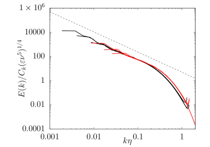
Figure 1: (Color online) Normalized energy spectrum, $E(k)$, against $k\eta$ at Re_L = 6207, 2517 and 979 for 3D (black) and Re_L = 838, 347 and 203 for 4D (red). Kolmogorov $k^{-5/3}$ predicted inertial range scaling (long-dashed black).

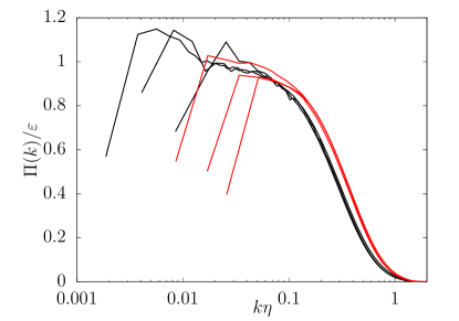
Figure 2: (Color online) Normalized energy flux, $\Pi(k)$ against $k\eta$ at Re_L = 6207, 2517 and 979 for 3D (black) and Re_L = 838, 347 and 203 for 4D (red).

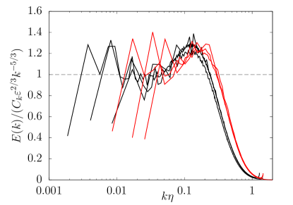
Figure 3: (Color online) Log-linear plot of compensated energy spectrum, $E(k)$, against $k\eta$ at Re_L = 6207, 2517 and 979 for 3D (black) and Re_L = 838, 347 and 203 for 4D (red).

From our simulations, we find that the energy and transfer spectra for 3D and 4D are very similar, and differ from those for 2D (we performed some decaying runs of 4D turbulence and these showed no tendency towards inverse transfer, unlike that found in 2D). In Figures 1 and 2 we show $E(k)$ and $\Pi(k)$, the energy flux, respectively, for a set of 3D (with Re_L from 980 to 6200) and 4D simulations (with Re_L from 200 to 840), which were taken from an ensemble of spectra over multiple large eddy turnover times $T_{0}=L/u$, at intervals longer than $T_{0}$. In Fig. 1, the wave number $k$ is normalized by $\eta$, the energy spectra are normalized with $\epsilon$ and $\nu$ such that they collapse on to the same values in the dissipation range. However, as can be seen in the Figure, the collapse of the spectra only apply if the spatial dimension is the same.

Both 4D and 3D energy spectra are consistent with Kolmogorov $-5/3$ scaling, as can be seen in Fig. 1 and the compensated spectra shown in Fig. 3. The scaling range in 4D is short, as can be expected when considering 3D data at comparable Reynolds numbers. However, we find the Kolmogorov constant, $C_{k}$, to be less in 4D than 3D ,consistent with gwsns07 , with $C_{k}^{\mathrm{3D}}\approx 1.7$ and $C_{k}^{\mathrm{4D}}\approx 1.3$, however, higher resolution simulations are needed to ascertain the true values ishihara2016high . One key difference, highlighted in both plots of the energy flux, Figure 2, and compensated energy spectra, Figure 3, is the existence of a possibly extended scaling region in 4D as compared to 3D, as evidenced by the viscous sub-range beginning at a higher value of $k\eta$ in 4D. This suggests that in this higher dimensional case, there is an increased forward transfer of energy, such that the effects of dissipation do not become dominant until at scales smaller than those in three dimensions. This increase of forward energy transfer with dimension is supported by theoretical predictions, where it is shown to be determined by the possible geometries of triad interactions as the dimension tends to infinity ff78 . Our finding of a stronger forwards transfer is consistent with the larger decay exponent found in gwsns07 . The extended scaling region is in agreement with k85 , which predicts $\eta$ being pushed to smaller values.

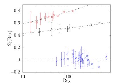
Figure 4: Velocity derivative skewness $S_{0}$ vs Re_λ for two ($\times$), three ($\vartriangle$) and four dimensions ($\square$). The dashed line show least-squares fit to the power law $a$Re${}_{\lambda}^{b}$ as predicted by Kolmogorov’s refined similarity hypothesis. Though this hypothesis was originally formulated for 3D turbulence, given the forward energy cascade present in our 4D simulations it is likely a similar hypothesis could be presented in 4D. The error on the skewness was calculated for less time than other statistics for larger Re_λ

.

To further investigate this enhanced forward transfer, we consider the von Kármán-Howarth equation. From this, it can be shown that the enstrophy equation in 3D takes the form DavidsonBook

$$\begin{split}\partial_{t}Z(t)&=\frac{7}{3}\sqrt{\frac{2}{15}}S_{0}Z(t)^{\frac{3}{2}}-2\nu P(t),\\ S_{0}&=-\frac{\langle(\partial_{x}u_{x})^{3}\rangle}{\langle(\partial_{x}u_{x})^{2}\rangle^{3/2}}\ ,\end{split}$$ (4)

where $S_{0}$ is the negative velocity derivative skewness, $Z(t)$ is the enstrophy and $P(t)$ is the palinstrophy. For example, in 2D there is zero skewness and hence no vortex stretching. From this equation, we see that a larger skewness results in a greater amount of vortex stretching, which may extend to higher dimensions.

In Figure 4 we show $S_{0}$ for 2D, 3D, and 4D. The exact dependence of $S_{0}$ on Re_λ is not known, however, the Kolmogorov 1962 theory K62 predicts $a$Re${}_{\lambda}^{b}$. This is consistent with our data where we find $b^{\mathrm{3D}}=0.08\pm 0.01$ and $b^{\mathrm{4D}}=0.13\pm 0.01$. As such, we find that in four dimensions $S_{0}$ depends more strongly on Re_λ than in three dimensions. As is seen in the plot, 2D has roughly $S_{0}=0$, which is consistent with the absence of vortex stretching. However, in 3D and 4D, $S_{0}$ increases with Re_λ, with skewness higher in 4D than 3D a trend that has been also been observed for free decay gwsns07 . This data also suggests that if, as is predicted by the K41 theory, the skewness takes on a universal value as Re_λ $\rightarrow\infty$ then this asymptotic value is larger in 4D. We can then interpret this larger skewness value in 4D as being indicative of an enhanced rate of enstrophy production. Furthermore, this result can be understood as the extra spatial dimension allowing for additional vortex stretching, and hence an increased forward cascade of energy.

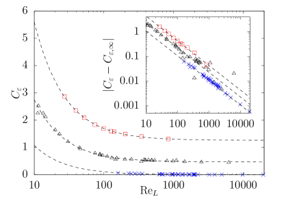
Figure 5: Main panel: $C_{\varepsilon}$ against Re_L. Dashed line fit for model Equation (6) for two ($\times$), three ($\vartriangle$) and four ($\square$) dimensions. Inset: $|C_{\varepsilon}-C_{\varepsilon,\infty}|$ against Re_L, dashed line corresponds to power law behavior.

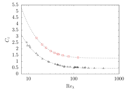
Figure 6: $C_{\varepsilon}(\mathrm{Re}_{\lambda})$ against Re_λ. Dashed line fit for model Equation (7) for three ($\vartriangle$) and four ($\square$) dimensions.

The dissipative anomaly in 3D turbulence, where the rate of energy dissipation tends to a nonzero asymptotic value in the limit of infinite Reynolds number, is one of the fundamental phenomenological characteristics of turbulence. It clearly distinguishes 3D from 2D dynamics and it is connected with mathematical difficulties in proving regularity in the 3D Navier-Stokes equations. The dimensionless dissipation rate is defined as

$$C_{\varepsilon}=\frac{\varepsilon L}{u^{3}}\ ,$$ (5)

There is ample experimental sreenivasan1 ; sreenivasan2 ; burattini and numerical wang1 ; gotoh1 ; donzis ; bos1 ; yeung1 ; yeung2 ; ishihara evidence that, in 3D, $C_{\varepsilon}\to C_{\varepsilon,\infty}\neq 0$ as Re_L $\ \rightarrow\infty$, indicating the persistence of a finite rate of energy dissipation even in the limit of zero viscosity. This is known as the dissipative anomaly and can be understood as being a consequence of vortex stretching Doering2009 and thus of non-zero skewness. The dependence of $C_{\varepsilon}$ on Re_L can be approximately described as Doering2002 ; McComb2015

$$C_{\varepsilon}=C_{\varepsilon,\infty}+\frac{C}{\mathrm{Re}_{L}}\ ,$$ (6)

where $C$ is a constant. A similar result can also be derived Doering2002 ; McComb2015 for $C_{\varepsilon}$ in terms of Re_λ, which gives

$$C_{\varepsilon}(\mathrm{Re}_{\lambda})=A\left[1+\sqrt{1+\left(\frac{B}{\mathrm{Re}_{\lambda}}\right)^{2}}\right],$$ (7)

where $A$ and $B$ are constants with respect to Re_λ.

The value of $C_{\varepsilon,\infty}$ depends on dimensionality and the inviscid invariants, in 3D the high levels of helicity reduce $C_{\varepsilon,\infty}$ Linkmann18 , and in 2D, where there is no forwards cascade of energy, $C_{\varepsilon,\infty}=0$. Hence it is of interest to examine the behavior of $C_{\varepsilon}$ also in 4D. In Figure 5 we show the Re dependence of $C_{\varepsilon}$ for 2D, 3D, and 4D data, and we find that it is well described by Eq. (6) in all cases, albeit with different values of $C_{\varepsilon,\infty}$ and $C$. Consistent with our results showing an enhanced forward cascade, we see an increase in the value of $C_{\varepsilon,\infty}$ with increasing dimension, this grows from 0.467 for 3D in our data to 1.261 for 4D. Since $C_{\varepsilon}$ is defined in terms of $u$ and $L$, which have explicit dimensional dependence, it may have been possible that the increasing value of $C_{\varepsilon,\infty}$ is solely due to changes in these quantities. However, our results for energy spectra and skewness are independent of how length and velocity scales are defined. Furthermore, the increase of $C_{\varepsilon,\infty}$ between 3D and 4D is greater than would be expected if it were solely caused by these dimensional dependences, thus we conclude that the increased asymptotic dissipation rate is a real effect. In Figure 6 we show the dimensionless dissipation rate in terms of Re_λ and find that the constants in equation 7 take on the values $A=0.225342$ and $B=90.0105$ in 3D and $A=0.63123$ and $B=51.0446$ in 4D.

Fluctuations are another important measure for assessing change in behavior. For the case of critical phenomena above the upper critical dimension, mean field theory becomes exact close to the critical point. If there is an upper critical dimension, then there should be true scale invariance in the inertial range. This would result in reduced fluctuations and smaller deviations from the K41 theory in terms of structure functions as we move towards this dimension. At criticality, the two point correlation functions of such systems display scale invariance.

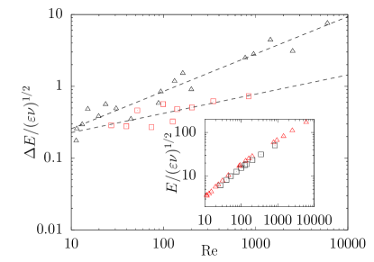
Figure 7: Normalized variation of energy with Re_L in three ($\vartriangle$) and four ($\square$) dimensions. Inset: normalized energy with Re_L at same scale as main plot.

Figure 7 shows a plot of $\Delta E/(\varepsilon\nu)^{1/2}$ with Re_L, where $\Delta E$ is the standard deviation of the total energy in time. This figure shows a measure of the fluctuation with Re_L in 3D and 4D. The dashed line shows a power law fit for illustrative purposes. The fluctuations for 4D are smaller than 3D and rise slower. The inset shows normalized energy with Re_L, with both 3D and 4D data being roughly similar. Thus, the decreased fluctuations are not merely an effect of there being lower total energy. One may also plot $\Delta E/E$ and the 4D case has values clearly lower than the 3D values, with the difference becoming more pronounced at higher Re_L. Another aspect of the simulations which suggests smaller fluctuations for 4D than in 3D, was the tendency of 4D simulations to reach statistically steady states in as little as half the time. Further to this, the fluctuation with wave number of the transfer spectra $T(k)$ were much greater in 3D than 4D (not shown).

IV Concluding remarks

This paper has reported a series of 4D HIT DNS simulations for the forced Navier-Stokes equation. There have only been a few previous DNS simulations in 4D Suzuki2005 ; gwsns07 ; ysing12 ; nikitin11 , all done for free decay. These were groundbreaking papers for this computationally demanding direction, but free decay for the relatively small box sizes they achieved limited the period of fully-developed turbulence to be very short if at all. Our simulations were run for adequately long time and for sufficiently large box sizes to produce for the first time a reliable and robust regime of fully developed turbulence. This now opens the possibility to numerically test theoretical ideas about 4D turbulence with a reliable 4D simulated turbulent state. As discussed at the start of the paper, there is various discussion scattered in the literature over many years on how studying 4D turbulence might shed new insights in the theoretical understanding of turbulence. This work helps move one step further in that direction.

The numerical demands to simulate fully-developed turbulence in 4D limits the extent of measurements that can be achieved. Our results are modest but interesting for two main reasons. Firstly, in 4D we find the presence of a seemingly enhanced forward energy cascade, consistent with what has been suggested in theoretical studies. Our results also show an increase in the asymptotic dimensionless dissipation rate and velocity derivative skewness, which is further evidence of the enhanced forward energy cascade. Secondly, we see a reduction in the size of fluctuations in the total energy when going from three to four dimensions. The reduction of these fluctuations is due to the non-linear transfer of energy between different length scales in the flow, coming from an increased tendency of energy passing from large to small scales. Noting that the reduction in Fig. 7 is on a log-plot, it is quite a dramatic decrease in going from 3D to 4D (as is also the case for $\Delta E/E$ which is not shown but we have checked). Thus turbulence joins critical phenomenon and QCD, as discussed in the Introduction, as another strong coupling, multi-degree of freedom problem that exhibits noteworthy changes from 3D to 4D.

For several decades the question has lingered in the literature as to whether there are any distinct differences to turbulence in three versus four spatial dimensions. The barriers to answering this question have been to identify appropriate quantities to measure and then measure them to adequate computational reliability. The handful of past datasets Suzuki2005 ; gwsns07 ; ysing12 already produced some interesting results that showed differences between three and four dimensions. However these were small datasets for which it is unclear the degree to which they realize fully developed turbulence.

In this work we have identified two measures, one related to dissipation and another to fluctuations, to compared between 3D and 4D turbulence. We have then developed a dataset at adequately high resolution and evolved long enough, so as to realize fully developed turbulence in 4D, from which we could then reliably take measurements of these two quantities. Our results have therefore provided the first definitive measurements of a 4D turbulence state, from which we could demonstrate some clear differences in turbulence between three and four spatial dimensions. We do find some differences in the behavior of turbulence, with, in particular, significant suppression of at least this one measure of fluctuations in four compared to three dimensions.

These measurements are computationally very demanding, as they are in four spatial dimensions, need adequately high spatial and temporal resolution, and require well equilibriated forced simulations. Further definitive measurements of other forms of fluctuation and dissipation behavior in four and even higher dimensions would be of interest. The new insights learned from such efforts may assist in reaching the long sought for theory of turbulence. Nevertheless for now the computational demands place considerable limitations on any rapid progress along these lines.

For instance, the measurements of the velocity-gradient skewness presented in Fig. 4 show that extreme fluctuations in the velocity-field gradients become more likely in 4D than in 3D with increasing Reynolds number and thus at smaller and smaller scale. This motivates fundamental questions concerning self-similarity that are usually assessed in terms of structure function scaling, in particular at high order, where deviations from dimensional scaling are observed in 3D. Such measurements are very challenging in 4D, as they require an extended scaling range in order to be reliable and this highly resolved simulations. Our results provide a first step in this direction and a motivation to take this challenge on.

- (1) V. Scheffer, Comm. Math. Phys. 61, 41 (1978).
- (2) H. Dong and D. Du, Comm. Math. Phys. 273, 785 (2007).
- (3) H. Dong and R. M. Strain, Indiana Uni. Math. J. 61, 2211 (2012).
- (4) H. Dong and X. Gu, J. Func. Analysis 267, 2606 (2014).
- (5) X. L. Guo and Y. Y. Men, Acta Math. Sinica 33, 1632 (2017).
- (6) K. G. Wilson and M. E. Fisher, Phys. Rev. Lett. 28, 240 (1972).
- (7) K. G. Wilson, Rev. Mod. Phys. 55, 583 (1983).
- (8) M. E. Fisher, Rev. Mod. Phys. 70, 653 (1998).
- (9) V. L. Ginzburg, Fiz. Tverd. Tela 2, 2031 (Sov. Phys.-Solid State bf 2, 1824), (1960).
- (10) D. Forster, D. R. Nelson, and M. J. Stephen, Phys. Rev. Lett. 36, 867 (1976)
- (11) D. Forster, D. R. Nelson, and M. J. Stephen, Phys. Rev. A 16, 732 (1977).
- (12) C. DeDominicis and P. C. Martin, Phys. Rev. A 19, 419 (1979).
- (13) J. D. Fournier and U. Frisch, Phys. Rev. A28, 1000 (1983).
- (14) V. Yakhot and S. A. Orszag, Phys. Rev. Lett. 57, 1722 (1986).
- (15) E. V. Teodorovich, Fluid Dynamics 29, 770 (1994).
- (16) G. L. Eyink, Phys. Fluids 6, 3063 (1994).
- (17) Y. Zhou, Physics Reports 488, 1 (2010).
- (18) A. Berera and S. R. Yoffe, Phys. Rev. E82, 066304 (2010).
- (19) R. H. Kraichnan, J. Fluid Mech. 5, 497 (1959).
- (20) H. W. Wyld, Jr., Ann. Phys. 14, 143 (1961).
- (21) S. F. Edwards, J. Fluid Mech. 18, 239 (1964).
- (22) P. C. Martin, E. D. Siggia, and H. A. Rose, Phys. Rev. A 8, 423 (1973).
- (23) R. V. Jensen, J. Stat. Phys. 25, 183 (1981).
- (24) K. Kawasaki, Prog. Theo. Phys. 52, 1527 (1974).
- (25) W. D. McComb, J. Phys. A 7, 632 (1974).
- (26) U. Deker and F. Haake, Phys. Rev. A 11, 2043 (1975).
- (27) R. Phythian, J. Phys. A 8, 1423 (1975).
- (28) H. Janssen, Z. Phys. B23, 377 (1976).
- (29) H. C. Andersen, J. Math. Phys. 41, 1979 (2000).
- (30) A. Berera, M. Salewski, and W. D. McComb, Phys. Rev. E 87, 013007 (2013).
- (31) J. Frederiksen, J. Math. Phys. 58 103303 (2017).
- (32) M. Creutz, Phys. Rev. Lett. 43, 553 (1979) Erratum: [Phys. Rev. Lett. 43, 890 (1979)].
- (33) A. A. Migdal, Mod. Phys. Lett. A6, 1023 (1991); First Landau Institute Summer School 1993 Proceedings, V. P. Mineev Ed., (1993).
- (34) A. A. Migdal, arXiv preprint hep-th/9310088 (1993).
- (35) A. A. Migdal, arXiv preprint hep-th/9303130 (1993).
- (36) K. G. Wilson, Phys. Rev. D 10, 2445 (1974).
- (37) A. M. Polyakov, arXiv preprint (1992).
- (38) A. M. Polyakov, Nucl. Phys. B396, 367 (1993).
- (39) A. M. Polyakov, Phys. Rev. E52, 6183 (1995).
- (40) S. Boldyrev, T. Linde, A. Polyakov, Phys. Rev. Lett. 93, 184503 (2004).
- (41) Maldacena, Juan, International journal of theoretical physics 38, 1113–1133 (1999).
- (42) Bhattacharyya, Sayantani and Loganayagam, R and Minwalla, Shiraz and Nampuri, Suresh and Trivedi, Sandip P and Wadia, Spenta R, Journal of High Energy Physics 02, 018 (2009).
- (43) Adams, Allan and Chesler, Paul M and Liu, Hong, Phys. Rev. Lett. 112, 151602 (2014).
- (44) G. Eyink and N. Goldenfeld, Phys. Rev. E 50, 4679 (1994).
- (45) A. Berera and D. Hochberg, Phys. Rev. Lett. 99, 254501 (2007);
- (46) A. Berera and D. Hochberg Nucl. Phys. B 814, 522 (2009).
- (47) S. T. Bramwell, P. C. Holdsworth, and J. F. Pinton, Nature 396, 552 (1998).
- (48) V. Aji and N. Goldenfeld, Phys. Rev. Lett. 86, 1007 (2001).
- (49) M. Nelkin, Phys. Rev. A11, 1737 (1975).
- (50) U. Frisch, M. Lesieur, and P. L. Sulem, Phys. Rev. Lett. 37, 895 (1976).
- (51) V. Yakhot, Phys. Rev. E63, 026307 (2001).
- (52) V. S. L’vov, A. Pomyalov, and I. Procaccia, Phys. Rev. Lett. 89, 064501 (2002).
- (53) P. Giuliani, M. H. Jensen, and V. Yakhot, Phys. Rev. E65, 036305 (2002).
- (54) U. Frisch, A. Pomyalov, I. Procaccia, and S. S. Ray, Phys. Rev. Lett. 108, 074501 (2012).
- (55) M. Nelkin, Phys. Rev. A9, 388 (1974).
- (56) M. Nelkin and T. L. Bell, Phys. Rev. A17, 363 (1978).
- (57) U. Frisch, P. Sulem, and M. Nelkin, J. Fluid Mech. 87, 719 (1978).
- (58) J. D. Fournier and U. Frisch, Phys. Rev. A17, 747 (1978).
- (59) M. Lässig and H. Kinzelbach, Phys. Rev. Lett. 78, 903 (1997).
- (60) Kolmogorov, Andrey Nikolaevich, Cr Acad Sci. URSS 30, 301–305 (1941).
- (61) A. Celani, S. Musacchio, D. Vincenzi, Phys. Rev. Lett. 104 184506 (2010).
- (62) S. J. Benavides, A. Alexakis, J. Fluid Mech. 822, 364-385 (2017).
- (63) A. Alexakis, L. Biferale, Rep. Mod. Phys. 767-769, 1-101 (2018).
- (64) H. Xia, D. Byrne, G. Falkovich and M. Shats, Nat. Phys. 7, 321 (2011).
- (65) R. H. Kraichnan, J. Fluid Mech. 64, 737–762 (1974).
- (66) B. A. Khesin and Y. V. Chekanov, Physica D40, 119 (1989).
- (67) R. H. Kraichnan, Phys. Rev. Lett. 72, 1016 (1994).
- (68) J. Fournier, U. Frisch, and H. A. Rose, J. Phys. A11, 187 (1978).
- (69) R. H. Kraichnan, Phys. Fluids 28, 10 (1985).
- (70) C. Meneveau and M. Nelkin, Phys. Rev. A39, 3732 (1989).
- (71) W. Liao, J. Phys. A23, L159 (1990).
- (72) W. Liao, J. Stat. Phys. 65, 1 (1991).
- (73) M. Nelkin, arXiv:nlin/0103046, (2001).
- (74) G. Falkovich, L. Fouxon, and Y. Oz, J. Fluid Mech. 644, 465 (2010).
- (75) E. Suzuki, T. Nakano, N. Takahashi, and T. Gotoh, Phys. Fluids 17, 081702 (2005).
- (76) T. Gotoh, Y. Watanabe, Y. Shiga, T. Nakano, and E. Suzuki, Phys. Rev. E 75, 016310 (2007).
- (77) T. Yamamoto, H. Shimizu, T. Inoshita, T. Nakano, and T. Gotoh, Phys. Rev. E86, 046320 (2012).
- (78) N. Nikitin, J. Fluid Mech. 680, 67 (2011).
- (79) S. R. Yoffe, Ph.D. thesis, University of Edinburgh, 2012, arXiv:1306.3408.
- (80) R. Ho, et al., EddyBurgh code documentation (2018).
- (81) V. I. Arnold and B. A. Khesin, Ann. Rev. Flu. Mech. 24, 145–166 (1992).
- (82) L. Machiels, Phys. Rev. Lett. 79, 3411 (1997).
- (83) Y. Kaneda and T. Ishihara, J. Turbul. 7, N20 (2006).
- (84) M. F. Linkmann and A. Morozov, Phys. Rev. Lett. 115, 134502 (2015).
- (85) A. Berera and R. D. J. G. Ho, Phys. Rev. Lett. 120, 024101 (2018).
- (86) T Ishihara, K Morishita, M Yokokawa, A Uno, and Y Kaneda, Phys. Rev. Fluids 1, 082403(R) (2016)
- (87) P. A. Davidson, Turbulence: An Introduction for Scientists and Engineers (Oxford University Press, New York, 2015)
- (88) A. N. Kolmogorov, J. Fluid Mech. 13, 82–85 (1962)
- (89) K. R. Sreenivasan, Phys. Fluids 27, 1048 (1984).
- (90) K. R. Sreenivasan, Phys. Fluids 10, 528-529 (1998).
- (91) P. Burattini, P. Lavoie, R. Antonia, Phys. Fluids 17, 98103 (2005).
- (92) L. P. Wang, S. Chen, J. G. Brasseur, J. C. Wyngaard, J. Fluid Mech. 309, 113 (1996).
- (93) T. Gotoh, D. Fukayama, and T. Nakano, Phys. Fluids 14, 1065 (2002). Y. Kaneda, Y., T. Ishihara, M. Yokokawa, K. Itakura, Phys. Fluids 15, L21 (2003).
- (94) D. A. Donzis, K. R. Sreenivasan, P. K. Yeung, J. Fluid Mech. 532, 199-216 (2005).
- (95) W. J. T. Bos, L. Shao, J.-P. Bertoglio, Phys. Fluids 19, 45101 (2007).
- (96) P. K. Yeung, D. A. Donzis, K. R. Sreenivasan, J. Fluid Mech. 700, 5-15 (2012).
- (97) P. K. Yeung, X. M. Zhai, K. R. Sreenivasan, Proc. Natl. Acad. Sci. 112, 12633–12638 (2015).
- (98) T. Ishihara, K. Morishita, M. Yokokawa, A. Uno, Y. Kaneda, Phys. Rev. Fluids 1, 082403(R) (2016).
- (99) C. R. Doering, Annu. Rev. Fluid Mech 41, 109-128 (2009).
- (100) W. D. McComb, A. Berera, S. R. Yoffe, and M. F. Linkmann, Phys. Rev. E91, 043013 (2015).
- (101) C. R. Doering and C. Foias, J. Fluid Mech. 467, 289-306 (2002).
- (102) M. Linkmann, J. Fluid Mech. 856, 79-102 (2018).
- (103) ARCHER, http://www.archer.ac.uk.
- (104) Cirrus, http://www.cirrus.ac.uk.