Lasso Inference for High-Dimensional Time Series

Abstract

In this paper we develop valid inference for high-dimensional time series. We extend the desparsified lasso to a time series setting under Near-Epoch Dependence (NED) assumptions allowing for non-Gaussian, serially correlated and heteroskedastic processes, where the number of regressors can possibly grow faster than the time dimension. We first derive an error bound under weak sparsity, which, coupled with the NED assumption, means this inequality can also be applied to the (inherently misspecified) nodewise regressions performed in the desparsified lasso. This allows us to establish the uniform asymptotic normality of the desparsified lasso under general conditions, including for inference on parameters of increasing dimensions. Additionally, we show consistency of a long-run variance estimator, thus providing a complete set of tools for performing inference in high-dimensional linear time series models. Finally, we perform a simulation exercise to demonstrate the small sample properties of the desparsified lasso in common time series settings.

Keywords: honest inference, lasso, time series, high-dimensional data
JEL codes: C22, C55

1 Introduction

In this paper we propose methods for performing uniformly valid inference on high-dimensional time series regression models. Specifically, we establish the uniform asymptotic normality of the desparsified lasso method (van de Geer et al., 2014) under very general conditions, thereby allowing for inference in high-dimensional time series settings that encompass many econometric applications. That is, we establish validity for potentially misspecified time series models, where the regressors and errors may exhibit serial dependence, heteroskedasticity and fat tails. In addition, as part of our analysis we derive new error bounds for the lasso (Tibshirani, 1996), on which the desparsified lasso is based.

Although traditionally approaches to high-dimensionality in econometric time series have been dominated by factor models (Bai and Ng, 2008; Stock and Watson, 2011, cf.), shrinkage methods have rapidly been gaining ground. Unlike factor models where dimensionality is reduced by assuming common structures underlying regressors, shrinkage methods assume a certain structure on the parameter vector. Typically, sparsity is assumed, where only a small, unknown subset of the variables is thought to have “significantly non-zero” coefficients, and all the other variables have negligible – or even exactly zero – coefficients. The most prominent among shrinkage methods exploiting sparsity is the lasso proposed by Tibshirani (1996), which adds a penalty on the absolute value of the parameters to the least squares objective function. This penalty ensures that many of the coefficients will be set to zero and thus variable selection is performed, an attractive feature that helps to make the results of a high-dimensional analysis interpretable. Due to this feature, the lasso and its many extensions are now standard tools for high-dimensional analysis (see e.g., Hesterberg et al., 2008; Vidaurre et al., 2013; Hastie et al., 2015, for reviews).

Much effort has been devoted to establish error bounds for lasso-based methods to guarantee consistency for prediction (e.g., Greenshtein and Ritov, 2004; Bühlmann, 2006) and estimation of a high-dimensional parameter (e.g., Bunea et al., 2007; Zhang and Huang, 2008; Bickel et al., 2009; Meinshausen and Yu, 2009; Huang et al., 2008). While most of these advances have been made in frameworks with independent and identically distributed (IID) data, early extensions of lasso-based methods to the time series case can be found in Wang et al. (2007), Hsu et al. (2008). These authors, however, only consider the case where the number of variables is smaller than the sample size. Various papers (e.g., Nardi and Rinaldo, 2011; Kock and Callot, 2015 and Basu and Michailidis, 2015) let the number of variables increase with the sample size, but often require restrictive assumptions (for instance Gaussianity) on the error process when investigating theoretical properties of lasso-based estimators in time series models.

Exceptions are Medeiros and Mendes (2016), Wu and Wu (2016), Masini et al. (2022), and Wong et al. (2020). Medeiros and Mendes (2016) consider the adaptive lasso for sparse, high-dimensional time series models and show that it is model selection consistent and has the oracle property, even when the errors are non-Gaussian and conditionally heteroskedastic. Wu and Wu (2016) consider high-dimensional linear models with dependent non-Gaussian errors and/or regressors and provide asymptotic theory for the lasso with deterministic design. To this end, they adopt the functional dependence framework of Wu (2005). Masini et al. (2022) focus on weakly sparse high-dimensional vector autoregressions for a class of potentially heteroskedastic and serially dependent errors, which encompass many multivariate volatility models. The authors derive finite sample estimation error bounds for the parameter vector and establish consistency properties of lasso estimation. Wong et al. (2020) derive nonasymptotic inequalities for estimation error and prediction error of the lasso without assuming any specific parametric form of the DGP. The authors assume the series to be either $\alpha$-mixing Gaussian processes or $\beta$-mixing processes with sub-Weibull marginal distributions thereby accommodating settings with heavy-tailed non-Gaussian errors.

While one of the attractive feature of lasso-type methods is their ability to perform variable selection, this also causes serious issues when performing inference on the estimated parameters. In particular, performing inference on a (data-driven) selected model, while ignoring the selection, causes the inference to be invalid. This has been discussed by, among others, Leeb and Pötscher (2005) in the general context of model selection and Leeb and Pötscher (2008) for shrinkage estimators. As a consequence, recent statistical literature has seen a surge in the development of so-called post-selection inference methods that circumvent the problem induced by model selection; see for example the literature on selective inference (cf. Fithian et al., 2015; Lee et al., 2016) and simultaneous inference (Berk et al., 2013; Bachoc et al., 2020).

In the context of lasso-type estimation, methods have been developed based on the idea of orthogonalizing the estimation of the parameter of interest to the estimation (and potential incorrect selection) of the other parameters. Belloni et al. (2014); Chernozhukov et al. (2015) propose a post-double-selection approach that uses a Frisch-Waugh partialling out strategy to achieve this orthogonalization by selecting important covariates in initial selection steps on both the dependent variable and the variable of interest, and show this approach yields uniformly valid and standard normal inference for independent data. In a related approach, Javanmard and Montanari (2014); van de Geer et al. (2014) and Zhang and Zhang (2014) introduce debiased or desparsified versions of the lasso that achieve uniform validity based on similar principles for IID Gaussian data. Extensions to the time series case include Chernozhukov et al. (2021) who provide desparsified simultaneous inference on the parameters in a high-dimensional regression model allowing for temporal and cross-sectional dependency in covariates and error processes, Krampe et al. (2021) who introduce bootstrap-based inference for autoregressive time series models based on the desparsification idea, Hecq et al. (2019) who use the post-double-selection procedure of Belloni et al. (2014) for constructing uniformly valid Granger causality test in high-dimensional VAR models, and Babii et al. (2021) who use a debiased sparse group lasso for inference on a low dimensional group of parameters.

In this paper, we contribute to the literature on shrinkage methods for high-dimensional time series models by providing novel theoretical results for both point estimation and inference via the desparsified lasso. We consider a very general time series-framework where the regressors and errors terms are allowed to be non-Gaussian, serially correlated and heteroskedastic, and the number of variables can grow faster than the time dimension. Moreover, our assumptions allow for both correctly specified and misspecified models, thus providing results relevant for structural interpretations if the overall model is specified correctly, but not limited to this.

We derive error bounds for the lasso in high-dimensional, linear time series models under mixingale assumptions and a weak sparsity assumption on the parameter vector. Our setting generalizes the one from Medeiros and Mendes (2016), who require a martingale difference sequence (m.d.s.) assumption – and hence correct specification – on the error process. Moreover, we relax the traditional sparsity assumption to allow for weak sparsity, thereby recognizing that the true parameters are likely not exactly zero. The error bounds are used to establish estimation and prediction consistency even when the number of parameters grows faster than the sample size.

We extend the error bounds to the nodewise regressions performed in the desparsified lasso, where each regressor (on which inference is performed) is regressed on all other regressors. Note that, contrary to the setting with independence over time, these nodewise regressions are inherently misspecified in dynamic models with temporal dependence. As such our error bounds are specifically derived under potential misspecification. We then establish the asymptotic normality of the desparsified lasso under general conditions. As such, we ensure uniformly valid inference over the class of weakly sparse models. This result is accompanied by a consistent estimator for the long run variance, thereby providing a complete set of tools for performing inference in high-dimensional, linear time series models. As such, our theoretical results accommodate various financial and macro-economic applications encountered by applied researchers.

The remainder of this paper is structured as follows. Section 2 introduces the time series setting and assumptions thereof. In Section 3, we derive an error bound for the lasso (Corollary 1) that forms the basis for the nodewise regressions performed for the desparsfied lasso. In Section 4, we establish the theory that allows for uniform inference with the desparsified lasso. Section 5 contains a simulation study examining the small sample performance of the desparsified lasso, and Section 6 concludes. The main proofs and preliminary lemmas needed for Section 3 are contained in Appendix A, while Appendix B contains the results and proofs on Section 4. Appendix C contains supplementary material.

A word on notation. For any $N$ dimensional vector $\boldsymbol{x}$, $\left\|\boldsymbol{x}\right\|_{r}=\left(\sum\limits_{i=1}^{N}\left|x_{i}\right|^{r}\right)^{1/r}$ denotes the $L_{r}$-norm, with the familiar convention that $\left\lVert\boldsymbol{x}\right\rVert_{0}=\sum_{i}1(\left\lvert x_{i}\right\rvert>0)$ and $\left\|\boldsymbol{x}\right\|_{\infty}=\max\limits_{i}\left|x_{i}\right|$. For a matrix $\boldsymbol{A}$, we let $\left\lVert\boldsymbol{A}\right\rVert_{r}=\max_{\left\lVert\boldsymbol{x}\right\rVert_{r}=1}\left\lVert\boldsymbol{A}\boldsymbol{x}\right\rVert_{r}$ for any $r\in[0,\infty]$ and $\left\lVert\boldsymbol{A}\right\rVert_{\max}=\max\limits_{i,j}\left|a_{i,j}\right|$. We use $\overset{p}{\to}$ and $\overset{d}{\to}$ to denote convergence in probability and distribution respectively. Depending on the context, $\sim$ denotes equivalence in order of magnitude of sequences, or equivalence in distribution. We frequently make use of arbitrary positive finite constants $C$ (or its sub-indexed version $C_{i}$) whose values may change from line to line throughout the paper, but they are always independent of the time and cross-sectional dimension. Similarly, generic sequences converging to zero as $T\to\infty$ are denoted by $\eta_{T}$ (or its sub-indexed version $\eta_{T,i}$). We say a sequence $\eta_{T}$ is of size $-x$ if $\eta_{T}=O\left(T^{-x-\varepsilon}\right)$ for some $\varepsilon>0$.

2 The High-Dimensional Linear Model

Consider the linear model

$$y_{t}=\boldsymbol{x}_{t}^{\prime}\boldsymbol{\beta}^{0}+u_{t},\qquad t=1,\ldots,T,\$$ (1)

where $\boldsymbol{x}_{t}=\left(x_{1,t},\dots,x_{N,t}\right)^{\prime}$ is a $N\times 1$ vector of explanatory variables, $\boldsymbol{\beta}^{0}$ is a $N\times 1$ parameter vector and $u_{t}$ is an error term. Throughout the paper, we examine the high-dimensional time series model where $N$ can be larger than $T$.

We impose the following assumptions on the processes $\{\boldsymbol{x}_{t}\}$ and $\{u_{t}\}$.

Assumption 1.

Let $\boldsymbol{z}_{t}=(\boldsymbol{x}_{t}^{\prime},u_{t})^{\prime}$, and let there exist some constants $\bar{m}>m>2$, and $d\geq\max\{1,(\bar{m}/m-1)/(\bar{m}-2)\}$ such that

1. Let $\mathbb{E}\left[\boldsymbol{z}_{t}\right]=\boldsymbol{0}$, $\mathbb{E}\left[\boldsymbol{x}_{t}u_{t}\right]=\boldsymbol{0}$, and $\max\limits_{1\leq j\leq N+1,\ 1\leq t\leq T}E\left\lvert z_{j,t}\right\rvert^{2\bar{m}}\leq C$.

2. Let $\boldsymbol{s}_{T,t}$ denote a $k(T)$-dimensional triangular array that is $\alpha$-mixing of size $-d/(1/m-1/\bar{m})$ with $\sigma\text{-field}$ $\mathcal{F}^{\boldsymbol{s}}_{t}:=\sigma\left\{\boldsymbol{s}_{T,t},\boldsymbol{s}_{T,t-1},\dots\right\}$ such that $\boldsymbol{z}_{t}$ is $\mathcal{F}^{\boldsymbol{s}}_{t}$-measurable. The process $\left\{z_{j,t}\right\}$ is $L_{2m}$-near-epoch-dependent (NED) of size $-d$ on $\boldsymbol{s}_{T,t}$ with positive bounded NED constants, uniformly over $j=1,\ldots,N+1$.

Assumption 1(i) ensures that the error terms are contemporaneously uncorrelated with each of the regressors, and that the process has finite and constant unconditional moments. One can think of $\boldsymbol{s}_{T,t}$ in Assumption 1(ii) as an underlying shock process driving the regressors and errors in $\boldsymbol{z}_{t}$, where we assume $\boldsymbol{z}_{t}$ to depend almost entirely on the “near epoch” of $s_{T,t}$.

Near epoch dependence of $\boldsymbol{z}_{t}$ can be interpreted as $\boldsymbol{z}_{t}$ being “approximately” mixing, in the sense that it can be well-approximated by a mixing process. The NED framework in Assumption 1 therefore allows for very general forms of dependence that are often encountered in econometrics applications including, but not limited to, strong mixing processes (McLeish, 1975), linear processes including ARMA models, various types of stochastic volatility and GARCH models (Hansen, 1991a), and nonlinear processes (Davidson, 2002a). Moreover, NED holds in cases where mixing has well-known failures for common processes, such as the AR(1) process discussed in Andrews (1984). These properties have made NED a very popular tool for modelling dependence in econometrics (Davidson, 2002b, Sections 14, 17).

To our knowledge, our paper is the first to utilize the NED framework for establishing uniformly valid high-dimensional inference. Wong et al. (2020) consider time series models with $\beta$-mixing errors, which has the advantage of allowing for general forms of dynamic misspecification resulting in serially correlated error terms, but, as discussed above, rules out several relevant data generating processes, and is in addition typically difficult to verify. Alternative approaches that avoid mixing assumptions are found in Babii et al. (2021), who consider $\tau-$dependence, as well as Wu and Wu (2016) and Chernozhukov et al. (2021), who use functional dependence for modeling the dependence allowed in regressors and innovations. Finally, Masini et al. (2022) use an m.d.s. assumption on the innovations in combination with sub-Weibull tails and a mixingale assumption on the conditional covariance matrix. The m.d.s. assumption of Medeiros and Mendes (2016) and Masini et al. (2022) however does not allow for dynamic misspecification of the full model. Importantly, the NED assumption on $u_{t}$ does allow for misspecified models as well, in which case we view $\boldsymbol{\beta}_{0}$ as the coefficients of the pseudo-true model when restricting the class of models to those linear in $\boldsymbol{x}_{t}$. In particular, it allows one to view (1) as simply the linear projection of $y_{t}$ on all the variables in $\boldsymbol{x}_{t}$, with $\boldsymbol{\beta}^{0}$ in that case representing the corresponding best linear projection coefficients. In such a case $\mathbb{E}\left[u_{t}\right]=0$ and $\mathbb{E}\left[u_{t}x_{j,t}\right]=0$ hold by construction, and the additional conditions of Assumption 1 can be shown to hold under weak further assumptions. On the other hand, $u_{t}$ is not likely to be an m.d.s. in that case. As will be explained later, allowing for misspecified dynamics is crucial for developing the theory for the nodewise regressions underlying the desparsified lasso.

It is important to note that we do not consider $\boldsymbol{\beta}^{0}$ as the projection coefficients of the (lasso) selected model, but only of the full, pseudo-true, model. Our approach simply allows for the possibility of the full model being misspecified, for instance if the econometrician has missed relevant confounders in the initial dataset. This does not imply a “failure” of our lasso inference method, but rather a failure of the econometrician in setting up the initial model. Allowing for such misspecification is crucial for the nodewise regressions we consider in Section 4 which are simply projections of one explanatory variable on all the others, and therefore inherently misspecified.

We further elaborate on misspecification in Example 3, after we present two examples of correctly specified common econometric time series DGPs.

Remark 1.

The NED-order $m$ and sequence size $-d$ play a key role in later theorems where they enter the asymptotic rates. In Assumption 1(i), we require $\boldsymbol{z}_{t}$ to have $\bar{m}$ moments, with $\bar{m}$ being slightly larger than $m$. The more moments, the tighter the error bounds and the weaker conditions on the tuning parameter are, but a high $\bar{m}$ implies stronger restrictions on the model (see e.g., the GARCH parameters in the to be discussed Example 1). Additionally, there is a tradeoff between the thickness of the tails allowed for and the amount of dependence – measured through the mixing rate in Assumption 1(ii). Under strong dependence, fewer moments are needed; the reduction from $\bar{m}$ to $m$ then reflects the price one needs to pay for allowing more dependence through a smaller mixing rate.

Example 1 (ARDL model with GARCH errors).

Consider the autoregressive distributed lag (ARDL) model with GARCH errors

$$\begin{split}&y_{t}=\sum\limits_{i=1}^{p}\rho_{i}y_{t-i}+\sum\limits_{i=0}^{q}\boldsymbol{\theta}_{i}^{\prime}\boldsymbol{w}_{t-i}+u_{t}=\boldsymbol{x}_{t}^{\prime}\boldsymbol{\beta}^{0}+u_{t},\\ &u_{t}=\sqrt{h_{t}}\varepsilon_{t},\qquad\varepsilon_{t}\sim IID(0,1),\\ &h_{t}=\pi_{0}+\pi_{1}h_{t-1}+\pi_{2}u^{2}_{t-1},\end{split}$$

where the roots of the lag polynomial $\rho(z)=1-\sum\limits_{i=1}^{p}\rho_{i}z^{i}$ are outside the unit circle. Take $\varepsilon_{t}$, $\pi_{1}$ and $\pi_{2}$ such that $\mathbb{E}\left[\ln(\pi_{1}\varepsilon_{t}^{2}+\pi_{2})\right]<0$, then $u_{t}$ is a strictly stationary geometrically $\beta$-mixing process (Francq and Zakoïan, 2010, Theorem 3.4), and additionally such that $\mathbb{E}\left[\left\lvert u_{t}\right\rvert^{2\bar{m}}\right]<\infty$ for some $\bar{m}\in\mathds{N}$ (the number of moments depends on $\pi_{1}$, $\pi_{2}$ and the moments of $\epsilon_{t}$, cf. Francq and Zakoïan, 2010, Example 2.3). Also assume that the vector of exogenous variables $\boldsymbol{w}_{t}$ is stationary and geometrically $\beta$-mixing as well with finite $2\bar{m}$ moments. Given the invertibility of the lag polynomial, we may then write $y_{t}=\rho^{-1}(L)v_{t}$, where $v_{t}=\sum_{i=0}^{q}\boldsymbol{\theta}_{i}^{\prime}\boldsymbol{w}_{t-i}+u_{t}$ and the inverse lag polynomial $\rho^{-1}(z)$ has geometrically decaying coefficients. Then it follows directly that $y_{t}$ is NED on $v_{t}$, where $v_{t}$ is strong mixing of size $-\infty$ as its components are geometrically $\beta$-mixing, and the sum inherits the mixing properties. Furthermore, if $\left\lVert\theta_{i}\right\rVert_{1}\leq C$ for all $i=0,\ldots,q$, it follows directly from Minkowski that $E\left\lvert v_{t}\right\rvert^{2\bar{m}}\leq C$ and consequently $E\left\lvert y_{t}\right\rvert^{2\bar{m}}\leq C$. Then $y_{t}$ is NED of size $-\infty$ on $(\boldsymbol{w}_{t},u_{t})$, and consequently $\boldsymbol{z}_{t}=(y_{t-1},\boldsymbol{w}_{t},u_{t})$ as well.

Example 2 (Equation-by-equation VAR).

Consider the vector autoregressive model

$$\boldsymbol{y}_{t}=\sum\limits_{i=1}^{p}\boldsymbol{\Phi}_{i}\boldsymbol{y}_{t-i}+\boldsymbol{u}_{t},$$

where $\boldsymbol{y}_{t}$ is a $K\times 1$ vector of dependent variables, $\mathbb{E}\left\lvert u_{t}\right\rvert^{2\bar{m}}\leq C$ , and the $K\times K$ matrices $\boldsymbol{\Phi}_{i}$ satisfy appropriate stationarity and $2\bar{m}$-th order summability conditions. The equivalent equation-by-equation representation is

$$y_{k,t}=\sum\limits_{i=1}^{p}\left[\Phi_{k,1,i},\dots,\Phi_{k,K,i}\right]\boldsymbol{y}_{t-i}+u_{k,t}=\left[\boldsymbol{y}^{\prime}_{t-1},\dots,\boldsymbol{y}^{\prime}_{t-p}\right]\boldsymbol{\beta}_{k}+u_{k,t},\qquad k\in(1,\dots,K).$$

Assuming a well-specified model with $\mathbb{E}\left[\boldsymbol{u_{t}}|\boldsymbol{y}_{t-1},\dots,\boldsymbol{y}_{t-p}\right]=\boldsymbol{0}$, the conditions of Assumption 1 are then satisfied trivially.

Examples 1 and 2 demonstrate that Assumption 1 is sufficiently general to include common time series models in econometrics. While these examples are equally well covered by other commonly used assumptions such as the martingale difference sequence (m.d.s) framework chosen in Medeiros and Mendes (2016) or Masini et al. (2022), we opt for the more general NED framework, as it additionally covers many relevant cases – in particular for our nodewise regressions – where properties such as m.d.s. fail. The following examples provide simple illustrations of these cases.

Example 3 (Misspecified AR model).

Consider an autoregressive (AR) model of order 2

$$y_{t}=\rho_{1}y_{t-1}+\rho_{2}y_{t-2}+v_{t},\qquad v_{t}\sim IID(0,1),$$

where $E|v_{t}|^{2\bar{m}}\leq C$ and the roots of $1-\rho_{1}L-\rho_{2}L^{2}$ are outside the unit circle. Define the misspecified model $y_{t}=\tilde{\rho}y_{t-1}+u_{t}$, where $\tilde{\rho}=\operatorname*{arg\,min}\limits_{\rho}\mathbb{E}\left[(y_{t}-\rho y_{t-1})^{2}\right]=\frac{\mathbb{E}\left[y_{t}y_{t-1}\right]}{\mathbb{E}\left[y_{t-1}^{2}\right]}=\frac{\rho_{1}}{1-\rho_{2}}$ and $u_{t}$ is autocorrelated. An m.d.s. assumption would be inappropriate in this case, as

$$\mathbb{E}\left[u_{t}|\sigma\left\{y_{t-1},y_{t-2},\dots\right\}\right]=\mathbb{E}\left[y_{t}-\tilde{\rho}y_{t-1}|\sigma\left\{y_{t-1},y_{t-2},\dots\right\}\right]=-\frac{\rho_{1}\rho_{2}}{1-\rho_{2}}y_{t-1}+\rho_{2}y_{t-2}\neq 0.$$

However, it can be shown that $(y_{t-1},u_{t})^{\prime}$ satisfies Assumption 1(ii) by considering the moving average representation of $y_{t}$ and by extension, of $u_{t}=y_{t}-\tilde{\rho}y_{t-1}$. As the coefficients are geometrically decaying, $u_{t}$ is clearly NED on $v_{t}$ and Assumption 1(ii) is satisfied.

The key condition to apply the lasso successfully is that the parameter vector $\boldsymbol{\beta}_{0}$ is (at least approximately) sparse. We formulate this in Assumption 2 below.

Assumption 2.

For some $0\leq r<1$ and sparsity level $s_{r}$, define the $N$-dimensional sparse compact parameter space

$$\boldsymbol{B}_{N}(r,s_{r}):=\left\{\boldsymbol{\beta}\in\mathds{R}^{N}:\left\lVert\boldsymbol{\beta}\right\rVert_{r}^{r}\leq s_{r},\;\left\lVert\boldsymbol{\beta}\right\rVert_{\infty}\leq C,\,\exists C<\infty\right\},$$

and assume that $\boldsymbol{\beta}^{0}\in\boldsymbol{B}_{N}(r,s_{r})$.

Assumption 2 implies that ${\boldsymbol{\beta}}^{0}$ is sparse with the degree of sparsity governed by both $r$ and $s_{r}$. Without further assumptions on $r$ and $s_{r}$, Assumption 2 is not binding, but as will be seen later, the allowed rates will interact with other DGP parameters creating binding conditions. Assumption 2 generalizes the common assumption of exact sparsity taking $r=0$ (see e.g., Medeiros and Mendes, 2016; van de Geer et al., 2014; Chernozhukov et al., 2021; Babii et al., 2021), which assumes that there are only a few (at most $s_{0}$) non-zero components in $\boldsymbol{\beta}^{0}$, to weak sparsity (see e.g., van de Geer, 2019). This allows us to have many non-zero elements in the parameter vector, as long as they are sufficiently small. It follows directly from the formulation in Assumption 2 that, given the compactness of the parameter space, exact sparsity of order $s_{0}$ implies weak sparsity with $r>0$ of the same order (up to a fixed constant). In general, the smaller $r$ is, the more restrictive the assumption. The relaxation to weak sparsity is straightforward and follows from elementary inequalities (see e.g., Section 2.10 of van de Geer, 2016 and the proof of Lemma A.7).

Example 4 (Infinite order AR).

Consider an infinite order autoregressive model

$$y_{t}=\sum_{j=1}^{\infty}\rho_{j}y_{t-j}+\varepsilon_{t},$$

where $\varepsilon_{t}$ is a stationary m.d.s. with sufficient moments existing, and the lag polynomial $1-\sum_{j=1}^{\infty}\rho_{j}L^{j}$ is invertible and satisfies the summability condition $\sum_{j=1}^{\infty}j^{a}\left\lvert\rho_{j}\right\rvert<\infty$ for some $a\geq 0$. One might consider fitting an autoregressive approximation of order $P$ to $y_{t}$,

$$y_{t}=\sum_{j=1}^{P}\beta_{j}y_{t-j}+u_{t},$$

as it is well known that if $P$ is sufficiently large, the best linear predictors $\beta_{j}$ will be close to the true coefficients $\rho_{j}$ (see e.g., Kreiss et al., 2011, Lemma 2.2). To relate the summability condition above to the weak sparsity condition, note that by Hölder’s inequality we have that

$$\begin{split}\left\lVert\boldsymbol{\beta}\right\rVert_{r}^{r}=\sum_{j=1}^{P}\left(j^{a}\left\lvert\beta_{j}\right\rvert\right)^{r}j^{-ar}\leq\left(\sum_{j=1}^{P}j^{a}\left\lvert\beta_{j}\right\rvert\right)^{r}\left(\sum_{j=1}^{P}j^{-\frac{ar}{1-r}}\right)^{1-r}\leq C\max\{P^{1-(a+1)r},1\}.\end{split}$$

The constant comes from bounding the first term by the convergence of $\beta_{j}$ to $\rho_{j}$ plus the summability of the latter, while the second term involving $P$ follows from Lemma 5.1 of Phillips and Solo (1992). As such, summability conditions on lag polynomials imply weak sparsity conditions, where the strength of the summability condition (measured through $a$) and the required strictness of the sparsity (measured through $r$) determine the order $s_{r}$ of the sparsity. Therefore, weak sparsity – unlike exact sparsity – can accommodate sparse sieve estimation of infinite-order, appropriately summable, processes, providing an alternative to least-squares estimation of lower order approximations. For VAR models we can apply the same reasoning, with the addition that appropriate row sparsity is needed for the coefficients in the row of interest of the VAR if the number of series increases with the sample size.

For $\lambda\geq 0$, define the weak sparsity index set

$$S_{\lambda}:=\left\{j:\left\lvert\beta_{j}^{0}\right\rvert>\lambda\right\}\quad\text{with cardinality }|S_{\lambda}|,$$ (2)

and complement set $S^{c}_{\lambda}=\left\{1,\dots,N\right\}\setminus S_{\lambda}$. With an appropriate choice of $\lambda$, this set contains all ‘sufficiently large’ coefficients; for $\lambda=0$ it contains all non-zero parameters. We need this set in the following condition, which formulates the standard compatibility conditions needed for lasso consistency (see e.g., Bühlmann and van De Geer, 2011, Chapter 6).

Assumption 3.

Let $\boldsymbol{\Sigma}:=\frac{1}{T}\sum\limits_{t=1}^{T}\mathbb{E}\left[\boldsymbol{x}_{t}\boldsymbol{x}^{\prime}_{t}\right]$. For a general index set $S$ with cardinality $|S|$, define the compatibility constant

$$\phi_{\boldsymbol{\Sigma}}^{2}(S):=\min\limits_{\left\{\boldsymbol{z}\in{\mathds{R}}^{N}\setminus\boldsymbol{0}:\|\boldsymbol{z}_{S^{c}}\|_{1}\leq 3\|\boldsymbol{z}_{S}\|_{1}\right\}}\left\{\frac{|S|\boldsymbol{z}^{\prime}{\boldsymbol{\Sigma}}\boldsymbol{z}}{\|\boldsymbol{z}_{S}\|^{2}_{1}}\right\}.$$

Assume that $\phi_{{\boldsymbol{\Sigma}}}^{2}(S_{\lambda})\geq 1/C$, which implies that

$$\|\boldsymbol{z}_{S_{\lambda}}\|^{2}_{1}\leq\frac{|S_{\lambda}|\boldsymbol{z}^{\prime}{\boldsymbol{\Sigma}}\boldsymbol{z}}{\phi_{{\boldsymbol{\Sigma}}}^{2}(S_{\lambda})}\leq C|S_{\lambda}|\boldsymbol{z}^{\prime}{\boldsymbol{\Sigma}}\boldsymbol{z},$$

for all $\boldsymbol{z}$ satisfying $\|\boldsymbol{z}_{S^{c}_{\lambda}}\|_{1}\leq 3\|\boldsymbol{z}_{S_{\lambda}}\|_{1}\neq 0$.

The compatibility constant in Assumption 3 is an upper bound on the minimum eigenvalue of ${\boldsymbol{\Sigma}}$, so this condition is considerably weaker than assuming ${\boldsymbol{\Sigma}}$ to be positive definite. We formulate the compatibility condition in Assumption 3 on the population covariance matrix rather than directly on the sample covariance matrix $\hat{\boldsymbol{\Sigma}}:=\boldsymbol{X}^{\prime}\boldsymbol{X}/T$, see e.g., the restricted eigenvalue condition in Medeiros and Mendes (2016) or Assumption (A2) in Chernozhukov et al. (2021). Verifying this assumption on the population covariance matrix is generally more straightforward than directly on the sample covariance matrix.

Finally, note that the compatibility assumption for the weak sparsity index set $S_{\lambda}$ is weaker than (and implied by) its equivalent for $S_{0}$, see Lemma 6.19 in Bühlmann and van De Geer (2011), and that the strictness of this assumption depends on the choice of the tuning parameter $\lambda$.

3 Error Bound and Consistency for the Lasso

In this section, we derive a new error bound for the lasso in a high-dimensional time series model. The lasso estimator (Tibshirani, 1996) of the parameter vector $\boldsymbol{\beta}^{0}$ in Model (1) is given by

$$\hat{\boldsymbol{\beta}}:=\operatorname*{arg\,min}_{{\boldsymbol{\beta}}\in\mathds{R}^{N}}\left\{\frac{\|\boldsymbol{y}-\boldsymbol{X}{\boldsymbol{\beta}}\|_{2}^{2}}{T}+2\lambda\|{\boldsymbol{\beta}}\|_{1}\right\},$$ (3)

where $\boldsymbol{y}=(y_{1},\ldots,y_{T})^{\prime}$ is the $T\times 1$ response vector, $\boldsymbol{X}=\left(\boldsymbol{x}_{1},\dots,\boldsymbol{x}_{T}\right)^{\prime}$ the $T\times N$ design matrix and $\lambda>0$ a tuning parameter. Optimization problem (3) adds a penalty term to the least squares objective to penalize parameters that are different from zero.

When deriving this error bound, one typically requires that $\lambda$ is chosen sufficiently large to exceed the empirical process $\max\limits_{j}\left\lvert\frac{1}{T}\sum_{t=1}^{T}x_{j,t}u_{t}\right\rvert$ with high probability. To this end, we define the set $\mathcal{E}_{T}(z):=\left\{\max\limits_{j\leq N,l\leq T}\left\lvert\sum\limits_{t=1}^{l}u_{t}x_{j,t}\right\rvert\leq z\right\}$, and establish the conditions under which $\mathbb{P}\left(\mathcal{E}_{T}(T\lambda/4)\right)\to 1$. In addition, since we formulate the compatibility condition in Assumption 3 on the population covariance matrix, we need to show that $\boldsymbol{\Sigma}$ and $\hat{\boldsymbol{\Sigma}}$ are sufficiently close under the DGP assumptions. To this end, we define the set $\mathcal{CC}_{T}(S):=\left\{\left\lVert\hat{\boldsymbol{\Sigma}}-\boldsymbol{\Sigma}\right\rVert_{\max}\leq C/\left\lvert S\right\rvert\right\}$, and show that $\mathbb{P}\left(\mathcal{CC}_{T}(S_{\lambda})\right)\to 1$. Theorem 1 then presents both results.

Theorem 1.

Let Assumptions 1, 2 and 3 hold, and assume that

$$\begin{split}0<r<1:&\quad\lambda\geq C\ln(\ln(T))^{\frac{d+m-1}{r(dm+m-1)}}\left[s_{r}\left(\frac{N^{\left(\frac{2}{d}+\frac{2}{m-1}\right)}}{\sqrt{T}}\right)^{\frac{1}{\left(\frac{1}{d}+\frac{m}{m-1}\right)}}\right]^{\frac{1}{r}}\\ r=0:&\quad s_{0}\leq C\ln(\ln(T))^{-\frac{d+m-1}{dm+m-1}}\left[\frac{\sqrt{T}}{N^{\left(\frac{2}{d}+\frac{2}{m-1}\right)}}\right]^{\frac{1}{\left(\frac{1}{d}+\frac{m}{m-1}\right)}},\\ &\quad\lambda\geq C{\ln(\ln(T))}^{1/m}\frac{N^{1/m}}{\sqrt{T}}\end{split}$$ (4)

When $N,T$ are sufficiently large, $\mathbb{P}\left(\mathcal{E}_{T}(T\lambda/4)\cap\mathcal{CC}_{T}(S_{\lambda})\right)\geq 1-C\ln(\ln(T))^{-1}$.

Theorem 1 thus establishes that the sets $\mathcal{E}_{T}(T\lambda/4)$ and $\mathcal{CC}_{T}(S_{\lambda})$ hold with high probability. Each set has a condition under which its probability converges to 1, which follow from Lemmas A.3 and A.4 respectively. For the set $\mathcal{E}_{T}(T\lambda/4)$, the condition $\lambda\geq{C\ln(\ln(T))}^{1/m}\frac{N^{1/m}}{\sqrt{T}}$ is required. The $\ln(\ln(T))$ appearing throughout the theorem is chosen arbitrarily as a sequence which grows slowly as $T\to\infty$; we only need some sequence tending to infinity sufficiently slowly. The details can be found in the proof of Theorem 1. For the set $\mathcal{CC}_{T}(S_{\lambda})$, we need to distinguish the cases $0<r<1$ and $r=0$ due to the way the size of the sparsity index set in eq. 2 is bounded. For $0<r<1$, a lower bound on $\lambda$ is imposed which is stricter than the one for the empirical process, hence only that bounds appears in Theorem 1. For $r=0$, the conditions do not depend on $\lambda$ hence both bounds appear in Theorem 1.

Theorem 1 directly yields an error bound for the lasso in high-dimensional time series models by standard arguments in the literature, see e.g., Chapter 2 of van de Geer (2016). The proofs of Lemmas A.6 and A.7 in the Supplementary Appendix C.1 provide details.

Corollary 1.

Under Assumptions 1, 2 and 3 and the conditions of Theorem 1, when $N,T$ are sufficiently large, the following holds with probability at least $1-C\ln\ln T^{-1}$:

1. $\quad\frac{1}{T}\left\lVert\boldsymbol{X}(\hat{\boldsymbol{\beta}}-{\boldsymbol{\beta}}^{0})\right\rVert_{2}^{2}\leq C\lambda^{2-r}s_{r},$

2. $\quad\left\lVert\hat{\boldsymbol{\beta}}-{\boldsymbol{\beta}}^{0}\right\rVert_{1}\leq C\lambda^{1-r}s_{r}.$

Under the additional assumption that $\lambda^{1-r}s_{r}\to 0$, these error bounds directly establish prediction and estimation consistency. The bounds in Theorem 1 thereby put implicit limits on the divergence rate of $N$, and $s_{r}$ relative to $T$. In particular, the term offsetting the divergence in $N$, and $s_{r}$ is of polynomial order in $T$. The order of the polynomial, and therefore the restriction on the growth of $N$ and $s_{r}$, is determined by the moments $m$ and dependence parameter $d$; the higher the number of moments $m$ and the larger the dependence parameter $d$, the fewer restrictions one has on the allowed polynomial growth of $N$ and $s_{r}$. In the limit, if $m$ and $d$ tend to infinity (all moments exist and the data are mixing), the order of the polynomial restriction on $N$ tends to infinity, thereby approaching exponential growth. A similar trade off between the allowed growth of $N$ and the existence of moments was found in Medeiros and Mendes (2016). In Example C.1 we study in greater detail how the different rates interact, thereby providing an overview of the restrictions under different scenarios.

While Corollary 1 is a useful result in its own right, it is vital to derive the theoretical results for the desparsified lasso, which we turn to next.

4 Uniformly Valid Inference via the Desparsified Lasso

We use the desparsified lasso to perform uniformly valid inference in general high-dimensional time series settings. After briefly reviewing the desparsified lasso, we formulate the assumptions needed in Section 4.1. The asymptotic theory is then derived in Section 4.2 for inference on low-dimensional parameters of interest, and Section 4.3 for inference on a high-dimensional parameters.

The desparsified lasso (van de Geer et al., 2014) is defined as

$$\hat{\boldsymbol{b}}:=\hat{{\boldsymbol{\beta}}}+\frac{\hat{{\boldsymbol{\Theta}}}\boldsymbol{X}^{\prime}({\boldsymbol{y}}-\boldsymbol{X}\hat{{\boldsymbol{\beta}}})}{T},$$ (5)

where $\hat{\boldsymbol{\beta}}$ is the lasso estimator from eq. 3 and $\hat{{\boldsymbol{\Theta}}}:=\hat{\boldsymbol{\Upsilon}}^{-2}\hat{\boldsymbol{\Gamma}}$ is a reasonable approximation for the inverse of $\hat{\boldsymbol{\Sigma}}$. By de-sparsifying the initial lasso, the bias in the lasso estimator is removed and uniformly valid inference can be obtained. The matrix $\hat{\boldsymbol{\Gamma}}$ is constructed using nodewise regressions; regressing each column of $\boldsymbol{X}$ on all other explanatory variables using the lasso. Let the lasso estimates of the $j=1,\dots,N$ nodewise regressions be

$$\hat{\boldsymbol{\gamma}}_{j}:=\operatorname*{arg\,min}_{\boldsymbol{\gamma}_{j}\in\mathds{R}^{N-1}}\left\{\frac{\|\boldsymbol{x}_{j}-\boldsymbol{X}_{-j}\boldsymbol{\gamma}_{j}\|_{2}^{2}}{T}+2\lambda_{j}\|\boldsymbol{\gamma}_{j}\|_{1}\right\},$$ (6)

where the $T\times(N-1)$ matrix $\boldsymbol{X}_{-j}$ is $\boldsymbol{X}$ with its $j$th column removed. Their components are given by $\hat{\boldsymbol{\gamma}}_{j}=\left\{\hat{\gamma}_{j,k}:k=\{1,\dots,N\}\setminus j\right\}$. Stacking these estimated parameter vectors row-wise with ones on the diagonal gives the matrix

$$\hat{\boldsymbol{\Gamma}}:=\begin{bmatrix}1&-\hat{\gamma}_{1,2}&\dots&-\hat{\gamma}_{1,N}\\ -\hat{\gamma}_{2,1}&1&\dots&-\hat{\gamma}_{2,N}\\ \vdots&\vdots&\ddots&\vdots\\ -\hat{\gamma}_{N,1}&-\hat{\gamma}_{N,2}&\dots&1\end{bmatrix}.$$

We then take $\hat{\boldsymbol{\Upsilon}}^{-2}:=\text{diag}\left(1/\hat{\tau}_{1}^{2},\dots,1/\hat{\tau}_{N}^{2}\right)$, where $\hat{\tau}_{j}^{2}:=\frac{1}{T}\left\lVert\boldsymbol{x}_{j}-\boldsymbol{X}_{-j}\hat{\boldsymbol{\gamma}}_{j}\right\rVert_{2}^{2}+2\lambda_{j}\left\lVert\hat{\boldsymbol{\gamma}}_{j}\right\rVert_{1}$.

We use the index set $H\subseteq\left\{1,\dots,N\right\}$ with cardinality $h=\left\lvert H\right\rvert$ to denote the set of variables whose coefficients we wish to perform inference on. In this case computational gains can be obtained with respect to the nodewise regressions, as we only need to obtain the sub-vector of the desparsified lasso corresponding to $\hat{\boldsymbol{b}}_{H}:=\hat{\boldsymbol{\beta}}_{H}+\hat{\boldsymbol{\Theta}}_{H}\boldsymbol{X}({\boldsymbol{y}}-\boldsymbol{X}\hat{{\boldsymbol{\beta}}})$, with the subscript $H$ indicating that we only take the respective rows of $\hat{\boldsymbol{\beta}}$ and $\hat{\boldsymbol{\Theta}}$. To compute $\hat{\boldsymbol{\Theta}}_{H}$, one only needs to compute $h$ nodewise regressions instead of $N$, which can be a considerable reduction for small $h$ relative to large $N$.

4.1 Assumptions

Consider the population nodewise regressions defined by the linear projections

$$x_{j,t}=\boldsymbol{x}^{\prime}_{-j,t}{\boldsymbol{\gamma}}^{0}_{j}+v_{j,t}\qquad\boldsymbol{\gamma}^{0}_{j}:=\operatorname*{arg\,min}_{\boldsymbol{\gamma}}\left\{\mathbb{E}\left[\frac{1}{T}\sum\limits_{t=1}^{T}\left(x_{j,t}-\boldsymbol{x}_{-j,t}^{\prime}\boldsymbol{\gamma}\right)^{2}\right]\right\},\qquad j=1,\ldots,N,$$ (7)

with $\tau_{j}^{2}:=\frac{1}{T}\sum\limits_{t=1}^{T}\mathbb{E}\left[v_{j,t}^{2}\right]$. Note that by construction, it holds that $\mathbb{E}\left[v_{j,t}\right]=0,\ \forall t,j$ and $\mathbb{E}\left[v_{j,t}x_{k,t}\right]=0,\ \forall t,k\neq j$. We first present Assumptions 4 and 5, which allow us to extend Corollary 1 to the nodewise lasso regressions.

Assumption 4.

Let $\max\limits_{1\leq j\leq N,\ 1\leq t\leq T}\mathbb{E}\left\lvert v_{j,t}\right\rvert^{2\bar{m}}\leq C$.

Assumption 5.

1. For some $0\leq r<1$ and sparsity levels $s_{r}^{(j)}$, let $\gamma_{j}^{0}\in\boldsymbol{B}_{N-1}(r,s_{r}^{(j)})$, $\forall j\in H$.

2. Let $\max\limits_{1\leq j\leq N}\sigma_{j,j}\leq C$ and $\Lambda_{\min}\geq 1/C$, where $\Lambda_{\min}$ is the smallest eigenvalue of $\boldsymbol{\Sigma}$.

Assumption 4 requires the errors $v_{j,t}$ from the nodewise linear projections to have bounded moments of an order greater than fourth. By the properties of NED processes, we use Assumptions 1 and 4 to establish mixingale properties of the products $v_{j,t}u_{t}=:w_{j,t}$ and $w_{j,t}w_{k,t-l}$ in Lemma B.2, which are used extensively in the derivation of the desparsified lasso’s asymptotic distribution.

Assumption 5(i), similar to Assumption 2, requires weak sparsity of the nodewise regressions, not exact sparsity. The latter could be problematic, as it would imply many of the regressors to be uncorrelated. In contrast, weak sparsity is a plausible alternative, see e.g., Example 4. Importantly, the weak sparsity of the nodewise regressions is fully determined by the model and hence should be verified. Below, we provide concrete examples where the weak sparsity assumption holds.

Assumption 5(ii) requires the population covariance matrix to be positive definite, with its smallest eigenvalue bounded away from zero, and to have finite variances. Assumption 5(ii) implies the compatibility condition and thus replaces Assumption 3 in Section 3, with $\Lambda_{min}$ fulfilling the role of $\phi_{{\boldsymbol{\Sigma}}}^{2}$. It also implies that the explanatory variables, including the irrelevant ones, cannot be linear combinations of each other even as we let the number of variables tends to infinity. Although this is a considerable strengthening of Assumption 3, it is important to realize this assumption is still made on the population matrix instead of the sample version, and may therefore still hold in fairly general, high-dimensional models. For example, Basu and Michailidis (2015) provide a lower bound for $\Lambda_{\min}$ in VAR models on their Proposition 2.3, which can be shown to be bounded away from zero under realistic conditions, see also Masini et al. (2022, p. 6). Similarly, this assumption can be shown to hold in factor models under minimal assumptions on the idiosyncratic errors (see Example 5 below).

Example 5.

(Sparse factor model) Consider the factor model

$$\begin{split}y_{t}&=\boldsymbol{\beta^{0}}^{\prime}\boldsymbol{x}_{t}+u_{t},\ u_{t}\sim IID(0,1)\\ \boldsymbol{x}_{t}&=\underset{N\times k}{\boldsymbol{\Lambda}}\underset{k\times 1}{\boldsymbol{f}_{t}}+\boldsymbol{\nu}_{t},\ \boldsymbol{\nu}_{t}\sim IID(\boldsymbol{0},\boldsymbol{\Sigma}_{\boldsymbol{\nu}}),\qquad\boldsymbol{f}_{t}\sim IID(\boldsymbol{0},\boldsymbol{\Sigma}_{\boldsymbol{f}}),\end{split}$$

where $\boldsymbol{\Lambda}$ has bounded elements, $\boldsymbol{\Sigma}_{\boldsymbol{f}}$ and $\boldsymbol{\Sigma}_{\boldsymbol{\nu}}$ are positive definite with bounded eigenvalues, and $\boldsymbol{\nu}_{t}$ and $\boldsymbol{f}_{t}$ are uncorrelated. In this DGP,

$$\boldsymbol{\Sigma}=\boldsymbol{\Lambda}\boldsymbol{\Sigma}_{\boldsymbol{f}}\boldsymbol{\Lambda}^{\prime}+\boldsymbol{\Sigma}_{\boldsymbol{\nu}}\Longrightarrow\boldsymbol{\Theta}=\boldsymbol{\Sigma}_{\boldsymbol{\nu}}^{-1}-\boldsymbol{\Sigma}_{\boldsymbol{\nu}}^{-1}\boldsymbol{\Lambda}\left(\boldsymbol{\Sigma}_{\boldsymbol{f}}^{-1}+\boldsymbol{\Lambda}^{\prime}\boldsymbol{\Sigma}_{\boldsymbol{\nu}}^{-1}\boldsymbol{\Lambda}\right)^{-1}\boldsymbol{\Lambda}^{\prime}\boldsymbol{\Sigma}_{\boldsymbol{\nu}}^{-1}.$$

As shown in Supplementary Appendix C.4, the sparsity of the nodewise regression parameters can be bounded as

$$\max\limits_{j}\left\lVert\boldsymbol{\gamma}_{j}^{0}\right\rVert_{r}^{r}\leq\left\lVert\boldsymbol{\Sigma}_{\boldsymbol{\nu}}^{-1}\right\rVert_{r}^{r}\left(1+C\left\lVert\boldsymbol{\Sigma}_{\boldsymbol{\nu}}^{-1}\right\rVert_{r}^{r}\left\lVert\boldsymbol{\Lambda}\right\rVert_{r}^{r}k^{2-r/2}N^{-ar}\right),$$

where $N^{a}$ is the rate at which the $k$-th largest eigenvalue of $\boldsymbol{\Sigma}$ diverges. This result allows for weak factor models where $a<1$, which have been proposed for providing a theoretical explanation for the often observed empirical phenomenon where the separation between the eigenvalues of the Gram matrix is not as large as the strong factor model with $a=1$ implies (cf. De Mol et al., 2008; Onatski, 2012; Uematsu and Yamagata, 2022a, b).

The bound of the nodewise regressions further depends on the number of factors, the sparsity of the factor loadings and the sparsity of $\boldsymbol{\Sigma}_{\boldsymbol{\nu}}^{-1}$. Sparse factor loadings are intimately linked to weak factor models, and may provide accurate descriptions of the data in various economic and financial applications, see Uematsu and Yamagata (2022a, b) and Supplementary Appendix C.4 for details.

Sparsity in $\boldsymbol{\Sigma}_{\boldsymbol{\nu}}^{-1}$ holds when the idiosyncratic components are not too strongly cross-sectionally dependent, which is a standard assumption in factor models. It occurs for instance for block diagonal structures of $\boldsymbol{\Sigma}_{\boldsymbol{\nu}}$, in which case $\left\lVert\boldsymbol{\Sigma}_{\boldsymbol{\nu}}^{-1}\right\rVert_{r}^{r}\leq Cb$ where $b$ is the size of the largest $b\times b$ block matrix with $b^{2}$ nonzero elements, or for Toeplitz structures ${\sigma_{\boldsymbol{\nu}}}_{i,j}=\rho^{\left\lvert i-j\right\rvert},\left\lvert\rho\right\rvert<1$, in which case $\left\lVert\boldsymbol{\Sigma}_{\boldsymbol{\nu}}^{-1}\right\rVert_{r}^{r}\leq C$. Note that to satisfy the minimum eigenvalue condition (Assumption 5(ii)), we only need the minimum eigenvalue of $\boldsymbol{\Sigma}_{\boldsymbol{\nu}}$ to be bounded away from 0.

Example 6 (Sparse VAR(1)).

Consider a stationary VAR(1) model for $\boldsymbol{z}_{t}=(y_{t},\boldsymbol{x}_{t}^{\prime})^{\prime}$

$$\boldsymbol{z}_{t}=\boldsymbol{\Phi}\boldsymbol{z}_{t-1}+\boldsymbol{u}_{t},\ \mathbb{E}\boldsymbol{u}_{t}\boldsymbol{u}_{t}^{\prime}:=\boldsymbol{\Omega},\ \mathbb{E}\boldsymbol{u}_{t}\boldsymbol{u}_{t-l}^{\prime}=\boldsymbol{0},\ \forall l\neq 0,$$

with our regression of interest being the first line of the VAR, that is $y_{t}=\boldsymbol{\phi}_{1}\boldsymbol{z}_{t-1}+u_{1,t}$, where $\boldsymbol{\phi}_{j}$ is the $j$th row of $\boldsymbol{\Phi}$. Under this DGP, the nodewise regression parameters $\boldsymbol{\gamma}_{j}^{0}$ are determined entirely by $\boldsymbol{\Phi}$ and $\boldsymbol{\Omega}$, and we now consider two cases for which we derive explicit results in Supplementary Appendix C.4.

1. Let $\boldsymbol{\Phi}$ be symmetric and block diagonal with largest block of size $b$. Assume that $\boldsymbol{\Phi}$ has eigenvalues strictly between 0 and 1, and $\left\lVert\boldsymbol{\Phi}\right\rVert_{\max}\leq C$. Furthermore, let $\boldsymbol{\Omega}=\boldsymbol{I}$. Then the nonzero entries of $\boldsymbol{\gamma}_{j}^{0}$ follow the block structure of $\boldsymbol{\Phi}$, such that $\max\limits_{j}\left\lVert\boldsymbol{\gamma}^{0}_{j}\right\rVert_{0}\leq Cb$.

2. Let $\boldsymbol{\Phi}=\phi\boldsymbol{I}$ with $\left\lvert\phi\right\rvert<1$, and let $\boldsymbol{\Omega}$ have a Toeplitz structure $\omega_{i,j}=\rho^{\left\lvert i-j\right\rvert},\ \left\lvert\rho\right\rvert<1$. Then $\boldsymbol{\gamma}_{j}^{0}$ is only weakly sparse, in the sense that it contains no zeroes, but its entries follow a geometrically decaying pattern, meaning that $\max\limits_{j}\left\lVert\boldsymbol{\gamma}_{j}^{0}\right\rVert_{r}^{r}\leq C$.

More generally, sparsity of $\boldsymbol{\gamma}_{j}^{0}$ requires that the autoregressive coefficient matrix $\boldsymbol{\Phi}$ and the error covariance matrix $\boldsymbol{\Omega}$ are row- and column-sparse in such a way that matrix multiplication preserves this sparsity. For case (a), we may relax the assumption on $\boldsymbol{\Omega}$ to block-diagonality, provided the block structure is similar to that of $\boldsymbol{\Phi}$. For case (b), the result holds even when we let $\boldsymbol{\Phi}$ have a similar Toeplitz structure as $\boldsymbol{\Omega}$, as we numerically investigate in Supplementary Appendix C.4. To verify the minimum eigenvalue condition in Assumption 5(ii), we may apply the bound derived in (Masini et al., 2022, p. 6), which gives $\boldsymbol{\Lambda}_{\min}\geq\boldsymbol{\Lambda}_{\min}(\boldsymbol{\Omega})\left[1+\left(\left\lVert\boldsymbol{\Phi}\right\rVert_{1}+\left\lVert\boldsymbol{\Phi}\right\rVert_{\infty}\right)/2\right]^{2}$, where $\boldsymbol{\Lambda}_{\min}(\boldsymbol{\Omega})$ is the smallest eigenvalue of $\boldsymbol{\Omega}$.

Remark 2.

Alternative approaches exist that circumvent the need to directly impose weak sparsity assumptions on the nodewise regressions. Krampe et al. (2021) use the desparsified lasso for inference in the context of stationary VARs with IID errors, but do not use nodewise regressions to build an estimator of $\boldsymbol{\Theta}$ as we do. Instead, they use the VAR model structure to derive an estimator based on regularized estimates of the VAR coefficients and the error covariances. Such an approach requires knowledge of the full model underlying the covariates to provide an analytical expression for the nodewise projections. While this is a natural approach in a VAR model, this approach is considerably more difficult to apply in a more general setting, where the structure underlying the covariates is typically unknown. Moreover, they still require conditions on sparsity, which are similar to those found for the VAR model of Example 6, i.e. row- and column-sparsity of the VAR coefficient matrices in addition to sparsity of the inverse error covariance matrix.

Deshpande et al. (2020) use an online debiasing strategy for inference in VAR models with IID Gaussian errors, among other settings. Rather than using a single estimate of $\boldsymbol{\Theta}$, they use a sequence of precision matrix estimates based on an episodic structure, which can be seen as a generalization of sample-splitting. In addition, they use the precision matrix estimator as in Javanmard and Montanari (2014), which does not require sparsity of $\boldsymbol{\Theta}$. It is an interesting topic for future research to investigate whether these techniques can be leveraged in our setting allowing for misspecification and with potentially serially correlated/heteroskedastic errors.

Assumptions 4 and 5 allow us to apply Corollary 1 to the nodewise regressions. Specifically, if the conditions on $\lambda$ formulated in (4) hold for both $\underset{\bar{}}{\lambda}:=\min\limits_{j\in H}\lambda_{j}$ and $\bar{\lambda}:=\max\limits_{j\in H}\lambda_{j}$, the error bounds – with $\bar{s}_{r}:=\max\limits_{j\in H}s^{(j)}_{r}$ substituted for $s_{r}$ – apply to the nodewise regressions as well. As we generally need the error bounds to hold uniformly over all relevant nodewise regressions as well as the initial regression, we combine these bounds and state our results on the quantities

$$\lambda_{\min}=\min\{\lambda,\underset{\bar{}}{\lambda}\},\qquad\lambda_{\max}=\max\{\lambda,\bar{\lambda}\},\qquad s_{r,\max}=\max\{s_{r},\bar{s}_{r}\},$$ (8)

which simplifies many of the final expressions. While some conditions could be weakened if we keep them in terms of $\bar{\lambda}$ or $\bar{s}_{r}$ explicitly, this would be at the expense of more conditions and readability, and therefore we opt against it.

4.2 Inference on low-dimensional parameters

In this section we establish the uniform asymptotic normality of the desparsified lasso focusing on low-dimensional parameters of interest. We consider testing $P$ joint hypotheses of the form $\boldsymbol{R}_{N}\boldsymbol{\beta}^{0}=\boldsymbol{q}$ via a Wald statistic, where $\boldsymbol{R}_{N}$ is an appropriate $P\times N$ matrix whose non-zero columns are indexed by the set $H:=\left\{j:\sum_{p=1}^{P}|r_{N,p,j}|>0\right\}$ of cardinality $h:=|H|$. As can be seen from the lemmas in Appendix B, all our results up to application of the central limit theorem allow for $h$ to increase in $N$ (and therefore $T$). In Theorem 2 we first focus on inference on a finite set of parameters, such that we can apply a standard central limit theorem under the assumptions listed above. An alternative, high-dimensional approach under more stringent conditions is considered in Section 4.3.

Given our time series setting, the long-run covariance matrix

$${\boldsymbol{\Omega}}_{N,T}=\mathbb{E}\left[\frac{1}{T}\left(\sum\limits_{t=1}^{T}\boldsymbol{w}_{t}\right)\left(\sum\limits_{t=1}^{T}\boldsymbol{w}^{\prime}_{t}\right)\right],$$

where $\boldsymbol{w}_{t}=(v_{1,t}u_{t},\dots,v_{N,t}u_{t})^{\prime}$, enters the asymptotic distribution in Theorem 2. $\boldsymbol{\Omega}_{N,T}$ can equivalently be written as $\boldsymbol{\Omega}_{N,T}=\boldsymbol{\Xi}(0)+\sum\limits_{l=1}^{T-1}(\boldsymbol{\Xi}(l)+\boldsymbol{\Xi}^{\prime}(l))$, where $\boldsymbol{\Xi}(l)=\frac{1}{T}\sum\limits_{t=l+1}^{T}\mathbb{E}\left[\boldsymbol{w}_{t}\boldsymbol{w}_{t-l}^{\prime}\right]$.

Theorem 2.

Let Assumptions 1, 2, 3, 4 and 5 hold, and assume that the smallest eigenvalue of $\boldsymbol{\Omega}_{N,T}$ is bounded away from 0. Furthermore, assume that $\lambda_{\max}^{2}\leq(\ln\ln T)\lambda_{\min}^{r}\left[\sqrt{T}s_{r,\max}\right]^{-1}$, and

$$\begin{split}0<r<1:&\quad\lambda_{\min}\geq{(\ln\ln T)}\left[s_{r,\max}\left(\frac{N^{\left(\frac{2}{d}+\frac{2}{m-1}\right)}}{\sqrt{T}}\right)^{\frac{1}{\left(\frac{1}{d}+\frac{m}{m-1}\right)}}\right]^{\frac{1}{r}}\\ r=0:&\quad s_{0,\max}\leq{(\ln\ln T)^{-1}}\left[\frac{\sqrt{T}}{N^{\left(\frac{2}{d}+\frac{2}{m-1}\right)}}\right]^{\frac{1}{\left(\frac{1}{d}+\frac{m}{m-1}\right)}},\quad\lambda_{\min}\geq{(\ln\ln T)}\frac{N^{1/m}}{\sqrt{T}}.\end{split}$$

Let $\boldsymbol{R}_{N}\in\mathds{R}^{P\times N}$ satisfy $\max\limits_{1\leq p\leq P}\left\lVert\boldsymbol{r}_{N,p}\right\rVert_{1}\leq C$, where $\boldsymbol{r}_{N,p}$ denotes the $p$-th row of $\boldsymbol{R}_{N}$, and $P,h\leq C$. Then we have that

$$\sqrt{T}\boldsymbol{R}_{N}(\hat{{\boldsymbol{b}}}-{\boldsymbol{\beta}}^{0})\overset{d}{\to}N\left(\boldsymbol{0},\boldsymbol{\Psi}\right),$$

uniformly in ${\boldsymbol{\beta}}^{0}\in\boldsymbol{B}_{N}(r,s_{r})$, where

$$\boldsymbol{\Psi}:=\lim\limits_{N,T\to\infty}\boldsymbol{R}_{N}{\boldsymbol{\Upsilon}}^{-2}{\boldsymbol{\Omega}_{N,T}}{\boldsymbol{\Upsilon}}^{-2}{\boldsymbol{R}^{\prime}_{N}}\text{ and }\boldsymbol{\Upsilon}^{-2}:=\text{diag}(1/\tau^{2}_{1},\dots,1/\tau^{2}_{N}).$$

Remark 3.

Unlike van de Geer et al. (2014), we do not require the regularization parameters $\lambda_{j}$ to have a uniform growth rate. We only control the slowest and fastest converging $\lambda_{j}$ (covered by $\lambda_{\max}$ and $\lambda_{\min}$ respectively) through convergence rates that also involve $N,T$, and the sparsity $s_{r,\max}$. We provide a specific example of a joint asymptotic setup for these quantities in Corollary 2.

Remark 4.

Belloni et al. (2012) and Chernozhukov et al. (2018), among others, show that sample splitting can improve the convergence rates for the desparsified lasso in IID settings. The idea is to estimate the initial and nodewise regressions with two independent parts of the sample, and exploit this independence to efficiently bound certain terms in the proofs. Efficiency loss is then avoided by so-called cross-fitting and combining two estimators in which the roles of the two sub-samples are swapped. However, with time series data naive sample splitting will not yield (asymptotically) independent subsamples. Instead, subsamples must carefully be chosen to leave sufficiently large ‘gaps’ in-between to ensure (at least asymptotic) independence. These ideas are explored in Lunde (2019) and Beutner et al. (2021), though for different purposes and dependence concepts. They could however provide a useful starting point for future research on investigating the potential of sample-splitting in the NED framework.

In order to estimate the asymptotic variance $\boldsymbol{\Psi}$, we suggest to estimate $\boldsymbol{\Omega}_{N,T}$ with the long-run variance kernel estimator

$$\hat{\boldsymbol{\Omega}}=\hat{\boldsymbol{\Xi}}(0)+\sum\limits_{l=1}^{Q_{T}-1}K\left(\frac{l}{Q_{T}}\right)\left(\hat{\boldsymbol{\Xi}}(l)+\hat{\boldsymbol{\Xi}}^{\prime}(l)\right),$$ (9)

where $\hat{\boldsymbol{\Xi}}(l)=\frac{1}{T-l}\sum\limits_{t=l+1}^{T}\hat{\boldsymbol{w}}_{t}\hat{\boldsymbol{w}}_{t-l}^{\prime}$ with $\hat{w}_{j,t}=\hat{v}_{j,t}\hat{u}_{t}$, the kernel $K(\cdot)$ can be taken as the Bartlett kernel $K(l/Q_{T})=\left(1-\frac{l}{Q_{T}}\right)$ (Newey and West, 1987) and the bandwidth $Q_{T}$ should increase with the sample size at an appropriate rate. A similar heteroskedasticity and autocorrelation consistent (HAC) estimator was considered by Babii et al. (2021), though under a different framework of dependence. In Theorem 3, we show that $\hat{\boldsymbol{\Psi}}=\boldsymbol{R}_{N}({\hat{\boldsymbol{\Upsilon}}}^{-2}\hat{\boldsymbol{\Omega}}{\hat{\boldsymbol{\Upsilon}}}^{-2}){\boldsymbol{R}^{\prime}_{N}}$ is a consistent estimator of $\boldsymbol{\Psi}$ in our NED framework.

Theorem 3.

Take $\hat{\boldsymbol{\Omega}}$ with $Q_{T}\to\infty$ as $T\to\infty$, such that $Q_{T}h^{2}(\sqrt{T}h^{2})^{-\frac{1}{1/d+m/(m-2)}}\to 0$. Assume that

$$\begin{split}&\lambda_{\max}^{2-r}\leq(\ln\ln T)^{-1}\min\left\{\left[\sqrt{Q_{T}}\sqrt{T}s_{r,\max}\right]^{-1}\right.,\left[Q_{T}h^{1/m}T^{1/m}s_{r,\max}\right]^{-1},\\ &\qquad\qquad\qquad\qquad\quad\quad\left.\left[Q_{T}^{2}h^{3/m}T^{(3-m)/m}s_{r,\max}\right]^{-1},\left[Q_{T}^{2/3}h^{1/(3m)}T^{(m+1)/3m}s_{r,\max}\right]^{-1}\right\},\\ &\lambda_{\max}^{2}\leq(\ln\ln T)^{-1}\lambda_{\min}^{r}\left[\sqrt{T}h^{2/m}s_{r,\max}\right]^{-1},\text{ and }\\ \end{split}$$

$$\begin{split}0<r<1:&\quad\lambda_{\min}\geq(\ln\ln T)\left[s_{r,\max}\left(\frac{(hN)^{\left(\frac{2}{d}+\frac{2}{m-1}\right)}}{\sqrt{T}}\right)^{\frac{1}{\left(\frac{1}{d}+\frac{m}{m-1}\right)}}\right]^{\frac{1}{r}},\\ r=0:&\quad s_{0,\max}\leq(\ln\ln T)^{-1}\left[\frac{\sqrt{T}}{(hN)^{\left(\frac{2}{d}+\frac{2}{m-1}\right)}}\right]^{\frac{1}{\left(\frac{1}{d}+\frac{m}{m-1}\right)}},\quad\lambda_{\min}\geq(\ln\ln T)\frac{(hN)^{1/m}}{\sqrt{T}}.\end{split}$$

Furthermore, let $\boldsymbol{R}_{N}\in\mathds{R}^{P\times N}$ satisfy $\max\limits_{1\leq p\leq P}\left\lVert\boldsymbol{r}_{N,p}\right\rVert_{1}\leq C$ and $P\leq Ch$. Then under Assumptions 1, 2, 3, 4 and 5, uniformly in ${\boldsymbol{\beta}}^{0}\in\boldsymbol{B}_{N}(r,s_{r})$,

$$\left\lVert\boldsymbol{R}_{N}({\hat{\boldsymbol{\Upsilon}}}^{-2}\hat{\boldsymbol{\Omega}}{\hat{\boldsymbol{\Upsilon}}}^{-2}-\boldsymbol{\Upsilon}^{-2}\boldsymbol{\Omega}_{N,T}\boldsymbol{\Upsilon}^{-2}){\boldsymbol{R}^{\prime}_{N}}\right\rVert_{\max}\overset{p}{\to}0.$$

Note that here we restrict $\boldsymbol{R}_{N}$ such that the number of hypotheses $P$ may not grow faster than the number of parameters of interest $h$, but $h$ may grow with $T$ at a controlled rate. Theorem 3 therefore allows for variance estimation of an increasing number of estimators. We believe the restrictions on $P$ are reasonable, as they apply to the most commonly performed hypothesis tests in practice, such as joint significance tests (where $\boldsymbol{R}_{N}$ is the identity matrix), or tests for the equality of parameter pairs.

As a natural implication of Theorems 2 and 3, Corollary 2 gives an asymptotic distribution result for a quantity composed exclusively of estimated components.

Corollary 2.

Let Assumptions 1, 2, 3, 4 and 5 hold, and assume that the smallest eigenvalue of $\boldsymbol{\Omega}_{N,T}$ is bounded away from 0, and $Q_{T}T^{-\frac{1}{2/d+2m/(m-2)}}\to 0$ for some $Q_{T}\to\infty$. Further, assume that $\lambda\sim\lambda_{\max}\sim\lambda_{\min}$, and

$$\begin{split}0<r<1:&\quad(\ln\ln T)^{-1}s_{r,\max}^{1/r}\left[\frac{N^{\left(\frac{2}{d}+\frac{2}{m-1}\right)}}{\sqrt{T}}\right]^{\frac{1}{r\left(\frac{1}{d}+\frac{m}{m-1}\right)}}\leq\lambda\leq\ \ln\ln T\left[Q_{T}^{2}\sqrt{T}s_{r,\max}\right]^{-1/(2-r)},\\ r=0:&\quad\ (\ln\ln T)^{-1}\frac{N^{1/m}}{\sqrt{T}}\leq\lambda\leq\ln\ln T\left[Q_{T}^{2}\sqrt{T}s_{0,\max}\right]^{-1/2}.\end{split}$$

These bounds are feasible when $Q_{T}^{r}s_{r,\max}N^{\left(2-r\right)\left(\frac{d+m-1}{dm+m-1}\right)}T^{\frac{1}{4}\left(r-\frac{d(m-1)(2-r)}{dm+m-1}\right)}\to 0$, and additionally when $Q_{T}^{2}s_{0,\max}\frac{N^{2/m}}{\sqrt{T}}\to 0$ if $r=0$. Under these conditions, for ${\boldsymbol{R}_{N}}\in\mathds{R}^{P\times N}$ with $\max\limits_{1\leq p\leq P}\left\lVert\boldsymbol{r}_{N,p}\right\rVert_{1}\leq C$ and $P,h\leq C$, we have that

$$\sup_{\underset{1\leq p\leq P,z\in\mathds{R}}{\boldsymbol{\beta}^{0}\in\boldsymbol{B}_{N}(r,s_{r})}}\left|\mathbb{P}\left(\sqrt{T}\frac{\boldsymbol{r}_{N,p}(\hat{{\boldsymbol{b}}}-{\boldsymbol{\beta}}^{0})}{\sqrt{\boldsymbol{r}_{N,p}(\hat{{\boldsymbol{\Upsilon}}}^{-2}\hat{\boldsymbol{\Omega}}\hat{{\boldsymbol{\Upsilon}}}^{-2}){\boldsymbol{r}^{\prime}_{N,p}}}}\leq z\right)-\boldsymbol{\Phi}(z)\right|=o_{p}(1)$$ (10)

$$\sup\limits_{\underset{z\in\mathds{R}}{{\boldsymbol{\beta}}^{0}\in\boldsymbol{B}_{N}(r,s_{r})}}\left\lvert\mathbb{P}\left(\left[\boldsymbol{R}_{N}\hat{\boldsymbol{b}}-\boldsymbol{q}\right]^{\prime}\left[\frac{\boldsymbol{R}_{N}\hat{\boldsymbol{\Upsilon}}^{-2}\hat{\boldsymbol{\Omega}}{\hat{\boldsymbol{\Upsilon}}}^{-2}\boldsymbol{R}_{N}^{\prime}}{T}\right]^{-1}\left[\boldsymbol{R}_{N}\hat{\boldsymbol{b}}-\boldsymbol{q}\right]\leq z\right)-F_{P}(z)\right\rvert=o_{p}(1)$$ (11)

where $\boldsymbol{\Phi}(\cdot)$ is the CDF of $N(0,1)$, $F_{P}(z)$ is the $CDF$ of $\chi^{2}_{P}$, and $\boldsymbol{q}\in\mathds{R}^{P}$ is chosen to test a null hypothesis of the form $\boldsymbol{R}_{N}\boldsymbol{\beta}^{0}=\boldsymbol{q}$.

Corollary 2 allows one to perform a variety of hypothesis tests. For a significance test on a single variable $j$, for instance, take $\boldsymbol{R}_{N}$ as the $j$th basis vector. Then, inference on $\beta^{0}_{j}$ of the form $\mathbb{P}\left(\frac{\sqrt{T}(\hat{b}_{j}-{{\beta}}_{j}^{0})}{\sqrt{\hat{\omega}_{j,j}/\hat{\tau}^{4}_{j}}}\leq z\right)-\boldsymbol{\Phi}(z)=o_{p}(1),\quad\forall z\in\mathds{R}$, can be obtained where $\boldsymbol{\Phi}(\cdot)$ is the standard normal CDF. One can then obtain standard confidence intervals $CI(\alpha):=\left[\hat{b}_{j}-z_{\alpha/2}\sqrt{\frac{\hat{\omega}_{j,j}/\hat{\tau}_{j}^{4}}{T}},\ \hat{b}_{j}+z_{\alpha/2}\sqrt{\frac{\hat{\omega}_{j,j}/\hat{\tau}_{j}^{4}}{T}}\right]$, where $z_{\alpha/2}:=\boldsymbol{\Phi}^{-1}(1-\alpha/2)$, with the property that $\sup\limits_{{\boldsymbol{\beta}}^{0}\in\boldsymbol{B}(s_{r})}\left|\mathbb{P}\left(\beta_{j}^{0}\in CI(\alpha)\right)-(1-\alpha)\right|=o_{p}(1)$. For a joint test with $P$ restrictions on $h$ variables of interest of the form $\boldsymbol{R}_{N}\boldsymbol{\beta}^{0}=\boldsymbol{q}$, one can construct a Wald type test statistic based on eq. 11, and compare it to the critical value $F_{P}^{-1}(1-\alpha)$. Note that these results can also be used to test for nonlinear restrictions of parameters via the Delta method (e.g., Casella and Berger, 2002, Theorems 5.5.23,28).

As the bounds and convergence rates as displayed in full generality in Corollary 2 may be hard to interpret, we investigate in Example 7 how the conditions of Corollary 2 can be satisfied in a simplified asymptotic setup, thereby illustrating how the different growth rates interact. As for Corollary 1, the conditions on $\lambda$ effectively require that $Q_{T}$, $N$, and $s_{r,\max}$ grow at a polynomial rate of $T$, which we exploit in Example 7 to simplify the conditions.

Example 7.

The requirements of Corollary 2 are satisfied when $N\sim T^{a}$ for $a>0$, $s_{r,\max}\sim T^{b}$ for $b>0$, $Q_{T}\sim T^{\mathcal{Q}}$ for an arbitrarily small $\mathcal{Q}>0$, and $\lambda\sim T^{-\ell}$ for

$$\begin{split}0<r<1:&\quad\frac{b+1/2}{2-r}<\ell<\frac{1}{r(\frac{1}{d}+\frac{m}{m-1})}\left[\frac{1}{2}-b\left(\frac{1}{d}+\frac{m}{m-1}\right)-2a\left(\frac{1}{d}+\frac{1}{m-1}\right)\right],\\ r=0:&\quad\frac{b+1/2}{2}<\ell<\frac{1}{2}-\frac{a}{m}.\end{split}$$

This choice of $\ell$ is feasible if

$$\left(\frac{4b+r}{2-r}\right)\left(\frac{1}{d}+\frac{m}{m-1}\right)+4a\left(\frac{1}{d}+\frac{1}{m-1}\right)<1.$$ (12)

There is thus a limit on how fast $s_{r,\max}$ and $N$ can grow relative to $T$, and there exists a trade-off between both: $s_{r,\max}$ can grow faster if we limit the growth rate of $N$, and vice versa. Besides, for larger $r$, the conditions on the growth rate of $s_{r,\max}$ are more strict. The strictness of these bounds is additionally influenced by the number of moments $m$ and the size of the NED $-d$: the bounds become easier to satisfy when $m$ and $d$ are large.

Depending on the growth rates of $s_{r,\max}$ and $N$, inequality (12) may put stricter requirements on $m$ and $d$ than those in Assumption 1. For example, if we assume that $s_{r,\max}$ is asymptotically bounded $(b=0)$, and $N$ grows proportionally to $T$ ($a=1$), then $m$ and $d$ should satisfy $\frac{1}{d}+\frac{1}{m-1}<\frac{1}{4}$. If, on the other hand, $m$ and $d$ are allowed to be arbitrarily large, such as when the data are mixing and sub-exponential, then we only need $b<\frac{1-r}{2}$, and we do not have an effective upper bound on $a$, implying that $N$ can grow at any polynomial rate of $T$. For a more general understanding of the restrictions imposed by eq. 12, Figure 1 shows feasible regions for different combinations of $a$, $b$, $d$, and $r$, as well as how many moments $m$ are needed in those cases.

Figure 1: Required moments $m$ implied by eq. 12. Contours mark intervals of 10 moments, and values above $m=100$ are truncated to 100. Non-shaded areas indicate infeasible regions.

4.3 Inference on high-dimensional parameters

The reason for considering $h\leq C$ in Theorem 2 lies entirely in the application of the central limit theorem. However, while inference on a finite set of parameters covers many cases of interest in practice, it does not allow for simultaneous inference on all parameters. We therefore next consider inference on a growing number of parameters (or hypotheses). We follow the approach pioneered by Chernozhukov et al. (2013) to consider tests which can be formulated as a maximum over individual tests, and apply a high-dimensional CLT for the maximum of a random vector of increasing length. Zhang and Wu (2017) and Zhang and Cheng (2018) provide such a CLT for high-dimensional time series, with serial dependence characterized through the functional dependence framework of Wu (2005), while Chernozhukov et al. (2019) derive a similar result under general $\beta$-mixing conditions. In more recent work, Chang et al. (2021) derive a high-dimensional CLT for $\alpha$-mixing processes, that we base our result on. Recalling that a process which is NED on an $\alpha$-mixing process can be well-approximated by a mixing process, this mixing condition remains conceptually close to, if more stringent than, our NED framework. We therefore build on their results to provide distributional results for high-dimensional inference in Corollary 3. While the core of the proof directly follows by applying the CLT of Chang et al. (2021), one still needs to integrate this with the results from Theorem 3 on the consistency of the covariance matrix, as well as adapting the CLT to our estimators. We therefore believe it is worthwhile to state this as a formal result in Corollary 3. Correspondingly, we now strengthen our assumptions as follows.

Assumption 6.

1. Let $\boldsymbol{z}_{t}$ be uniformly $\alpha$-mixing with mixing coefficients satisfying $\alpha_{T}(q)\leq C_{1}\exp\left(-C_{2}q^{K}\right)$ for some $K>0$ and all $q\geq 1$.

2. Let there exist sequences $d_{u,T}$, $d_{v,T}$, $D_{T}=d_{u,T}d_{v,T}\geq 1$ such that $\left\lVert u_{t}\right\rVert_{\psi_{2}}\leq d_{u,T},\ \left\lVert\boldsymbol{m}^{\prime}\boldsymbol{v}_{t}\right\rVert_{\psi_{2}}\leq d_{v,T},\ \forall\boldsymbol{m}\in\mathds{R}^{N}:\left\lVert\boldsymbol{m}\right\rVert_{1}\leq C,$ where $\left\lVert x\right\rVert_{\psi_{2}}:=\inf\left[c>0:\mathbb{E}\left\{\exp\left[\left(x/c\right)^{2}\right]-1\right\}\leq 1\right]$.

Assumption 6(i) implies Assumption 1(ii). Assumption 1(ii) states that the NED process $\boldsymbol{z}_{t}$ can be well-approximated by an $\alpha$-mixing process; clearly this holds when it is itself $\alpha$-mixing. More specifically, the sequence is NED on itself, such that Assumption 1(ii) is satisfied for any positive $d$. Furthermore, the exponential decay of the $\alpha$-mixing coefficients is stricter than our restrictions on $\boldsymbol{s}_{T,t}$. Similarly, the sub-gaussian moments in Assumption 6(ii) imply that all finite moments in Assumption 1(i) and Assumption 4 exist, so $m$ may be arbitrarily large.

Corollary 3.

Let Assumptions 1, 2, 3, 4, 5 and 6 hold, and let $h\sim T^{\mathcal{H}}$ for $\mathcal{H}>0$, $N\sim T^{a}$ for $a>0$, $s_{r,\max}\sim T^{b}$ for $0<b<\frac{1-r}{2}$, $Q_{T}\sim T^{\mathcal{Q}}$ for $0<\mathcal{Q}<2/3$ and $\lambda_{\min}\sim\lambda_{\max}\sim\lambda\sim T^{-\ell}$ where

$$\begin{split}0<r<1:&\quad\frac{b+1/2}{2-r}<\ell<\frac{1/2-b}{r},\\ r=0:&\quad\frac{b+1/2}{2}<\ell<1/2.\end{split}$$

Additionally, let the smallest eigenvalue of $\boldsymbol{\Omega}_{N,T}$ be bounded away from 0, and $\frac{D_{T}^{2/3}(\ln T)^{(1+2K)/(3K)}}{T^{1/9}}+\frac{D_{T}(\ln T)^{7/6}}{T^{1/9}}\to 0$. Then, for $1/C\leq\max\limits_{1\leq p\leq P}\left\lVert\boldsymbol{r}_{N,p}\right\rVert_{1}\leq C$, $P\leq Ch$,

$$\sup\limits_{z\in\mathds{R},\boldsymbol{\beta}^{0}\in\boldsymbol{B}_{N}(r,s_{r})}\left\lvert\mathbb{P}\left(\max\limits_{1\leq p\leq P}\sqrt{T}\boldsymbol{r}_{N,p}\left(\hat{\boldsymbol{b}}-\boldsymbol{\beta}^{0}\right)\leq z\right)-\mathbb{P}^{*}\left(\max\limits_{1\leq p\leq P}\hat{g}_{p}\leq z\right)\right\rvert=o_{p}(1),$$

where ${\hat{\boldsymbol{g}}}$ is a $P$-dimensional vector which is distributed as $N(\boldsymbol{0},\boldsymbol{R}_{N}\hat{\boldsymbol{\Upsilon}}^{-2}\hat{\boldsymbol{\Omega}}\hat{\boldsymbol{\Upsilon}}^{-2}\boldsymbol{R}_{N}^{\prime})$ conditionally on the data, and $\mathbb{P}^{*}$ is the corresponding conditional probability.

Unlike Corollary 2, Corollary 3 allows one to simultaneously test a growing number of hypotheses, while controlling for family-wise error rate, for example by the stepdown method described in Section 5 of Chernozhukov et al. (2013). One such test is an overall test of significance, with the null hypothesis $\boldsymbol{\beta}^{0}=\boldsymbol{0}$; in this case $P=h=N$ and $\boldsymbol{R}_{N}=\boldsymbol{I}$. Note that although $\mathbb{P}\left(\max\limits_{1\leq p\leq P}\hat{g}_{p}\leq z\right)$ cannot be calculated analytically, it can easily be approximated with arbitrary accuracy by simulation.

Due to the stronger assumptions in Corollary 3, we can relax the conditions on the growth rates of $N$ and $s_{r,\max}$ compared to Corollary 2 and Example 7. In particular, the size of $a$ and $\mathcal{H}$ are not restricted, meaning that $N$ and $h$ can grow at an arbitrarily large polynomial rate of $T$. The conditions on $s_{r,\max}$ can also be relaxed so it can grow up to a rate of $\sqrt{T}$, depending on $r$. This corresponds to our analysis in Example 7 when we let $m$ and $d$ tend to infinity.

5 Analysis of Finite-Sample Performance

We analyze the finite sample performance of the desparsified lasso by means of simulations. We start by discussing tuning parameter selection in Section 5.1. We then discuss three simulation settings: a high-dimensional autoregressive model with exogenous variables (in Section 5.2), a factor model (in Section 5.3), and a weakly sparse VAR model (in Section 5.4). In Section 5.2 and Section 5.3, we compute coverage rates of confidence intervals for single hypothesis tests. In Section 5.4, we perform a multiple hypothesis test for Granger causality.

5.1 Tuning parameter selection

While the previous sections give some theoretical restrictions on the tuning parameter choice, these results cannot be used in practice since its value depends on properties of the underlying model that are unobservable. In this section, we provide a feasible recommendation to select the tuning parameters (in both the original regression and nodewise regressions) in a data-driven way.

In particular, we adapt the iterative plug-in procedure (PI) used in, for instance, Belloni et al. (2012); Belloni et al. (2014); Belloni et al. (2017) to a time series setting. We build on the theoretical relation between the tuning parameter and the empirical process in Theorem 1, namely the restriction that $\frac{1}{T}\left\lVert\boldsymbol{X}^{\prime}\boldsymbol{u}\right\rVert_{\infty}\leq C\lambda$ needs to hold with high probability, to guide the choice of $\lambda$. For large $N$ and $T$, $\frac{1}{T}\left\lVert\boldsymbol{X}^{\prime}\boldsymbol{u}\right\rVert_{\infty}$ can be approximated by the maximum over an $N$-dimensional multivariate Gaussian distribution with covariance matrix $\Omega_{N,T}^{(\mathcal{E})}=\mathbb{E}\left[\frac{1}{T}\boldsymbol{X}^{\prime}\boldsymbol{u}\boldsymbol{u}^{\prime}\boldsymbol{X}\right]$. One may therefore approximate its quantiles by simulating from a multivariate Gaussian with covariance matrix a consistent estimate $\hat{\Omega}^{(\mathcal{E})}$ of $\Omega_{N,T}^{(\mathcal{E})}$.

Our time series setting requires the usage of a consistent long-run variance estimator, which is provided by Theorem 3. We therefore take $\hat{\Omega}^{(\mathcal{E})}$ as in eq. 9 with $\hat{\boldsymbol{\Xi}}^{(\mathcal{E})}(l)=\frac{1}{T-l}\sum\limits_{t=l+1}^{T}\boldsymbol{x}_{t}\hat{u}_{t}\hat{u}_{t-l}\boldsymbol{x}_{t-l}^{\prime}$. We set the number of lags in the long-run covariance estimator as the automatic bandwidth estimator in Andrews (1991), specifically $Q_{T}=\left\lceil 1.1447(\hat{\alpha}(1)T)^{1/3}\right\rceil$, with $\hat{\alpha}(1)$ computed based on an AR(1) model, as detailed in eq. (6.4) therein. As the estimates $\hat{u}_{t}$ require a choice of $\lambda$, we iterate the algorithm until the chosen $\lambda$ converges. Full details are provided in Supplementary Appendix C.5. Throughout all simulations, the lasso estimates are obtained through the coordinate descent algorithm (Friedman et al., 2010) applied to standardized data.

Remark 5.

We opt to only base our empirical choice for $\lambda$ on its relation to the empirical process and hence the set $\mathcal{E}_{T}(\cdot)$ in Theorem 1, not on its relation to the set $\mathcal{CC}_{S_{\lambda}}$ which also implies a lower hound $\lambda$. The latter bound, however, requires one to approximate $\|\hat{\boldsymbol{\Sigma}}-\boldsymbol{\Sigma}\|_{\max}$ which is considerably more difficult as it cannot be approximated by plugging in estimated quantities directly. With eigenvalue assumptions typically stated in terms of the sample rather than the population, this kind of additional restriction may be avoided, but such assumptions often still need to be justified by showing that the sample covariance matrix is close to the population matrix. As the additional bound only appears under weak sparsity ($r>0$), it can also be avoided by assuming exact sparsity. However, given that weak sparsity may often be the more relevant concept in practice, it may well be that the extra restriction on $\lambda$ from bounding $\|\hat{\boldsymbol{\Sigma}}-\boldsymbol{\Sigma}\|_{\max}$ is relevant beyond our paper. Investigating ways to incorporate this in the tuning parameter selection therefore seems an interesting avenue for future research.

5.2 Autoregressive model with exogenous variables

Inspired by the simulation studies in Kock and Callot (2015) (Experiment B) and Medeiros and Mendes (2016), we take the following DGP

$$\begin{split}y_{t}&=\rho y_{t-1}+\boldsymbol{\beta}^{\prime}\boldsymbol{x}_{t-1}+u_{t},\qquad\boldsymbol{x}_{t}=\boldsymbol{A}_{1}\boldsymbol{x}_{t-1}+\boldsymbol{A}_{4}\boldsymbol{x}_{t-4}+\boldsymbol{\nu}_{t},\end{split}$$

where $\boldsymbol{x}_{t}$ is a $(N-1)\times 1$ vector of exogenous variables. In this simulation design (and the following ones), we consider different values of the time series length $T=\left\{100,200,500,1000\right\}$ and number of regressors $N=\left\{101,201,501,1001\right\}$. For this data generating process, we take $\rho=0.6$, $\beta_{j}=\frac{1}{\sqrt{s}}(-1)^{j}$ for $j=1,\dots,s$, and zero otherwise. For $N=101,201$ we set $s=5$ and $s=10$ for $N=501,1001$. The autoregressive parameter matrices $\boldsymbol{A}_{1}$ and $\boldsymbol{A}_{4}$ are block-diagonal with each block of dimension $5\times 5$. Within each matrix, all blocks are identical with typical elements of 0.15 and -0.1 for $\boldsymbol{A}_{1}$ and $\boldsymbol{A}_{4}$ respectively. Due to the misspecification of nodewise regressions, there is induced autocorrelation in the nodewise errors $v_{j,t}$. However, the block diagonal structure of $\boldsymbol{A}_{1}$ and $\boldsymbol{A}_{4}$ keeps the sparsity of nodewise regressions constant asymptotically.

We consider different processes for the error terms $u_{t}$ and $\boldsymbol{\nu}_{t}$:

1. IID errors: $(u_{t},\boldsymbol{\nu}_{t}^{\prime})^{\prime}\sim\ IID\ N(\boldsymbol{0},I)$. Since all moments of the Normal distribution are finite, all moment conditions are satisfied.

2. GARCH(1,1) errors: $u_{t}=\sqrt{h_{t}}\varepsilon_{t},\ h_{t}=5\times 10^{-4}+0.9h_{t-1}+0.05u_{t-1}^{2},\ \varepsilon_{t}\sim IID\ N(0,1)$, $\nu_{j,t}\sim u_{t}$ for $j=1,\dots,N-1$. Under this choice of GARCH parameters, not all moments of $u_{t}$ are guaranteed to exist, but $\mathbb{E}\left[u_{t}^{24}\right]<\infty$.

3. Correlated errors: $\boldsymbol{\nu}_{t}\sim IID\ N(\boldsymbol{0},\boldsymbol{S})$, where $\boldsymbol{S}$ has a Toeplitz structure $S_{j,k}=(-1)^{\left\lvert j-k\right\rvert}\rho^{\left\lvert j-k\right\rvert+1}$, with $\rho=0.4.$

For all designs, we evaluate whether the 95% confidence intervals corresponding to $\rho$ and $\beta_{1}$ cover their true values at the correct rates. The intervals are constructed as $\left[\hat{\rho}\pm z_{0.025}\sqrt{\frac{\hat{\omega}_{1,1}/\hat{\tau}_{1}^{4}}{T}}\right]$ and $\left[\hat{\beta}_{1}\pm z_{0.025}\sqrt{\frac{\hat{\omega}_{2,2}/\hat{\tau}_{2}^{4}}{T}}\right]$. These results are obtained based on 2,000 replications. The rates at which the intervals contain the true values are reported in Table 1.

Table 1: Autoregressive model with exogenous variables: 95% confidence interval coverage. The mean interval widths are reported in parentheses.

		$\rho$				$\beta_{1}$
Model	$N\backslash T$	100	200	500	1000	100	200	500	1000
A	101	$\underset{(0.366)}{0.958}$	$\underset{(0.220)}{0.953}$	$\underset{(0.113)}{0.951}$	$\underset{(0.070)}{0.948}$	$\underset{(0.383)}{0.809}$	$\underset{(0.257)}{0.731}$	$\underset{(0.152)}{0.751}$	$\underset{(0.102)}{0.843}$
	201	$\underset{(0.387)}{0.965}$	$\underset{(0.224)}{0.955}$	$\underset{(0.116)}{0.959}$	$\underset{(0.071)}{0.955}$	$\underset{(0.388)}{0.790}$	$\underset{(0.258)}{0.720}$	$\underset{(0.154)}{0.721}$	$\underset{(0.103)}{0.802}$
	501	$\underset{(0.418)}{0.937}$	$\underset{(0.238)}{0.950}$	$\underset{(0.129)}{0.955}$	$\underset{(0.081)}{0.952}$	$\underset{(0.399)}{0.850}$	$\underset{(0.260)}{0.786}$	$\underset{(0.165)}{0.773}$	$\underset{(0.113)}{0.770}$
	1001	$\underset{(0.429)}{0.936}$	$\underset{(0.244)}{0.950}$	$\underset{(0.130)}{0.944}$	$\underset{(0.083)}{0.946}$	$\underset{(0.388)}{0.819}$	$\underset{(0.260)}{0.777}$	$\underset{(0.164)}{0.780}$	$\underset{(0.114)}{0.821}$
B	101	$\underset{(0.374)}{0.961}$	$\underset{(0.219)}{0.957}$	$\underset{(0.115)}{0.953}$	$\underset{(0.071)}{0.941}$	$\underset{(0.390)}{0.797}$	$\underset{(0.261)}{0.735}$	$\underset{(0.153)}{0.760}$	$\underset{(0.102)}{0.839}$
	201	$\underset{(0.387)}{0.949}$	$\underset{(0.227)}{0.959}$	$\underset{(0.117)}{0.954}$	$\underset{(0.073)}{0.959}$	$\underset{(0.398)}{0.810}$	$\underset{(0.260)}{0.726}$	$\underset{(0.156)}{0.721}$	$\underset{(0.103)}{0.817}$
	501	$\underset{(0.425)}{0.951}$	$\underset{(0.241)}{0.960}$	$\underset{(0.130)}{0.953}$	$\underset{(0.082)}{0.954}$	$\underset{(0.400)}{0.838}$	$\underset{(0.263)}{0.796}$	$\underset{(0.165)}{0.759}$	$\underset{(0.114)}{0.775}$
	1001	$\underset{(0.434)}{0.937}$	$\underset{(0.246)}{0.960}$	$\underset{(0.131)}{0.947}$	$\underset{(0.084)}{0.942}$	$\underset{(0.394)}{0.820}$	$\underset{(0.261)}{0.787}$	$\underset{(0.165)}{0.769}$	$\underset{(0.115)}{0.806}$
C	101	$\underset{(0.410)}{0.964}$	$\underset{(0.231)}{0.960}$	$\underset{(0.121)}{0.956}$	$\underset{(0.080)}{0.943}$	$\underset{(0.628)}{0.936}$	$\underset{(0.394)}{0.887}$	$\underset{(0.232)}{0.902}$	$\underset{(0.166)}{0.911}$
	201	$\underset{(0.421)}{0.975}$	$\underset{(0.239)}{0.965}$	$\underset{(0.123)}{0.968}$	$\underset{(0.081)}{0.964}$	$\underset{(0.646)}{0.917}$	$\underset{(0.398)}{0.899}$	$\underset{(0.233)}{0.901}$	$\underset{(0.166)}{0.900}$
	501	$\underset{(0.457)}{0.969}$	$\underset{(0.260)}{0.965}$	$\underset{(0.129)}{0.951}$	$\underset{(0.081)}{0.948}$	$\underset{(0.665)}{0.950}$	$\underset{(0.420)}{0.935}$	$\underset{(0.243)}{0.892}$	$\underset{(0.168)}{0.903}$
	1001	$\underset{(0.475)}{0.974}$	$\underset{(0.265)}{0.960}$	$\underset{(0.132)}{0.957}$	$\underset{(0.082)}{0.960}$	$\underset{(0.669)}{0.947}$	$\underset{(0.421)}{0.938}$	$\underset{(0.244)}{0.895}$	$\underset{(0.168)}{0.894}$

We start by discussing the results for the model with Gaussian errors (Model A). Coverage for $\rho$ is close to the nominal level of 95% for all combinations of $N$ and $T$, with some combinations producing slightly conservative results. The coverage rates for $\beta_{1}$ are worse than for $\rho$. This is likely due to the fact that the exogenous variables $\boldsymbol{x}_{t}$ within the same block are strongly correlated to each other which negatively impacts the performance of the lasso.

Turning to the results for the model with GARCH errors (Model B), similar finite sample coverage rates are obtained. We do see a small increase in the mean interval width, which is to be expected given the heteroskedastic error structure. With correlated errors (Model C), we again observe consistent coverage rates near the nominal level for $\rho$. Interestingly, the coverage rates for $\beta_{1}$ appear considerably better than in Models A and B, though in most cases still remaining below the nominal rate at around 90%. We also observe higher mean interval widths than Model A, which is due to larger variance of $\boldsymbol{x}_{t}$ induced by the cross-sectional covariance of the errors.

In Supplementary Appendix C.6 we provide details on an examination of various selection methods for tuning parameters through heat maps for the coverage levels, which also shed some further light on the relatively poor performance for $\beta_{1}$ compared to $\rho$ visible for models A and B. In addition to selection by our PI method, we indicate selection by the BIC, the AIC, and the EBIC as in Chen and Chen (2012), with $\gamma=1$. We summarize the main findings below. First, notice that there are regions with coverage close to the nominal level in nearly all scenarios and combinations of $N$ and $T$, suggesting that good coverage could be achieved by selecting the tuning parameters well. Second, across all scenarios, PI generally tends to result in coverage rates closest to the nominal coverage of 95%. As expected, the AIC produces, overall, the least sparse solutions, the EBIC the sparsest and BIC lies in between. PI lies mostly between the BIC and EBIC. Third, there is a region of relatively low coverage for large values of the tuning parameter in the initial and nodewise regressions (see the top right corner of the heat maps). This occurs more pronouncedly for $\beta_{1}$ than for $\rho$ and especially for $T=1000$. Since PI tends to select near this region, it partly explains why its coverage is worse for $\beta_{1}$. The relatively better coverage of $\beta_{1}$ in Model C is matched by this region being much less prominent. Given that the regions of good coverage are in different places for $\rho$ and $\beta_{1}$, using the BIC or EBIC for generally smaller or larger $\lambda$ would not lead to consistently better coverage across scenarios.

5.3 Factor model

We take the following factor model

$$\begin{split}y_{t}&=\boldsymbol{\beta}^{\prime}\boldsymbol{x}_{t}+u_{t},\ u_{t}\sim IID\ N(0,1)\\ \boldsymbol{x}_{t}&=\boldsymbol{\Lambda}f_{t}+\boldsymbol{\nu}_{t},\ \boldsymbol{\nu}_{t}\sim IID\ N(\boldsymbol{0},\boldsymbol{I}),\qquad f_{t}=0.5f_{t-1}+\varepsilon_{t},\ \varepsilon_{t}\sim IID\ N(0,1),\end{split}$$

where $\boldsymbol{x}_{t}$ is a $N\times 1$ vector generated by the AR(1) factor $f_{t}$. We take $\boldsymbol{\beta}$ as in Section 5.2 with $s$ increased by one to match the number of non-zero parameters. The $N\times 1$ vector of factor loadings $\boldsymbol{\Lambda}$ is chosen with the first $s$ entries (corresponding to the variables with non-zero entries in $\boldsymbol{\beta}$) set to 0.5, and the remaining entries $\Lambda_{i}=(i-s+1)^{-1}$. This choice of weakly sparse factor loadings ensures that the nodewise regressions are weakly sparse too, as shown in Example 5. By letting the large loadings coincide with the non-zero entries in $\boldsymbol{\beta}$, we ensure that there is a large potential for incurring (omitted variable) bias in the estimates, and thus that this DGP provides a serious test for the desparsified lasso.

We investigate whether the confidence interval for $\beta_{1}$, $\left[\hat{\beta}_{1}\pm z_{0.025}\sqrt{\frac{\hat{\omega}_{1,1}/\hat{\tau}_{2}^{4}}{T}}\right]$, covers the true value at the correct rate. Results are reported in Table 2. Coverage rates improve with growing values of $N$ and $T$, with empirical coverages of approximately 85% for small $N$ and $T$, and increasing towards the nominal level when either $N$ or $T$ increases. This result is therefore in line with our theoretical framework, and provides a relevant practical setting in which the desparsified lasso is appropriate to use even if exact sparsity is not present.

Table 2: Factor model: 95% confidence interval coverage for $\beta_{1}$. The mean interval widths are reported in parentheses.

$N\backslash T$	100	200	500	1000
101	$\underset{(0.480)}{0.890}$	$\underset{(0.299)}{0.851}$	$\underset{(0.163)}{0.889}$	$\underset{(0.112)}{0.907}$
201	$\underset{(0.490)}{0.873}$	$\underset{(0.307)}{0.849}$	$\underset{(0.165)}{0.879}$	$\underset{(0.112)}{0.897}$
501	$\underset{(0.489)}{0.956}$	$\underset{(0.327)}{0.940}$	$\underset{(0.180)}{0.890}$	$\underset{(0.117)}{0.910}$
1001	$\underset{(0.498)}{0.951}$	$\underset{(0.331)}{0.943}$	$\underset{(0.184)}{0.881}$	$\underset{(0.117)}{0.896}$

5.4 Weakly sparse VAR(1)

Inspired by Kock and Callot (2015) (Experiment D), we consider the VAR(1) model

$$\begin{split}\boldsymbol{z}_{t}=(y_{t},x_{t},\boldsymbol{w}_{t})^{\prime}=\boldsymbol{A}_{1}\boldsymbol{z}_{t-1}+\boldsymbol{u}_{t},\qquad\boldsymbol{u}_{t}\sim IID\ N(0,1),\end{split}$$

with $\boldsymbol{z}_{t}$ a $(N/2)\times 1$ vector. We focus on testing whether $x_{t}$ Granger causes $y_{t}$ by fitting a a VAR(2) model, such that we have a total of $N$ explanatory variables per equation. The $(j,k)$-th element of the autoregressive matrix $A_{1}^{(j,k)}=(-1)^{|j-k|}\rho^{|j-k|+1}$, with $\rho=0.4$. To measure the size of the test, we set $A_{1}^{(1,2)}=0$; to measure the power of the test, we keep its regular value of $-\rho^{2}$. Weak sparsity holds under our choice of the autoregressive parameters, but exact sparsity is violated by having half of the parameters non-zero. Note that the desparsified lasso is convenient for estimating the full VAR equation-by-equation, since all equations share the same regressors, and $\hat{\boldsymbol{\Theta}}$ needs to be computed only once. For our Granger causality test, however, only a single equation needs to be estimated.

We test whether $x_{t}$ Granger causes $y_{t}$ by regressing $y_{t}$ on the first and second lag of $\boldsymbol{z}_{t}$. To this end, we test the null hypothesis $A^{(1,2)}_{1}=A^{(1,2)}_{2}=0$ by using the Wald test statistic in eq. 11, with $\hat{\boldsymbol{b}}_{H}=\left(0,\hat{A}^{(1,2)}_{1},0\dots 0,\hat{A}^{(1,2)}_{2},0\dots 0\right)^{\prime}$, $H=\left\{2,N/2+1\right\}$, and $\hat{A}^{(1,2)}_{1}$, $\hat{A}^{(1,2)}_{2}$ obtained by regressing $y_{t}$ on $\left(\boldsymbol{z}_{t-1}^{\prime},\boldsymbol{z}_{t-2}^{\prime}\right)^{\prime}$. We reject the null hypothesis when the statistic exceeds $\chi^{2}_{2,0.05}\approx 5.99$.

Table 3: Weakly sparse VAR: Joint test rejection rates for a nominal size of $\alpha=5\%$.

	Size				Power
$N\backslash T$	100	200	500	1000	100	200	500	1000
102	0.050	0.070	0.070	0.073	0.415	0.751	0.982	1.000
202	0.062	0.075	0.081	0.078	0.411	0.775	0.987	1.000
502	0.051	0.067	0.106	0.076	0.401	0.776	0.990	1.000
1002	0.059	0.083	0.101	0.091	0.407	0.769	0.995	1.000

We start by discussing the size of the test in Table 3. Overall, the empirical sizes exceed the nominal size of 5%, with performance generally not improving for larger sample sizes. In particular, rejection rates slightly deteriorate for larger $N$. However, the observed changes in performance across $N$ and $T$ are rather small and may be due to simulation randomness. The power of the test increases with both $N$ and $T$, reaching 1 at $T=1000$ regardless of the value for $N$.

To improve the finite-sample performance of the method, a natural extension would be to consider the bootstrap for constructing confidence intervals as opposed to asymptotic theory. Bootstrap-based inference for desparsified lasso methods in high dimensions has already been explored by several authors, for example Dezeure et al. (2017) in the IID setting, and in time series by Krampe et al. (2021), Chernozhukov et al. (2019) and Chernozhukov et al. (2021). In particular, block or block multiplier bootstrap methods, which would allow one to capture serial dependence nonparametrically, would fit our setup well. The block bootstrap has the additional advantage of correcting the finite-sample performance of statistics based on long-run variance estimators, which might be a factor for our tests as well (Gonçalves and Vogelsang, 2011). However, due to the lack of theory about such bootstrap methods, and the associated selection of tuning parameters like the block length, for high-dimensional NED processes, we do not consider such methods here. The development of such theory would be a highly relevant and interesting topic for future research.

6 Conclusion

We provide a complete set of tools for uniformly valid inference in high-dimensional stationary time series settings, where the number of regressors $N$ can possibly grow at a faster rate than the time dimension $T$. Our main results include (i) an error bound for the lasso under a weak sparsity assumption on the parameter vector, thereby establishing parameter and prediction consistency; (ii) the asymptotic normality of the desparsified lasso under a general set of conditions, leading to uniformly valid inference for finite subsets of parameters; (iii) asymptotic normality of a maximum-type statistic of a growing, high-dimensional, number of tests, valid under more stringent conditions, thereby also permitting simultaneous inference over a potentially large number of parameters, and (iv) a consistent Bartlett kernel Newey-West long-run covariance estimator to conduct inference in practice.

These results are established under very general conditions, thereby allowing for typical settings encountered in many econometric applications where the errors may be non-Gaussian, autocorrelated, heteroskedastic and weakly dependent. Crucially, this allows for certain types of misspecified time series models, such as omitted lags in an AR model.

Through a small simulation study, we examine the finite sample performance of the desparsified lasso in popular types of time series models. We perform both single and joint hypothesis tests and examine the desparsified lasso’s robustness to, amongst others, regressors and error terms exhibiting serial dependence and conditional heteroskedasticity, and a violation of the sparsity assumption in the nodewise regressions. Overall our results show that good coverage rates are obtained even when $N$ and $T$ increase jointly. The factor model design shows that the desparsified lasso remains applicable when the exact sparsity assumption of the nodewise regressions is violated. Finally, Granger causality tests in the VAR are slightly oversized, but empirical sizes generally remain close to the nominal sizes, and the test’s power increases with both $N$ and $T$.

There are several extensions to our approach that are interesting to consider. The development of a high-dimensional central limit theorem for NED processes would allow to weaken the dependence conditions needed for establishing simultaneous, high-dimensional inference. Similarly, using sample splitting would likely allow for weakening sparsity assumptions. Finally, improvements in finite sample performance may be achieved by bootstrap procedures. All of these extensions would require the development of novel theory, and thus provide challenging but worthwhile avenues for future research.

Appendix A Proofs for Section 3

This section provides the theory for the lasso consistency established in Section 3. We first provide some definitions in Appendix A.1 and preliminary lemmas in Appendix A.2 which are proved in Supplementary Appendix C.1. The proofs of the main results are then provided in Appendix A.3.

A.1 Definitions

Definition A.1 (Near-Epoch Dependence, Davidson (2002b), ch. 17).

Let there exist non-negative NED constants $\{c_{t}\}_{t=-\infty}^{\infty}$, an NED sequence $\{\psi_{q}\}_{q=0}^{\infty}$ such that $\psi_{q}\to 0$ as $q\to\infty$, and a (possibly vector-valued) stochastic sequence $\{\boldsymbol{s}_{t}\}_{t=-\infty}^{\infty}$ with $\mathcal{F}_{t-l-q}^{t-l+q}=\sigma\{\boldsymbol{s}_{t-q},\dots,\boldsymbol{s}_{t+q}\}$, such that $\{\mathcal{F}_{t-l-q}^{t-l+q}\}_{q=0}^{\infty}$ is an increasing sequence of $\sigma$-fields. For $p>0$, the random variable $\{X_{t}\}_{t=-\infty}^{\infty}$ is $L_{p}$-NED on $\boldsymbol{s}_{t}$ if

$$\left(\mathbb{E}\left[\left\lvert X_{t}-\mathbb{E}\left(X_{t}|\mathcal{F}_{t-l-q}^{t-l+q}\right)\right\rvert^{p}\right]\right)^{1/p}\leq c_{t}\psi_{q}.$$

for all $t$ and $q\geq 0$. Furthermore, we say $\{X_{t}\}$ is $L_{p}$-NED of size $-d$ on $\boldsymbol{s}_{t}$ if $\psi_{q}=O(q^{-d-\varepsilon})$ for some $\varepsilon>0$.

Definition A.2 (Mixingale, Davidson (2002b), ch. 16).

Let there exist non-negative mixingale constants $\{c_{t}\}_{t=-\infty}^{\infty}$ and mixingale sequence $\{\psi_{q}\}_{q=0}^{\infty}$ such that $\psi_{q}\to 0$ as $q\to\infty$. For $p\geq 1$, the random variable $\{X_{t}\}_{t=-\infty}^{\infty}$ is an $L_{p}$-mixingale with respect to the $\sigma$-algebra $\{\mathcal{F}_{t}\}_{t=-\infty}^{\infty}$ if

$$\left(\mathbb{E}\left[\left\lvert\mathbb{E}\left(X_{t}|\mathcal{F}_{t-q}\right)\right\rvert^{p}\right]\right)^{1/p}\leq c_{t}\psi_{q},$$

$$\left(\mathbb{E}\left[\left\lvert X_{t}-\mathbb{E}\left(X_{t}|\mathcal{F}_{t+q}\right)\right\rvert^{p}\right]\right)^{1/p}\leq c_{t}\psi_{q},$$

for all $t$ and $q\geq 0$. Furthermore, we say $\{X_{t}\}$ is an $L_{p}$-mixingale of size $-d$ with respect to $\{\mathcal{F}_{t}\}$ if $\psi_{q}=O(q^{-d-\varepsilon})$ for some $\varepsilon>0$. Note that the latter condition holds automatically when $X_{t}$ is $\mathcal{F}_{t}$-measurable, as is the case in this paper. We use the same notation for the constants $c_{t}$ and sequence $\psi_{q}$ as with near-epoch dependence, since they play the same role in both types of dependence.

A.2 Preliminary results

Lemma A.1.

Under Assumption 1, for every $j=1,\ldots,N$, $\left\{u_{t}x_{j,t}\right\}$ is an $L_{m}$-Mixingale with respect to $\mathcal{F}_{t}=\sigma\left\{\boldsymbol{z}_{t},\boldsymbol{z}_{t-1},\dots\right\}$, with non-negative mixingale constants $c_{t}\leq C$ and sequence $\psi_{q}$ satisfying $\sum\limits_{q=1}^{\infty}\psi_{q}<\infty$.

Lemma A.2.

Under Assumption 1, $\{x_{i,t}x_{j,t}-\mathbb{E}x_{i,t}x_{j,t}\}$ is $L_{\bar{m}}$-bounded and an $L_{m}$-mixingale with respect to $\mathcal{F}_{t}=\sigma\left\{\boldsymbol{z}_{t},\boldsymbol{z}_{t-1},\dots\right\}$, with non-negative mixingale constants $c_{t}\leq C$, and mixingale sequences of size $-d$.

Lemma A.3.

Recall the set $\mathcal{CC}_{T}(S):=\left\{\left\lVert\hat{\boldsymbol{\Sigma}}-\boldsymbol{\Sigma}\right\rVert_{\max}\leq C/\left\lvert S\right\rvert\right\}$ and $S_{\lambda}=\{j:\left\lvert\beta_{j}^{0}\right\rvert>\lambda\}$. Under Assumptions 1, 2 and 3, for a sequence $\eta_{T}\to 0$ such that $\eta_{T}\leq\frac{N^{2}}{e}$, if the following is satisfied

$$\lambda^{-r}s_{r}\leq C\eta_{T}^{\frac{d+m-1}{dm+m-1}}\left[\frac{\sqrt{T}}{N^{\left(\frac{2}{d}+\frac{2}{m-1}\right)}}\right]^{\frac{1}{\frac{1}{d}+\frac{m}{m-1}}}.$$

then $\mathbb{P}\left(\mathcal{CC}_{T}(S_{\lambda})\right)\geq 1-3\eta_{T}\to 1$ as $N,T\to\infty$.

Lemma A.4.

Let $\mathcal{E}_{T}(z):=\left\{\max\limits_{j\leq N,l\leq T}\left[\left|\sum\limits_{t=1}^{l}u_{t}x_{j,t}\right|\right]\leq z\right\}$. Under Assumption 1, we have for $z>0$ that

$$\mathbb{P}\left(\mathcal{E}_{T}(z)\right)\geq 1-CN\left(\frac{\sqrt{T}}{z}\right)^{m}.$$

Lemma A.5.

Take an index set $S$ with cardinality $|S|$. Assuming that $\|\boldsymbol{\beta}_{S}\|_{1}^{2}\leq C|S|\boldsymbol{\beta}^{\prime}{\boldsymbol{\Sigma}}\boldsymbol{\beta}$ holds for $\left\{\boldsymbol{\beta}\in\mathds{R}^{N}:\|\boldsymbol{\beta}_{S^{c}}\|_{1}\leq 3\|\boldsymbol{\beta}_{S}\|_{1}\right\}$, then on the set $\mathcal{CC}_{T}(S)=\left\{\|\hat{\boldsymbol{\Sigma}}-{\boldsymbol{\Sigma}}\|_{\max}\leq C/|S|\right\}$

$$\|\boldsymbol{\beta}_{S}\|_{1}\leq C\sqrt{|S|\boldsymbol{\beta}^{\prime}\hat{{\boldsymbol{\Sigma}}}\boldsymbol{\beta}},$$

for $\left\{\boldsymbol{\beta}\in\mathds{R}^{N}:\|\boldsymbol{\beta}_{S^{c}}\|_{1}\leq 3\|\boldsymbol{\beta}_{S}\|_{1}\right\}$.

Lemma A.6.

Let Assumption 3 hold for an index set S, i.e. $\phi^{2}_{\boldsymbol{\Sigma}}(S)\geq 1/C\implies\left\lVert\boldsymbol{z}_{S}\right\rVert_{1}^{2}\leq C\left\lvert S\right\rvert\boldsymbol{z}^{\prime}\boldsymbol{\Sigma}\boldsymbol{z}$. On the set $\mathcal{E}_{T}(T\lambda/4)\cap\mathcal{CC}_{T}(S)$:

$$\begin{split}\frac{\|\boldsymbol{X}(\hat{\boldsymbol{\beta}}-{\boldsymbol{\beta}}^{0})\|_{2}^{2}}{T}+\frac{\lambda}{4}\|\hat{\boldsymbol{\beta}}-{\boldsymbol{\beta}}^{0}\|_{1}\leq&C\lambda^{2}|S|+\frac{8}{3}\lambda\|{\boldsymbol{\beta}}^{0}_{S^{c}}\|_{1}.\\ \end{split}$$

Lemma A.7.

Under Assumptions 2 and 3, on the set $\mathcal{CC}_{T}(S_{\lambda})\cap\mathcal{E}_{T}(T\lambda/4)$,

$$\frac{\|\boldsymbol{X}(\hat{\boldsymbol{\beta}}-{\boldsymbol{\beta}}^{0})\|_{2}^{2}}{T}+\frac{\lambda}{4}\|\hat{\boldsymbol{\beta}}-{\boldsymbol{\beta}}^{0}\|_{1} \leq C\lambda^{2-r}s_{r}.$$

A.3 Proofs of the main results

Proof of Theorem 1.

In this proof we combine the results of Lemmas A.3 and A.4. By applying Lemma A.4 to the set $\mathcal{E}_{T}(T\lambda/4)$, we have that $\mathbb{P}\left(\mathcal{E}_{T}(T\lambda/4)\right)\geq 1-CN(\lambda\sqrt{T})^{-m}$. Choose $\eta_{T}$ such that $N(\lambda\sqrt{T})^{-m}\leq\eta_{T}$, meaning that

$$\mathbb{P}\left(\mathcal{E}_{T}(T\lambda/4)\right)\geq 1-\eta_{T}\quad\text{when}\quad\lambda\geq C\eta_{T}^{-1/m}\frac{N^{1/m}}{\sqrt{T}}.$$

For Lemma A.3, we need that $\eta_{T}\leq\frac{N^{2}}{e}$, which is true for sufficiently large $N,T$, since $N$ diverges, and $\eta_{T}$ converges with $T\to\infty$. Then

$$\mathbb{P}\left(\mathcal{CC}_{T}(S_{\lambda})\right)\geq 1-\eta_{T}\quad\text{when}\quad\lambda^{-r}s_{r}\leq C\eta_{T}^{\frac{d+m-1}{dm+m-1}}\left[\frac{\sqrt{T}}{N^{\left(\frac{2}{d}+\frac{2}{m-1}\right)}}\right]^{\frac{1}{\frac{1}{d}+\frac{m}{m-1}}}.$$

When $0<r<1$ , the required bound for the set $\mathcal{E}_{T}(T\lambda/4)$ is dominated by the bound for $\mathcal{CC}_{T}(S_{\lambda})$ when $s_{r}$ does not converge to 0, i.e. $s_{r}\geq 1/C$ (when $s_{r}\to 0$ these results are trivial). To show this, note that for $m>2$, $d\geq 1$, $\left(\frac{N^{\left(\frac{2}{d}+\frac{2}{m-1}\right)}}{\sqrt{T}}\right)^{\frac{1}{\left(\frac{1}{d}+\frac{m}{m-1}\right)}}\geq\frac{N^{1/m}}{\sqrt{T}}$, $\eta_{T}^{-\frac{d+m-1}{r(dm+m-1)}}\geq\eta_{T}^{-1/-m}$, and $1/r>1$. The result then follows by the union bound, $\mathbb{P}\left(\mathcal{CC}_{T}(S_{\lambda})\bigcap\mathcal{E}_{T}(T\lambda/4)\right)\geq 1-(1-\mathbb{P}(\mathcal{CC}_{T}(S_{\lambda})))-(1-\mathbb{P}(\mathcal{E}_{T}(T\lambda/4)))\geq 1-C\eta_{T}\to 1$ as $N,T\to\infty$. The result of the theorem follows from choosing $\eta_{T}=C(\ln\ln T)^{-1}$. ∎

Proof of Corollary 1.

By Theorem 1, the set $\mathcal{CC}_{T}(S_{\lambda})\cap\mathcal{E}_{T}(T\lambda/4)$ holds with probability at least $1-C\eta_{T}$, and so the error bound of Lemma A.7 holds with the same probability. With the error bound, items (i) and (ii) follow straightforwardly. ∎

Appendix B Proofs for Section 4

This section provides the theory for the desparsified lasso established in Section 4. We first provide some preliminary lemmas in Appendix B.1 which are proved in Supplementary Appendix C.2. The proofs of the main results are then provided in Appendix B.2.

B.1 Preliminary results

Lemma B.1.

Under Assumptions 1 and 4, the following holds:

1. $\mathbb{E}\left[v_{j,t}\right]=\boldsymbol{0},\ \forall j$, $\mathbb{E}\left[v_{j,t}x_{k,t}\right]=0,\ \forall k\neq j,t$.

2. $\max\limits_{1\leq j\leq N,\ 1\leq t\leq T}\mathbb{E}\left[\left|v_{j,t}x_{j,t}\right|^{m}\right]\leq C.$

3. $\{v_{j,t}x_{k,t}\}$ is an $L_{m}$-Mixingale with respect to $\mathcal{F}_{t}^{(j)}=\sigma\left\{v_{j,t},\boldsymbol{x}_{-j,t},v_{j,t-1},\boldsymbol{x}_{-j,t-1},\dots\right\}$, $\forall k\neq j$, with non-negative mixingale constants $c_{t}\leq C$ and sequences $\psi_{q}$ satisfying $\sum\limits_{q=1}^{\infty}\psi_{q}\leq C$.

Lemma B.2.

Let $\boldsymbol{w}_{t}=(w_{1,t},\ldots,w_{N,t})^{\prime}$ with $w_{j,t}=v_{j,t}u_{t}$. Under Assumptions 1 and 4 the following holds:

1. $\{w_{j,t}\}$ is $L_{\bar{m}}$-bounded and an $L_{m}$-Mixingale of size $-d$ uniformly over $j\in\{1,\ldots,N\}$ with respect to $\mathcal{F}_{t}=\sigma\left\{u_{t},\boldsymbol{v}_{t},u_{t-1},\boldsymbol{v}_{t-1},\dots\right\}$, with non-negative mixingale constants $C_{1}\leq c_{t}\leq C_{2}$.

2. $\max\limits_{q\leq j,k\leq N,\ 1\leq t\leq T}\left\lvert\mathbb{E}\left[w_{j,t}w_{k,t-l}\right]\right\rvert\leq C\phi_{l}$, where $\phi_{l}$ is a sequence of size $-d$, and the covariances are therefore absolutely summable.

3. For all $l$, $\{w_{j,t}w_{k,t-l}-\mathbb{E}\left[w_{j,t}w_{k,t-l}\right]\}$ is $L_{m/2}$-bounded and an $L_{1}$-Mixingale of size $-d$ uniformly over $j,k\in\{1,\ldots,N\}$ with respect to $\mathcal{F}_{t}$, with non-negative mixingale constants $c_{t}\leq C$.

Lemma B.3.

Recall the sets $\mathcal{CC}_{T}(S):=\left\{\left\lVert\hat{\boldsymbol{\Sigma}}-\boldsymbol{\Sigma}\right\rVert_{\max}\leq C/\left\lvert S\right\rvert\right\}$, $S_{\lambda}=\{j:\left\lvert\beta^{0}_{j}\right\rvert>\lambda\}$, and $S_{\lambda,j}:=\{k:\left\lvert\gamma^{0}_{j,k}\right\rvert>\lambda_{j}\}$. Under Assumptions 1, 2 and 3, for a sequence $\eta_{T}\to 0$ such that $\eta_{T}\leq\frac{N^{2}}{e}$, if the following is satisfied

$$\lambda_{\min}^{-r}s_{r,\max}\leq C\eta_{T}^{\frac{d+m-1}{dm+m-1}}\left[\frac{\sqrt{T}}{N^{\left(\frac{2}{d}+\frac{2}{m-1}\right)}}\right]^{\frac{1}{\frac{1}{d}+\frac{m}{m-1}}},$$

$\mathbb{P}\left(\mathcal{CC}_{T}(S_{\lambda})\bigcap\limits_{j\in H}\mathcal{CC}_{T}(S_{\lambda,j})\right)\geq 1-3(1+h)\eta_{T}$.

Lemma B.4.

Under Assumptions 1 and 4, for $x_{j}>0$ the following holds

$$\begin{split}\mathbb{P}\left(\bigcap\limits_{j\in H}\mathcal{E}_{T}^{(j)}(x_{j})\right)\geq 1-C\frac{hNT^{m/2}}{\min\limits_{j\in H}x_{j}^{m}}.\end{split}$$

Lemma B.5.

Define the set $\mathcal{L}_{T}:=\left\{\max\limits_{j\in H}\left\lvert\frac{1}{T}\sum\limits_{t=1}^{T}v_{j,t}^{2}-\tau_{j}^{2}\right\rvert\leq\frac{h}{\delta_{T}}\right\}$, and let Assumption 4 hold. When

$$\delta_{T}\leq C\eta_{T}(\sqrt{T}h)^{\frac{1}{1/d+m/(m-1)}},$$

$\mathbb{P}\left(\mathcal{L}_{T}\right)\geq 1-3\eta_{T}^{\frac{dm+m-1}{d+m-1}}\to 1$ as $N,T\to\infty$.

Lemma B.6.

Under Assumption 5(ii)

$$\frac{1}{C}\leq\tau^{2}_{j}\leq C,\text{ uniformly over }j=1,\dots,N.$$ (B.1)

Furthermore, define the set $\mathcal{P}_{T,nw}:=\bigcap\limits_{j\in H}\mathcal{E}_{T}^{(j)}(T\frac{\lambda_{j}}{4})\bigcap\limits_{j\in H}\mathcal{CC}_{T}{(S_{\lambda,j})}$ and let Assumption 5(i) hold. On the set $\mathcal{P}_{T,nw}\cap\mathcal{L}_{T}$, we have

$$\max_{j\in H}\left\lvert\hat{\tau}_{j}^{2}-\tau_{j}^{2}\right\rvert\leq\frac{h}{\delta_{T}}+C_{1}\bar{\lambda}^{2-r}\bar{s}_{r}+C_{2}\sqrt{\bar{\lambda}^{2}\underset{\bar{}}{\lambda}^{-r}\bar{s}_{r}},$$

and

$$\max_{j\in H}\left\lvert\frac{1}{\hat{\tau}_{j}^{2}}-\frac{1}{\tau_{j}^{2}}\right\rvert\leq\frac{\frac{h}{\delta_{T}}+C_{1}\bar{\lambda}^{2-r}\bar{s}_{r}+C_{2}\sqrt{\bar{\lambda}^{2}\underset{\bar{}}{\lambda}^{-r}\bar{s}_{r}}}{C_{3}-C_{4}\left(\frac{h}{\delta_{T}}+C_{1}\bar{\lambda}^{2-r}\bar{s}_{r}+C_{2}\sqrt{\bar{\lambda}^{2}\underset{\bar{}}{\lambda}^{-r}\bar{s}_{r}}\right)}.$$

Lemma B.7.

Under Assumption 5(i)–(ii), it holds for a sufficiently large $T$ that on the set $\bigcap\limits_{j\in H}\mathcal{E}_{T}^{(j)}(T\frac{\lambda_{j}}{4})\cap\mathcal{L}_{T}$,

$$\max\limits_{j\in H}\left\{\|\boldsymbol{e}^{\prime}_{j}-\hat{\boldsymbol{\Theta}}_{j}\hat{\boldsymbol{\Sigma}}\|_{\infty}\right\}\leq\frac{\bar{\lambda}}{C_{1}-\frac{h}{\delta_{T}}-C_{2}\bar{\lambda}^{2-r}\bar{s}_{r}},$$

where $\hat{\boldsymbol{\Theta}}_{j}$ is the $j$th row of $\hat{\boldsymbol{\Theta}}$.

Lemma B.8.

Define $\Delta:=\sqrt{T}\left(\hat{\boldsymbol{\Theta}}\hat{\boldsymbol{\Sigma}}-I\right)\left(\hat{\boldsymbol{\beta}}-{\boldsymbol{\beta}}^{0}\right)$, and $\mathcal{P}_{T,las}:=\mathcal{E}_{T}(T\frac{\lambda}{4})\cap\mathcal{CC}_{T}{(S_{\lambda})}$ Under Assumptions 1, 2 and 5(i)–(ii), on the set $\mathcal{P}_{T,las}\cap\mathcal{P}_{T,nw}\cap\mathcal{L}_{T}$ we have that

$$\max\limits_{j\in H}|\Delta_{j}|\leq\sqrt{T}\lambda^{1-r}{s}_{r}\frac{\bar{\lambda}}{C_{1}-\frac{h}{\delta_{T}}-C_{2}\bar{\lambda}^{2-r}\bar{s}_{r}}.$$

Lemma B.9.

Under Assumption 5(i)–(ii), on the set $\mathcal{E}_{T}(T\lambda)\cap\mathcal{P}_{T,nw}$,

$$\max_{j\in H}\frac{1}{\sqrt{T}}\left|\hat{\boldsymbol{v}}_{j}^{\prime}\boldsymbol{u}-\boldsymbol{v}_{j}^{\prime}\boldsymbol{u}\right|\leq C\sqrt{T}\lambda_{\max}^{2-r}\bar{s}_{r}.$$

Lemma B.10.

Define the set $\mathcal{E}_{T,uv}^{(j)}(x):=\left\{\max\limits_{s\leq T}\left\lvert\sum\limits_{t=1}^{s}v_{j,t}u_{t}\right\rvert\leq x\right\}$. Under Assumptions 1 and 4, for $x>0$ it follows that $\mathbb{P}\left(\bigcap\limits_{j\in H}\mathcal{E}_{T,uv}^{(j)}(x)\right)\geq 1-\frac{ChT^{m/2}}{x^{m}}.$

Lemma B.11.

Under Assumptions 1, 3, 4 and 5(i)–(ii), on the set
$\mathcal{E}_{T}(T\lambda)\cap\mathcal{P}_{T,nw}\cap\mathcal{L}_{T}\bigcap\limits_{j\in H}\mathcal{E}_{T,uv}^{(j)}(h^{1/m}T^{1/2}\eta_{T}^{-1})$ with $\eta_{T}^{-1}\leq C\sqrt{T}$, we have

$$\begin{split}\max\limits_{j\in H}\left|\frac{1}{\sqrt{T}}\frac{\hat{\boldsymbol{v}}_{j}^{\prime}\boldsymbol{u}}{\hat{\tau}_{j}^{2}}-\frac{1}{\sqrt{T}}\frac{\boldsymbol{v}_{j}^{\prime}\boldsymbol{u}}{\tau_{j}^{2}}\right|\leq\frac{h^{1/m}\eta_{T}^{-1}\frac{h}{\delta_{T}}+C_{1}h^{1/m}\eta_{T}^{-1}\sqrt{T}\lambda_{\max}^{2-r}\bar{s}_{r}+C_{2}h^{1/m}\eta_{T}^{-1}\sqrt{\bar{\lambda}^{2}\underset{\bar{}}{\lambda}^{-r}\bar{s}_{r}}}{C_{3}-C_{4}\left(\frac{h}{\delta_{T}}+C_{1}\bar{\lambda}^{2-r}\bar{s}_{r}+C_{2}\sqrt{\bar{\lambda}^{2}\underset{\bar{}}{\lambda}^{-r}\bar{s}_{r}}\right)}.\end{split}$$

Lemma B.12.

For any process $\{d_{t}\}_{t=1}^{T}$ and constant $x>0$, define the set $\mathcal{E}_{T,{d}}(x):=\left\{\left\lVert\boldsymbol{d}\right\rVert_{\infty}\leq x\right\}.$ Let $\max_{t}\mathbb{E}\left\lvert d_{t}\right\rvert^{p}\leq C<\infty$. Then for $x>0$, $\mathbb{P}\left(\left\{\mathcal{E}_{T,{d}}(x)\right\}^{c}\right)\leq Cx^{-p}T$.

Lemma B.13.

Under Assumptions 1, 2, 4 and 5(i)–(ii), on the set

$$\mathcal{P}_{T,uv}:=\mathcal{P}_{T,las}\cap\mathcal{P}_{T,nw}\cap\mathcal{E}_{T,uvw},$$

$$\begin{split}\max\limits_{(j,k)\in H^{2}}&\left\lvert\frac{1}{T}\sum\limits_{t=l+1}^{T}\left(\hat{w}_{j,t}\hat{w}_{k,t-l}-w_{j,t}w_{k,t-l}\right)\right\rvert\leq C_{1}\left[T^{1/2}\lambda_{\max}^{2-r}s_{r,\max}\right]^{2}\\ &\quad+C_{2}h^{\frac{1}{m}}T^{\frac{1}{m}}\lambda_{\max}^{2-r}s_{r,\max}+C_{3}\sqrt{h^{\frac{3}{m}}T^{\frac{3-m}{m}}\lambda_{\max}^{2-r}s_{r,\max}}+C_{4}\left[h^{\frac{1}{3m}}T^{\frac{m+1}{3m}}\lambda_{\max}^{2-r}s_{r,\max}\right]^{\frac{3}{2}}.\end{split}$$

Lemma B.14.

Define

$$\mathcal{E}_{T,ww}(x):=\left\{\max\limits_{(j,k)\in H^{2}}\left\lvert\frac{1}{T}\sum\limits_{t=l+1}^{T}\left({w}_{j,t}{w}_{k,t-l}-\mathbb{E}{w}_{j,t}{w}_{k,t-l}\right)\right\rvert\leq x\right\}.$$

Under Assumptions 1 and 4, it holds that

$$\begin{split}\mathbb{P}\left[\mathcal{E}_{T,ww}\left(\eta_{T}^{-1}h^{2}\left(\sqrt{T}h^{2}\right)^{-\frac{1}{1/d+m/(m-2)}}\right)\right]\geq 1-3\eta_{T}^{\frac{dm+m-2}{2d+m-2}}.\end{split}$$

Lemma B.15.

Assume that $\lambda_{\max}^{2}\lambda_{\min}^{-r}\leq\eta_{T}\left[h^{2/m}\sqrt{T}s_{r,\max}\right]^{-1}$, $\frac{h^{\frac{m+1}{dm}+\frac{2}{m-1}}}{\sqrt{T}}\to 0$,

$$\lambda_{\min}^{-r}s_{r,\max}\leq C\eta_{T}^{\frac{d+m-1}{dm+m-1}}\left[\frac{\sqrt{T}}{\left(hN\right)^{\left(\frac{2}{d}+\frac{2}{m-1}\right)}}\right]^{\frac{1}{\frac{1}{d}+\frac{m}{m-1}}},$$

and if $r=0$, $\lambda_{\min}\geq\eta_{T}^{-1}\frac{(hN)^{1/m}}{\sqrt{T}}$. Furthermore, assume that $\boldsymbol{R}_{N}$ satisfies $\max\limits_{1\leq p\leq P}\left\lVert\boldsymbol{r}_{N,p}\right\rVert_{1}\leq C$, and $P\leq Ch$. Then, as $N,T\to\infty$,

$$\begin{split}\max\limits_{1\leq p\leq P}\left\lvert\boldsymbol{r}_{N,p}\left(\frac{\hat{\boldsymbol{\Theta}}\boldsymbol{X}^{\prime}\boldsymbol{u}}{\sqrt{T}}+\Delta-\frac{\boldsymbol{\Upsilon}^{-2}\boldsymbol{V}^{\prime}\boldsymbol{u}}{\sqrt{T}}\right)\right\rvert\overset{p}{\to}0.\end{split}$$

Lemma B.16.

Let Assumptions 1, 2, 3, 4, 5 and 6 hold, and let $h\sim T^{\mathcal{H}}$ for $\mathcal{H}>0$, $N\sim T^{a}$ for $a>0$, $s_{r,\max}\sim T^{b}$ for $0<b<\frac{1-r}{2}$, $\lambda_{\min}\sim\lambda_{\max}\sim\lambda\sim T^{-\ell}$ and

$$\begin{split}0<r<1:&\ \frac{1/2+b}{2-r}<\ell<\frac{1/2-b}{r},\\ r=0:&\ \frac{1/2+b}{2-r}<\ell<1/2,\end{split}$$

and $Q_{T}\sim T^{\mathcal{Q}}$ for $0<\mathcal{Q}<2/3$. Under these conditions,

$$R^{\Omega}_{N,T} :=\left\lVert\boldsymbol{R}_{N}\left(\boldsymbol{\Upsilon}^{-2}\boldsymbol{\Omega}_{N,T}\boldsymbol{\Upsilon}^{-2}-\hat{\boldsymbol{\Upsilon}}^{-2}\hat{\boldsymbol{\Omega}}_{N,T}\hat{\boldsymbol{\Upsilon}}^{-2}\right)\boldsymbol{R}_{N}^{\prime}\right\rVert_{\max}=O_{p}\left(T^{\frac{1}{2}(b-\ell(2-r))}\right),$$ (B.2)

$$R^{\beta}_{N,T} :=\max\limits_{1\leq p\leq P}\left\lvert\boldsymbol{r}_{N,p}\left(\frac{\hat{\boldsymbol{\Theta}}\boldsymbol{X}^{\prime}\boldsymbol{u}}{\sqrt{T}}+\Delta-\frac{\boldsymbol{\Upsilon}^{-2}\boldsymbol{V}^{\prime}\boldsymbol{u}}{\sqrt{T}}\right)\right\rvert=O_{p}\left(T^{\epsilon-1/2}+T^{1/2+b-\ell(2-r)}\right),$$ (B.3)

for an arbitrarily small $\epsilon>0$, with $\frac{1}{2}(b-\ell(2-r))<-1/4$, and $1/2+b-\ell(2-r)<0$.

B.2 Proofs of main results

Proof of Theorem 2.

Using eq. 5, we can write

$$\begin{split}\sqrt{T}\boldsymbol{R}_{N}\left(\hat{\boldsymbol{b}}-{\boldsymbol{\beta}}^{0}\right)=&\sqrt{T}\boldsymbol{R}_{N}\left(\hat{\boldsymbol{\beta}}-{\boldsymbol{\beta}}^{0}+\frac{\hat{\boldsymbol{\Theta}}\boldsymbol{X}^{\prime}({\boldsymbol{y}}-\boldsymbol{X}\hat{\boldsymbol{\beta}})}{T}\right)=\boldsymbol{R}_{N}\left(\frac{\hat{\boldsymbol{\Theta}}\boldsymbol{X}^{\prime}\boldsymbol{u}}{\sqrt{T}}+\Delta\right),\end{split}$$

and by Lemma B.15,

$$\begin{split}\max\limits_{1\leq p\leq P}\left\lvert\boldsymbol{r}_{N,p}\left(\frac{\hat{\boldsymbol{\Theta}}\boldsymbol{X}^{\prime}\boldsymbol{u}}{\sqrt{T}}+\Delta-\frac{\boldsymbol{\Upsilon}^{-2}\boldsymbol{V}^{\prime}\boldsymbol{u}}{\sqrt{T}}\right)\right\rvert\overset{p}{\to}0.\end{split}$$

Note that under the assumption that $h\leq C$, the requirements for Lemma B.15 reduce to the requirements for Theorem 2 (note that one of the bounds becomes redundant for $0<r<1$, see the proof of Theorem 1 for details). The proof will therefore continue by deriving the asymptotic distribution of

$$\boldsymbol{R}_{N}\frac{\boldsymbol{\Upsilon}^{-2}\boldsymbol{V}^{\prime}\boldsymbol{u}}{\sqrt{T}}=\frac{1}{\sqrt{T}}\boldsymbol{R}_{N}\boldsymbol{\Upsilon}^{-2}\sum\limits_{t=1}^{T}\boldsymbol{w}_{t},$$

and applying Slutsky’s theorem. Regarding $\boldsymbol{R}_{N}$, under the assumption that $h<\infty$, we may without loss of generality consider the case with $P=1$. In the multivariate setting, let $\boldsymbol{R}^{*}_{N}$ be a $P\times N$ matrix with $1<P<\infty$, and non-zero columns indexed by the set $H$ of cardinality $h=|H|<\infty$. By the Cramér-Wold theorem, $\sqrt{T}\boldsymbol{R}^{*}_{N}(\hat{\boldsymbol{b}}-\boldsymbol{\beta}^{0})\overset{d}{\to}N(\boldsymbol{0},\boldsymbol{\Psi}^{*})$ if and only if $\sqrt{T}\boldsymbol{\alpha}^{\prime}\boldsymbol{R}^{*}_{N}(\hat{\boldsymbol{b}}-\boldsymbol{\beta}^{0})\overset{d}{\to}N(\boldsymbol{0},\boldsymbol{\alpha}^{\prime}\boldsymbol{\Psi}^{*}\boldsymbol{\alpha})$ for all $\boldsymbol{\alpha}\neq\boldsymbol{0}$. We show this directly by letting the $1\times N$ vector $\boldsymbol{R}_{N}=\boldsymbol{\alpha}^{\prime}\boldsymbol{R}^{*}_{N}$ and the scalar $\psi=\lim\limits_{N,T\to\infty}\boldsymbol{\alpha}^{\prime}\boldsymbol{R}^{*}_{N}({\boldsymbol{\Upsilon}}^{-2}{\boldsymbol{\Omega}_{N,T}}{\boldsymbol{\Upsilon}}^{-2}){{\boldsymbol{R}^{*\prime}_{N}}}\boldsymbol{\alpha}$. The final part of the proof is then devoted to establishing the central limit theorem. This result can be shown by applying Theorem 24.6 and Corollary 24.7 of Davidson (2002b). Following the notation therein, let $X_{T,t}=\frac{1}{\sqrt{P_{N,T}\psi T}}\boldsymbol{R}_{N}\boldsymbol{\Upsilon}^{-2}\boldsymbol{w}_{t},$ where $P_{N,T}=\frac{\boldsymbol{R}_{N}\boldsymbol{\Upsilon}^{-2}\boldsymbol{\Omega}_{N,T}\boldsymbol{\Upsilon}^{-2}\boldsymbol{R}^{\prime}_{N}}{\psi}$; note that by definition of $\psi$, $P_{N,T}\to 1$ as $N,T\to\infty$. Further, let $\mathcal{F}^{t}_{T,-\infty}=\sigma\left\{\boldsymbol{s}_{T,t},\boldsymbol{s}_{T,t-1},\dots\right\}$, the positive constant array $\left\{c_{T,t}\right\}=\frac{1}{\sqrt{P_{N,T}\psi T}}$, and $r=\bar{m}$. We show that the requirements of this Theorem are satisfied.

Part (a), $\mathcal{F}^{t}_{T,-\infty}$-measurability of $X_{T,t}$, follows from the measurability of $\boldsymbol{z}_{t}$ in Assumption 1(ii), $\mathbb{E}\left[X_{T,t}\right]=\frac{1}{\sqrt{P_{N,T}\psi T}}\boldsymbol{R}_{N}\boldsymbol{\Upsilon}^{-2}\mathbb{E}\left[\boldsymbol{w}_{t}\right]=0$ follows from the rewriting $w_{j,t}=\left(x_{j,t}-\boldsymbol{x}^{\prime}_{-j,t}{\boldsymbol{\gamma}}^{0}_{j}\right)u_{t}$ and noting that $\mathbb{E}\left[x_{j,t}u_{t}\right]=0,~{}\forall j$ by Assumption 1(i), and

$$\begin{split}\mathbb{E}\left[\left(\sum\limits_{t=1}^{T}X_{T,t}\right)^{2}\right]&=\frac{1}{P_{N,T}\psi}\boldsymbol{R}_{N}\boldsymbol{\Upsilon}^{-2}\mathbb{E}\left[\frac{1}{T}\left(\sum\limits_{t=1}^{T}\boldsymbol{w}_{t}\right)\left(\sum\limits_{t=1}^{T}\boldsymbol{w}_{t}^{\prime}\right)\right]\boldsymbol{\Upsilon}^{-2}\boldsymbol{R}^{\prime}_{N}\\ &=\frac{1}{P_{N,T}\psi}\boldsymbol{R}_{N}\boldsymbol{\Upsilon}^{-2}\boldsymbol{\Omega}_{N,T}\boldsymbol{\Upsilon}^{-2}\boldsymbol{R}^{\prime}_{N}=1.\end{split}$$

For part (b) we get that

$$\begin{split}&\sup_{T,t}\left\{\left(\mathbb{E}|\boldsymbol{R}_{N}\boldsymbol{\Upsilon}^{-2}\boldsymbol{w}_{t}|^{\bar{m}}\right)^{1/\bar{m}}\right\}=\sup_{T,t}\left\{\left(\mathbb{E}\left|\sum\limits_{j\in H}\frac{r_{N,j}}{\tau^{2}_{j}}w_{j,t}\right|^{\bar{m}}\right)^{1/\bar{m}}\right\}\\ &\underset{(1)}{\leq}\sum\limits_{j\in H}\frac{|r_{N,j}|}{\tau^{2}_{j}}\sup_{T,t}\left\{\left(\mathbb{E}|w_{j,t}|^{\bar{m}}\right)^{1/\bar{m}}\right\}\underset{(2)}{\leq}C,\end{split}$$

where (1) is due to Minkowski’s inequality, and (2) follows from $h<0$, $\tau^{2}_{j}\leq C$ by eq. B.1, and $w_{j,t}$ is $L_{\bar{m}}$-bounded by Lemma B.2(i).

For part (c’), by the arguments in the proof of Lemma B.2, $w_{j,t}$ is $L_{m}$-NED of size $-d$, and therefore also size $-1$ on $\boldsymbol{s}_{T,t}$, which is $\alpha$-mixing of size $-\frac{d}{1/m-1/\bar{m}}<-\bar{m}/(\bar{m}-2)$ under Assumption 1.

For (d’), we let $M_{T}=\max\limits_{t}\left\{c_{T,t}\right\}=\frac{1}{\sqrt{P_{N,T}\psi T}}$, such that $\sup\limits_{T}TM_{T}^{2}=\sup\limits_{T}\frac{1}{\boldsymbol{R}_{N}\boldsymbol{\Upsilon}^{-2}\boldsymbol{\Omega}_{N,T}\boldsymbol{\Upsilon}^{-2}\boldsymbol{R}^{\prime}_{N}}\leq C$, where the inequality follows from $\frac{1}{\tau_{j}^{2}}\geq\frac{1}{C}$ by eq. B.1, and $\boldsymbol{R}_{N}\boldsymbol{\Upsilon}^{-2}\boldsymbol{\Omega}_{N,T}\boldsymbol{\Upsilon}^{-2}\boldsymbol{R}^{\prime}_{N}$ is bounded from below by the minimum eigenvalue of $\boldsymbol{\Omega}_{N,T}$ (assumed to be bounded away from 0), via the Min-max theorem.

Finally, Theorem 2 states that this convergence is uniform in ${\boldsymbol{\beta}}^{0}\in\boldsymbol{B}(s_{r})$. This follows by noting that eq. (C.3) holds uniformly in ${\boldsymbol{\beta}}^{0}\in\boldsymbol{B}(s_{r})$. ∎

Proof of Theorem 3.

The following derivations collectively require that the set

$$\mathcal{P}_{T,las}\cap\mathcal{P}_{T,nw}\cap\mathcal{L}_{T}\cap\mathcal{E}_{T,uvw}\cap\mathcal{E}_{T,ww}\left(\eta_{T}^{-1}h^{2}\left(\sqrt{T}h^{2}\right)^{-\frac{1}{1/d+m/(m-2)}}\right)$$

holds with probability converging to 1. For $\mathcal{P}_{T,las}\cap\mathcal{P}_{T,nw}\cap\mathcal{L}_{T}$, this can be shown by the arguments in the proof of Lemma B.15 when the following convergence rates hold: $\lambda_{\max}^{2}\lambda_{\min}^{-r}\leq\eta_{T}\left[h^{2/m}\sqrt{T}s_{r,\max}\right]^{-1}$, $\frac{h^{\frac{m+1}{dm}+\frac{2}{m-1}}}{\sqrt{T}}\to 0$,

$$\lambda_{\min}^{-r}s_{r,\max}\leq C\eta_{T}^{\frac{d+m-1}{dm+m-1}}\left[\frac{\sqrt{T}}{\left(hN\right)^{\left(\frac{2}{d}+\frac{2}{m-1}\right)}}\right]^{\frac{1}{\frac{1}{d}+\frac{m}{m-1}}},$$

and if $r=0$, $\lambda_{\min}\geq\eta_{T}^{-1}\frac{(hN)^{1/m}}{\sqrt{T}}$. $\mathcal{E}_{T,uvw}$ follows from Lemma B.13, and $\mathcal{E}_{T,ww}\left(\eta_{T}^{-1}h^{2}\left(\sqrt{T}h^{2}\right)^{-\frac{1}{1/d+m/(m-2)}}\right)$ holds with probability converging to 1 by Lemma B.14. We can write

$$\begin{split}\left\lvert\boldsymbol{R}_{N}\left[\hat{\boldsymbol{\Upsilon}}^{-2}\hat{\boldsymbol{\Omega}}\hat{\boldsymbol{\Upsilon}}^{-2}-{\boldsymbol{\Upsilon}}^{-2}{\boldsymbol{\Omega}_{N,T}}{\boldsymbol{\Upsilon}}^{-2}\right]\boldsymbol{R}^{\prime}_{N}\right\rvert&\leq\left\lvert\boldsymbol{R}_{N}\left[\hat{\boldsymbol{\Upsilon}}^{-2}\hat{\boldsymbol{\Omega}}\hat{\boldsymbol{\Upsilon}}^{-2}-\boldsymbol{\Upsilon}^{-2}\hat{\boldsymbol{\Omega}}\boldsymbol{\Upsilon}^{-2}\right]\boldsymbol{R}^{\prime}_{N}\right\rvert\\ &\quad+\left\lvert\boldsymbol{R}_{N}\left[\boldsymbol{\Upsilon}^{-2}\hat{\boldsymbol{\Omega}}\boldsymbol{\Upsilon}^{-2}-\boldsymbol{\Upsilon}^{-2}\boldsymbol{\Omega}_{N,T}\boldsymbol{\Upsilon}^{-2}\right]\boldsymbol{R}^{\prime}_{N}\right\rvert=:R_{(\text{a})}+R_{(\text{b})}.\end{split}$$

For $R_{(a)}$ we get that

$$\begin{split}R_{(\text{a})}&\leq\left\lvert\boldsymbol{R}_{N}\left[\hat{\boldsymbol{\Upsilon}}^{-2}-\boldsymbol{\Upsilon}^{-2}\right]\hat{\boldsymbol{\Omega}}\left[\hat{\boldsymbol{\Upsilon}}^{-2}-\boldsymbol{\Upsilon}^{-2}\right]\boldsymbol{R}^{\prime}_{N}\right\rvert+2\left\lvert\boldsymbol{R}_{N}\left[\hat{\boldsymbol{\Upsilon}}^{-2}-\boldsymbol{\Upsilon}^{-2}\right]\hat{\boldsymbol{\Omega}}\boldsymbol{\Upsilon}^{-2}\boldsymbol{R}^{\prime}_{N}\right\rvert\\ &\leq\left\lvert\boldsymbol{R}_{N}\left[\hat{\boldsymbol{\Upsilon}}^{-2}-\boldsymbol{\Upsilon}^{-2}\right]\left[\hat{\boldsymbol{\Omega}}-\boldsymbol{\Omega}_{N,Q_{T}}\right]\left[\hat{\boldsymbol{\Upsilon}}^{-2}-\boldsymbol{\Upsilon}^{-2}\right]\boldsymbol{R}^{\prime}_{N}\right\rvert\\ &\quad+\left\lvert\boldsymbol{R}_{N}\left[\hat{\boldsymbol{\Upsilon}}^{-2}-\boldsymbol{\Upsilon}^{-2}\right]\boldsymbol{\Omega}_{N,Q_{T}}\left[\hat{\boldsymbol{\Upsilon}}^{-2}-\boldsymbol{\Upsilon}^{-2}\right]\boldsymbol{R}^{\prime}_{N}\right\rvert\\ &\quad+2\left\lvert\boldsymbol{R}_{N}\left[\hat{\boldsymbol{\Upsilon}}^{-2}-\boldsymbol{\Upsilon}^{-2}\right]\left[\hat{\boldsymbol{\Omega}}-\boldsymbol{\Omega}_{N,Q_{T}}\right]\boldsymbol{\Upsilon}^{-2}\boldsymbol{R}^{\prime}_{N}\right\rvert+2\left\lvert\boldsymbol{R}_{N}\left[\hat{\boldsymbol{\Upsilon}}^{-2}-\boldsymbol{\Upsilon}^{-2}\right]\boldsymbol{\Omega}_{N,Q_{T}}\boldsymbol{\Upsilon}^{-2}\boldsymbol{R}^{\prime}_{N}\right\rvert,\end{split}$$

where

$$\boldsymbol{\Omega}_{N,Q_{T}}:=\mathbb{E}\left[\frac{1}{Q_{T}}\left(\sum\limits_{t=1}^{Q_{T}}\boldsymbol{w}_{t}\right)\left(\sum\limits_{t=1}^{Q_{T}}\boldsymbol{w}^{\prime}_{t}\right)\right]=\boldsymbol{\Xi}(0)+\sum_{l=1}^{Q_{T}-1}\boldsymbol{\Xi}(l)+\boldsymbol{\Xi}^{\prime}(l),$$

where the $(j,k)$th element of $\boldsymbol{\Xi}(l)$ is $\xi_{j,k}=\frac{1}{T}\sum\limits_{t=l+1}^{T}\mathbb{E}w_{j,t}w_{k,t-l}$.

Starting with the third term of $R_{(\text{a})}$, applying the triangle inequality

$$\begin{split}&\left\lVert\boldsymbol{R}_{N}\left[\hat{\boldsymbol{\Upsilon}}^{-2}-\boldsymbol{\Upsilon}^{-2}\right]\left[\hat{\boldsymbol{\Omega}}-\boldsymbol{\Omega}_{N,Q_{T}}\right]\boldsymbol{\Upsilon}^{-2}\boldsymbol{R}^{\prime}_{N}\right\rVert_{\max}\\ &\quad\leq\max\limits_{1\leq p,q\leq P}\left\{\sum\limits_{j\in H}\sum\limits_{k\in H}\left\lvert r_{N,p,j}\left(\frac{1}{\hat{\tau}_{j}^{2}}-\frac{1}{\tau_{j}^{2}}\right)\left(\hat{\omega}_{j,k}-\omega_{j,k}^{N,Q_{T}}\right)\frac{1}{\tau_{k}^{2}}r_{N,q,k}\right\rvert\right\}\\ &\quad\leq\max\limits_{j\in H}\left\lvert\frac{1}{\hat{\tau}_{j}^{2}}-\frac{1}{\tau_{j}^{2}}\right\rvert\max\limits_{j\in H}\frac{1}{\tau_{j}^{2}}\max\limits_{(j,k)\in H^{2}}\left\lvert\hat{\omega}_{j,k}-\omega_{j,k}^{N,Q_{T}}\right\rvert\max\limits_{1\leq p,q\leq P}\left\{\left\lVert\boldsymbol{r}_{N,p}\right\rVert_{1}\left\lVert\boldsymbol{r}_{N,q}\right\rVert_{1}\right\},\end{split}$$

$\max\limits_{1\leq p\leq P}\left\lVert\boldsymbol{r}_{N,p}\right\rVert_{1}\leq C$ by assumption, $\max\limits_{j\in H}\frac{1}{\tau_{j}^{2}}\leq C$ by eq. B.1, and

$$\max\limits_{j\in H}\left\lvert\frac{1}{\hat{\tau}_{j}^{2}}-\frac{1}{{\tau}_{j}^{2}}\right\rvert\leq\frac{\frac{h}{\delta_{T}}+C_{1}\bar{\lambda}^{2-r}\bar{s}_{r}+C_{2}\sqrt{\bar{\lambda}^{2}\underset{\bar{}}{\lambda}^{-r}\bar{s}_{r}}}{C_{3}-C_{4}\left(\frac{h}{\delta_{T}}+C_{1}\bar{\lambda}^{2-r}\bar{s}_{r}+C_{2}\sqrt{\bar{\lambda}^{2}\underset{\bar{}}{\lambda}^{-r}\bar{s}_{r}}\right)}\to 0,$$

on the set $\mathcal{P}_{T,nw}\cap\mathcal{L}_{T}$ by Lemma B.6. Finally, we show that $\max\limits_{(j,k)\in H^{2}}\left\lvert\hat{\omega}_{j,k}-\omega_{j,k}^{N,Q_{T}}\right\rvert\to 0$.

$$\begin{split}\max\limits_{(j,k)\in H^{2}}\left\lvert\hat{\omega}_{j,k}-\omega_{j,k}^{N,Q_{T}}\right\rvert&\leq 2\sum_{l=0}^{Q_{T}-1}\max\limits_{(j,k)\in H^{2}}\left\lvert(1-l/Q_{T})\hat{\xi}_{j,k}(l)-\xi_{j,k}(l)\right\rvert\\ &2\sum_{l=0}^{Q_{T}-1}\max\limits_{(j,k)\in H^{2}}\left\lvert(1-l/Q_{T})\frac{1}{T-l}\sum_{t=l+1}^{T}\hat{w}_{j,t}\hat{w}_{k,t-l}-\frac{1}{T}\sum_{t=l+1}^{T}\mathbb{E}w_{j,t}w_{k,t-l}\right\rvert.\\ \end{split}$$

Using a telescopic sum argument,

$$\begin{split}\max\limits_{(j,k)\in H^{2}}\left\lvert\hat{\omega}_{j,k}-\omega_{j,k}^{N,Q_{T}}\right\rvert&\leq 2\sum_{l=0}^{Q_{T}-1}\max\limits_{(j,k)\in H^{2}}\left\lvert\frac{1}{T}\sum_{t=l+1}^{T}(\hat{w}_{j,t}\hat{w}_{k,t-l}-\mathbb{E}w_{j,t}w_{k,t-l})\right\rvert\\ &+\frac{l}{Q_{T}}\max\limits_{(j,k)\in H^{2}}\left\lvert\frac{1}{T}\sum\limits_{t=l+1}^{T}\mathbb{E}w_{j,t}w_{k,t-l}\right\rvert.\\ \end{split}$$

For the second term, it follows by Lemma B.2(ii) that

$$\begin{split}2\sum_{l=0}^{Q_{T}-1}\frac{l}{Q_{T}}\max\limits_{j,k\in H^{2}}\left\lvert\mathbb{E}w_{j,t}w_{k,t-l}\right\rvert\leq\frac{C}{Q_{T}}\sum_{l=1}^{Q_{T}-1}l^{1-d-\epsilon}&\leq CQ_{T}^{-d-\epsilon}\sum_{l=1}^{Q_{T}-1}\frac{l^{1-d-\epsilon}}{Q_{T}^{1-d-\epsilon}}\leq CQ_{T}^{1-d-\epsilon},\end{split}$$

since $l/Q_{T}<1$, and $Q_{T}^{1-d-\epsilon}\to 0$ for $d\geq 1$, and $\sum_{l=1}^{Q_{T}-1}l^{-1-\delta}\leq C$ by properties of $p$-series. It follows from Lemmas B.13 and B.14 that

$$\begin{split}\max\limits_{(j,k)\in H^{2}}\left\lvert\frac{1}{T}\sum_{t=l+1}^{T}\left(\hat{w}_{j,t}\hat{w}_{k,t-l}-w_{j,t}w_{k,t-l}\right)\right\rvert&\leq C_{1}\left[T^{1/2}\lambda_{\max}^{2-r}s_{r,\max}\right]^{2}+C_{2}h^{\frac{1}{m}}T^{\frac{1}{m}}\lambda_{\max}^{2-r}s_{r,\max}\\ &\quad+C_{3}\sqrt{h^{\frac{3}{m}}T^{\frac{3-m}{m}}\lambda_{\max}^{2-r}s_{r,\max}}+C_{4}\left[h^{\frac{1}{3m}}T^{\frac{m+1}{3m}}\lambda_{\max}^{2-r}s_{r,\max}\right]^{\frac{3}{2}}\\ \max\limits_{(j,k)\in H^{2}}\left\lvert\frac{1}{T}\sum_{t=l+1}^{T}\left(w_{j,t}w_{k,t-l}-\mathbb{E}w_{j,t}w_{k,t-l}\right)\right\rvert&\leq C_{5}\eta_{T}^{-1}h^{2}\left(\sqrt{T}h^{2}\right)^{-\frac{1}{1/d+m/(m-2)}}.\end{split}$$

on the set $\mathcal{P}_{T,uv}\cap\mathcal{E}_{T,ww}\left(\eta_{T}^{-1}h^{2}\left(\sqrt{T}h^{2}\right)^{-\frac{1}{1/d+m/(m-2)}}\right)$. Plugging the upper bounds in, we find that

$$\begin{split}\max\limits_{(j,k)\in H^{2}}\left\lvert\hat{\omega}_{j,k}-\omega_{j,k}^{N,Q_{T}}\right\rvert&\leq 2Q_{T}\left[C_{1}\left[T^{1/2}\lambda_{\max}^{2-r}s_{r,\max}\right]^{2}+C_{2}h^{\frac{1}{m}}T^{\frac{1}{m}}\lambda_{\max}^{2-r}s_{r,\max}\right.\\ &\quad+C_{3}\sqrt{h^{\frac{3}{m}}T^{\frac{3-m}{m}}\lambda_{\max}^{2-r}s_{r,\max}}+C_{4}\left[h^{\frac{1}{3m}}T^{\frac{m+1}{3m}}\lambda_{\max}^{2-r}s_{r,\max}\right]^{\frac{3}{2}}\\ &\quad\left.+C_{5}\eta_{T}^{-1}h^{2}\left(\sqrt{T}h^{2}\right)^{-\frac{1}{1/d+m/(m-2)}}\right]+C_{6}Q_{T}^{1-d-\epsilon}.\end{split}$$

Hence, $\max\limits_{(j,k)\in H^{2}}\left\lvert\hat{\omega}_{j,k}-\omega_{j,k}^{N,Q_{T}}\right\rvert\xrightarrow{p}0$ if we take

$$\begin{split}\lambda_{\max}^{2-r}\leq\eta_{T}\min&\left\{\left[\sqrt{Q_{T}}\sqrt{T}s_{r,\max}\right]^{-1}\right.,\left[Q_{T}h^{1/m}T^{1/m}s_{r,\max}\right]^{-1},\\ &\left.\left[Q_{T}^{2}h^{3/m}T^{(3-m)/m}s_{r,\max}\right]^{-1},\left[Q_{T}^{2/3}h^{1/(3m)}T^{(m+1)/3m}s_{r,\max}\right]^{-1}\right\},\end{split}$$

and $Q_{T}\eta_{T}^{-1}h^{2}\left(\sqrt{T}h^{2}\right)^{-\frac{1}{1/d+m/(m-2)}}\to 0$. For the latter term, since we can choose $\eta_{T}^{-1}$ to grow arbitrarily slowly, it is sufficient to assume $Q_{T}h^{2}\left(\sqrt{T}h^{2}\right)^{-\frac{1}{1/d+m/(m-2)}}\to 0$. Furthermore, this convergence rate is stricter than the previous rate $\frac{h^{\frac{m+1}{dm}+\frac{2}{m-1}}}{\sqrt{T}}\to 0$, and therefore makes it redundant.

For the fourth term of $R_{(\text{a})}$, we may bound as follows

$$\begin{split}&\left\lVert\boldsymbol{R}_{N}\left[\hat{\boldsymbol{\Upsilon}}^{-2}-\boldsymbol{\Upsilon}^{-2}\right]\boldsymbol{\Omega}_{N,Q_{T}}\boldsymbol{\Upsilon}^{-2}\boldsymbol{R}^{\prime}_{N}\right\rVert_{\max}\\ &\quad\leq\max\limits_{1\leq p,q\leq P}\left\{\sum\limits_{j\in H}\sum\limits_{k\in H}\left\lvert r_{N,p,j}\left(\frac{1}{\hat{\tau}_{j}^{2}}-\frac{1}{\tau_{j}^{2}}\right)\omega_{j,k}^{N,Q_{T}}\frac{1}{\tau_{k}^{2}}r_{N,q,k}\right\rvert\right\}\\ &\quad\leq\max\limits_{j\in H}\left\lvert\frac{1}{\hat{\tau}_{j}^{2}}-\frac{1}{\tau_{j}^{2}}\right\rvert\max\limits_{j\in H}\frac{1}{\tau_{j}^{2}}\max\limits_{(j,k)\in H^{2}}\left\lvert\omega_{j,k}^{N,Q_{T}}\right\rvert\max\limits_{1\leq p,q\leq P}\left\{\left\lVert\boldsymbol{r}_{N,p}\right\rVert_{1}\left\lVert\boldsymbol{r}_{N,q}\right\rVert_{1}\right\},\end{split}$$

The only new term here is $\max\limits_{(j,k)\in H^{2}}\left\lvert\omega_{j,k}^{N,Q_{T}}\right\rvert$, which can by bounded by

$$\max\limits_{(j,k)\in H^{2}}\left\lvert\omega_{j,k}^{N,Q_{T}}\right\rvert\leq\left\lVert\boldsymbol{\Omega}_{N,Q_{T}}\right\rVert_{\max}\leq 2\sum_{l=0}^{Q_{T}-1}\left\lVert\boldsymbol{\Xi}(l)\right\rVert_{\max}\leq C,$$

where the last inequality follows from Lemma B.2(ii).

Note that when the third and fourth terms of $R_{(\text{a})}$ converge to 0, this holds for the first and second terms as well; one may simply replace $\max\limits_{j\in H}\frac{1}{\tau_{j}^{2}}$ by a second $\max\limits_{j\in H}\left\lvert\frac{1}{\hat{\tau}_{j}^{2}}-\frac{1}{\tau_{j}^{2}}\right\rvert\to 0$ in the upper bound.

This concludes the part of $R_{(\text{a})}$. With the results above, it remains to be shown for $R_{(\text{b})}$ that $\left\lVert\boldsymbol{R}_{N}\boldsymbol{\Upsilon}^{-2}\left({\hat{\boldsymbol{\Omega}}}-\boldsymbol{\Omega}_{N,T}\right)\boldsymbol{\Upsilon}^{-2}{\boldsymbol{R}^{\prime}_{N}}\right\rVert_{\max}\to 0$. Using similar arguments as for the terms of $R_{(\text{a})}$, it suffices to show that $\max\limits_{(j,k)\in H^{2}}\left\lvert\omega_{j,k}^{N,Q_{T}}-\omega_{j,k}\right\rvert\to 0$. Note that by Lemma B.2(ii)

$$\begin{split}\left\lvert\omega_{j,k}^{N,Q_{T}}-\omega_{j,k}\right\rvert&\leq\left\lvert\sum_{l=1}^{Q_{T}-1}\xi_{j,k}-\sum_{l=1}^{T-1}\xi_{j,k}\right\rvert\leq\sum_{l=Q_{T}}^{T}\left\lvert\xi_{j,k}(l)\right\rvert\leq\sum_{l=Q_{T}}^{T}C\phi_{l}\leq C\sum_{l=Q_{T}}^{T}l^{-d-\epsilon},\end{split}$$

which converges to 0 by letting $\delta=\epsilon/2$, and writing $\sum_{l=Q_{T}}^{T}l^{-d-\epsilon}\leq Q_{T}^{1-d-\delta}\sum_{l=Q_{T}}^{T}l^{-1-\delta}$, where $Q_{T}^{1-d-\delta}\to 0$ for $d\geq 1$, and $\sum_{l=Q_{T}}^{T}l^{-1-\epsilon}\to 0$ by properties of $p$-series and $Q_{T}\to\infty$. This shows that $\left\lVert R_{(\text{b})}\right\rVert_{\max}\xrightarrow{p}0$.

Summarizing the above, we argue that for some $\delta>0$,

$$\begin{split}\left\lVert\boldsymbol{R}_{N}\left(\boldsymbol{\Upsilon}^{-2}\boldsymbol{\Omega}_{N,T}\boldsymbol{\Upsilon}^{-2}-\hat{\boldsymbol{\Upsilon}}^{-2}\hat{\boldsymbol{\Omega}}_{N,T}\hat{\boldsymbol{\Upsilon}}^{-2}\right)\boldsymbol{R}_{N}^{\prime}\right\rVert_{\max}\leq C_{1}\Delta\tau\left[1+\Delta\tau+\Delta\tau\Delta\omega\right]+C_{2}Q_{T}^{1-d-\delta}\end{split}$$

where $\Delta\tau:=\max\limits_{j\in H}\left\lvert\frac{1}{\hat{\tau}_{j}^{2}}-\frac{1}{{\tau}_{j}^{2}}\right\rvert$ and $\Delta\omega:=\max\limits_{(j,k)\in H^{2}}\left\lvert\hat{\omega}_{j,k}-\omega_{j,k}^{N,Q_{T}}\right\rvert$.

Finally, this result holding uniformly in ${\boldsymbol{\beta}}^{0}\in\boldsymbol{B}(s_{r})$ follows the same logic as the proof of Theorem 2, namely that eq. (C.3) holds uniformly in ${\boldsymbol{\beta}}^{0}\in\boldsymbol{B}(s_{r})$. ∎

Proof of Corollary 2.

The result follows by applying Theorems 2 and 3, so the assumed conditions from both must be satisfied. Since we assume that $h\leq C$ and $\lambda\sim\lambda_{\max}\sim\lambda_{\min}$, the conditions will simplify considerably. To summarize, we require the following six conditions: For Theorem 2 we require that

(1) $$\lambda_{\max}^{2}\lambda_{\min}^{-r}\leq\eta_{T}\left[\sqrt{T}s_{r,\max}\right]^{-1},$$

(2) $$\lambda_{\min}^{-r}s_{r,\max}\leq\eta_{T}\left[\frac{\sqrt{T}}{N^{\left(\frac{2}{d}+\frac{2}{m-1}\right)}}\right]^{\frac{1}{\left(\frac{1}{d}+\frac{m}{m-1}\right)}},$$

($$3^{*} \lambda_{\min}\geq\eta_{T}^{-1}\frac{N^{1/m}}{\sqrt{T}}\text{ when $r=0$},$$)

(4) $$\lambda^{2-r}_{\max}\leq\eta_{T}\min\left\{\left[\sqrt{Q_{T}}\sqrt{T}s_{r,\max}\right]^{-1}\right.,\left[Q_{T}h^{1/m}T^{1/m}s_{r,\max}\right]^{-1},$$

$$\qquad\left.\left[Q_{T}^{2}h^{3/m}T^{(3-m)/m}s_{r,\max}\right]^{-1},\left[Q_{T}^{2/3}h^{1/(3m)}T^{(m+1)/3m}s_{r,\max}\right]^{-1}\right\},$$

(5) $$\lambda_{\max}^{2}\lambda_{\min}^{-r}\leq\eta_{T}\left[\sqrt{T}h^{2/m}s_{r,\max}\right]^{-1}$$

(6) $$\lambda_{\min}^{-r}s_{r,\max}\leq\eta_{T}\left[\frac{\sqrt{T}}{(hN)^{\left(\frac{2}{d}+\frac{2}{m-1}\right)}}\right]^{\frac{1}{\left(\frac{1}{d}+\frac{m}{m-1}\right)}},$$

($$7^{*} \lambda_{\min}\geq\eta_{T}^{-1}\frac{(hN)^{1/m}}{\sqrt{T}}\text{ when $r=0$},$$)

(8) $$Q_{T}h^{2}(\sqrt{T}h^{2})^{-\frac{1}{1/d+m/(m-2)}}\to 0,$$

where (1)-($3^{*}$) follow from Theorem 2 and (4)-(8) from Theorem 3. Note that (1), (2), and ($3^{*}$) are same as the terms (4), (5), and ($6^{*}$) and without the $h$ terms. For (4), this can be simplified into a single (slightly more strict) upper bound $\lambda_{\max}\leq C\eta_{T}\left[Q_{T}^{2}\sqrt{T}h^{3/m}s_{r,\max}\right]^{\frac{-1}{2-r}}$. We may then combine this with (5), and both are satisfied when $\lambda_{\max}^{2}\lambda_{\min}^{-r}\leq\eta_{T}\left[Q_{T}^{2}\sqrt{T}h^{3/m}s_{r,\max}\right]^{-1}$. Using $h\leq C$ and $\lambda\sim\lambda_{\max}\sim\lambda_{\min}$, these simplify to

(1) $$\qquad\lambda^{-r}s_{r,\max}\leq\eta_{T}\left[\frac{\sqrt{T}}{N^{\left(\frac{2}{d}+\frac{2}{m-1}\right)}}\right]^{\frac{1}{\left(\frac{1}{d}+\frac{m}{m-1}\right)}},$$

($$2^{*} \qquad\lambda\geq\eta_{T}^{-1}\frac{N^{1/m}}{\sqrt{T}}\text{ when $r=0$},$$)

(3) $$\qquad\lambda^{2-r}\leq\eta_{T}\left[Q_{T}^{2}\sqrt{T}s_{r,\max}\right]^{-1},$$

(4) $$\qquad Q_{T}T^{-\frac{1}{2/d+2m/(m-2)}}\to 0.$$

When $0<r<1$, from (1) and (3) we get

$$\eta_{T}^{-1}s_{r,\max}^{1/r}\left[\frac{N^{\left(\frac{2}{d}+\frac{2}{m-1}\right)}}{\sqrt{T}}\right]^{\frac{1}{r\left(\frac{1}{d}+\frac{m}{m-1}\right)}}\leq\lambda\leq\eta_{T}\left[Q_{T}^{2}\sqrt{T}s_{r,\max}\right]^{-1/(2-r)},$$

and by combining the upper and lower bounds, we obtain the condition

$$Q_{T}^{r}s_{r,\max}N^{\left(2-r\right)\left(\frac{d+m-1}{dm+m-1}\right)}T^{\frac{1}{4}\left(r-\frac{d(m-1)(2-r)}{dm+m-1}\right)}\to 0.$$

When $r=0$, the bounds on $\lambda$ come from ($2^{*}$) and (3)

$$\eta_{T}^{-1}\frac{N^{1/m}}{\sqrt{T}}\leq\lambda\leq\eta_{T}\left[Q_{T}^{2}\sqrt{T}s_{0,\max}\right]^{-1/2}.$$

Combining the upper and lower bounds, we obtain the condition

$$Q_{T}^{2}s_{0,\max}\frac{N^{2/m}}{\sqrt{T}}\to 0.$$

From (1), we then obtain the condition

$$s_{0,\max}N^{2\left(\frac{d+m-1}{dm+m-1}\right)}T^{-\frac{1}{2}\left(\frac{d(m-1)}{dm+m-1}\right)}\to 0,$$

which is the same condition which came from (1) and (3) in the $0<r<1$ case. Collectively, we then need to satisfy the following

$$\begin{split}&\left\{\begin{array}[]{ll}\eta_{T}^{-1}s_{r,\max}^{1/r}\left[\frac{N^{\left(\frac{2}{d}+\frac{2}{m-1}\right)}}{\sqrt{T}}\right]^{\frac{1}{r\left(\frac{1}{d}+\frac{m}{m-1}\right)}}\leq\lambda\leq\eta_{T}\left[Q_{T}^{2}\sqrt{T}s_{r,\max}\right]^{-1/(2-r)}\text{ when $0<r<1$},\\ \eta_{T}^{-1}\frac{N^{1/m}}{\sqrt{T}}\leq\lambda\leq\eta_{T}\left[Q_{T}^{2}\sqrt{T}s_{0,\max}\right]^{-1/2}\text{ when $r=0$},\\ Q_{T}^{r}s_{r,\max}N^{\left(2-r\right)\left(\frac{d+m-1}{dm+m-1}\right)}T^{\frac{1}{4}\left(r-\frac{d(m-1)(2-r)}{dm+m-1}\right)}\to 0,\\ Q_{T}^{2}s_{0,\max}\frac{N^{2/m}}{\sqrt{T}}\to 0\text{ when $r=0$},\\ Q_{T}T^{-\frac{1}{2/d+2m/(m-2)}}\to 0.\end{array}\right.\end{split}$$

By implication of Theorem 2

$$\sqrt{T}\boldsymbol{r}_{N,p}(\hat{{\boldsymbol{b}}}-{\boldsymbol{\beta}}^{0})\overset{d}{\to}N(0,\psi),$$

uniformly in ${\boldsymbol{\beta}}^{0}\in\boldsymbol{B}(s_{r})$. Then, by Theorem 3

$$\boldsymbol{r}_{N,p}({\hat{\boldsymbol{\Upsilon}}}^{-2}\hat{\boldsymbol{\Omega}}{\hat{\boldsymbol{\Upsilon}}}^{-2}){\boldsymbol{r}^{\prime}_{N,p}}\overset{p}{\to}\psi,$$

also uniformly in ${\boldsymbol{\beta}}^{0}\in\boldsymbol{B}(s_{r})$. By Slutsky’s Theorem, it is then the case that

$$\sqrt{T}\boldsymbol{r}_{N,p}(\hat{{\boldsymbol{b}}}-{\boldsymbol{\beta}}^{0})\overset{d}{\to}N(0,\psi),$$

uniformly in ${\boldsymbol{\beta}}^{0}\in\boldsymbol{B}(s_{r})$, for every $1\leq p\leq P$. As $P<\infty$ by assumption, it follows that

$$\sup\limits_{\underset{1\leq p\leq P,z\in\mathds{R}}{{\boldsymbol{\beta}}^{0}\in\boldsymbol{B}(s_{r})}}\left|\mathbb{P}\left(\sqrt{T}\frac{\boldsymbol{r}_{N,p}(\hat{{\boldsymbol{b}}}-{\boldsymbol{\beta}}^{0})}{\sqrt{\boldsymbol{r}_{N,p}(\hat{{\boldsymbol{\Upsilon}}}^{-2}\hat{\boldsymbol{\Omega}}\hat{{\boldsymbol{\Upsilon}}}^{-2}){\boldsymbol{r}^{\prime}_{N,p}}}}\leq z\right)-\boldsymbol{\Phi}(z)\right|=o_{p}(1).$$

Note that uniform convergence over $z\in\mathds{R}$ follows automatically by Lemma 2.11 in Van der Vaart (2000), since the distribution is continuous. The second result then follows from the fact that a sum of $P$ squared standard Normal variables have a $\chi_{P}^{2}$ distribution. ∎

Proof of Corollary 3.

Define $\boldsymbol{g}\sim N(\boldsymbol{0},\boldsymbol{R}_{N}\boldsymbol{\Upsilon}^{-2}\boldsymbol{\Omega}_{N,T}\boldsymbol{\Upsilon}^{-2}\boldsymbol{R}_{N}^{\prime})$ as the ‘population counterpart’ of $\hat{\boldsymbol{g}}$ and define the following distribution functions:

$$F_{1,T}(z) :=\mathbb{P}\left(\max_{1\leq p\leq P}\sqrt{T}\boldsymbol{r}_{N,p}\left(\hat{\boldsymbol{b}}-\boldsymbol{\beta}^{0}\right)\leq z\right) F_{2,T}(z) :=\mathbb{P}\left(\max_{1\leq p\leq P}\frac{1}{\sqrt{T}}\boldsymbol{r}_{N,p}\boldsymbol{\Upsilon}^{-2}\sum_{t=1}^{T}\boldsymbol{w}_{t}\leq z\right),$$

$$G_{T}(z) :=\mathbb{P}\left(\max_{1\leq p\leq P}g_{p}\leq z\right) G_{T}^{*}(z) :=\mathbb{P}^{*}\left(\max_{1\leq p\leq P}\hat{g}_{p}\leq z\right).$$

Now note that

$$\left\lvert F_{1,T}(z)-G_{T}^{*}(z)\right\rvert\leq\underbrace{\left\lvert F_{1,T}(z)-G_{T}(z)\right\rvert}_{R^{FG}_{T}(z)}+\underbrace{\left\lvert G_{T}(z)-G_{T}^{*}(z)\right\rvert}_{R^{GG}_{T}(z)}.$$

For $R^{FG}_{T}(z)$, write $\hat{\boldsymbol{x}}_{T}=\sqrt{T}\boldsymbol{r}_{N,p}\left(\hat{\boldsymbol{b}}-\boldsymbol{\beta}^{0}\right)$ and $\boldsymbol{x}_{T}=\frac{1}{\sqrt{T}}\boldsymbol{r}_{N,p}\boldsymbol{\Upsilon}^{-2}\sum_{t=1}^{T}\boldsymbol{w}_{t}$, such that $F_{1,T}(z)=\mathbb{P}(\max_{p}\hat{x}_{T,p}\leq z)$ and $F_{2,T}(z)=\mathbb{P}(\max_{p}x_{T,p}\leq z)$, and let $r_{T}:=\max_{1\leq p\leq P}\hat{x}_{T,p}-\max_{1\leq p\leq P}x_{T,p}$. Then

$$\left\lvert r_{T}\right\rvert=\left\lvert\max_{1\leq p\leq P}\hat{x}_{T,p}-\max_{1\leq p\leq P}x_{T,p}\right\rvert\leq\max_{1\leq p\leq P}\left\lvert\hat{x}_{T,p}-x_{T,p}\right\rvert=R_{N,T}^{\beta},$$

where $R_{N,T}^{\beta}$ is defined in (B.3). Given our assumptions, we therefore know that there exist sequences $\eta_{T,1}$ and $\eta_{T,2}$ such that $\mathbb{P}\left(\left\lvert r_{T}\right\rvert>\eta_{T,1}\right)\leq\eta_{T,2}$, such that

$$\left\lvert F_{1,T}(z)-G_{T}(z)\right\rvert\leq\left\lvert\mathbb{P}\left(\left.\max_{p}x_{T,p}+r_{T}\leq z\right|\left\lvert r_{T}\right\rvert\leq\eta_{T,1}\right)\mathbb{P}\left(\left\lvert r_{T}\right\rvert\leq\eta_{T,1}\right)-\mathbb{P}(\max_{p}g_{p}\leq z)\right\rvert$$

$$\quad\qquad\qquad\qquad\quad+\mathbb{P}\left(\left.\max_{p}\hat{x}_{T,p}\leq z\right|\left\lvert r_{T}\right\rvert>\eta_{T,1}\right)\mathbb{P}\left(\left\lvert r_{T}\right\rvert>\eta_{T,1}\right)$$

$$\quad\leq\left\lvert\mathbb{P}\left(\max_{p}x_{T,p}\leq z+\eta_{T,1}\right)-\mathbb{P}(\max_{p}g_{p}\leq z)\right\rvert+2\eta_{T,2}$$

$$\quad\leq\underbrace{\left\lvert\mathbb{P}\left(\max_{p}x_{T,p}\leq z+\eta_{T,1}\right)-\mathbb{P}(\max_{p}g_{p}\leq z+\eta_{T,1})\right\rvert}_{R^{FG}_{T,1}(z+\eta_{T,1})}$$

$$\quad\quad+\underbrace{\left\lvert\mathbb{P}\left(\max_{p}g_{p}\leq z+\eta_{T,1}\right)-\mathbb{P}(\max_{p}g_{p}\leq z)\right\rvert}_{R^{FG}_{T,2}(z)}+2\eta_{T,2}.$$

For the term $R^{FG}_{T,1}(z+\eta_{T,1})$ we apply the high-dimensional CLT in Theorem 1 of Chang et al. (2021), noting that our assumptions imply the conditions required for this theorem. In particular, for the sub-exponential moment assumption, we need that $\left\lVert\boldsymbol{r}_{N,p}\boldsymbol{\Upsilon}^{-2}\boldsymbol{w}_{t}\right\rVert_{\psi_{\gamma_{1}}}\leq D_{T}$ for all $t$ and $p$, for some $\gamma_{1}\geq 1$. We choose $\gamma_{1}=1$, and use Lemma 2.7.7 of Vershynin (2019) to bound $\left\lVert\boldsymbol{r}_{N,p}\boldsymbol{\Upsilon}^{-2}\boldsymbol{w}_{t}\right\rVert_{\psi_{1}}\leq\left\lVert\boldsymbol{r}_{N,p}\boldsymbol{\Upsilon}^{-2}\boldsymbol{v}_{t}\right\rVert_{\psi_{2}}\left\lVert u_{t}\right\rVert_{\psi_{2}}\leq d_{v,T}d_{u,T}=D_{T}$. We assume that $L_{1}$-bounded linear combinations of $\boldsymbol{v}_{t}$ are sub-Gaussian, which covers this case, since the $\left\lVert r_{N,p}\right\rVert_{1}\leq C$ by assumption, and $\left\lVert\boldsymbol{\Upsilon}^{-2}\right\rVert_{\max}\leq C$ by eq. B.1. The non-degeneracy condition then follows from choosing $1/C\leq\left\lVert\boldsymbol{R}_{N}\right\rVert_{1}$, and assuming the minimum eigenvalue (and therefore the smallest diagonal element) of $\boldsymbol{\Omega}_{N,T}$ is bounded away from 0. Defining $\underline{\omega}_{T}:=\min_{1\leq p\leq P}\mathbb{E}g_{i}^{2}$, this implies that $\underline{\omega}_{T}\geq C>0$. Applying the CLT, we bound as follows

$$\begin{split}R^{FG}_{T,1}(z+\eta_{T,1})&\leq\sup\limits_{z\in\mathds{R}}R^{FG}_{T,1}(z)\leq\sup\limits_{\boldsymbol{z}\in\mathds{R}^{P}}\left\lvert\mathbb{P}\left(\frac{\boldsymbol{R}_{N}\boldsymbol{\Upsilon}^{-2}}{\sqrt{T}}\sum\limits_{t=1}^{T}\boldsymbol{w}_{t}\leq\boldsymbol{z}\right)-\mathbb{P}\left(\boldsymbol{g}\leq\boldsymbol{z}\right)\right\rvert\\ &\leq C_{1}\frac{B_{T}^{2/3}(\ln P)^{(1+2K)/(3K)}}{T^{1/9}}+C_{2}\frac{B_{T}(\ln P)^{7/6}}{T^{1/9}}\to 0.\end{split}$$

The final result holds as $\ln P\leq\ln Ch=O\left(\ln T^{\mathcal{H}}\right)=O(\ln T)$, since $\mathcal{H}$ is a constant.

For the term $R^{FG}_{T,2}(z)$, apply the anti-concentration bound in Lemma 2.1 of Chernozhukov et al. (2013) to show that

$$\begin{split}R^{FG}_{T,2}(z)&\leq\sup_{z\in\mathbb{R}}\mathbb{P}(z\leq\max_{p}g_{p}\leq z+\eta_{T,1})\leq\sup_{z\in\mathbb{R}}\mathbb{P}\left(\left\lvert\max_{p}g_{p}-z\right\rvert\leq\eta_{T,1}\right)\\ &\leq C\eta_{T,1}\left[\sqrt{2\ln P}+\sqrt{1\vee\ln(\underline{\omega}_{T}/\eta_{T,1})}\right]\leq C_{1}\eta_{T,1}\sqrt{2\ln P}.\end{split}$$

By Lemma B.16 we find that $R_{N,T}^{\beta}=O_{p}\left(\left[T^{\epsilon-1/2}+T^{1/2+b-\ell(2-r)}\right]\sqrt{\ln T}\right)=O_{p}(T^{-\delta})$ for some $\delta>0$, since $\epsilon>0$ can be chosen arbitrarily small, and $1/2+b-\ell(2-r)<0$. We may therefore take $\eta_{T,1}$ at a polynomial rate as well, such that $\eta_{T,1}\sqrt{2\ln(P)}\to 0$.

For $R_{T}^{GG}(z)$, it follows by Theorem 2 in Chernozhukov et al. (2015) that

$$\sup_{z\in\mathbb{R}}\left\lvert R_{T}^{GG}(z)\right\rvert\leq C(R^{\Omega}_{N,T})^{1/3}\left(\max\{1,\ln(P/R^{\Omega}_{N,T})\}\right)^{2/3},$$

with $R^{\Omega}_{N,T}$ as defined in eq. B.2. By Lemma B.16 we have $R^{\Omega}_{N,T}=O_{p}(T^{-1/4})$, such that

$$(R^{\Omega}_{N,T})^{1/3}\left(\max\{1,\ln(P/R^{\Omega}_{N,T})\}\right)^{2/3}=O_{p}\left(T^{-1/12}\left(\max\left\{1,(\mathcal{H}+1/4)\ln T\right\}\right)^{2/3}\right)=o_{p}(1).\qed$$

Appendix C Supplementary Results

Appendices C.1 and C.2 present the proofs of the preliminary results from Sections 3 and 4, respectively. Appendix C.3 contains Example C.1. Appendix C.4 provides the details on Examples 5 and 6. Appendix C.5 contains the algorithm for choosing the tuning parameter.

C.1 Proofs of preliminary results Section 3

Proof of Lemma A.1.

$L_{\bar{m}}$-boundedness of $\{x_{j,t}u_{t}\}$ follows directly from the $L_{2\bar{m}}$-boundedness of $\{\boldsymbol{z}_{t}\}$ and the Cauchy–Schwarz inequality. By Theorem 17.9 in Davidson (2002b) it follows that $\{x_{j,t}u_{t}\}$ is $L_{m}$-NED on $\{\boldsymbol{s}_{T,t}\}$ of size $-1$. We then apply Theorem 17.5 in Davidson (2002b) to conclude that $\{x_{j,t}u_{t}\}$ is an $L_{m}$-mixingale of size $-\min\{1,\frac{d}{(1/m-1/\bar{m})}(1/m-1/\bar{m})\}=-1$, with respect to $\mathcal{F}^{\boldsymbol{s}}_{t}=\sigma\{\boldsymbol{s}_{T,t},\boldsymbol{s}_{T,t-1},\dots\}$; the $\mathcal{F}_{t}^{\boldsymbol{s}}$-measurability of $\boldsymbol{z}_{t}$ implies $\sigma\{\boldsymbol{z}_{t},\boldsymbol{z}_{t-1},\dots\}\subset\mathcal{F}^{\boldsymbol{s}}_{t}$, which in turn implies that $\{x_{j,t}u_{t}\}$ it is also an $L_{m}$-mixingale with respect to $\mathcal{F}_{t}=\sigma\{\boldsymbol{z}_{t},\boldsymbol{z}_{t-1},\dots\}$. The summability condition $\sum\limits_{q=1}^{\infty}\psi_{q}<\infty$ is satisfied by the convergence property of $p$-series: $\sum\limits_{q=1}^{\infty}q^{-p}<\infty$ for any $p>1$. ∎

Proof of Lemma A.2.

$L_{\bar{m}}$-boundedness of $\{x_{i,t}x_{j,t}-\mathbb{E}x_{i,t}x_{j,t}\}$ follows directly from the $L_{2\bar{m}}$-boundedness of $\{\boldsymbol{z}_{t}\}$ and the Cauchy-Schwarz inequality. By Theorem 17.9 of Davidson (2002b) the product of two NED processes is also NED, with the order halved. It follows that $\{x_{i,t}x_{j,t}\}$ is $L_{m}$-NED on $\{\boldsymbol{s}_{T,t}\}$ of size $-d$. Therefore, $\mathbb{E}x_{i,t}x_{j,t}$ is trivially NED. Theorem 17.8 in Davidson (2002b) implies that also $\{x_{i,t}x_{j,t}-\mathbb{E}x_{i,t}x_{j,t}\}$ is $L_{m}$-NED. We then apply Theorem 17.5 in Davidson (2002b) to conclude that $\{x_{i,t}x_{j,t}-\mathbb{E}x_{i,t}x_{j,t}\}$ is an $L_{m}$-mixingale of size $-\min\{d,\frac{d}{(1/m-1/\bar{m})}(1/m-1/\bar{m})\}=-d$, with respect to $\mathcal{F}^{\boldsymbol{s}}_{t}=\sigma\{\boldsymbol{s}_{T,t},\boldsymbol{s}_{T,t-1},\dots\}$; the $\mathcal{F}_{t}^{\boldsymbol{s}}$-measurability of $\boldsymbol{z}_{t}$ implies $\sigma\{\boldsymbol{z}_{t},\boldsymbol{z}_{t-1},\dots\}\subset\mathcal{F}^{\boldsymbol{s}}_{t}$, which in turn implies that $\{x_{i,t}x_{j,t}-\mathbb{E}x_{i,t}x_{j,t}\}$ is also an $L_{m}$-mixingale with respect to $\mathcal{F}_{t}=\sigma\{\boldsymbol{z}_{t},\boldsymbol{z}_{t-1},\dots\}$. The boundedness of mixingale constants comes from Theorem 17.5, noting that the NED constants of $\{\boldsymbol{z}_{j,t}\}$ are bounded by Assumption 1(ii), and $\{x_{i,t}x_{j,t}-\mathbb{E}x_{i,t}x_{j,t}\}$ is appropriately $L_{\bar{m}}$-bounded. ∎

Proof of Lemma A.3.

By the union bound

$$\begin{split}\mathbb{P}\left(\left\lVert\hat{\boldsymbol{\Sigma}}-\boldsymbol{\Sigma}\right\rVert_{\max}>C/\left\lvert S\right\rvert\right)\leq&\sum\limits_{i=1}^{N}\sum\limits_{j=1}^{N}\mathbb{P}\left(\left\lvert\sum\limits_{t=1}^{T}\left(x_{i,t}x_{j,t}-\mathbb{E}\left[x_{i,t}x_{j,t}\right]\right)\right\rvert>CT/\left\lvert S\right\rvert\right).\end{split}$$

Now apply the Triplex inequality (Jiang, 2009)

$$\begin{split}&\mathbb{P}\left(\left\lvert\sum\limits_{t=1}^{T}\left(x_{i,t}x_{j,t}-\mathbb{E}\left[x_{i,t}x_{j,t}\right]\right)\right\rvert>CT/\left\lvert S\right\rvert\right)\leq 2q\exp\left(\frac{C^{2}}{288}\frac{-T}{\left\lvert S\right\rvert^{2}q^{2}\kappa_{T}^{2}}\right)\\ &\quad+\frac{6}{C}\frac{\left\lvert S\right\rvert}{T}\sum\limits_{t=1}^{T}\mathbb{E}\left[\left\lvert\mathbb{E}\left(x_{i,t}x_{j,t}|\mathcal{F}_{t-q}\right)-\mathbb{E}\left(x_{i,t}x_{j,t}\right)\right\rvert\right]+\frac{15}{C}\frac{\left\lvert S\right\rvert}{T}\sum\limits_{t=1}^{T}\mathbb{E}\left[\left\lvert x_{i,t}x_{j,t}\right\rvert\mathds{1}_{\left\{\left\lvert x_{i,t}x_{j,t}\right\rvert>\kappa_{T}\right\}}\right]\\ &:=R_{(\text{i})}+R_{(\text{ii})}+R_{(\text{iii})}.\end{split}$$

For the first term, we have

$$\sum\limits_{i=1}^{N}\sum\limits_{j=1}^{N}R_{(i)}=2N^{2}q\exp\left(\frac{C^{2}}{288}\frac{-T}{\left\lvert S\right\rvert^{2}q^{2}\kappa_{T}^{2}}\right)$$

so we need $N^{2}q\exp\left(\frac{-T}{\left\lvert S\right\rvert^{2}q^{2}\kappa_{T}^{2}}\right)\to 0$. By Lemma A.2 and Jensen’s inequality, we have that $\mathbb{E}\left[\left\lvert\mathbb{E}\left[x_{i,t}x_{j,t}|\mathcal{F}_{t-q}\right]-\mathbb{E}\left[x_{i,t}x_{j,t}\right]\right\rvert\right]\leq c_{t}\psi_{q}$, and thus for the second term that

$$R_{(\text{ii})}\leq\frac{6}{C}\frac{\left\lvert S\right\rvert}{T}\sum\limits_{t=1}^{T}c_{t}\psi_{q}\leq C\left\lvert S\right\rvert\psi_{q},\qquad\sum\limits_{i=1}^{N}\sum\limits_{j=1}^{N}R_{(\text{ii})}\leq CN^{2}\left\lvert S\right\rvert q^{-d},$$

so we need $N^{2}\left\lvert S\right\rvert q^{-d}\to 0$. For the third term, we have by Hölder’s and Markov’s inequalities

$$\begin{split}&\mathbb{E}\left[\left\lvert x_{i,t}x_{j,t}\right\rvert\boldsymbol{1}_{\left\{\left\lvert x_{i,t}x_{j,t}\right\rvert>\kappa_{T}\right\}}\right]\leq\left(\mathbb{E}\left\lvert x_{i,t}x_{j,t}\right\rvert^{m}\right)^{1/m}\left(\frac{\mathbb{E}\left\lvert x_{i,t}x_{j,t}\right\rvert^{m}}{\kappa_{T}^{m}}\right)^{1-1/m}\leq\kappa_{T}^{1-m}\mathbb{E}\left[\left\lvert x_{i,t}x_{j,t}\right\rvert^{m}\right],\end{split}$$

$$\sum\limits_{i=1}^{N}\sum\limits_{j=1}^{N}R_{(\text{iii})}\leq CN^{2}\left\lvert S\right\rvert\kappa_{T}^{1-m}$$

so we need $N^{2}\left\lvert S\right\rvert\kappa_{T}^{1-m}\to 0$. We then jointly bound all three terms

$$\begin{split}&\text{(1)}\quad CN^{2}q\exp\left(\frac{-T}{\left\lvert S\right\rvert^{2}q^{2}\kappa_{T}^{2}}\right)\leq\eta_{T},\\ &\text{(2)}\quad CN^{2}\left\lvert S\right\rvert q^{-d}\leq\eta_{T},\qquad\text{(3)}\quad CN^{2}\left\lvert S\right\rvert\kappa_{T}^{1-m}\leq\eta_{T}.\end{split}$$

by a sequence $\eta_{T}\to 0$. Note that in the Triplex inequality, $q$ is a positive integer, $\kappa_{T}>0$, and $\lambda^{-r}s_{r}>0$ is also satisfied. We further assume that $\frac{\eta_{T}}{N^{2}}\leq\frac{1}{e}\implies\frac{\eta_{T}}{qN^{2}}\leq\frac{1}{e}$. First, isolate $\kappa_{T}$ in (1),

$$CN^{2}q\exp\left(\frac{-T}{\left\lvert S\right\rvert^{2}q^{2}\kappa_{T}^{2}}\right)\leq\eta_{T}\qquad\Longleftrightarrow\quad\kappa_{T}\leq C\frac{\sqrt{T}}{\left\lvert S\right\rvert q}\frac{1}{\sqrt{\ln\left(qN^{2}/\eta_{T}\right)}}.$$

Similarly, isolating $\kappa_{T}$ from (3), gives

$$CN^{2}\left\lvert S\right\rvert\kappa_{T}^{1-m}\leq\eta_{T}\qquad\Longleftrightarrow\quad\kappa_{T}\geq C\left(N^{2}\left\lvert S\right\rvert\right)^{\frac{1}{m-1}}\eta_{T}^{\frac{-1}{m-1}}.$$

Since we have a lower and upper bound on $\kappa_{T}$, we need to make sure both bounds are satisfied,

$$\begin{split}&C_{1}\left(N^{2}\left\lvert S\right\rvert\right)^{\frac{1}{m-1}}\eta_{T}^{\frac{-1}{m-1}}\leq C_{2}\frac{\sqrt{T}}{\left\lvert S\right\rvert q}\frac{1}{\sqrt{\ln\left(qN^{2}/\eta_{T}\right)}}\\ &\quad\Longleftrightarrow\quad q\sqrt{\ln\left(qN^{2}/\eta_{T}\right)}\leq C\sqrt{T}\left\lvert S\right\rvert^{\frac{-m}{m-1}}N^{\frac{-2}{m-1}}\eta_{T}^{\frac{1}{m-1}}.\end{split}$$

Isolating $q$ from (2),

$$CN^{2}\left\lvert S\right\rvert q^{-d}\leq\eta_{T}\qquad\Longleftrightarrow\quad q\geq CN^{\frac{2}{d}}\left\lvert S\right\rvert^{\frac{1}{d}}\eta_{T}^{\frac{-1}{d}}.$$

Assuming that $\frac{\eta_{T}}{qN^{2}}\leq\frac{1}{e}$, we have that $q\leq q\sqrt{\ln\left(qN^{2}/\eta_{T}\right)}$ and therefore we need to ensure

$$CN^{\frac{2}{d}}\left\lvert S\right\rvert^{\frac{1}{d}}\eta_{T}^{\frac{-1}{d}}\leq C\sqrt{T}\left\lvert S\right\rvert^{\frac{-m}{m-1}}N^{\frac{-2}{m-1}}\eta_{T}^{\frac{1}{m-1}}\qquad\Longleftrightarrow\quad\left\lvert S\right\rvert\leq C\eta_{T}^{\frac{d+m-1}{dm+m-1}}\left[\frac{\sqrt{T}}{N^{\left(\frac{2}{d}+\frac{2}{m-1}\right)}}\right]^{\frac{1}{\frac{1}{d}+\frac{m}{m-1}}}.$$

For the set $S_{\lambda}$, we have the bound

$$|S_{\lambda}|\leq\sum\limits_{j=1}^{N}\mathds{1}_{\{\left\lvert\beta_{j}^{0}\right\rvert>\lambda\}}\left(\frac{\left\lvert\beta^{0}_{j}\right\rvert}{\lambda}\right)^{r}\leq\lambda^{-r}\sum\limits_{j=1}^{N}\mathds{1}_{\{\left\lvert\beta_{j}^{0}\right\rvert>0\}}\left\lvert\beta^{0}_{j}\right\rvert^{r}=\lambda^{-r}s_{r},$$

and it is sufficient to assume that

$$\lambda^{-r}s_{r}\leq C\eta_{T}^{\frac{d+m-1}{dm+m-1}}\left[\frac{\sqrt{T}}{N^{\left(\frac{2}{d}+\frac{2}{m-1}\right)}}\right]^{\frac{1}{\frac{1}{d}+\frac{m}{m-1}}}.$$

When this bound is satisfied, $\sum\limits_{i=1}^{N}\sum\limits_{j=1}^{N}(R_{(\text{i})}+R_{(\text{ii})}+R_{(\text{iii})})\leq 3\eta_{T}$, and $\mathbb{P}\left(\mathcal{CC}_{T}(S_{\lambda})\right)\geq 1-3\eta_{T}$. ∎

Proof of Lemma A.4.

By the union bound, Markov’s inequality and the mixingale concentration inequality of (Hansen, 1991b, Lemma 2), it follows that

$$\begin{split}&\mathbb{P}\left(\max\limits_{j\leq N,l\leq T}\left[\left|\sum\limits_{t=1}^{l}u_{t}x_{j,t}\right|\right]>z\right)\leq\sum\limits_{j=1}^{N}\mathbb{P}\left(\max\limits_{l\leq T}\left[\left|\sum\limits_{t=1}^{l}u_{t}x_{j,t}\right|\right]>z\right)\\ &\quad\leq z^{-m}\sum\limits_{j=1}^{N}\mathbb{E}\left[\max\limits_{l\leq T}\left|\sum\limits_{t=1}^{l}u_{t}x_{j,t}\right|^{m}\right]\leq z^{-m}\sum\limits_{j=1}^{N}C_{1}^{m}\left(\sum\limits_{t=1}^{T}c_{t}^{2}\right)^{m/2}\leq CNT^{m/2}z^{-m},\end{split}$$

as $\{x_{j,t}u_{t}\}$ is a mixingale of appropriate size by Lemma A.1. ∎

Proof of Lemma A.5.

This result follows directly by Corollary 6.8 in Bühlmann and van De Geer (2011). ∎

Proof of Lemma A.6.

The proof largely follows Theorem 2.2 of van de Geer (2016) applied to $\beta=\boldsymbol{\beta}^{0}$ with some modifications. For the sake of clarity and readability, we include the full proof here. Consider two cases. First, consider the case where $\frac{\|\boldsymbol{X}(\hat{\boldsymbol{\beta}}-{\boldsymbol{\beta}}^{0})\|_{2}^{2}}{T}<-\frac{\lambda}{4}\|\hat{\boldsymbol{\beta}}-{\boldsymbol{\beta}}^{0}\|_{1}+2\lambda\|{\boldsymbol{\beta}}^{0}_{S^{c}}\|_{1}$. Then

$$\frac{\|\boldsymbol{X}(\hat{\boldsymbol{\beta}}-{\boldsymbol{\beta}}^{0})\|_{2}^{2}}{T}+\frac{\lambda}{4}\|\hat{\boldsymbol{\beta}}-{\boldsymbol{\beta}}^{0}\|_{1}<2\lambda\|{\boldsymbol{\beta}}^{0}_{S^{c}}\|_{1}<\frac{8}{3}\lambda\|{\boldsymbol{\beta}}^{0}_{S^{c}}\|_{1}+C\lambda^{2}|S|,$$

which satisfies Lemma A.6.

Next, consider the case where $\frac{\|\boldsymbol{X}(\hat{\boldsymbol{\beta}}-{\boldsymbol{\beta}}^{0})\|_{2}^{2}}{T}\geq-\frac{\lambda}{4}\|\hat{\boldsymbol{\beta}}-{\boldsymbol{\beta}}^{0}\|_{1}+2\lambda\|{\boldsymbol{\beta}}^{0}_{S^{c}}\|_{1}$. From the Lasso optimization problem in (3), we have the Karush-Kuhn-Tucker conditions $\frac{\boldsymbol{X}^{\prime}({\boldsymbol{y}}-\boldsymbol{X}\hat{\boldsymbol{\beta}})}{T}=\lambda\hat{\kappa},$ where $\hat{\kappa}$ is the subdifferential of $\|\hat{\boldsymbol{\beta}}\|_{1}$. Premultiplying by $({\boldsymbol{\beta}}^{0}-\hat{\boldsymbol{\beta}})^{\prime}$, we get

$$\begin{split}\frac{({\boldsymbol{\beta}}^{0}-\hat{\boldsymbol{\beta}})^{\prime}\boldsymbol{X}^{\prime}({\boldsymbol{y}}-\boldsymbol{X}\hat{\boldsymbol{\beta}})}{T}=&\lambda({\boldsymbol{\beta}}^{0}-\hat{\boldsymbol{\beta}})^{\prime}\hat{\kappa}=\lambda{{\boldsymbol{\beta}}^{0}}^{\prime}\hat{\kappa}-\lambda\|\hat{\boldsymbol{\beta}}\|_{1}\leq\lambda\|{\boldsymbol{\beta}}^{0}\|_{1}-\lambda\|\hat{\boldsymbol{\beta}}\|_{1}.\end{split}$$

By plugging in ${\boldsymbol{y}}=\boldsymbol{X}{\boldsymbol{\beta}}^{0}+\boldsymbol{u}$, the left-hand-side can be re-written as $\frac{\|\boldsymbol{X}(\hat{\boldsymbol{\beta}}-{\boldsymbol{\beta}}^{0})\|_{2}^{2}}{T}+\frac{\boldsymbol{u}^{\prime}\boldsymbol{X}({\boldsymbol{\beta}}^{0}-\hat{\boldsymbol{\beta}})}{T},$ and therefore

$$\begin{split}&\frac{\|\boldsymbol{X}(\hat{\boldsymbol{\beta}}-{\boldsymbol{\beta}}^{0})\|_{2}^{2}}{T}\leq\frac{\boldsymbol{u}^{\prime}\boldsymbol{X}(\hat{\boldsymbol{\beta}}-{\boldsymbol{\beta}}^{0})}{T}+\lambda\|{\boldsymbol{\beta}}^{0}\|_{1}-\lambda\|\hat{\boldsymbol{\beta}}\|_{1}\\ &\quad\underset{(1)}{\leq}\frac{1}{T}\left\lVert\boldsymbol{u}^{\prime}\boldsymbol{X}\right\rVert_{\infty}\|\hat{{\boldsymbol{\beta}}}-{\boldsymbol{\beta}}^{0}\|_{1}+\lambda\|{\boldsymbol{\beta}}^{0}\|_{1}-\lambda\|\hat{\boldsymbol{\beta}}\|_{1}\\ &\quad\underset{(2)}{\leq}\frac{\lambda}{4}\|\hat{{\boldsymbol{\beta}}}-{\boldsymbol{\beta}}^{0}\|_{1}+\lambda\|{\boldsymbol{\beta}}^{0}\|_{1}-\lambda\|\hat{\boldsymbol{\beta}}\|_{1}\underset{(3)}{\leq}\frac{5\lambda}{4}\|\hat{\boldsymbol{\beta}}_{S}-{\boldsymbol{\beta}}^{0}_{S}\|_{1}-\frac{3\lambda}{4}\|\hat{\boldsymbol{\beta}}_{S^{c}}\|_{1}+\frac{5\lambda}{4}\|{\boldsymbol{\beta}}^{0}_{S^{c}}\|_{1}\\ &\quad\underset{(4)}{\leq}\frac{5\lambda}{4}\|\hat{\boldsymbol{\beta}}_{S}-{\boldsymbol{\beta}}^{0}_{S}\|_{1}-\frac{3\lambda}{4}\|\hat{\boldsymbol{\beta}}_{S^{c}}-\boldsymbol{\beta}^{0}_{S^{c}}\|_{1}+2\lambda\|{\boldsymbol{\beta}}^{0}_{S^{c}}\|_{1},\end{split}$$

where (1) follows from the dual norm inequality, (2) from the bound on the empirical process given by $\mathcal{E}_{T}(T\frac{\lambda}{4})$, (3) from the property $\|\boldsymbol{\beta}\|_{1}=\|\boldsymbol{\beta}_{S}\|_{1}+\|\boldsymbol{\beta}_{S^{c}}\|_{1}$ with $\beta_{j,S}=\beta_{j}\mathds{1}_{\{j\in S\}}$, as well as several applications of the triangle inequality, and (4) follows from the fact that $\|\hat{\boldsymbol{\beta}}_{S^{c}}\|_{1}\leq\left[\|\hat{\boldsymbol{\beta}}_{S^{c}}-\boldsymbol{\beta}^{0}_{S^{c}}\|_{1}-\|\boldsymbol{\beta}^{0}_{S^{c}}\|_{1}\right]$. Note that it follows from the condition $\frac{\|\boldsymbol{X}(\hat{\boldsymbol{\beta}}-{\boldsymbol{\beta}}^{0})\|_{2}^{2}}{T}\geq-\frac{\lambda}{4}\|\hat{\boldsymbol{\beta}}-{\boldsymbol{\beta}}^{0}\|_{1}+2\lambda\|{\boldsymbol{\beta}}^{0}_{S^{c}}\|_{1}$ combined with the previous inequality that $\|\hat{\boldsymbol{\beta}}_{S^{c}}-{\boldsymbol{\beta}}^{0}_{S^{c}}\|_{1}\leq 3\|\hat{\boldsymbol{\beta}}_{S}-{\boldsymbol{\beta}}^{0}_{S}\|_{1}$ such that Lemma A.5 can be applied. Adding $\frac{3\lambda}{4}\|\hat{\boldsymbol{\beta}}_{S}-{\boldsymbol{\beta}}^{0}_{S}\|_{1}$ to both sides and re-arranging, we get by applying Lemma A.5

$$\begin{split}\frac{4}{3}\frac{\|\boldsymbol{X}(\hat{\boldsymbol{\beta}}-{\boldsymbol{\beta}}^{0})\|_{2}^{2}}{T}+\frac{\lambda}{4}\|\hat{\boldsymbol{\beta}}-{\boldsymbol{\beta}}^{0}\|_{1}\leq&\frac{8}{3}\lambda\|\hat{\boldsymbol{\beta}}_{S}-{\boldsymbol{\beta}}^{0}_{S}\|_{1}+\frac{8}{3}\lambda\|{\boldsymbol{\beta}}^{0}_{S^{c}}\|_{1}\\ \leq&\frac{8}{3}\lambda C\sqrt{|S|(\hat{{\boldsymbol{\beta}}}-{\boldsymbol{\beta}}^{0})^{\prime}\hat{{\boldsymbol{\Sigma}}}(\hat{{\boldsymbol{\beta}}}-{\boldsymbol{\beta}}^{0})}+\frac{8}{3}\lambda\|{\boldsymbol{\beta}}^{0}_{S^{c}}\|_{1}.\end{split}$$

Using that $2uv\leq u^{2}+v^{2}$ with $u=\sqrt{\frac{1}{3}(\hat{{\boldsymbol{\beta}}}-{\boldsymbol{\beta}}^{0})^{\prime}\hat{{\boldsymbol{\Sigma}}}(\hat{{\boldsymbol{\beta}}}-{\boldsymbol{\beta}}^{0})}$, $v=\frac{4}{\sqrt{3}}C\lambda\sqrt{|S|}$, we further bound the right-hand-side to arrive at

$$\begin{split}\frac{4}{3}\frac{\|\boldsymbol{X}(\hat{\boldsymbol{\beta}}-{\boldsymbol{\beta}}^{0})\|_{2}^{2}}{T}+\frac{\lambda}{4}\|\hat{\boldsymbol{\beta}}-{\boldsymbol{\beta}}^{0}\|_{1}\leq&\frac{1}{3}\frac{\|\boldsymbol{X}(\hat{\boldsymbol{\beta}}-{\boldsymbol{\beta}}^{0})\|_{2}^{2}}{T}+C\lambda^{2}|S|+\frac{8}{3}\lambda\|{\boldsymbol{\beta}}^{0}_{S^{c}}\|_{1},\\ \end{split}$$

from which the result follows. ∎

Proof of Lemma A.7.

By Assumption 3 and Lemma A.6, we have on the set $\mathcal{E}_{T}(T\frac{\lambda}{4})\cap\mathcal{CC}_{T}(S_{\lambda})$

$$\begin{split}\frac{\|\boldsymbol{X}(\hat{\boldsymbol{\beta}}-{\boldsymbol{\beta}}^{0})\|_{2}^{2}}{T}+\frac{\lambda}{4}\|\hat{\boldsymbol{\beta}}-{\boldsymbol{\beta}}^{0}\|_{1}\leq&C\lambda^{2}|S_{\lambda}|+\frac{8}{3}\lambda\|{\boldsymbol{\beta}}^{0}_{S_{\lambda}^{c}}\|_{1}.\\ \end{split}$$

It follows directly from Assumption 2 that

$$\left\lVert\boldsymbol{\beta}^{0}_{S_{\lambda}^{c}}\right\rVert_{1}=\sum\limits_{j=1}^{N}\mathds{1}_{\{0<\left\lvert\beta_{j}^{0}\right\rvert\leq\lambda\}}\left\lvert\beta_{j}^{0}\right\rvert\leq\sum\limits_{j=1}^{N}\mathds{1}_{\{\left\lvert\beta_{j}^{0}\right\rvert>0\}}\left(\frac{\lambda}{\left\lvert\beta_{j}^{0}\right\rvert}\right)^{1-r}\left\lvert\beta_{j}^{0}\right\rvert=\lambda^{1-r}\sum\limits_{j=1}^{N}\mathds{1}_{\{\left\lvert\beta_{j}^{0}\right\rvert>0\}}\left\lvert\beta^{0}_{j}\right\rvert^{r}\leq\lambda^{1-r}s_{r}.$$

and by arguments in the proof of Lemma A.3, Plugging these in, we obtain

$$\frac{\|\boldsymbol{X}(\hat{\boldsymbol{\beta}}-{\boldsymbol{\beta}}^{0})\|_{2}^{2}}{T}+\frac{\lambda}{4}\|\hat{\boldsymbol{\beta}}-{\boldsymbol{\beta}}^{0}\|_{1} \leq C\lambda^{2}\lambda^{-r}s_{r}+\frac{8}{3}\lambda\lambda^{1-r}s_{r}=C\lambda^{2-r}s_{r}.\qed$$

C.2 Proofs of preliminary results Section 4

Proof of Lemma B.1.

As $v_{j,t}$ are the projection errors from projecting $x_{j,t}$ on all other $x_{k,t}$, it follows directly that $\mathbb{E}\left[v_{j,t}\right]=0$ and $\mathbb{E}\left[v_{j,t}x_{k,t}\right]=0$. $L_{\bar{m}}$-boundedness of $\{v_{j,t}x_{k,t}\},~{}\forall j,k$ follows from Assumption 1(i), Assumption 4, and the Cauchy–Schwarz inequality. By Theorem 17.8 in Davidson (2002b), $\{v_{j,t}\}$ is $L_{2m}$-NED on $\{\boldsymbol{s}_{T,t}\}$ of size $-d$. The remainder of the proof follows as in the proof of Lemma A.1. ∎

Proof of Lemma B.2.

It follows by the Cauchy–Schwarz inequality that $\left\{w_{j,t}\right\}$ is $L_{\bar{m}}$-bounded for all $j=1,\ldots,p$, and from the properties of $\{v_{j,t}\}$ by Theorem 17.9 in Davidson (2002b) that $\{w_{j,t}\}$ is $L_{m}$-NED of size $-d$. Part (i) then follows by Theorem 17.5 in Davidson (2002b). For part (ii), we adapt the proof of Theorem 17.7 in Davidson (2002b). Letting $Y_{t}=w_{j,t}$ and $X_{t}=w_{k,t}$, $\mathbb{E}w_{j,t}w_{k,t-l}=\mathbb{E}Y_{t}X_{t-l}$. By the triangle inequality, choosing $q=\left[l/2\right]$, and using $\mathcal{F}_{t-l-q}^{t-l+q}$ as in Definition A.1,

$$\left\lvert\mathbb{E}Y_{t}X_{t-l}\right\rvert\leq\left\lvert\mathbb{E}\left[Y_{t}\left(X_{t-l}-\mathbb{E}\left\{X_{t-l}|\mathcal{F}_{t-l-q}^{t-l+q}\right\}\right)\right]\right\rvert+\left\lvert\mathbb{E}\left[Y_{t}\mathbb{E}\left(X_{t-l}|\mathcal{F}_{t-l-q}^{t-l+q}\right)\right]\right\rvert.$$

By Hölder’s inequality, we can bound the first term

$$\left\lvert\mathbb{E}\left[Y_{t}\left(X_{t-l}-\mathbb{E}\left\{X_{t-l}|\mathcal{F}_{t-l-q}^{t-l+q}\right\}\right)\right]\right\rvert\leq\left(\mathbb{E}\left[\left\lvert Y_{t+q}\right\rvert^{\frac{m}{m-1}}\right]\right)^{\frac{m-1}{m}}\left(\mathbb{E}\left[\left\lvert X_{t-l}-\mathbb{E}\left\{X_{t-l}|\mathcal{F}_{t-l-q}^{t-l+q}\right\}\right\rvert^{m}\right]\right)^{\frac{1}{m}}.$$

Since $\frac{m}{m-1}<m<\bar{m}$, $\left(\mathbb{E}\left[\left\lvert Y_{t+q}\right\rvert^{\frac{m}{m-1}}\right]\right)^{\frac{m-1}{m}}\leq C$, and since $X_{t-l}$ is NED of size $-d$,
$\left(\mathbb{E}\left[\left\lvert X_{t-l}-\mathbb{E}\left\{X_{t-l}|\mathcal{F}_{t-l-q}^{t-l+q}\right\}\right\rvert^{m}\right]\right)^{\frac{1}{m}}\leq C\psi_{q}$, where $\psi_{q}=O(q^{-d-\epsilon})$ for some $\epsilon>0$. For the second term, we use the tower property and Hölder’s inequality again

$$\begin{split}\left\lvert\mathbb{E}\left[Y_{t}\mathbb{E}\left(X_{t-l}|\mathcal{F}_{t-l-q}^{t-l+q}\right)\right]\right\rvert=&\left\lvert\mathbb{E}\left[\mathbb{E}\left(Y_{t}|\mathcal{F}_{t-l-q}^{t-l+q}\right)\mathbb{E}\left(X_{t-l}|\mathcal{F}_{t-l-q}^{t-l+q}\right)\right]\right\rvert\\ \leq&\left(\mathbb{E}\left[\left\lvert\mathbb{E}\left(Y_{t}|\mathcal{F}_{t-l-q}^{t-l+q}\right)\right\rvert^{m}\right]\right)^{\frac{1}{m}}\left(\mathbb{E}\left[\left\lvert\mathbb{E}\left(X_{t-l}|\mathcal{F}_{t-l-q}^{t-l+q}\right)\right\rvert^{\frac{m}{m-1}}\right]\right)^{\frac{m-1}{m}}.\end{split}$$

Since conditioning is a contractionary projection in $L_{p}$ spaces,

$$\begin{split}&\left(\mathbb{E}\left[\left\lvert\mathbb{E}\left(Y_{t}|\mathcal{F}_{t-l-q}^{t-l+q}\right)\right\rvert^{m}\right]\right)^{\frac{1}{m}}\leq\left(\mathbb{E}\left[\left\lvert\mathbb{E}\left(Y_{t}|\mathcal{F}_{-\infty}^{t-l+q}\right)\right\rvert^{m}\right]\right)^{\frac{1}{m}}\\ &\left(\mathbb{E}\left[\left\lvert\mathbb{E}\left(X_{t-l}|\mathcal{F}_{t-l-q}^{t-l+q}\right)\right\rvert^{\frac{m}{m-1}}\right]\right)^{\frac{m-1}{m}}\leq\left(\mathbb{E}\left[\left\lvert X_{t-l}\right\rvert^{\frac{m}{m-1}}\right]\right)^{\frac{m-1}{m}}\leq C.\end{split}$$

Since $Y_{t}$ is a Mixingale of size $-d$, the first term can be bounded by $C\psi_{q-l}$, where $\psi_{q-l}=O((q-l)^{-d-\epsilon})$. The sequence $\phi_{l}$ is then obtained by recalling that we chose $q=[l/2]$, $\phi_{l}=O((l/2)^{-d-\epsilon})=O(l^{-d-\epsilon})$. Absolute summability follows by properties of $p$-series, since $d\geq 1$. Note this results also holds for $\max\limits_{q\leq j,k\leq N,\ 1\leq t\leq T}\left\lvert\mathbb{E}\left[w_{j,t}w_{k,t-l}\right]\right\rvert$ since $C$ and $\phi_{l}$ are independent of $j$, $k$, and $t$. (iii) follows by repeated application of Corollary 17.11 and Theorem 17.5 in Davidson (2002b), noting that $\mathbb{E}(w_{j,t}w_{k,t-l})$ is a non-random and bounded, so trivially NED. ∎

Proof of Lemma B.3.

By Lemma A.3, $\mathbb{P}\left(\mathcal{CC}_{T}(S_{\lambda})\right)\geq 1-3\eta_{T}$ when

$$\lambda^{-r}s_{r}\leq C\eta_{T}^{\frac{d+m-1}{dm+m-1}}\left[\frac{\sqrt{T}}{N^{\left(\frac{2}{d}+\frac{2}{m-1}\right)}}\right]^{\frac{1}{\frac{1}{d}+\frac{m}{m-1}}},$$

for a sequence $\eta_{T}\to 0$ such that $\eta_{T}\leq\frac{N^{2}}{e}$. We can similarly apply this lemma to the sets $\mathcal{CC}_{T}(S_{\lambda,j})$; when

$$\lambda_{j}^{-r}s_{r,j}\leq C\eta_{T}^{\frac{d+m-1}{dm+m-1}}\left[\frac{\sqrt{T}}{N^{\left(\frac{2}{d}+\frac{2}{m-1}\right)}}\right]^{\frac{1}{\frac{1}{d}+\frac{m}{m-1}}},$$

$\mathbb{P}\left(\mathcal{CC}_{T}(S_{\lambda,j})\right)\geq 1-3\eta_{T}$. By the union bound, $\mathbb{P}\left(\mathcal{CC}_{T}(S_{\lambda})\bigcap\limits_{j\in H}\mathcal{CC}_{T}(S_{\lambda,j})\right)\geq 1-\left[1-\mathbb{P}\left(\mathcal{CC}_{T}(S_{\lambda})\right)\right]-\sum\limits_{j\in H}\left[1-\mathbb{P}\left(\mathcal{CC}_{T}(S_{\lambda,j})\right)\right]\geq 1-3(1+h)\eta_{T}$, when the conditions above hold for all $j\in H$. These conditions are then jointly satisfied by the conditions this lemma, which are expressed in terms of $s_{r,\max}$ and $\lambda_{\min}$. ∎

Proof of Lemma B.4.

By Lemmas A.4 and B.1, we have $\mathbb{P}\left(\mathcal{E}_{T}^{(j)}(x_{j})\right)\leq CN(\sqrt{T}/x_{j})^{m}$. Then

$$\mathbb{P}\left(\bigcap\limits_{j\in H}\mathcal{E}_{T}^{(j)}(x_{j})\right)\geq 1-\sum\limits_{j\in H}\mathbb{P}\left(\left\{\mathcal{E}_{T}^{(j)}x_{j}\right\}^{c}\right)\geq 1-C\frac{hNT^{m/2}}{\min\limits_{j\in H}x_{j}^{m}}.\qed$$

Proof of Lemma B.5.

Note that

$$\begin{split}\mathbb{P}(\mathcal{L}_{T})&=\mathbb{P}\left(\bigcap\limits_{j\in H}\left\{\left\lvert\frac{1}{T}\sum\limits_{t=1}^{T}v_{j,t}^{2}-\tau_{j}^{2}\right\rvert\leq\frac{h}{\delta_{T}}\right\}\right)=1-\mathbb{P}\left(\bigcup\limits_{j\in H}\left\{\left\lvert\frac{1}{T}\sum\limits_{t=1}^{T}v_{j,t}^{2}-\tau_{j}^{2}\right\rvert>\frac{h}{\delta_{T}}\right\}\right)\\ &\geq 1-\sum\limits_{j\in H}\mathbb{P}\left(\left\lvert\frac{1}{T}\sum\limits_{t=1}^{T}v_{j,t}^{2}-\tau_{j}^{2}\right\rvert>\frac{h}{\delta_{T}}\right).\end{split}$$

Recalling that $\tau_{j}^{2}=\frac{1}{T}\sum\limits_{t=1}^{T}\mathbb{E}\left[v_{j,t}^{2}\right]$, write $\mathbb{P}\left(\left\lvert\frac{1}{T}\sum\limits_{t=1}^{T}v_{j,t}^{2}-\tau_{j}^{2}\right\rvert>\frac{h}{\delta_{T}}\right)=\mathbb{P}\left(\left\lvert\sum\limits_{t=1}^{T}(v_{j,t}^{2}-\mathbb{E}v_{j,t}^{2})\right\rvert>T\frac{h}{\delta_{T}}\right)$. As in the proof of Lemma A.3, we use the Triplex inequality to bound this probability.

$$\begin{split}&\mathbb{P}\left(\left\lvert\sum\limits_{t=1}^{T}(v_{j,t}^{2}-\mathbb{E}v_{j,t}^{2})\right\rvert>T\frac{h}{\delta_{T}}\right)\leq 2q\exp\left(-\frac{Th^{2}}{288q^{2}\kappa_{T}^{2}\delta_{T}^{2}}\right)\\ &\quad+6\frac{\delta_{T}}{Th}\sum\limits_{t=1}^{T}\mathbb{E}\left[\left\lvert\mathbb{E}\left(v_{j,t}^{2}|\mathcal{F}_{t-q}\right)-\mathbb{E}v_{j,t}^{2}\right\rvert\right]+15\frac{\delta_{T}}{Th}\sum\limits_{t=1}^{T}\mathbb{E}\left[\left\lvert v_{j,t}^{2}\right\rvert\mathds{1}_{\left\{\left\lvert v_{j,t}^{2}\right\rvert>\kappa_{T}\right\}}\right]\\ &:=R_{(\text{i})}+R_{(\text{ii})}+R_{(\text{iii})}.\end{split}$$

For the second term, note by the proof of Lemma B.1 that $\left\{v_{j,t}\right\}$ is $L_{2m}$-NED on $\left\{\boldsymbol{s}_{T,t}\right\}$ of size $-d$. By Assumption 4, $\left\{v_{j,t}^{2}\right\}$ is $L_{\bar{m}}$-bounded, and by Theorem 17.9 of Davidson (2002b), it is $L_{m}$-NED on $\left\{\boldsymbol{s}_{T,t}\right\}$ of size $-d$. By Theorem 17.5 $\left\{v_{j,t}^{2}-\mathbb{E}v_{j,t}^{2}\right\}$ is then an $L_{m}$-mixingale of size $-d$. It then follows that $\mathbb{E}\left[\left\lvert\mathbb{E}\left(v_{j,t}^{2}|\mathcal{F}_{t-q}\right)-\mathbb{E}v_{j,t}^{2}\right\rvert\right]\leq c_{t}\psi_{q}\leq Cq^{-d}$, and

$$\sum\limits_{j\in H}R_{(\text{ii})}\leq\sum\limits_{j\in H}6\frac{\delta_{T}}{Th}\sum\limits_{t=1}^{T}Cq^{-d}=C\frac{\delta_{T}}{q^{d}}.$$

For the third term, we have by Hölder’s and Markov’s inequalities

$$\begin{split}\mathbb{E}\left[\left\lvert v_{j,t}^{2}\right\rvert\mathds{1}_{\left\{\left\lvert v_{j,t}^{2}\right\rvert>\kappa_{T}\right\}}\right]\leq C\kappa_{T}^{1-m}.\end{split}$$

and therefore

$$\sum\limits_{j\in H}R_{\text{(iii)}}\leq\sum\limits_{j\in H}15\frac{\delta_{T}}{Th}\sum\limits_{t=1}^{T}C\kappa_{T}^{1-m}=C\frac{\delta_{T}}{\kappa_{T}^{m-1}}.$$

We jointly bound all three terms by a sequence $\eta_{T}\to 0$.

$$\text{(1)}\quad Cqh\exp\left(-\frac{Th^{2}}{q^{2}\kappa_{T}^{2}\delta_{T}^{2}}\right)\leq\eta_{T},\qquad\text{(2)}\quad C\frac{\delta_{T}}{q^{d}}\leq\eta_{T},\qquad\text{(3)}\quad C\frac{\delta_{T}}{\kappa_{T}^{m-1}}\leq\eta_{T}.$$

For the steps below, we assume that $\frac{\eta_{T}}{h}\leq\frac{1}{e}\implies\sqrt{-\ln(\eta_{T}/(hq))}\geq 1$. Isolate $\kappa_{T}$ in (1) and (2),

$$Cqh\exp\left(\frac{-Th^{2}}{q^{2}\kappa_{T}^{2}\delta_{T}^{2}}\right)\leq\eta_{T}\Longleftrightarrow\kappa_{T}\leq C\frac{\sqrt{T}h}{q\delta_{T}},$$

$$C\frac{\delta_{T}}{\kappa_{T}^{m-1}}\leq\eta_{T}\Longleftrightarrow\kappa_{T}\geq C\left(\frac{\delta_{T}}{\eta_{T}}\right)^{1/(m-1)}.$$

Combining both bounds on $\kappa_{T}$,

$$\begin{split}C_{1}\left(\frac{\delta_{T}}{\eta_{T}}\right)^{1/(m-1)}&\leq C_{2}\frac{\sqrt{T}h}{q\delta_{T}}\qquad\Longleftrightarrow\quad q\leq C\sqrt{T}h\eta_{T}^{1/(m-1)}\delta_{T}^{-m/(m-1)}.\end{split}$$

Isolating $q$ from (2), gives

$$C\delta_{T}q^{-d}\leq\eta_{T}\qquad\Longleftrightarrow\quad q\geq C\eta_{T}^{-1/d}\delta_{T}^{1/d}.$$

Combining both bounds on $q$,

$$\begin{split}&C_{1}\sqrt{T}h\eta_{T}^{1/(m-1)}\delta_{T}^{-m/(m-1)}\geq C_{2}\delta_{T}^{1/d}\eta_{T}^{-1/d}\qquad\Longleftrightarrow\quad\delta_{T}\leq C\eta_{T}^{\frac{d+m-1}{dm+m-1}}(\sqrt{T}h)^{\frac{1}{1/d+m/(m-1)}}.\end{split}$$

When $\delta_{T}$ satisfies this upper bound, $\sum\limits_{j\in H}(R_{(\text{i})}+R_{(\text{ii})}+R_{(\text{iii})})\leq 3\eta_{T}$, and $\mathbb{P}\left(\mathcal{L}_{T}\right)\geq 1-3\eta_{T}$, which completes the proof.

∎

Proof of Lemma B.6.

Note that $\hat{\tau}_{j}^{2}$ can be rewritten as follows

$$\begin{split}\hat{\tau}_{j}^{2}=&\frac{\left\lVert\boldsymbol{x}_{j}-\boldsymbol{X}_{-j}{\boldsymbol{\gamma}}^{0}_{j}\right\rVert_{2}^{2}}{T}+\frac{\left\lVert\boldsymbol{X}_{-j}\left(\hat{{\boldsymbol{\gamma}}}_{j}-{\boldsymbol{\gamma}}^{0}_{j}\right)\right\rVert_{2}^{2}}{T}\\ &\quad-\frac{2\left(\boldsymbol{x}_{j}-\boldsymbol{X}_{-j}{\boldsymbol{\gamma}}^{0}_{j}\right)^{\prime}\boldsymbol{X}_{-j}\left(\hat{{\boldsymbol{\gamma}}}_{j}-{\boldsymbol{\gamma}}^{0}_{j}\right)}{T}+\lambda_{j}\|\hat{{\boldsymbol{\gamma}}}_{j}\|_{1}\\ &=\frac{1}{T}\sum\limits_{t=1}^{T}v_{j,t}^{2}+\frac{\left\lVert\boldsymbol{X}_{-j}\left(\hat{{\boldsymbol{\gamma}}}_{j}-{\boldsymbol{\gamma}}^{0}_{j}\right)\right\rVert_{2}^{2}}{T}-\frac{2\left(\boldsymbol{x}_{j}-\boldsymbol{X}_{-j}{\boldsymbol{\gamma}}^{0}_{j}\right)^{\prime}\boldsymbol{X}_{-j}\left(\hat{{\boldsymbol{\gamma}}}_{j}-{\boldsymbol{\gamma}}^{0}_{j}\right)}{T}+\lambda_{j}\|\hat{{\boldsymbol{\gamma}}}_{j}\|_{1}.\end{split}$$ (C.1)

Then

$$\begin{split}|\hat{\tau}_{j}^{2}-\tau_{j}^{2}|&\leq\left|\frac{1}{T}\sum\limits_{t=1}^{T}v_{j,t}^{2}-\tau_{j}^{2}\right|+\frac{\left\lVert\boldsymbol{X}_{-j}\left(\hat{{\boldsymbol{\gamma}}}_{j}-{\boldsymbol{\gamma}}^{0}_{j}\right)\right\rVert_{2}^{2}}{T}\\ &\quad+\frac{2\left|\left(\boldsymbol{x}_{j}-\boldsymbol{X}_{-j}{\boldsymbol{\gamma}}^{0}_{j}\right)^{\prime}\boldsymbol{X}_{-j}\left(\hat{{\boldsymbol{\gamma}}}_{j}-{\boldsymbol{\gamma}}^{0}_{j}\right)\right|}{T}+\lambda_{j}\|\hat{{\boldsymbol{\gamma}}}_{j}\|_{1}\\ &=:R_{(\text{i})}+R_{(\text{ii})}+R_{(\text{iii})}+R_{(\text{iv})}.\end{split}$$

By the set $\mathcal{L}_{T}$, we have $R_{(\text{i})}\leq\max\limits_{j\in H}\left\lvert\frac{1}{T}\sum\limits_{t=1}^{T}v_{j,t}^{2}-\tau_{j}^{2}\right\rvert\leq\frac{h}{\delta_{T}}$. By Corollary 1 applied to the nodewise regression, it holds that $R_{(\text{ii})}\leq C_{1}\lambda_{j}^{2-r}{s}_{r}^{(j)}\leq C_{1}\bar{\lambda}^{2-r}\bar{{s}_{r}}$. By the set $\bigcap\limits_{j\in H}\{\mathcal{E}_{T}^{(j)}(T\frac{\lambda_{j}}{4})\}$ and the same error bound, we have

$$\begin{split}R_{(\text{iii})}=&\frac{2\left|\boldsymbol{v}_{j}^{\prime}\boldsymbol{X}_{-j}\left(\hat{{\boldsymbol{\gamma}}}_{j}-{\boldsymbol{\gamma}}^{0}_{j}\right)\right|}{T}\leq C_{2}\lambda_{j}\left\|\hat{{\boldsymbol{\gamma}}}_{j}-{\boldsymbol{\gamma}}^{0}_{j}\right\|_{1}\leq C_{2}\bar{\lambda}^{2-r}\bar{s}_{r}.\end{split}$$

By the triangle inequality $R_{(\text{iv})}\leq\lambda_{j}\|{{\boldsymbol{\gamma}}}^{0}_{j}\|_{1}+\lambda_{j}\|\hat{{\boldsymbol{\gamma}}}_{j}-{\boldsymbol{\gamma}}^{0}_{j}\|_{1}.$ Using the weak sparsity index for the nodewise regressions $S_{\lambda,j}=\{k\neq j:|\gamma_{j,k}|>\lambda_{j}\}$, write $\|{\boldsymbol{\gamma}}^{0}_{j}\|_{1}=\left\|({{\boldsymbol{\gamma}}^{0}_{j}})_{S^{c}_{\lambda,j}}\right\|_{1}+\left\|({{\boldsymbol{\gamma}}^{0}_{j}})_{S_{\lambda,j}}\right\|_{1}.$ These terms can then be bounded as follows

$$\begin{split}\left\|({{\boldsymbol{\gamma}}^{0}_{j}})_{S^{c}_{\lambda,j}}\right\|_{1}=&\sum\limits_{k\neq j}\mathds{1}_{\{|\gamma^{0}_{j,k}|\leq\lambda_{j}\}}|\gamma^{0}_{j,k}|\leq\lambda_{j}^{1-r}{s}_{r}^{(j)}\leq\bar{\lambda}^{1-r}\bar{s}_{r}.\end{split}$$

Bounding the $L_{1}$ norm by the $L_{2}$ norm, we get

$$\begin{split}\left\|({{\boldsymbol{\gamma}}^{0}_{j}})_{S_{\lambda,j}}\right\|_{1}^{2}\leq&|S_{\lambda,j}|\|{\boldsymbol{\gamma}}^{0}_{j}\|_{2}^{2}\leq\underset{\bar{}}{\lambda}^{-r}\bar{s}_{r}\|{\boldsymbol{\gamma}}^{0}_{j}\|_{2}^{2},\end{split}$$

To further bound $\|{\boldsymbol{\gamma}}^{0}_{j}\|_{2}^{2}$, consider the matrix ${\boldsymbol{\Theta}}={\boldsymbol{\Sigma}}^{-1}=\left(\frac{1}{T}\sum_{t=1}^{T}\mathbb{E}\left[\boldsymbol{x}_{t}\boldsymbol{x}_{t}^{\prime}\right]\right)^{-1}$ and the partitioning

$${\boldsymbol{\Sigma}}=\begin{bmatrix}\frac{1}{T}\sum_{t=1}^{T}\mathbb{E}\left(x_{j,t}^{2}\right)&\frac{1}{T}\sum_{t=1}^{T}\mathbb{E}\left(x_{j,t}\boldsymbol{x}_{-j,t}^{\prime}\right)\\ \frac{1}{T}\sum_{t=1}^{T}\mathbb{E}\left(\boldsymbol{x}_{-j,t}x_{j,t}\right)&\frac{1}{T}\sum_{t=1}^{T}\mathbb{E}\left(\boldsymbol{x}_{-j,t}\boldsymbol{x}_{-j,t}^{\prime}\right)\end{bmatrix}.$$

By blockwise matrix inversion, we can write the $j$th row of $\boldsymbol{\Theta}$ as

$${\boldsymbol{\Theta}}_{j}=\left[\frac{1}{\tau_{j}^{2}},-\frac{1}{\tau_{j}^{2}}\frac{1}{T}\sum_{t=1}^{T}\mathbb{E}\left(x_{j,t}\boldsymbol{x}_{-j,t}^{\prime}\right)\left[\frac{1}{T}\sum_{t=1}^{T}\mathbb{E}\left(\boldsymbol{x}_{-j,t}\boldsymbol{x}_{-j,t}^{\prime}\right)\right]^{-1}\right]=\frac{1}{\tau_{j}^{2}}\left[1,({\boldsymbol{\gamma}}^{0}_{j})^{\prime}\right].$$ (C.2)

It then follows that

$$\|{\boldsymbol{\gamma}}^{0}_{j}\|_{2}^{2}=\sum\limits_{k\neq j}(\gamma^{0}_{j,k})^{2}\leq 1+\sum\limits_{k\neq j}(\gamma^{0}_{j,k})^{2}=\tau^{4}_{j}{\boldsymbol{\Theta}}_{j}{\boldsymbol{\Theta}}_{j}^{\prime}\leq\frac{\tau^{4}_{j}}{\Lambda_{\min}^{2}},$$

as $\frac{1}{\Lambda_{\min}}$ is the largest eigenvalue of ${\boldsymbol{\Theta}}$. For a bound on $\tau_{j}^{2}$, by the definition of ${\boldsymbol{\gamma}}^{0}_{j}$ from (7) and Assumption 5(ii), it follows that

$$\begin{split}\tau^{2}_{j}=&\min\limits_{{\boldsymbol{\gamma}}_{j}}\left\{\mathbb{E}\left[\frac{1}{T}\sum_{t=1}^{T}\left(x_{j,t}-\boldsymbol{x}^{\prime}_{-j,t}{\boldsymbol{\gamma}}_{j}\right)^{2}\right]\right\}\\ &\leq\mathbb{E}\left[\frac{1}{T}\sum_{t=1}^{T}\left(x_{j,t}-\boldsymbol{x}_{-j,t}^{\prime}\boldsymbol{0}\right)^{2}\right]=\frac{1}{T}\sum_{t=1}^{T}\mathbb{E}\left[x_{j,t}^{2}\right]={\Sigma}_{j,j}\leq C.\end{split}$$

Similar arguments can be used to bound $\tau_{j}^{2}$ from below. By the proof of Lemma 5.3 in van de Geer et al. (2014), $\tau_{j}^{2}=\frac{1}{\Theta_{j,j}}$, and therefore $\tau_{j}^{2}\geq\Lambda_{\min}$. It then follows from Assumption 5(ii) that

$$\frac{1}{C}\leq\tau^{2}_{j}\leq C,\text{ uniformly over }j\in 1,\dots,N.$$

We therefore have $\|{\boldsymbol{\gamma}}^{0}_{j}\|_{2}\leq\frac{\tau_{j}^{2}}{\Lambda_{\min}}\leq C^{2},$ such that we can bound the fourth term as

$$\begin{split}R_{(\text{iv})}&\leq\lambda_{j}\|{{\boldsymbol{\gamma}}}^{0}_{j}\|_{1}+\lambda_{j}\|\hat{{\boldsymbol{\gamma}}}_{j}-{\boldsymbol{\gamma}}^{0}_{j}\|_{1}=\lambda_{j}\left\|({{\boldsymbol{\gamma}}^{0}_{j}})_{S^{c}_{\lambda,j}}\right\|_{1}+\lambda_{j}\left\|({{\boldsymbol{\gamma}}^{0}_{j}})_{S_{\lambda,j}}\right\|_{1}+\lambda_{j}\|\hat{{\boldsymbol{\gamma}}}_{j}-{\boldsymbol{\gamma}}^{0}_{j}\|_{1}\\ &\leq\bar{\lambda}^{2-r}\bar{s}_{r}+\bar{\lambda}\sqrt{\underset{\bar{}}{\lambda}^{-r}\bar{s}_{r}}C_{1}^{2}+C_{2}\bar{\lambda}^{2-r}\bar{s}_{r}\end{split}$$

Combining all bounds, we have

$$\begin{split}|\hat{\tau}_{j}^{2}-\tau_{j}^{2}|\leq&\frac{h}{\delta_{T}}+C_{1}\bar{\lambda}^{2-r}\bar{{s}_{r}}+C_{2}\bar{\lambda}^{2-r}\bar{{s}_{r}}+\bar{\lambda}^{2-r}\bar{s}_{r}+\sqrt{\bar{\lambda}^{2}\underset{\bar{}}{\lambda}^{-r}\bar{s}_{r}}C_{3}^{2}+C_{4}\bar{\lambda}^{2-r}\bar{s}_{r}\\ =&\frac{h}{\delta_{T}}+C_{5}\bar{\lambda}^{2-r}\bar{s}_{r}+C_{6}\sqrt{\bar{\lambda}^{2}\underset{\bar{}}{\lambda}^{-r}\bar{s}_{r}}.\end{split}$$

For the second statement in Lemma B.6, we have by the triangle inequality and (B.1) that

$$\left|\frac{1}{\hat{\tau}_{j}^{2}}-\frac{1}{\tau_{j}^{2}}\right| \leq\frac{|\hat{\tau}_{j}^{2}-\tau_{j}^{2}|}{\tau_{j}^{4}-\tau^{2}_{j}|\hat{\tau}_{j}^{2}-\tau_{j}^{2}|}\leq\frac{|\hat{\tau}_{j}^{2}-\tau_{j}^{2}|}{\frac{1}{C^{2}}-C|\hat{\tau}_{j}^{2}-\tau_{j}^{2}|}$$

$$\leq\frac{\frac{h}{\delta_{T}}+C_{5}\bar{\lambda}^{2-r}\bar{s}_{r}+C_{6}\sqrt{\bar{\lambda}^{2}\underset{\bar{}}{\lambda}^{-r}\bar{s}_{r}}}{C_{7}-C_{8}\left(\frac{h}{\delta_{T}}+C_{5}\bar{\lambda}^{2-r}\bar{s}_{r}+C_{6}\sqrt{\bar{\lambda}^{2}\underset{\bar{}}{\lambda}^{-r}\bar{s}_{r}}\right)}.\qed$$

Proof of Lemma B.7.

First, note that since $\hat{\boldsymbol{\Sigma}}$ is a symmetric matrix

$$\max\limits_{j\in H}\left\{\|\boldsymbol{e}^{\prime}_{j}-\hat{\boldsymbol{\Theta}}_{j}\hat{\boldsymbol{\Sigma}}\|_{\infty}\right\}=\max\limits_{j\in H}\left\{\|\hat{\boldsymbol{\Sigma}}\hat{\boldsymbol{\Theta}}^{\prime}_{j}-\boldsymbol{e}_{j}\|_{\infty}\right\}.$$

By the extended KKT conditions (see Section 2.1.1 of van de Geer et al., 2014), we have that $\max\limits_{j\in H}\left\{\|\hat{{\boldsymbol{\Sigma}}}\hat{{\boldsymbol{\Theta}}}^{\prime}_{j}-\boldsymbol{e}_{j}\|_{\infty}\right\}\leq\max\limits_{j\in H}\left\{\frac{\lambda_{j}}{\hat{\tau}_{j}^{2}}\right\}\leq\frac{\bar{\lambda}}{\min\limits_{j\in H}\left\{\hat{\tau}_{j}^{2}\right\}}$. For a lower bound on $\min\limits_{j\in H}\left\{\hat{\tau}_{j}^{2}\right\}$, note that by eq. C.1, $\hat{\tau}_{j}^{2}$ can be rewritten as

$$\begin{split}\hat{\tau}_{j}^{2}&=\frac{\|\boldsymbol{x}_{j}-\boldsymbol{X}_{-j}{\boldsymbol{\gamma}}^{0}_{j}\|_{2}^{2}}{T}+\frac{\|\boldsymbol{X}_{-j}\left(\hat{{\boldsymbol{\gamma}}}_{j}-{\boldsymbol{\gamma}}^{0}_{j}\right)\|_{2}^{2}}{T}-\frac{2\left(\boldsymbol{x}_{j}-\boldsymbol{X}_{-j}{\boldsymbol{\gamma}}^{0}_{j}\right)^{\prime}\boldsymbol{X}_{-j}\left(\hat{{\boldsymbol{\gamma}}}_{j}-{\boldsymbol{\gamma}}^{0}_{j}\right)}{T}+\lambda_{j}\|\hat{{\boldsymbol{\gamma}}}_{j}\|_{1}.\end{split}$$

With $\frac{\|\boldsymbol{X}_{-j}\left(\hat{{\boldsymbol{\gamma}}}_{j}-{\boldsymbol{\gamma}}^{0}_{j}\right)\|_{2}^{2}}{T}\geq 0$ and $\lambda_{j}\|\hat{\boldsymbol{\gamma}}_{j}\|_{1}\geq 0$ by definition for all $j$, we have

$$\begin{split}\hat{\tau}_{j}^{2}&\geq\frac{\|\boldsymbol{x}_{j}-\boldsymbol{X}_{-j}{\boldsymbol{\gamma}}^{0}_{j}\|_{2}^{2}}{T}-\frac{2\left(\boldsymbol{x}_{j}-\boldsymbol{X}_{-j}{\boldsymbol{\gamma}}^{0}_{j}\right)^{\prime}\boldsymbol{X}_{-j}\left(\hat{{\boldsymbol{\gamma}}}_{j}-{\boldsymbol{\gamma}}^{0}_{j}\right)}{T}=\frac{\sum\limits_{t=1}^{T}v_{j,t}^{2}}{T}-\frac{2\boldsymbol{v}_{j}^{\prime}\boldsymbol{X}_{-j}\left(\hat{{\boldsymbol{\gamma}}}_{j}-{\boldsymbol{\gamma}}^{0}_{j}\right)}{T}.\end{split}$$

The dual norm inequality in combination with the triangle inequality then gives

$$\begin{split}\hat{\tau}_{j}^{2}&\geq\tau_{j}^{2}-\left|\frac{1}{T}\sum\limits_{t=1}^{T}v_{j,t}^{2}-\tau_{j}^{2}\right|-\frac{2}{T}\max\limits_{k\neq j}\left\{|\boldsymbol{v}_{j}^{\prime}\boldsymbol{x}_{k}|\right\}\|\hat{{\boldsymbol{\gamma}}}_{j}-{\boldsymbol{\gamma}}^{0}_{j}\|_{1},\\ &\geq\frac{1}{C}-\max\limits_{j}\left\{\left|\frac{1}{T}\sum\limits_{t=1}^{T}v_{j,t}^{2}-\tau_{j}^{2}\right|\right\}-\frac{2}{T}\max\limits_{k\neq j}\left\{|\boldsymbol{v}_{j}^{\prime}\boldsymbol{x}_{k}|\right\}\|\hat{{\boldsymbol{\gamma}}}_{j}-{\boldsymbol{\gamma}}^{0}_{j}\|_{1},\end{split}$$

where the second line follows from (B.1). Then, on the sets $\mathcal{L}_{T}$ and $\mathcal{E}_{T}^{(j)}(T\frac{\lambda_{j}}{4})$

$$\begin{split}\hat{\tau}_{j}^{2}\geq C_{1}-\frac{h}{\delta_{T}}-\frac{\lambda_{j}}{2}\|\hat{{\boldsymbol{\gamma}}}_{j}-{\boldsymbol{\gamma}}^{0}_{j}\|_{1}\geq C_{1}-\frac{h}{\delta_{T}}-C_{2}\lambda_{j}^{2-r}s_{r}^{(j)}\geq C_{1}-\frac{h}{\delta_{T}}-C_{2}\bar{\lambda}^{2-r}\bar{s}_{r},\end{split}$$

where Corollary 1 yields the second inequality. As $\bar{\lambda}^{2-r}\bar{s}_{r}\to 0$, for a large enough $T$ we have that

$$\begin{split}\min_{j}\frac{1}{\hat{\tau}_{j}^{2}}\leq&\frac{1}{C_{1}-\frac{h}{\delta_{T}}-C_{2}\bar{\lambda}^{2-r}\bar{s}_{r}}\end{split}$$

from which the result follows. ∎

Proof of Lemma B.8.

Note that the $j$th row of the matrix $I-\hat{\boldsymbol{\Theta}}\hat{\boldsymbol{\Sigma}}$ is $\boldsymbol{e}^{\prime}_{j}-\hat{\boldsymbol{\Theta}}_{j}\hat{\boldsymbol{\Sigma}}$, where $\hat{\boldsymbol{\Theta}}_{j}$ is the $j$th row of $\hat{\boldsymbol{\Theta}}$. Plugging in the definition of $\Delta$, we have

$$\begin{split}\max\limits_{j\in H}|\Delta_{j}|=\sqrt{T}\max\limits_{j\in H}\left|\left(\boldsymbol{e}^{\prime}_{j}-\hat{\boldsymbol{\Theta}}_{j}\hat{\boldsymbol{\Sigma}}\right)\left(\hat{\boldsymbol{\beta}}-{\boldsymbol{\beta}}^{0}\right)\right|\leq\sqrt{T}\max\limits_{j\in H}\left\{\|\boldsymbol{e}^{\prime}_{j}-\hat{\boldsymbol{\Theta}}_{j}\hat{\boldsymbol{\Sigma}}\|_{\infty}\right\}\|\hat{\boldsymbol{\beta}}-{\boldsymbol{\beta}}^{0}\|_{1}.\end{split}$$

By Lemma A.7, under Assumptions 2 and 5(ii), on the sets $\mathcal{E}_{T}(T\frac{\lambda}{4})\cap\mathcal{CC}_{T}(S_{\lambda})$, we have

$$\frac{\|\boldsymbol{X}(\hat{{\boldsymbol{\beta}}}-{\boldsymbol{\beta}}^{0})\|_{2}^{2}}{T}+\lambda\|\hat{{\boldsymbol{\beta}}}-{\boldsymbol{\beta}}^{0}\|_{1}\leq C\lambda^{2-r}s_{r},$$ (C.3)

from which it follows that $\|\hat{\boldsymbol{\beta}}-{\boldsymbol{\beta}}^{0}\|_{1}\leq C\lambda^{1-r}{s}_{r}.$ Combining this bound with Lemma B.7 gives

$$\max\limits_{j\in H}|\Delta_{j}|\leq \sqrt{T}\lambda^{1-r}{s}_{r}\frac{\bar{\lambda}}{C_{1}-\frac{h}{\delta_{T}}-C_{2}\bar{\lambda}^{2-r}\bar{s}_{r}}.\qed$$

Proof of Lemma B.9.

Starting from the nodewise regression model, write

$$\begin{split}\frac{1}{\sqrt{T}}\left|\hat{\boldsymbol{v}}_{j}^{\prime}\boldsymbol{u}-\boldsymbol{v}_{j}^{\prime}\boldsymbol{u}\right|=\frac{1}{\sqrt{T}}\left|\boldsymbol{u}^{\prime}\boldsymbol{X}_{-j}\left({\boldsymbol{\gamma}}^{0}_{j}-\hat{\boldsymbol{\gamma}}_{j}\right)\right|\leq\frac{1}{\sqrt{T}}\left\lVert\boldsymbol{u}^{\prime}\boldsymbol{X}\right\rVert_{\infty}\left\lVert\hat{\boldsymbol{\gamma}}_{j}-{\boldsymbol{\gamma}}^{0}_{j}\right\rVert_{1}.\end{split}$$

By the set $\mathcal{E}_{T}(T\lambda)$ and Corollary 1,

$$\sqrt{T}\frac{\max\limits_{j}\left\{\left|\boldsymbol{u}^{\prime}X_{j}\right|\right\}}{T}\left\|\hat{\boldsymbol{\gamma}}_{j}-{\boldsymbol{\gamma}}^{0}_{j}\right\|_{1}\leq \sqrt{T}\lambda\left\|\hat{\boldsymbol{\gamma}}_{j}-{\boldsymbol{\gamma}}^{0}_{j}\right\|_{1}\leq C\sqrt{T}\lambda\lambda_{j}^{1-r}{s}_{r}^{(j)}\leq C\sqrt{T}\lambda_{\max}^{2-r}\bar{s}_{r},$$

where the upper bound is uniform over $j\in H$. ∎

Proof of Lemma B.10.

By the union bound

$$\mathbb{P}\left(\bigcap\limits_{j\in H}\left\{\max\limits_{s\leq T}\left\lvert\sum\limits_{t=1}^{s}v_{j,t}u_{t}\right\rvert\leq x\right\}\right)\geq 1-\sum\limits_{j\in H}\mathbb{P}\left(\max\limits_{s\leq T}\left\lvert\sum\limits_{t=1}^{s}v_{j,t}u_{t}\right\rvert>x\right).$$

By the Markov inequality, Lemma B.2 and the mixingale concentration inequality of (Hansen, 1991b, Lemma 2),

$$\begin{split}\mathbb{P}\left(\max\limits_{s\leq T}\left\lvert\sum\limits_{t=1}^{s}v_{j,t}u_{t}\right\rvert>x\right)\leq\frac{\mathbb{E}\left(\max\limits_{s\leq T}\left\lvert\sum\limits_{t=1}^{s}v_{j,t}u_{t}\right\rvert^{m}\right)}{x^{m}}\leq\frac{C_{1}^{m}\left(\sum\limits_{t=1}^{T}\left(c_{t}^{(j)}\right)^{2}\right)^{m/2}}{x^{m}}=\frac{CT^{m/2}}{x^{m}},\end{split}$$

from which the result follows. ∎

Proof of Lemma B.11.

Start by writing

$$\begin{split}&\left|\frac{1}{\sqrt{T}}\frac{\hat{\boldsymbol{v}}_{j}^{\prime}\boldsymbol{u}}{\hat{\tau}_{j}^{2}}-\frac{1}{\sqrt{T}}\frac{\boldsymbol{v}_{j}^{\prime}\boldsymbol{u}}{\tau_{j}^{2}}\right|\leq\frac{1}{\sqrt{T}}\left|\frac{\left(\hat{\boldsymbol{v}}_{j}^{\prime}\boldsymbol{u}-\boldsymbol{v}_{j}^{\prime}\boldsymbol{u}\right)}{\hat{\tau}_{j}^{2}}\right|+\left|\frac{1}{\hat{\tau}_{j}^{2}}-\frac{1}{\tau_{j}^{2}}\right|\left|\frac{\boldsymbol{v}_{j}^{\prime}\boldsymbol{u}}{\sqrt{T}}\right|=:R_{(\text{i})}+R_{(\text{ii})}.\\ \end{split}$$

For the first term, we can bound from above using Lemmas B.6, B.9 and equation (B.1), all providing bounds uniform over $j\in H$. We then get

$$\begin{split}R_{(\text{i})}\leq&\frac{|\hat{\boldsymbol{v}}_{j}^{\prime}\boldsymbol{u}-\boldsymbol{v}_{j}^{\prime}\boldsymbol{u}|}{\sqrt{T}}\frac{1}{|\tau_{j}^{2}|-|\hat{\tau}_{j}^{2}-\tau_{j}^{2}|}\leq\frac{C_{5}\sqrt{T}\lambda_{\max}^{2-r}\bar{s}_{r}}{1/C_{6}-\left(\frac{h}{\delta_{T}}+C_{1}\bar{\lambda}^{2-r}\bar{s}_{r}+C_{2}\sqrt{\bar{\lambda}^{2}\underset{\bar{}}{\lambda}^{-r}\bar{s}_{r}}\right)}.\end{split}$$

For the second term, we can bound from above using Lemma B.6 and the set $\bigcap\limits_{j\in H}\mathcal{E}_{T,uv}^{(j)}(h^{1/m}T^{1/2}\eta_{T}^{-1})$ to get the uniform bound

$$\begin{split}R_{(\text{ii})}\leq&\frac{h^{1/m}\eta_{T}^{-1}\frac{h}{\delta_{T}}+C_{7}\bar{\lambda}^{2-r}\bar{s}_{r}h^{1/m}\eta_{T}^{-1}+C_{8}\sqrt{\bar{\lambda}^{2}\underset{\bar{}}{\lambda}^{-r}\bar{s}_{r}}h^{1/m}\eta_{T}^{-1}}{C_{9}-C_{10}\left(\frac{h}{\delta_{T}}+C_{1}\bar{\lambda}^{2-r}\bar{s}_{r}+C_{2}\sqrt{\bar{\lambda}^{2}\underset{\bar{}}{\lambda}^{-r}\bar{s}_{r}}\right)}.\end{split}$$

Combining both bounds gives

$$\begin{split}&R_{(\text{i})}+R_{(\text{ii})}\leq\frac{h^{1/m}\eta_{T}^{-1}\frac{h}{\delta_{T}}+C_{1}h^{1/m}\eta_{T}^{-1}\sqrt{T}\lambda_{\max}^{2-r}\bar{s}_{r}+C_{2}h^{1/m}\eta_{T}^{-1}\sqrt{\bar{\lambda}^{2}\underset{\bar{}}{\lambda}^{-r}\bar{s}_{r}}}{C_{3}-C_{4}\left(\frac{h}{\delta_{T}}+C_{1}\bar{\lambda}^{2-r}\bar{s}_{r}+C_{2}\sqrt{\bar{\lambda}^{2}\underset{\bar{}}{\lambda}^{-r}\bar{s}_{r}}\right)}\end{split}$$

from which the result follows. ∎

Proof of Lemma B.12.

The result follows directly from the Markov inequality

$$\mathbb{P}\left(\left\lVert\boldsymbol{d}\right\rVert_{\infty}>x\right)\leq x^{-p}\mathbb{E}\left[\max_{t}\left\lvert d_{t}\right\rvert^{p}\right]\leq x^{-p}T\max_{t}\mathbb{E}\left\lvert d_{t}\right\rvert^{p}\leq Cx^{-p}T.\qed$$

Proof of Lemma B.13.

We can write

$$\begin{split}&\left\lvert\frac{1}{T}\sum_{t=l+1}^{T}\left(\hat{w}_{j,t}\hat{w}_{k,t-l}-w_{j,t}w_{k,t-l}\right)\right\rvert\leq\left\lvert\frac{1}{T}\sum_{t=l+1}^{T}\left(\hat{w}_{j,t}-w_{j,t}\right)\left(\hat{w}_{k,t-l}-w_{k,t-l}\right)\right\rvert\\ &\quad\quad+\left\lvert\frac{1}{T}\sum_{t=l+1}^{T}\left(\hat{w}_{j,t}-w_{j,t}\right)w_{k,t-l}\right\rvert+\left\lvert\frac{1}{T}\sum_{t=l+1}^{T}w_{j,t}\left(\hat{w}_{k,t-l}-w_{k,t-l}\right)\right\rvert\\ &\qquad=:\frac{1}{T}\left[R_{(\text{i})}+R_{(\text{ii})}+R_{(\text{iii})}\right].\end{split}$$

Take $R_{(\text{i})}$ first. Using that $\hat{w}_{j,t-q}=\hat{u}_{t-q}\hat{v}_{j,t-q}$, straightforward but tedious calculations show that

$$\begin{split}&R_{(\text{i})}\leq\left\lvert\sum_{t=l+1}^{T}\left(\hat{u}_{t}-u_{t}\right)\left(\hat{u}_{t-l}-u_{t-l}\right)\left(\hat{v}_{j,t}-v_{j,t}\right)\left(\hat{v}_{k,t-l}-v_{k,t-l}\right)\right\rvert\\ &\quad+\left\lvert\sum_{t=l+1}^{T}\left(\hat{u}_{t}-u_{t}\right)\left(\hat{u}_{t-l}-u_{t-l}\right)\left(\hat{v}_{j,t}-v_{j,t}\right)v_{k,t-l}\right\rvert+\left\lvert\sum_{t=l+1}^{T}\left(\hat{u}_{t}-u_{t}\right)u_{t-l}\left(\hat{v}_{j,t}-v_{j,t}\right)\left(\hat{v}_{k,t-l}-v_{k,t-l}\right)\right\rvert\\ &\quad+\left\lvert\sum_{t=l+1}^{T}\left(\hat{u}_{t}-u_{t}\right)\left(\hat{u}_{t-l}-u_{t-l}\right)v_{j,t}\left(\hat{v}_{k,t-l}-v_{k,t-l}\right)\right\rvert+\left\lvert\sum_{t=l+1}^{T}\left(\hat{u}_{t}-u_{t}\right)\left(\hat{u}_{t-l}-u_{t-l}\right)v_{j,t}v_{k,t-l}\right\rvert\\ &\quad+\left\lvert\sum_{t=l+1}^{T}\left(\hat{u}_{t}-u_{t}\right)u_{t-l}v_{j,t}\left(\hat{v}_{k,t-l}-v_{k,t-l}\right)\right\rvert+\left\lvert\sum_{t=l+1}^{T}u_{t}\left(\hat{u}_{t-l}-u_{t-l}\right)\left(\hat{v}_{j,t}-v_{j,t}\right)\left(\hat{v}_{k,t-l}-v_{k,t-l}\right)\right\rvert\\ &\quad+\left\lvert\sum_{t=l+1}^{T}u_{t}\left(\hat{u}_{t-l}-u_{t-l}\right)\left(\hat{v}_{j,t}-v_{j,t}\right)v_{k,t-l}\right\rvert+\left\lvert\sum_{t=l+1}^{T}u_{t}u_{t-l}\left(\hat{v}_{j,t}-v_{j,t}\right)\left(\hat{v}_{k,t-l}-v_{k,t-l}\right)\right\rvert=:\sum_{i=1}^{9}R_{\text{(i)},i}.\end{split}$$

Using that $\left\lVert\hat{\boldsymbol{v}}_{j}-\boldsymbol{v}_{j}\right\rVert_{2}=\left\lVert\boldsymbol{X}_{-j}\left(\hat{\boldsymbol{\gamma}}_{0}-\boldsymbol{\gamma}_{j}^{0}\right)\right\rVert_{2}\leq C\sqrt{T\bar{\lambda}^{2-r}\bar{s}_{r}}$ on the set $\mathcal{P}_{T,nw}$ by Corollary 1, and $\left\lVert\hat{\boldsymbol{u}}-\boldsymbol{u}\right\rVert_{2}=\left\lVert\boldsymbol{X}\left(\hat{\boldsymbol{\beta}}-\boldsymbol{\beta}^{0}\right)\right\rVert_{2}\leq C\sqrt{T\lambda^{2-r}s_{r}}$ on the set $\mathcal{P}_{T,las}$ by Corollary 1, we can use the Cauchy–Schwarz inequality to conclude that

$$R_{\text{(i)},1}\leq\left\lVert\hat{\boldsymbol{u}}-\boldsymbol{u}\right\rVert_{2}^{2}\left\lVert\hat{\boldsymbol{v}}_{j}-\boldsymbol{v}_{j}\right\rVert_{2}\left\lVert\hat{\boldsymbol{v}}_{k}-\boldsymbol{v}_{k}\right\rVert_{2}\leq CT^{2}\lambda^{2-r}s_{r}\bar{\lambda}^{2-r}\bar{s}_{r}\leq CT^{2}\left[\lambda_{\max}^{2-r}s_{r,\max}\right]^{2}.$$

On the set $\mathcal{E}_{T,{u}}(T^{1/2m})\bigcap\limits_{j\in H}\mathcal{E}_{T,{v_{j}}}(T^{1/2m})$, we have that $\left\lVert\boldsymbol{u}\right\rVert_{\infty}\leq CT^{1/2m}$, and
$\left\lVert\boldsymbol{v}_{j}\right\rVert_{\infty}\leq C(hT)^{1/2m}$, uniformly over $j\in H$. Then we can use this, plus the previous results to find that

$$\begin{split}R_{\text{(i)},2}&\leq\left\lVert\boldsymbol{v}_{k}\right\rVert_{\infty}\sum_{t=l+1}^{T}\left\lvert\hat{u}_{t}-u_{t}\right\rvert\left\lvert\hat{u}_{t-l}-u_{t-l}\right\rvert\left\lvert\hat{v}_{j,t}-v_{j,t}\right\rvert\\ &\leq\left\lVert\boldsymbol{v}_{k}\right\rVert_{\infty}\left\lVert\hat{\boldsymbol{u}}-\boldsymbol{u}\right\rVert_{2}^{2}\left\lVert\hat{\boldsymbol{v}}_{j}-\boldsymbol{v}_{j}\right\rVert_{2}\leq C(hT)^{\frac{1}{2m}}T^{3/2}\left[\lambda_{\max}^{2-r}s_{r,\max}\right]^{3/2}.\end{split}$$

We then find in the same way that

$$\begin{split}R_{\text{(i)},3}&\leq\left\lVert\boldsymbol{u}\right\rVert_{\infty}\left\lVert\hat{\boldsymbol{u}}-\boldsymbol{u}\right\rVert_{2}\left\lVert\hat{\boldsymbol{v}}_{j}-\boldsymbol{v}_{j}\right\rVert_{2}\left\lVert\hat{\boldsymbol{v}}_{k}-\boldsymbol{v}_{k}\right\rVert_{2}\leq CT^{\frac{1}{2m}}T^{3/2}\left[\lambda_{\max}^{2-r}s_{r,\max}\right]^{3/2},\\ R_{\text{(i)},4}&\leq\left\lVert\hat{\boldsymbol{u}}-\boldsymbol{u}\right\rVert_{2}^{2}\left\lVert\boldsymbol{v}_{j}\right\rVert_{\infty}\left\lVert\hat{\boldsymbol{v}}_{k}-\boldsymbol{v}_{k}\right\rVert_{2}\leq C(hT)^{\frac{1}{2m}}T^{3/2}\left[\lambda_{\max}^{2-r}s_{r,\max}\right]^{3/2},\\ R_{\text{(i)},5}&\leq\left\lVert\hat{\boldsymbol{u}}-\boldsymbol{u}\right\rVert_{2}^{2}\left\lVert\boldsymbol{v}_{j}\right\rVert_{\infty}\left\lVert\boldsymbol{v}_{k}\right\rVert_{\infty}\leq C(hT)^{\frac{1}{m}}T\lambda_{\max}^{2-r}s_{r,\max}.\end{split}$$

Defining $\tilde{\boldsymbol{w}}_{j,l}=(u_{1}v_{k,l+1},\ldots,u_{T}v_{j,T})^{\prime}$, $\tilde{\boldsymbol{w}}_{k,-l}=(u_{l+1}v_{k,1},\ldots,u_{T}v_{k,T})^{\prime}$ and $\tilde{\boldsymbol{u}}_{l}=(u_{1}u_{l+1},\ldots,u_{T}u_{T})^{\prime}$, all with $\bar{m}$ bounded moments, we find on the set

$$\mathcal{E}_{T,{u}}(T^{1/2m})\cap\mathcal{E}_{T,{\tilde{u}_{l}}}(T^{1/m})\bigcap\limits_{j\in H}\mathcal{E}_{T,{\tilde{w}_{j,l}}}(T^{1/m})\bigcap\limits_{k\in H}\mathcal{E}_{T,{\tilde{w}_{k,-l}}}(T^{1/m})$$

that

$$\begin{split}R_{\text{(i)},6}&\leq\left\lVert\tilde{\boldsymbol{w}}_{j,l}\right\rVert_{\infty}\left\lVert\hat{\boldsymbol{u}}-\boldsymbol{u}\right\rVert_{2}\left\lVert\hat{\boldsymbol{v}}_{k}-\boldsymbol{v}_{k}\right\rVert_{2}\leq C(hT)^{\frac{1}{m}}T\lambda_{\max}^{2-r}s_{r,\max},\\ R_{\text{(i)},7}&\leq\left\lVert\boldsymbol{u}\right\rVert_{\infty}\left\lVert\hat{\boldsymbol{u}}-\boldsymbol{u}\right\rVert_{2}\left\lVert\hat{\boldsymbol{v}}_{j}-\boldsymbol{v}_{j}\right\rVert_{2}\left\lVert\hat{\boldsymbol{v}}_{k}-\boldsymbol{v}_{k}\right\rVert_{2}\leq CT^{\frac{1}{2m}}T\left[\lambda_{\max}^{2-r}s_{r,\max}\right]^{3/2},\\ R_{\text{(i)},8}&\leq\left\lVert\tilde{\boldsymbol{w}}_{k,-l}\right\rVert_{\infty}\left\lVert\hat{\boldsymbol{u}}-\boldsymbol{u}\right\rVert_{2}\left\lVert\hat{\boldsymbol{v}}_{j}-\boldsymbol{v}_{j}\right\rVert_{2}\leq C(hT)^{\frac{1}{m}}T\lambda_{\max}^{2-r}s_{r,\max},\\ R_{\text{(i)},9}&\leq\left\lVert\tilde{\boldsymbol{u}}_{l}\right\rVert_{\infty}^{2}\left\lVert\hat{\boldsymbol{v}}_{j}-\boldsymbol{v}_{j}\right\rVert_{2}\left\lVert\hat{\boldsymbol{v}}_{k}-\boldsymbol{v}_{k}\right\rVert_{2}\leq CT^{\frac{1}{m}}T\lambda_{\max}^{2-r}s_{r,\max}.\\ \end{split}$$

It then follows that

$$\begin{split}\frac{1}{T}R_{\text{(i)}}&\leq C_{1}T\left[\lambda_{\max}^{2-r}s_{r,\max}\right]^{2}+C_{2}h^{1/2m}T^{(m+1)/2m}\left[\lambda_{\max}^{2-r}s_{r,\max}\right]^{3/2}\\ &\quad+C_{3}h^{1/m}T^{1/m}\lambda_{\max}^{2-r}s_{r,\max}.\end{split}$$

For $R_{\text{(ii)}}$ we get analogously on the set $\mathcal{E}_{T,{u}}(T^{1/2m})\bigcap\limits_{j\in H}\mathcal{E}_{T,{v_{j}}}((hT)^{1/2m})\bigcap\limits_{j\in H}\mathcal{E}_{T,{w_{j}}}((hT)^{1/m})$

$$\begin{split}R_{\text{(ii)}}&\leq\left\lvert\frac{1}{T}\sum_{t=l+1}^{T}\left(\hat{u}_{t}-u_{t}\right)\left(\hat{v}_{j,t}-v_{j,t}\right)w_{k,t-l}\right\rvert\\ &\quad+\left\lvert\frac{1}{T}\sum_{t=l+1}^{T}\left(\hat{u}_{t}-u_{t}\right)v_{j,t}w_{k,t-l}\right\rvert+\left\lvert\frac{1}{T}\sum_{t=l+1}^{T}u_{t}\left(\hat{v}_{j,t}-v_{j,t}\right)w_{k,t-l}\right\rvert\\ &\leq\left\lVert\hat{\boldsymbol{u}}-\boldsymbol{u}\right\rVert_{2}\left\lVert\hat{\boldsymbol{v}}_{j}-\boldsymbol{v}_{j}\right\rVert_{2}\left\lVert\boldsymbol{w}_{k}\right\rVert_{\infty}+\left\lVert\hat{\boldsymbol{u}}-\boldsymbol{u}\right\rVert_{2}\left\lVert\boldsymbol{v}_{j}\right\rVert_{\infty}\left\lVert\boldsymbol{w}_{k}\right\rVert_{\infty}+\left\lVert\boldsymbol{u}\right\rVert_{\infty}\left\lVert\hat{\boldsymbol{v}}_{j}-\boldsymbol{v}_{j}\right\rVert_{2}\left\lVert\boldsymbol{w}_{k}\right\rVert_{\infty},\\ &\leq C_{1}(hT)^{\frac{1}{m}}T\lambda_{\max}^{2-r}s_{r,\max}+C_{2}(hT)^{\frac{3}{2m}}T^{1/2}\sqrt{\lambda_{\max}^{2-r}s_{r,\max}}+C_{3}h^{\frac{1}{m}}T^{\frac{3}{2m}}T^{1/2}\sqrt{\lambda_{\max}^{2-r}s_{r,\max}}.\end{split}$$

It then follows that $\frac{1}{T}R_{\text{(ii)}}\leq C_{1}h^{1/m}T^{1/m}\lambda_{\max}^{2-r}s_{r,\max}+C_{2}h^{3/2m}T^{(3-m)/2m}\sqrt{\lambda_{\max}^{2-r}s_{r,\max}}$. Finally, $R_{\text{(iii)}}$ follows identically to $R_{\text{(ii)}}$.

Collect all sets in the set

$$\begin{split}\mathcal{E}_{T,uvw}^{(j,k)}&:=\mathcal{E}_{T,{u}}(T^{1/2m})\bigcap\limits_{j\in H}\mathcal{E}_{T,{v_{j}}}((hT)^{1/2m})\\ &\qquad\cap\mathcal{E}_{T,{\tilde{u}}}(T^{1/m})\bigcap\limits_{j\in H}\mathcal{E}_{T,{\tilde{w}_{j,l}}}((hT)^{1/m})\bigcap\limits_{k\in H}\mathcal{E}_{T,{\tilde{w}_{k,-l}}}((hT)^{1/m}).\end{split}$$

Now note that by application of Lemma B.12, we can show that all sets, and by extension their intersection, have a probability of at least $1-CT^{-c}$ for some $c>0$. Take for instance the sets with $x=T^{1/m}$. In that case we can apply Lemma B.12 with $p=\bar{m}$ moments to obtain a probability of $1-C\left(T^{1/m}\right)^{-\bar{m}}T=1-CT^{1-\bar{m}/m}$, so $c=\bar{m}/m-1>0$. The sets for $p=2\bar{m}$ moments can be treated similarly. For the sets involving intersections over $j\in H$, Lemma B.12 can be used with an additional union bound argument: $\mathbb{P}\left(\bigcap\limits_{j\in H}\mathcal{E}_{T,{d}}(x)\right)\geq 1-Cx^{-p}hT$. These sets therefore hold with probability at least $1-C(hT)^{-c}$. Since $h$ is non-decreasing, this probability converges no slower than $1-CT^{-c}$. ∎

Proof of Lemma B.14.

Consider the set $\left\{\max\limits_{(j,k)\in H^{2}}\left|\frac{1}{T}\sum\limits_{t=l+1}^{T}\left({w}_{j,t}{w}_{k,t-l}-\mathbb{E}{w}_{j,t}{w}_{k,t-l}\right)\right|\leq h^{2}\chi_{T}\right\}$. As in Lemma A.3 we use the Triplex inequality (Jiang, 2009) to show under which conditions this set holds with probability converging to 1. By the union bound,

$$\begin{split}&\mathbb{P}\left(\max\limits_{(j,k)\in H^{2}}\left|\frac{1}{T}\sum\limits_{t=l+1}^{T}\left({w}_{j,t}{w}_{k,t-l}-\mathbb{E}{w}_{j,t}{w}_{k,t-l}\right)\right|\leq h^{2}\chi_{T}\right)\\ &\geq 1-\sum\limits_{(j,k)\in H^{2}}\mathbb{P}\left(\left|\frac{1}{T}\sum\limits_{t=l+1}^{T}\left({w}_{j,t}{w}_{k,t-l}-\mathbb{E}{w}_{j,t}{w}_{k,t-l}\right)\right|>h^{2}\chi_{T}\right).\end{split}$$

Let $z_{t}={w}_{j,t}{w}_{k,t-l}$:

$$\begin{split}&\mathbb{P}\left(\left|\sum\limits_{t=l+1}^{T}[z_{t}-\mathbb{E}z_{t}]\right|>h^{2}\chi_{T}(T)\right)\leq 2q\exp\left(\frac{-Th^{4}\chi_{T}^{2}}{288q^{2}\kappa_{T}^{2}}\right)\\ &\quad+\frac{6}{h^{2}T\chi_{T}}\sum\limits_{t=1}^{T}\mathbb{E}\left|\mathbb{E}\left(z_{t}\left|\mathcal{F}_{t-q}\right.\right)-\mathbb{E}(z_{t})\right|+\frac{15}{h^{2}T\chi_{T}}\sum\limits_{t=1}^{T}\mathbb{E}\left[\left|z_{t}\right|\boldsymbol{1}_{\left\{|z_{t}|>\kappa_{T}\right\}}\right]\\ &=:R_{(\text{i})}+R_{(\text{ii})}+R_{(\text{iii})}.\end{split}$$

We treat the first term last, as we first need to establish the restrictions put on $\chi_{T}$, $q$ and $\kappa_{T}$ from $R_{\text{(ii)}}$ and $R_{\text{(iii)}}$. For the second term, by Lemma B.2(iii)

$$\begin{split}\mathbb{E}\left|\mathbb{E}\left(z_{t}\left|\mathcal{F}_{t-q}\right.\right)-\mathbb{E}(z_{t})\right|\leq c_{t}\psi_{q}\leq C{\psi}_{q}\leq C_{1}q^{-d},\end{split}$$

such that $R_{(\text{ii})}\leq Ch^{-2}\chi_{T}^{-1}q^{-d}$. Hence we need $\chi_{T}^{-1}q^{-1}\to 0$ as $T\to\infty$, such that $\sum\limits_{(j,k)\in H^{2}}R_{(\text{ii})}\to 0$.

For the third term, we have by Hölder’s and Markov’s inequalities

$$\begin{split}&\mathbb{E}\left[\left|z_{t}\right|\boldsymbol{1}_{\left\{|z_{t}|>\kappa_{T}\right\}}\right]\leq\kappa_{T}^{1-m/2}\mathbb{E}\left\lvert z_{t}\right\rvert^{m/2}\end{split}$$

so $R_{(\text{iii})}\leq Ch^{-2}\chi_{T}^{-1}\kappa_{T}^{1-m/2}$. Hence we know that we need to take $\kappa_{T}$ and $\chi_{T}$ such that $\chi_{T}^{-1}\kappa_{T}^{1-m/2}\to 0$ as $T\to\infty$, giving $\sum\limits_{(j,k)\in H^{2}}R_{(\text{iii})}\to 0$.

Our goal is to minimize $\chi_{T}$ while ensuring all conditions are satisfied. We jointly bound all three terms by a sequence $\eta_{T}\to 0$:

$$\text{(1)}\quad\sum\limits_{(j,k)\in H^{2}}R_{(\text{i})}\leq Cqh^{2}\exp\left(\frac{-Th^{4}\chi_{T}^{2}}{q^{2}\kappa_{T}^{2}}\right)\leq\eta_{T},\qquad\text{(2)}\quad C\chi_{T}^{-1}q^{-d}\leq\eta_{T},\qquad\text{(3)}\quad C\chi_{T}^{-1}\kappa_{T}^{1-m/2}\leq\eta_{T}.$$

For the steps below, we assume that $\frac{\eta_{T}}{h^{2}}\leq\frac{1}{e}\implies\sqrt{-\ln(\eta_{T}/(qh^{2}))}\geq 1$. First, isolate $\kappa_{T}$ in (1) and (2),

$$Cqh^{2}\exp\left(\frac{-Th^{4}\chi_{T}^{2}}{q^{2}\kappa_{T}^{2}}\right)\leq\eta_{T}\qquad\Longleftrightarrow\quad\kappa_{T}\leq C\frac{\sqrt{T}h^{2}\chi_{T}}{q}.$$

$$C\chi_{T}^{-1}\kappa_{T}^{1-m/2}\leq\eta_{T}\qquad\Longleftrightarrow\quad\kappa_{T}\geq C\left(\frac{1}{\chi_{T}\eta_{T}}\right)^{2/(m-2)}.$$

Combining both bounds,

$$\begin{split}&C_{1}\left(\frac{1}{\chi_{T}\eta_{T}}\right)^{2/(m-2)}\leq C_{2}\frac{\sqrt{T}h^{2}\chi_{T}}{q}\qquad\Longleftrightarrow\quad q\leq C\sqrt{T}h^{2}\chi_{T}^{m/(m-2)}\eta_{T}^{2/(m-2)},\end{split}$$

Isolating $q$ from (2),

$$C\chi_{T}^{-1}q^{-d}\leq\eta_{T}\qquad\Longleftrightarrow\quad q\geq C\left(\frac{1}{\eta_{T}\chi_{T}}\right)^{1/d}.$$

Satisfying both bounds on $q$,

$$\begin{split}C_{1}\sqrt{T}h^{2}\chi_{T}^{m/(m-2)}\eta_{T}^{2/(m-2)}\geq C_{2}\left(\frac{1}{\eta_{T}\chi_{T}}\right)^{1/d}\qquad\Longleftrightarrow\quad\chi_{T}\geq C\eta_{T}^{-\frac{2d+m-2}{dm+m-2}}(\sqrt{T}h^{2})^{-\frac{1}{1/d+m/(m-2)}}.\end{split}$$

When $\chi_{T}$ satisfies this lower bound, $\sum\limits_{(j,k)\in H^{2}}(R_{(\text{i})}+R_{(\text{ii})}+R_{(\text{iii})})\leq 3\eta_{T}$, and

$$\mathbb{P}\left(\max\limits_{(j,k)\in H^{2}}\left|\frac{1}{T}\sum\limits_{t=l+1}^{T}\left({w}_{j,t}{w}_{k,t-l}-\mathbb{E}{w}_{j,t}{w}_{k,t-l}\right)\right|\leq h^{2}\chi_{T}\right)\geq 1-3\eta_{T},$$

Which completes the proof. ∎

Proof of Lemma B.15.

By the definition of $\hat{\boldsymbol{\Theta}}$, it follows directly that $\hat{\boldsymbol{\Theta}}\boldsymbol{X}^{\prime}=\hat{\boldsymbol{\Upsilon}}^{-2}\hat{\boldsymbol{V}}^{\prime}$, where $\hat{\boldsymbol{V}}=(\hat{\boldsymbol{v}}_{1},\ldots,\hat{\boldsymbol{v}}_{N})$, such that $\hat{\boldsymbol{\Theta}}\boldsymbol{X}^{\prime}\boldsymbol{u}/\sqrt{T}=\hat{\boldsymbol{\Upsilon}}^{-2}\hat{\boldsymbol{V}}^{\prime}\boldsymbol{u}/\sqrt{T}$.

The proof will now proceed by showing that $\max\limits_{1\leq p\leq P}\left\lvert\boldsymbol{r}_{N,p}\left(\hat{\boldsymbol{\Theta}}\boldsymbol{X}^{\prime}\boldsymbol{u}-\boldsymbol{\Upsilon}^{-2}\boldsymbol{V}^{\prime}\boldsymbol{u}\right)\right\rvert/\sqrt{T}\xrightarrow{p}0$ and $\max\limits_{1\leq p\leq P}\left\lvert\boldsymbol{r}_{N,p}\Delta\right\rvert\xrightarrow{p}0$. By Lemma B.8, it holds that

$$\max\limits_{j\in H}|\Delta_{j}|\leq\sqrt{T}\lambda^{1-r}{s}_{r}\frac{\bar{\lambda}}{C_{1}-\eta_{T}-C_{2}\bar{\lambda}^{2-r}\bar{s}_{r}}=:U_{\Delta,T},$$

on the set $\mathcal{P}_{T,las}\cap\mathcal{P}_{T,nw}\cap\mathcal{L}_{T}$. First note that $U_{\Delta,T}\to 0$ as the assumption $\lambda_{\max}^{2}\lambda_{\min}^{-r}\leq\eta_{T}\left[h^{2/m}\sqrt{T}s_{r,\max}\right]^{-1}$ implies that $\sqrt{T}\bar{\lambda}\lambda^{1-r}{s}_{r}\to 0$ and $\bar{\lambda}^{2-r}\bar{s}_{r}\to 0$. Regarding $\mathcal{P}_{T,las}\cap\mathcal{P}_{T,nw}\cap\mathcal{L}_{T}$, it follows from Lemma A.4 that $\mathbb{P}\left(\mathcal{E}_{T}(T\lambda/4)\right)\geq 1-C\frac{N}{T^{m/2}\lambda^{m}}$, and from Lemma B.4 that $\mathbb{P}\left(\bigcap\limits_{j\in H}\left\{\mathcal{E}_{T}^{(j)}(T\frac{\lambda_{j}}{4})\right\}\right)\geq 1-C\frac{hN}{T^{m/2}\underset{\bar{}}{\lambda}^{m}}$; both of these probabilities converge to 1 when $\lambda_{\min}\geq\eta_{T}^{-1}\frac{(hN)^{1/m}}{\sqrt{T}}$. By Lemma B.3, $\mathbb{P}\left(\mathcal{CC}_{T}{(S_{\lambda})}\bigcap\limits_{j\in H}\mathcal{CC}_{T}{(S_{\lambda,j})}\right)\geq 1-3(1+h)\eta_{T}^{\prime}\to 1$ when $h{\eta_{T}^{\prime}}\to 0$ and

$$\lambda_{\min}^{-r}s_{r,\max}\leq C\eta_{T}^{\frac{d+m-1}{dm+m-1}}\left[\frac{\sqrt{T}}{N^{\left(\frac{2}{d}+\frac{2}{m-1}\right)}}\right]^{\frac{1}{\frac{1}{d}+\frac{m}{m-1}}}.$$

For the former condition, we may let $h\eta_{T}^{\prime}\leq\eta_{T}\implies\eta_{T}^{\prime}\leq\eta_{T}h^{-1}$ and $\eta_{T}^{\prime-1}\geq\eta_{T}^{-1}h$, and combining this with the latter condition we require that

$$\lambda_{\min}^{-r}s_{r,\max}\leq C\eta_{T}^{\frac{d+m-1}{dm+m-1}}\left[\frac{\sqrt{T}}{\left(hN\right)^{\left(\frac{2}{d}+\frac{2}{m-1}\right)}}\right]^{\frac{1}{\frac{1}{d}+\frac{m}{m-1}}},$$

which we assume in this lemma. Note that this bound makes redundant the previous bound $\lambda_{\min}\geq\eta_{T}^{-1}\frac{(hN)^{1/m}}{\sqrt{T}}$ when $0<r<1$, by arguments similar to those in the proof of Theorem 1. The probability of $\mathcal{L}_{T}$ converges to 1 by Lemma B.5 when $\delta_{T}\leq C\eta_{T,1}(\sqrt{T}h)^{\frac{1}{1/d+m/(m-1)}}$. We may therefore let $\delta_{T}=C\eta_{T,1}(\sqrt{T}h)^{\frac{1}{1/d+m/(m-1)}}$, where $\eta_{T,1}$ will be addressed later in the proof. We assume that $\max\limits_{1\leq p\leq P}\left\lVert\boldsymbol{r}_{N,p}\right\rVert_{1}<C$, from which it follows that $\max\limits_{1\leq p\leq P}\left\lvert\boldsymbol{r}_{N,p}\Delta\right\rvert\leq\left\lVert\boldsymbol{r}_{N,p}\right\rVert_{1}\max\limits_{j\in H}|\Delta_{j}|\rightarrow 0$. Similarly

$$\max\limits_{1\leq p\leq P}\left\lvert\boldsymbol{r}_{N,p}\left(\hat{\boldsymbol{\Theta}}\boldsymbol{X}^{\prime}\boldsymbol{u}-\boldsymbol{\Upsilon}^{-2}\boldsymbol{V}^{\prime}\boldsymbol{u}\right)\right\rvert/\sqrt{T}\leq\max\limits_{1\leq p\leq P}\left\lVert\boldsymbol{r}_{N,p}\right\rVert_{1}\max\limits_{j\in H}\frac{1}{\sqrt{T}}\left|\frac{\hat{\boldsymbol{v}}_{j}^{\prime}\boldsymbol{u}}{\hat{\tau}_{j}^{2}}-\frac{\boldsymbol{v}_{j}^{\prime}\boldsymbol{u}}{\tau_{j}^{2}}\right|.$$

By Lemma B.11, on the set

$$\mathcal{E}_{V,T}:=\mathcal{E}_{T}(T\lambda/4)\cap\mathcal{P}_{T,nw}\cap\mathcal{L}_{T}\bigcap\limits_{j\in H}\mathcal{E}_{T,uv}^{(j)}(h^{1/m}T^{1/2}\eta_{T}^{-1})$$

it holds that

$$\begin{split}\max\limits_{j\in H}\frac{1}{\sqrt{T}}\left|\frac{\hat{\boldsymbol{v}}_{j}^{\prime}\boldsymbol{u}}{\hat{\tau}_{j}^{2}}-\frac{\boldsymbol{v}_{j}^{\prime}\boldsymbol{u}}{\tau_{j}^{2}}\right|\leq\frac{h^{1/m}\eta_{T,2}^{-1}\frac{h}{\delta_{T}}+C_{1}h^{1/m}\eta_{T,2}^{-1}\sqrt{T}\lambda_{\max}^{2-r}\bar{s}_{r}+C_{2}h^{1/m}\eta_{T,2}^{-1}\sqrt{\bar{\lambda}^{2}\underset{\bar{}}{\lambda}^{-r}\bar{s}_{r}}}{C_{3}-C_{4}\left(\frac{h}{\delta_{T}}+C_{1}\bar{\lambda}^{2-r}\bar{s}_{r}+C_{2}\sqrt{\bar{\lambda}^{2}\underset{\bar{}}{\lambda}^{-r}\bar{s}_{r}}\right)}=:U_{V,T}.\end{split}$$

Plugging in our choice of $\delta_{T}$ into the first term in the numerator,

$$h^{1/m}\eta_{T,2}^{-1}\frac{h}{\delta_{T}}=C(\eta_{T,1}\eta_{T,2})^{-1}h^{1+1/m}(\sqrt{T}h)^{-\frac{1}{1/d+m/(m-1)}}=C(\eta_{T,1}\eta_{T,2})^{-1}\left(\frac{h^{\frac{m+1}{dm}+\frac{2}{m-1}}}{\sqrt{T}}\right)^{\frac{1}{1/d+m/(m-1)}}.$$

We may choose $\eta_{T,1}$ and $\eta_{T,2}$ such that $(\eta_{T,1}\eta_{T,2})^{-1}$ grows arbitrarily slowly. Therefore, this term converges to 0 when $\frac{h^{\frac{m+1}{dm}+\frac{2}{m-1}}}{\sqrt{T}}\to 0$. The two other terms in the numerator then converge to 0 when $\lambda_{\max}^{2}\lambda_{\min}^{-r}\leq\eta_{T}\left[h^{2/m}\sqrt{T}s_{r,\max}\right]^{-1}$. Under these rates the denominator then converges to $C_{3}$, which gives $U_{V,T}\to 0$. The only new set appearing in $\mathcal{E}_{V,T}$ is $\bigcap\limits_{j\in H}\mathcal{E}_{T,uv}^{(j)}(h^{1/m}T^{1/2}\eta_{T}^{-1})$, whose probability converges to 1 by Lemma B.10. It follows directly that

$$\left\lvert\boldsymbol{R}_{N}\left(\hat{\boldsymbol{\Theta}}\boldsymbol{X}^{\prime}\boldsymbol{u}-\boldsymbol{\Upsilon}^{-2}\boldsymbol{V}^{\prime}\boldsymbol{u}\right)\right\rvert/\sqrt{T}\xrightarrow{p}0.\qed$$

Proof of Lemma B.16.

The following bounds on $R^{\Omega}_{N,T}$ and $R^{\beta}_{N,T}$ hold on the set

$$\mathcal{P}_{T,las}\cap\mathcal{P}_{T,nw}\cap\mathcal{L}_{T}\cap\mathcal{E}_{T,uvw}\cap\mathcal{E}_{T,ww}\left(\eta_{T}^{-1}h^{2}\left(\sqrt{T}h^{2}\right)^{-\frac{1}{1/d+m/(m-2)}}\right),$$

which holds with probability converging to 1 when $\lambda_{\max}^{2}\lambda_{\min}^{-r}\leq\eta_{T}\left[h^{2/m}\sqrt{T}s_{r,\max}\right]^{-1}$, $\frac{h^{\frac{m+1}{dm}+\frac{2}{m-1}}}{\sqrt{T}}\to 0$, $\lambda_{\min}^{-r}s_{r,\max}\leq C\eta_{T}^{\frac{d+m-1}{dm+m-1}}\left[\frac{\sqrt{T}}{\left(hN\right)^{\left(\frac{2}{d}+\frac{2}{m-1}\right)}}\right]^{\frac{1}{\frac{1}{d}+\frac{m}{m-1}}}$, and, if $r=0$, $\lambda_{\min}\geq\eta_{T}^{-1}\frac{(hN)^{1/m}}{\sqrt{T}}$, see the proof of Theorem 3 for details. Under Assumption 6, $m$ and $d$ may be arbitrarily large, and assuming polynomial growth rates allows us to simplify these conditions to the following:

$$\begin{split}0<r<1:&\ \frac{1/2+b}{2-r}<\ell<\frac{1/2-b}{r},\\ r=0:&\ \frac{1/2+b}{2-r}<\ell<1/2.\end{split}$$

These bounds are feasible when $b<\frac{1-r}{2}$. By (B.2)

$$R_{N,T}^{\Omega}\leq C_{1}\Delta\tau\left[1+\Delta\tau+\Delta\tau\Delta\omega\right]+C_{2}Q_{T}^{1-d-\delta},$$

where $\delta>0$,

$$\Delta\tau=\max\limits_{j\in H}\left\lvert\frac{1}{\hat{\tau}_{j}^{2}}-\frac{1}{{\tau}_{j}^{2}}\right\rvert\leq\frac{\frac{h}{\delta_{T}}+C_{1}\bar{\lambda}^{2-r}\bar{s}_{r}+C_{2}\sqrt{\bar{\lambda}^{2}\underset{\bar{}}{\lambda}^{-r}\bar{s}_{r}}}{C_{3}-C_{4}\left(\frac{h}{\delta_{T}}+C_{1}\bar{\lambda}^{2-r}\bar{s}_{r}+C_{2}\sqrt{\bar{\lambda}^{2}\underset{\bar{}}{\lambda}^{-r}\bar{s}_{r}}\right)},$$

with $\delta_{T}=C\eta_{T,1}(\sqrt{T}h)^{\frac{1}{1/d+m/(m-1)}}$, and

$$\begin{split}\Delta\omega=\max\limits_{(j,k)\in H^{2}}\left\lvert\hat{\omega}_{j,k}-\omega_{j,k}^{N,Q_{T}}\right\rvert&\leq\left(2Q_{T}+1\right)\left[C_{1}\left[T^{1/2}\lambda_{\max}^{2-r}s_{r,\max}\right]^{2}+C_{2}h^{\frac{1}{m}}T^{\frac{1}{m}}\lambda_{\max}^{2-r}s_{r,\max}\right.\\ &\quad+C_{3}\sqrt{h^{\frac{3}{m}}T^{\frac{3-m}{m}}\lambda_{\max}^{2-r}s_{r,\max}}+C_{4}\left[h^{\frac{1}{3m}}T^{\frac{m+1}{3m}}\lambda_{\max}^{2-r}s_{r,\max}\right]^{\frac{3}{2}}\\ &\quad\left.+C_{5}\eta_{T}^{-1}h^{2}\left(\sqrt{T}h^{2}\right)^{-\frac{1}{1/d+m/(m-2)}}\right].\end{split}$$

$Q_{T}^{1-d-\delta}$ is dominated by the term $C_{1}\Delta\tau\left[1+\Delta\tau+\Delta\tau\Delta\omega\right]$, since $d$ may be arbitrarily large, and we can limit the analysis to $\Delta\tau$ and $\Delta\omega$.

For $\Delta\tau$, we first consider the numerator of the upper bound

$$\begin{split}\frac{h}{\delta_{T}}+C_{1}\bar{\lambda}^{2-r}\bar{s}_{r}+C_{2}\sqrt{\bar{\lambda}^{2}\underset{\bar{}}{\lambda}^{-r}\bar{s}_{r}}=&O\left(T^{\mathcal{H}-(\mathcal{H}+1/2)\frac{1}{1/d+m/(m-1)}}+T^{b-\ell(2-r)}+T^{\frac{1}{2}(b-\ell(2-r))}\right)\\ =&O\left(T^{\epsilon-1/2}+T^{b-\ell(2-r)}+T^{\frac{1}{2}(b-\ell(2-r))}\right),\end{split}$$

for some arbitrarily small $\epsilon>0$. From the earlier conditions, $\frac{1/2+b}{2-r}<\ell\implies b-\ell(2-r)<-1/2$, which implies that the numerator converges to 0, and that it converges at the rate of $O\left(T^{\frac{1}{2}(b-\ell(2-r))}\right)$, since the two other terms have a smaller exponent of $T$. The same expression from the numerator also appears in the denominator, so the latter converges to a non-zero constant, and $\Delta\tau=O\left(T^{\frac{1}{2}(b-\ell(2-r))}\right)$.

For $\Delta\omega$, we may simplify the upper bound as follows

$$\begin{split}&\left(2Q_{T}+1\right)\left[C_{1}\left[T^{1/2}\lambda_{\max}^{2-r}s_{r,\max}\right]^{2}+C_{2}h^{\frac{1}{m}}T^{\frac{1}{m}}\lambda_{\max}^{2-r}s_{r,\max}\right.\\ &\quad+C_{3}\sqrt{h^{\frac{3}{m}}T^{\frac{3-m}{m}}\lambda_{\max}^{2-r}s_{r,\max}}+C_{4}\left[h^{\frac{1}{3m}}T^{\frac{m+1}{3m}}\lambda_{\max}^{2-r}s_{r,\max}\right]^{\frac{3}{2}}\left.+C_{5}\eta_{T}^{-1}h^{2}\left(\sqrt{T}h^{2}\right)^{-\frac{1}{1/d+m/(m-2)}}\right]\\ &=O\left(T^{\mathcal{Q}}\left[T^{2(1/2+b-\ell(2-r))}+T^{\epsilon+b-\ell(2-r)}+T^{\epsilon+\frac{1}{2}(-1+b-\ell(2-r))}+T^{\epsilon+\frac{3}{2}\left(1/3+b-\ell(2-r)\right)}+T^{\epsilon-1/2}\right]\right)\\ &=O\left(T^{\mathcal{Q}+2(1/2+b-\ell(2-r))}+T^{\mathcal{Q}+\epsilon-1/2}\right).\end{split}$$

Since $\Delta\tau\to 0$,

$$\begin{split}\Delta\tau\left[1+\Delta\tau+\Delta\tau\Delta\omega\right]=&O\left(\Delta\tau+[\Delta\tau]^{2}\Delta\omega\right)\\ =&O\left(T^{\frac{1}{2}(b-\ell(2-r))}+T^{\mathcal{Q}+1+3(b-\ell(2-r))}+T^{\mathcal{Q}-1/2+(b-\ell(2-r))}\right).\end{split}$$

When $\mathcal{Q}<\min\left\{-1-\frac{5}{6}(b-\ell(2-r)),\frac{1}{2}-\frac{1}{2}(b-\ell(2-r))\right\}$, the first term dominates the others, and $R^{\Omega}_{N,T}=O\left(T^{\frac{1}{2}(b-\ell(2-r))}\right)$. Note that since $b-\ell(2-r)<-1/2$, this bound on $\mathcal{Q}$ is satisfied when $\mathcal{Q}<2/3$. Following the proof of Lemma B.15,

$$\begin{split}R_{N,T}^{\beta}:=\max\limits_{1\leq p\leq P}\left\lvert\boldsymbol{r}_{N,p}\left(\frac{\hat{\boldsymbol{\Theta}}\boldsymbol{X}^{\prime}\boldsymbol{u}}{\sqrt{T}}+\Delta-\frac{\boldsymbol{\Upsilon}^{-2}\boldsymbol{V}^{\prime}\boldsymbol{u}}{\sqrt{T}}\right)\right\rvert\leq U_{\Delta,T}+U_{V,T},\end{split}$$ (C.4)

where

$$U_{\Delta,T}=\sqrt{T}\lambda^{1-r}{s}_{r}\frac{\bar{\lambda}}{C_{1}-\eta_{T}-C_{2}\bar{\lambda}^{2-r}\bar{s}_{r}},$$

and

$$U_{V,T}=\frac{h^{1/m}\eta_{T}^{-1}\frac{h}{\delta_{T}}+C_{1}h^{1/m}\eta_{T}^{-1}\sqrt{T}\lambda_{\max}^{2-r}\bar{s}_{r}+C_{2}h^{1/m}\eta_{T}^{-1}\sqrt{\bar{\lambda}^{2}\underset{\bar{}}{\lambda}^{-r}\bar{s}_{r}}}{C_{3}-C_{4}\left(\frac{h}{\delta_{T}}+C_{1}\bar{\lambda}^{2-r}\bar{s}_{r}+C_{2}\sqrt{\bar{\lambda}^{2}\underset{\bar{}}{\lambda}^{-r}\bar{s}_{r}}\right)},$$

with $\delta_{T}=C\eta_{T,1}(\sqrt{T}h)^{\frac{1}{1/d+m/(m-1)}}$. For $U_{\Delta,T}$, the numerator is of order $O\left(T^{1/2+b-\ell(2-r)}\right)$, and the denominator of order $O\left(1+T^{b-\ell(2-r)}\right)=O(1)$, so $U_{\Delta,T}=O\left(T^{1/2+b-\ell(2-r)}\right)$. For $U_{V,T}$, note that each term in the numerator is multiplied by $h^{1/m}\eta_{T}^{-1}$, which we can take to be $O(T^{\epsilon})$ for an arbitrarily small $\epsilon>0$. The remainder of the numerator is then

$$\begin{split}\frac{h}{\delta_{T}}+C_{1}\sqrt{T}{\lambda}_{\max}^{2-r}\bar{s_{r}}+C_{2}\sqrt{\bar{\lambda}^{2}\underset{\bar{}}{\lambda}^{-r}\bar{s}_{r}}=&O\left(T^{\mathcal{H}-(\mathcal{H}+1/2)\frac{1}{1/d+m/(m-1)}}+T^{1/2+b-\ell(2-r)}+T^{\frac{1}{2}(b-\ell(2-r))}\right)\\ =&O\left(T^{\epsilon-1/2}+T^{1/2+b-\ell(2-r)}+T^{\frac{1}{2}(b-\ell(2-r))}\right),\\ =&O\left(T^{\epsilon-1/2}+T^{1/2+b-\ell(2-r)}\right).\\ \end{split}$$

Since the denominator contains the same expression as $\Delta\tau$, it converges to a non-zero constant, and $U_{V,T}=O\left(T^{\epsilon}\left[T^{-1/2}+T^{\frac{1}{2}(b-\ell(2-r))}\right]\right)$. Combining these terms,

$$R^{\beta}_{N,T}=O\left(T^{1/2+b-\ell(2-r)}+T^{\epsilon}\left[T^{-1/2}+T^{\frac{1}{2}(b-\ell(2-r))}\right]\right)=O\left(T^{\epsilon-1/2}+T^{1/2+b-\ell(2-r)}\right).$$

Finally, as mentioned at the start of the proof, these results hold on a set whose probability converges to 1. We therefore replace $O(\cdot)$ with $O_{p}(\cdot)$ and the proof is complete. ∎

C.3 Illustration of conditions for Corollary 1

Example C.1.

The requirements of Corollary 1 are satisfied when $N\sim T^{a}$ for $a>0$, $s_{r}\sim T^{b}$ for $b>0$, and $\lambda\sim T^{-\ell}$ for

$$\begin{split}0<r<1:&\quad\frac{b}{1-r}<\ell<\frac{1}{r(\frac{1}{d}+\frac{m}{m-1})}\left[\frac{1}{2}-b\left(\frac{1}{d}+\frac{m}{m-1}\right)-2a\left(\frac{1}{d}+\frac{1}{m-1}\right)\right],\\ r=0:&\quad\frac{b}{1-r}<\ell<\frac{1}{2}-\frac{a}{m}.\end{split}$$

This choice of $\ell$ is feasible when

$$\left(\frac{2b}{1-r}\right)\left(\frac{1}{d}+\frac{m}{m-1}\right)+4a\left(\frac{1}{d}+\frac{1}{m-1}\right)<1.$$ (C.5)

Figure 2 demonstrates which values of $a$, $b$, $m$, $d$, and $r$ are feasible, as well as how many moments $m$ are required for different combinations of the other parameters.

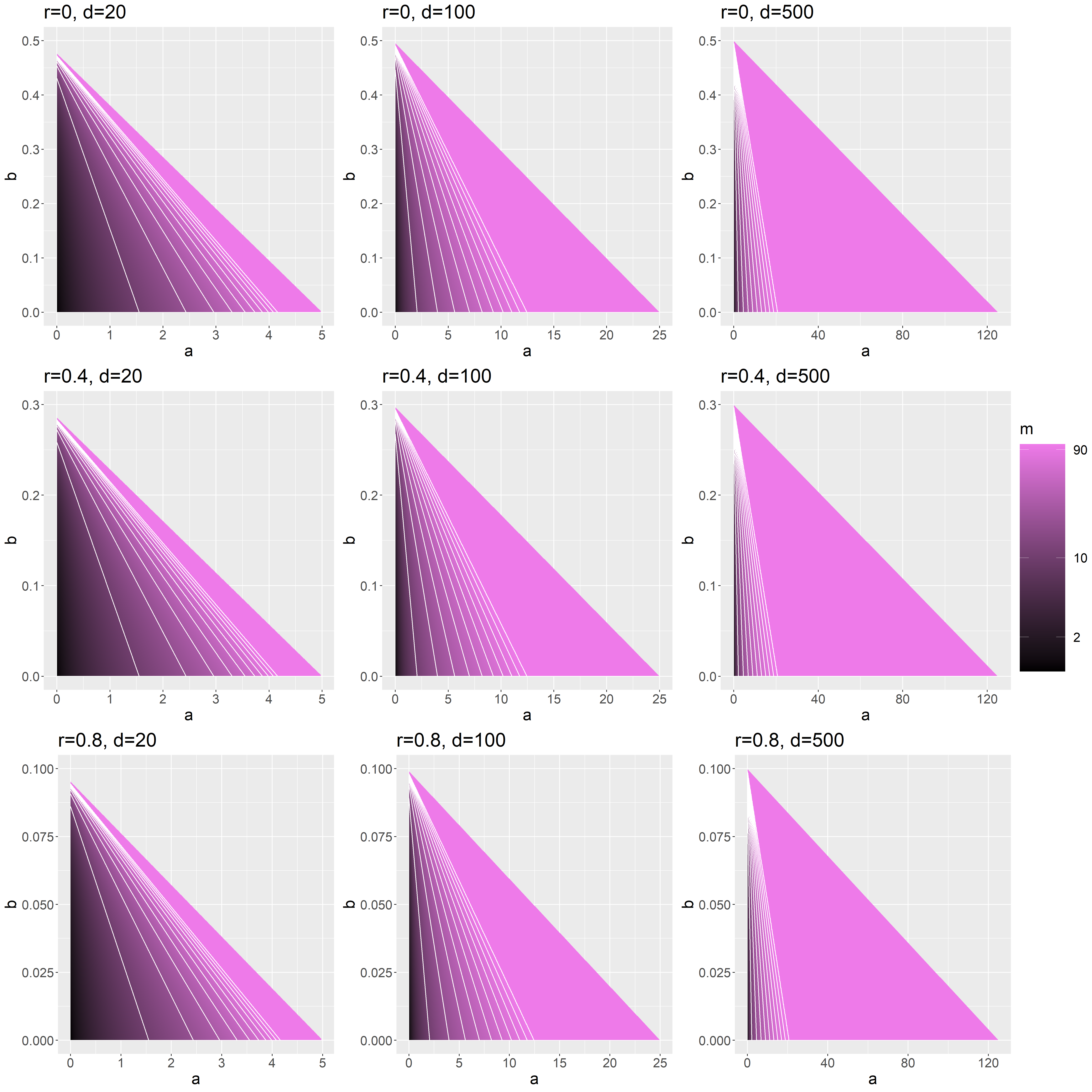
Figure 2: Required moments $m$ implied by eq. C.5. Contours mark intervals of 10 moments, and values above $m=100$ are truncated to 100. Non-shaded areas indicate infeasible regions.

C.4 Additional notes on Examples 5 and 6

We start with a lemma on useful properties of the matrix pseudo-norm induced by the $\left\lVert\cdot\right\rVert_{r}$ pseudo-norm. Its proof is omitted, but available upon request. We then provide further details on Examples 5 and 6.

Lemma C.1.

For matrices $\boldsymbol{A},\boldsymbol{B}\in\mathds{R}^{n\times m}$ with column vectors $\boldsymbol{a}_{j}$ and $\boldsymbol{b}_{j}$, define the induced matrix pseudo-norm $\left\lVert\boldsymbol{A}\right\rVert_{r}=\max\limits_{\boldsymbol{x}\neq\boldsymbol{0}}\frac{\left\lVert\boldsymbol{A}\boldsymbol{x}\right\rVert_{r}}{\left\lVert\boldsymbol{x}\right\rVert_{r}}=\max\limits_{\left\lVert\boldsymbol{x}\right\rVert_{r}=1}\left\lVert\boldsymbol{A}\boldsymbol{x}\right\rVert_{r}$, where for a vector $\boldsymbol{x}$ the pseudo-norm $\left\lVert\boldsymbol{x}\right\rVert_{r}=\left(\sum_{j}\left\lvert x_{j}\right\rvert^{r}\right)^{1/r}$. For $0<r<1$, the following hold

1. $\left\lVert cA\right\rVert_{r}=\left\lvert c\right\rvert\left\lVert A\right\rVert_{r}$,

2. $\left\lVert\boldsymbol{A}\right\rVert_{r}=\max_{j}\left\lVert\boldsymbol{a}_{j}\right\rVert_{r}$,

3. $\left\lVert\boldsymbol{A}\boldsymbol{B}\right\rVert_{r}\leq\left\lVert\boldsymbol{A}\right\rVert_{r}\left\lVert\boldsymbol{B}\right\rVert_{r}$,

4. $\left\lVert\boldsymbol{A}+\boldsymbol{B}\right\rVert_{r}^{r}\leq\left\lVert\boldsymbol{A}\right\rVert_{r}^{r}+\left\lVert\boldsymbol{B}\right\rVert_{r}^{r}$.

5. $m^{1/2-1/r}\left\lVert\boldsymbol{A}\right\rVert_{2}\leq\left\lVert\boldsymbol{A}\right\rVert_{r}\leq n^{1/r-1/2}\left\lVert\boldsymbol{A}\right\rVert_{2}$

For $r=0$, the induced matrix pseudo-norm $\left\lVert\boldsymbol{A}\right\rVert_{0}=\max\limits_{\boldsymbol{x}\neq\boldsymbol{0}}\frac{\left\lVert\boldsymbol{A}\boldsymbol{x}\right\rVert_{0}}{\left\lVert\boldsymbol{x}\right\rVert_{0}}$, with $\left\lVert\boldsymbol{x}\right\rVert_{0}=\sum_{j}\mathds{1}_{\{\left\lvert x_{j}\right\rvert>0\}}$. The above properties also hold for this norm, except property (5), and (1), which is replaced by

1. $\left\lVert c\boldsymbol{A}\right\rVert_{0}=\left\lVert\boldsymbol{A}\right\rVert_{0}$, for $c\neq 0$.

C.4.1 Example 5: Sparse factor model

Recall the factor model

$$\begin{split}y_{t}&=\boldsymbol{\beta^{0}}^{\prime}\boldsymbol{x}_{t}+u_{t},\ u_{t}\sim IID(0,1)\\ \boldsymbol{x}_{t}&=\underset{N\times k}{\boldsymbol{\Lambda}}\underset{k\times 1}{\boldsymbol{f}_{t}}+\boldsymbol{\nu}_{t},\ \boldsymbol{\nu}_{t}\sim IID(\boldsymbol{0},\boldsymbol{\Sigma}_{\boldsymbol{\nu}}),\qquad\boldsymbol{f}_{t}\sim IID(\boldsymbol{0},\boldsymbol{\Sigma}_{\boldsymbol{f}}),\end{split}$$

where $\boldsymbol{\Lambda}$ has bounded elements, $\boldsymbol{\Sigma}_{\boldsymbol{f}}$ and $\boldsymbol{\Sigma}_{\boldsymbol{\nu}}$ are positive definite with bounded eigenvalues, and $\boldsymbol{\nu}_{t}$ and $\boldsymbol{f}_{t}$ uncorrelated. We make the following assumptions on the factor loadings:

$$C_{1}N^{a}\leq\lambda_{\min}(\boldsymbol{\Lambda}^{\prime}\boldsymbol{\Lambda})\leq\lambda_{\max}(\boldsymbol{\Lambda}^{\prime}\boldsymbol{\Lambda})\leq C_{2}N^{b},\qquad 0<a\leq b\leq 1.$$ (C.6)

These assumptions imply that the $k$ largest eigenvalues of $\boldsymbol{\Sigma}=\boldsymbol{\Lambda}\boldsymbol{\Sigma}_{\boldsymbol{f}}\boldsymbol{\Lambda}^{\prime}+\boldsymbol{\Sigma}_{\boldsymbol{\nu}}$ diverge at rates between $N^{a}$ and $N^{b}$, while the remaining $N-k+1$ eigenvalues do not diverge. This holds as we can bound the largest eigenvalue $\lambda_{\max}(\boldsymbol{\Sigma})$ from above by

$$\begin{split}\lambda_{\max}(\boldsymbol{\Sigma})&\leq\lambda_{\max}(\boldsymbol{\Lambda}\boldsymbol{\Sigma}_{\boldsymbol{f}}\boldsymbol{\Lambda}^{\prime})+\lambda_{\max}(\boldsymbol{\Sigma}_{\boldsymbol{\nu}})\leq\lambda_{\max}(\boldsymbol{\Sigma}_{\boldsymbol{f}})\lambda_{\max}(\boldsymbol{\Lambda}^{\prime}\boldsymbol{\Lambda})+\lambda_{\max}(\boldsymbol{\Sigma}_{\boldsymbol{\nu}})\leq C_{1}N^{b}+C_{2}.\end{split}$$

Similarly, we can bound bound the $k$-th largest eigenvalue $\lambda_{k}(\boldsymbol{\Sigma})$ using Weyl’s inequality and the min-max theorem from below by

$$\begin{split}\lambda_{k}(\boldsymbol{\Sigma})&\geq\lambda_{k}(\boldsymbol{\Lambda}\boldsymbol{\Sigma}_{\boldsymbol{f}}\boldsymbol{\Lambda}^{\prime})+\lambda_{\min}(\boldsymbol{\Sigma}_{\boldsymbol{\nu}})=\max_{\mathcal{U}}\left\{\left.\min_{\boldsymbol{x}\in\mathcal{U}\setminus\boldsymbol{0}}\frac{\boldsymbol{x}^{\prime}\boldsymbol{\Lambda}\boldsymbol{\Sigma}_{\boldsymbol{f}}\boldsymbol{\Lambda}^{\prime}\boldsymbol{x}}{\boldsymbol{x}^{\prime}\boldsymbol{x}}\right|\dim(\mathcal{U})=N-k+1\right\}+\lambda_{\min}(\boldsymbol{\Sigma}_{\boldsymbol{\nu}})\\ &\geq\lambda_{\min}(\boldsymbol{\Sigma}_{\boldsymbol{f}})\max_{\mathcal{U}}\left\{\left.\min_{\boldsymbol{x}\in\mathcal{U}\setminus\boldsymbol{0}}\frac{\boldsymbol{x}^{\prime}\boldsymbol{\Lambda}\boldsymbol{\Lambda}^{\prime}\boldsymbol{x}}{\boldsymbol{x}^{\prime}\boldsymbol{x}}\right|\dim(\mathcal{U})=N-k+1\right\}+\lambda_{\min}(\boldsymbol{\Sigma}_{\boldsymbol{\nu}})\\ &=\lambda_{\min}(\boldsymbol{\Sigma}_{\boldsymbol{f}})\lambda_{k}(\boldsymbol{\Lambda}\boldsymbol{\Lambda}^{\prime})+\lambda_{\min}(\boldsymbol{\Sigma}_{\boldsymbol{\nu}})=\lambda_{\min}(\boldsymbol{\Sigma}_{\boldsymbol{f}})\lambda_{\min}(\boldsymbol{\Lambda}\boldsymbol{\Lambda}^{\prime})+\lambda_{\min}(\boldsymbol{\Sigma}_{\boldsymbol{\nu}})\geq C_{1}N^{a}+C_{2},\end{split}$$

where we used that $\lambda_{k}(\boldsymbol{\Lambda}\boldsymbol{\Lambda}^{\prime})=\lambda_{k}(\boldsymbol{\Lambda}^{\prime}\boldsymbol{\Lambda})=\lambda_{\min}(\boldsymbol{\Lambda}^{\prime}\boldsymbol{\Lambda})$.

Therefore, this assumption generates a weak factor model if $b<1$, while if $b=1$ but $a<1$ some factors, but not all, are weak; see e.g. Uematsu and Yamagata (2022a, b) and the references therein. If $a=b=1$ we have the standard strong factor model with dense loadings.

Sparse factor loadings satisfy these assumptions. In particular, from Lemma C.1(5) we find that $\lambda_{\max}(\boldsymbol{\Lambda}^{\prime}\boldsymbol{\Lambda})=\left\lVert\boldsymbol{\Lambda}\right\rVert_{2}^{2}\leq k^{2/r-1}\left\lVert\boldsymbol{\Lambda}\right\rVert_{r}^{2}$; thus, with a fixed number $k$ of factors, the sparsity of $\boldsymbol{\Lambda}$ provides an upper bound for the strength of divergence of the largest eigenvalues. Sparse factor models may provide accurate descriptions of various economic and financial datasets. For example, Uematsu and Yamagata (2022b) find strong evidence of sparse factor loadings in the FRED-MD macroeconomic dataset (McCracken and Ng, 2016), as well as of firm-level excess returns of the S&P500 beyond the market return factor. Freyaldenhoven (2021) uses sparsity in the loadings to identify the factors, motivating the sparsity empirically through the presence of “local” factors in economic and financial data. Further empirical evidence for sparse factor models is reviewed in Uematsu and Yamagata (2022a).

We now derive the sparsity bound of Example 5. We bound $\left\lVert\boldsymbol{\gamma}_{j}^{0}\right\rVert_{r}^{r}$ based on the fact that $\boldsymbol{\Theta}=\boldsymbol{\Upsilon}^{-2}\boldsymbol{\Gamma}$, where $\boldsymbol{\Upsilon}^{-2}=\text{diag}(1/\tau_{1}^{2},\dots,1/\tau_{N}^{2})$, and

$${\boldsymbol{\Gamma}}:=\begin{bmatrix}1&-{\gamma}_{1,2}&\dots&-{\gamma}_{1,N}\\ -{\gamma}_{2,1}&1&\dots&-{\gamma}_{2,N}\\ \vdots&\vdots&\ddots&\vdots\\ -{\gamma}_{N,1}&-{\gamma}_{N,2}&\dots&1\end{bmatrix}.$$

This result follows from the definition of $\boldsymbol{\gamma}_{j}^{0}$ as linear projection coefficients, and the block matrix inverse identity for $\boldsymbol{\Theta}$. Then

$$\begin{split}\max_{j}\left\lVert\boldsymbol{\gamma}_{j}^{0}\right\rVert^{r}_{r}\leq&1+\max_{j}\left\lVert\boldsymbol{\gamma}_{j}^{0}\right\rVert^{r}_{r}=\max_{j}\left\lVert(1,\boldsymbol{\gamma}_{j}^{0\prime})^{\prime}\right\rVert_{r}^{r}=\max_{j}\left\lVert(1,-\boldsymbol{\gamma}_{j}^{0\prime})^{\prime}\right\rVert_{r}^{r}=\left\lVert\boldsymbol{\Gamma}\right\rVert_{r}^{r}\\ =&\left\lVert(\boldsymbol{\Upsilon}^{-2})^{-1}\boldsymbol{\Theta}\right\rVert_{r}^{r}\leq\left\lVert(\boldsymbol{\Upsilon}^{-2})^{-1}\right\rVert_{r}^{r}\left\lVert\boldsymbol{\Theta}\right\rVert_{r}^{r}\leq\max_{j}\tau_{j}^{2r}\left\lVert\boldsymbol{\Theta}\right\rVert_{r}^{r}\leq C\left\lVert\boldsymbol{\Theta}\right\rVert_{r}^{r},\end{split}$$

where $\max_{j}\tau_{j}^{2r}\leq C$ follows from (B.1) Note that when $r=0$, these steps follow similarly, noting that $\left\lVert(\boldsymbol{\Upsilon}^{-2})^{-1}\right\rVert_{0}=1$, and therefore $C=1$.

By the Woodbury matrix identity

$$\begin{split}\boldsymbol{\Theta}&=\boldsymbol{\Sigma}_{\boldsymbol{\nu}}^{-1}-\boldsymbol{\Sigma}_{\boldsymbol{\nu}}^{-1}\boldsymbol{\Lambda}/N^{a}\left(\boldsymbol{\Sigma}_{\boldsymbol{f}}^{-1}/N^{a}+\boldsymbol{\Lambda}^{\prime}\boldsymbol{\Sigma}_{\boldsymbol{\nu}}^{-1}\boldsymbol{\Lambda}/N^{a}\right)^{-1}\boldsymbol{\Lambda}^{\prime}\boldsymbol{\Sigma}_{\boldsymbol{\nu}}^{-1}.\end{split}$$

Then

$$\begin{split}\left\lVert\boldsymbol{\Theta}\right\rVert_{r}^{r}&\leq\left\lVert\boldsymbol{\Sigma}_{\boldsymbol{\nu}}^{-1}\right\rVert_{r}^{r}+\left\lVert\boldsymbol{\Sigma}_{\boldsymbol{\nu}}^{-1}\right\rVert_{r}^{r}\left\lVert\boldsymbol{\Lambda}/N^{a}\right\rVert_{r}^{r}\left\lVert\left(\boldsymbol{\Sigma}_{\boldsymbol{f}}^{-1}/N^{a}+\boldsymbol{\Lambda}^{\prime}\boldsymbol{\Sigma}_{\boldsymbol{\nu}}^{-1}\boldsymbol{\Lambda}/N^{a}\right)^{-1}\right\rVert_{r}^{r}\left\lVert\boldsymbol{\Lambda}^{\prime}\right\rVert_{r}^{r}\left\lVert\boldsymbol{\Sigma}_{\boldsymbol{\nu}}^{-1}\right\rVert_{r}^{r}.\end{split}$$

As for positive semidefinite symmetric matrices $\boldsymbol{A}$ and $\boldsymbol{B}$ we have that

$$\left\lVert(\boldsymbol{A}+\boldsymbol{B})^{-1}\right\rVert_{2}\leq\frac{1}{\lambda_{\min}(\boldsymbol{A}+\boldsymbol{B})}\leq\frac{1}{\lambda_{\min}(\boldsymbol{A})+\lambda_{\min}(\boldsymbol{B})}\leq\frac{1}{\lambda_{\min}(\boldsymbol{B})},$$

it follows that

$$\begin{split}\left\lVert\left(\boldsymbol{\Sigma}_{\boldsymbol{f}}^{-1}/N^{a}+\boldsymbol{\Lambda}^{\prime}\boldsymbol{\Sigma}_{\boldsymbol{\nu}}^{-1}\boldsymbol{\Lambda}/N^{a}\right)^{-1}\right\rVert_{2}\leq\frac{1}{\lambda_{\min}\left(\boldsymbol{\Lambda}^{\prime}\boldsymbol{\Sigma}_{\boldsymbol{\nu}}^{-1}\boldsymbol{\Lambda}/N^{a}\right)}\leq\frac{1}{\lambda_{\min}(\boldsymbol{\Sigma}_{\boldsymbol{\nu}}^{-1})\lambda_{\min}\left(\boldsymbol{\Lambda}^{\prime}\boldsymbol{\Lambda}/N^{a}\right)}.\end{split}$$

As $\lambda_{\min}(\boldsymbol{\Sigma}_{\boldsymbol{\nu}}^{-1})=1/\lambda_{\max}(\boldsymbol{\Sigma}_{\boldsymbol{\nu}})\geq 1/C$, it follows from our assumptions that $\lambda_{\min}\left(\boldsymbol{\Lambda}^{\prime}\boldsymbol{\Lambda}/N^{a}\right)\geq C$ and therefore $\left\lVert\left(\boldsymbol{\Sigma}_{\boldsymbol{f}}^{-1}/N+\boldsymbol{\Lambda}^{\prime}\boldsymbol{\Sigma}_{\boldsymbol{\nu}}^{-1}\boldsymbol{\Lambda}/N\right)^{-1}\right\rVert_{2}\leq C$. It then also follows from Lemma C.1(5) that $\left\lVert\left(\boldsymbol{\Sigma}_{\boldsymbol{f}}^{-1}/N^{a}+\boldsymbol{\Lambda}^{\prime}\boldsymbol{\Sigma}_{\boldsymbol{\nu}}^{-1}\boldsymbol{\Lambda}/N^{a}\right)^{-1}\right\rVert_{r}^{r}\leq Ck^{1-r/2}$ and

$$\begin{split}\left\lVert\boldsymbol{\Theta}\right\rVert_{r}^{r}&\leq\left\lVert\boldsymbol{\Sigma}_{\boldsymbol{\nu}}^{-1}\right\rVert_{r}^{r}+Ck^{1-r/2}\left\lVert\boldsymbol{\Sigma}_{\boldsymbol{\nu}}^{-1}\right\rVert_{r}^{r}\left\lVert\boldsymbol{\Lambda}/N^{a}\right\rVert_{r}^{r}\left\lVert\boldsymbol{\Lambda}^{\prime}\right\rVert_{r}^{r}\left\lVert\boldsymbol{\Sigma}_{\boldsymbol{\nu}}^{-1}\right\rVert_{r}^{r}.\end{split}$$ (C.7)

With $\left\lVert\boldsymbol{\Lambda}^{\prime}\right\rVert_{r}^{r}\leq Ck$, we then find the bound

$$\begin{split}\left\lVert\boldsymbol{\Theta}\right\rVert_{r}^{r}&\leq\left\lVert\boldsymbol{\Sigma}_{\boldsymbol{\nu}}^{-1}\right\rVert_{r}^{r}+Ck^{2-r/2}N^{-ra}\left\lVert\boldsymbol{\Sigma}_{\boldsymbol{\nu}}^{-1}\right\rVert_{r}^{2r}\left\lVert\boldsymbol{\Lambda}\right\rVert_{r}^{r}.\end{split}$$

We provide two examples of $\boldsymbol{\Sigma}_{\boldsymbol{\nu}}$ such that $\boldsymbol{\Sigma}_{\boldsymbol{\nu}}^{-1}$ is sparse. For block diagonal structures, this follows trivially, since the inverse maintains the same block diagonal structure. For a Toeplitz structure $\boldsymbol{\Sigma}_{\boldsymbol{\nu},i,j}=\rho^{\left\lvert i-j\right\rvert}$, by Section 8.8.4 of Gentle (2007),

$$\boldsymbol{\Sigma}_{\boldsymbol{\nu}}^{-1}=\frac{1}{1-\rho^{2}}\begin{bmatrix}1&-\rho&0&\dots&0\\ -\rho&1+\rho^{2}&-\rho&\dots&0\\ 0&-\rho&1+\rho^{2}&\dots&0\\ \vdots&\vdots&\vdots&\vdots&\vdots\\ 0&0&0&\dots&1\end{bmatrix},$$

and we can bound

$$\left\lVert\boldsymbol{\Sigma}_{\boldsymbol{\nu}}^{-1}\right\rVert_{r}^{r}=\max\limits_{j}\left\lVert\boldsymbol{\Sigma}_{\boldsymbol{\nu},\cdot,j}^{-1}\right\rVert_{r}^{r}=\left\lVert\boldsymbol{\Sigma}^{-1}_{\boldsymbol{\nu},\cdot,\left\lceil{N/2}\right\rceil}\right\rVert_{r}^{r}=\frac{\left\lvert 1+\rho^{2}\right\rvert^{r}+2\left\lvert\rho\right\rvert^{r}}{\left\lvert 1-\rho^{2}\right\rvert^{r}}\leq C,$$

or simply $\max\limits_{j}\left\lVert\boldsymbol{\Sigma}_{\boldsymbol{\nu},\cdot,j}^{-1}\right\rVert_{0}=3$ for $r=0$.

Note that a (potentially weak) factor model without sparse loadings does not yield a sufficiently sparse matrix $\boldsymbol{\Theta}$ for all values of $r$. In eq. C.7 we may try to bound $\left\lVert\boldsymbol{\Lambda}\right\rVert_{r}^{r}$ directly using Lemma C.1(5) to bound $\left\lVert\boldsymbol{\Lambda}/N^{a}\right\rVert_{r}^{r}\leq N^{1+(b-2a-1)r/2}\left[\lambda_{\max}(\boldsymbol{\Lambda}^{\prime}\boldsymbol{\Lambda}/N^{b})\right]^{r/2}$, such that $\left\lVert\boldsymbol{\Theta}\right\rVert_{r}^{r}\leq\left\lVert\boldsymbol{\Sigma}_{\boldsymbol{\nu}}^{-1}\right\rVert_{r}^{r}\left(1+Ck^{2-r/2}N^{1+(b-2a-1)r/2}\right)$. This is not a tight enough bound to guarantee sparsity of $\boldsymbol{\Theta}$. To illustrate, for the standard dense factor model with $a=b=1$ and $k$ fixed, we get $\left\lVert\boldsymbol{\Theta}\right\rVert_{r}^{r}\leq CN^{1-r}$. Weaker divergence of the eigenvalues even increases the power of $N$.

C.4.2 Example 6: Sparse VAR(1)

Recall the sparse VAR(1) model

$$\boldsymbol{z}_{t}=\boldsymbol{\Phi}\boldsymbol{z}_{t-1}+\boldsymbol{u}_{t},\ \mathbb{E}\boldsymbol{u}_{t}\boldsymbol{u}_{t}^{\prime}:=\boldsymbol{\Omega},\ \mathbb{E}\boldsymbol{u}_{t}\boldsymbol{u}_{t-l}^{\prime}=\boldsymbol{0},\ \forall l\neq 0,$$

with our regression of interest being $y_{t}=\boldsymbol{\phi}_{1}\boldsymbol{z}_{t-1}+u_{1,t}$. For Example 6(a) with a symmetric block-diagonal coefficient matrix $\boldsymbol{\Phi}$ and the error covariance matrix $\boldsymbol{\Omega}$ being the identity, we can simplify $\boldsymbol{\Sigma}=\sum\limits_{q=0}^{\infty}\boldsymbol{\Phi}^{q}\boldsymbol{\Omega}\boldsymbol{\Phi}^{\prime q}=\sum\limits_{q=0}^{\infty}\boldsymbol{\Phi}^{2q}=\left(\boldsymbol{I}-\boldsymbol{\Phi}^{2}\right)^{-1}$, where $\boldsymbol{\Phi}^{0}=\boldsymbol{\Phi}^{\prime 0}=\boldsymbol{I}$, and $\boldsymbol{\Theta}=\boldsymbol{\Sigma}^{-1}=\boldsymbol{I}-\boldsymbol{\Phi}^{2}$. Note that $\boldsymbol{I}-\boldsymbol{A}$ is invertible iff 1 is not an eigenvalue of $\boldsymbol{A}$. Since the eigenvalues of $\boldsymbol{\Phi}^{2}$ are between (and not including) 0 and 1, $\boldsymbol{\Sigma}$ exists. $\boldsymbol{I}-\boldsymbol{\Phi}^{2}$ inherits the block diagonal structure of $\boldsymbol{\Phi}$, so we may bound $\max\limits_{j}\left\lVert\boldsymbol{\gamma}_{j}^{0}\right\rVert_{r}^{r}\leq C\left\lVert\boldsymbol{\Theta}\right\rVert_{r}^{r}\leq Cb$.

This result can be extended to the case where $\boldsymbol{\Omega}$ has the same block diagonal structure as the VAR coefficient matrix $\boldsymbol{\Phi}$. While the simplified expression for $\boldsymbol{\Sigma}$ provided above no longer holds, both $\boldsymbol{\Sigma}$ and $\boldsymbol{\Sigma}^{-1}$ remain block diagonal when $\boldsymbol{\Omega}$ and $\boldsymbol{\Phi}$ share the same block structure. As a result, the nonzero structure of $\boldsymbol{\gamma}_{j}^{0}$ remains unaltered.

For Example 6(b) with a diagonal $\boldsymbol{\Phi}$ and Toeplitz $\boldsymbol{\Omega}$, we can simplify $\boldsymbol{\Sigma}=\sum\limits_{q=0}^{\infty}\boldsymbol{\Phi}^{q}\boldsymbol{\Omega}\boldsymbol{\Phi}^{\prime q}=\sum\limits_{q=0}^{\infty}\phi^{2q}\boldsymbol{\Omega}=\frac{1}{1-\phi^{2}}\boldsymbol{\Omega}$ and by similar arguments to section C.4.1,

$$\boldsymbol{\Theta}=\frac{1-\phi^{2}}{1-\rho^{2}}\begin{bmatrix}1&-\rho&0&\dots&0\\ -\rho&1+\rho^{2}&-\rho&\dots&0\\ 0&-\rho&1+\rho^{2}&\dots&0\\ \vdots&\vdots&\vdots&\vdots&\vdots\\ 0&0&0&\dots&1\end{bmatrix}$$

. The precision matrix is clearly sparse in this case, and $\max\limits_{j}\left\lVert\boldsymbol{\gamma}_{j}^{0}\right\rVert_{r}^{r}\leq C\left\lVert\boldsymbol{\Theta}\right\rVert_{r}^{r}\leq C$.

Finally, we numerically investigated the extension where the VAR coefficient matrix also has a Toeplitz structure, namely $\Phi_{i,j}=0.4^{1+\left\lvert i-j\right\rvert}$. We vary the sample size between $N=10$ and $N=1000$ and display the boundedness in $r$-norm of the parameter vector in the nodewise regressions in Figure 3 for different values of $r$. We use a log-scale since this sparsity grows by orders of magnitude for decreasing $r$.

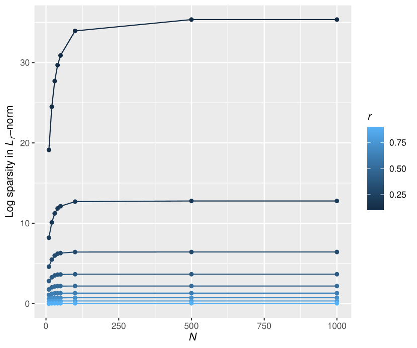
Figure 3: Example 6(b): We display $\ln\left(\max\limits_{j}\left\lVert\boldsymbol{\gamma}_{j}^{0}\right\rVert_{r}^{r}\right)$ for $N$ between 10 and 1000, and $r$ between 0.1 and 0.9.

C.5 Algorithmic details for choosing the lasso tuning parameter

At $k=0$, initialize $\lambda^{(0)}\leftarrow\left\lVert\boldsymbol{X}^{\prime}\boldsymbol{y}\right\rVert_{\infty}/T$ and $\hat{\boldsymbol{u}}^{(0)}\leftarrow\boldsymbol{y}-\frac{1}{T}\sum_{t=1}^{T}y_{t}$;

while $1\leq k\leq K$ do

       Obtain the estimated long-run covariance matrix $\hat{\boldsymbol{\Omega}}^{(k)}$ as in (9), with $\hat{\boldsymbol{\Xi}}(l)=\frac{1}{T-l}\sum\limits_{t=l+1}^{T}\boldsymbol{x}_{t}\hat{u}^{(k-1)}_{t}\hat{u}^{(k-1)}_{t-l}\boldsymbol{x}_{t-l}^{\prime}$;

       while $1\leq b\leq B$ do

             Draw $\hat{\boldsymbol{g}}^{(b)}$ from $N\left(\boldsymbol{0},\hat{\boldsymbol{\Omega}}^{(k)}\right)$;

             $m_{b}\leftarrow\left\lVert\hat{\boldsymbol{g}}^{(b)}\right\rVert_{\infty}$;

            

      $\lambda^{(k)}\leftarrow c\frac{1}{\sqrt{T}}q_{(1-\alpha)}$, where $q_{(1-\alpha)}$ is the $(1-\alpha)$-quantile of $m_{1},\ldots,m_{B}$;

       if $\left\lvert\lambda^{(k)}-\lambda^{(k-1)}\right\rvert/\lambda^{(k-1)}<\epsilon$ then

            $\lambda\leftarrow\lambda^{(k)}$;

             break;

            

      else

             Estimate $\hat{\boldsymbol{\beta}}^{(k)}$ with the lasso using $\lambda^{(k)}$ as the tuning parameter;

             $\hat{\boldsymbol{u}}^{(k)}\leftarrow\boldsymbol{y}-\boldsymbol{X}\hat{\boldsymbol{\beta}}^{(k)}$;

            

      

$\lambda\leftarrow\lambda^{(K)}$;

Algorithm 1 Plug-in choice of $\lambda$

We set $K=15$, $\epsilon=0.01$, $B=1000$, $\alpha=0.05$, and $c=0.8$ throughout the simulation study.

C.6 Additional simulation details

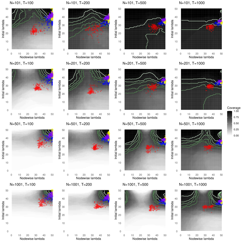
Figure 4: Model A, $\rho$ heat map coverage: Contours mark the coverage thresholds at 5% intervals, from 75% to the nominal 95%, from dark green to white respectively. Units on the axes are not proportional to the $\lambda$-value but rather its position in the grid. The value of $\lambda$ is $(10T)^{-1}$ at 0, and increases exponentially to a value that sets all parameters to zero at 50. Plots are based on 100 replications, with colored dots representing combinations of $\lambda$’s selected by PI (purple), AIC (red), BIC (blue), EBIC (yellow).

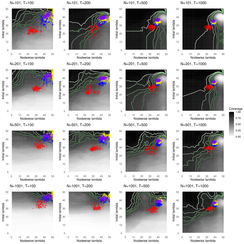
Figure 5: Model A, $\beta_{1}$ heat map coverage: Contours mark the coverage thresholds at 5% intervals, from 75% to the nominal 95%, from dark green to white respectively. Units on the axes are not proportional to the $\lambda$-value but rather its position in the grid. The value of $\lambda$ is $(10T)^{-1}$ at 0, and increases exponentially to a value that sets all parameters to zero at 50. Plots are based on 100 replications, with colored dots representing combinations of $\lambda$’s selected by PI (purple), AIC (red), BIC (blue), EBIC (yellow).

Figure 6: Model B, $\rho$ heat map coverage: Contours mark the coverage thresholds at 5% intervals, from 75% to the nominal 95%, from dark green to white respectively. Units on the axes are not proportional to the $\lambda$-value but rather its position in the grid. The value of $\lambda$ is $(10T)^{-1}$ at 0, and increases exponentially to a value that sets all parameters to zero at 50. Plots are based on 100 replications, with colored dots representing combinations of $\lambda$’s selected by PI (purple), AIC (red), BIC (blue), EBIC (yellow).

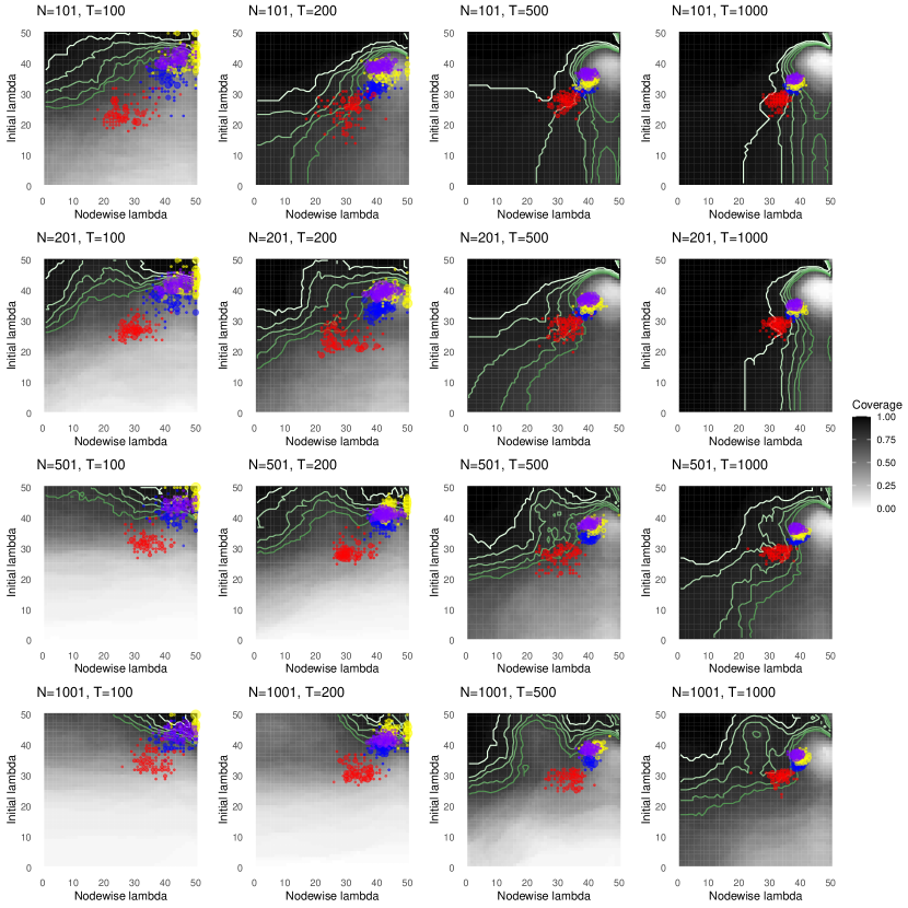
Figure 7: Model B, $\beta_{1}$ heat map coverage: Contours mark the coverage thresholds at 5% intervals, from 75% to the nominal 95%, from dark green to white respectively. Units on the axes are not proportional to the $\lambda$-value but rather its position in the grid. The value of $\lambda$ is $(10T)^{-1}$ at 0, and increases exponentially to a value that sets all parameters to zero at 50. Plots are based on 100 replications, with colored dots representing combinations of $\lambda$’s selected by PI (purple), AIC (red), BIC (blue), EBIC (yellow).

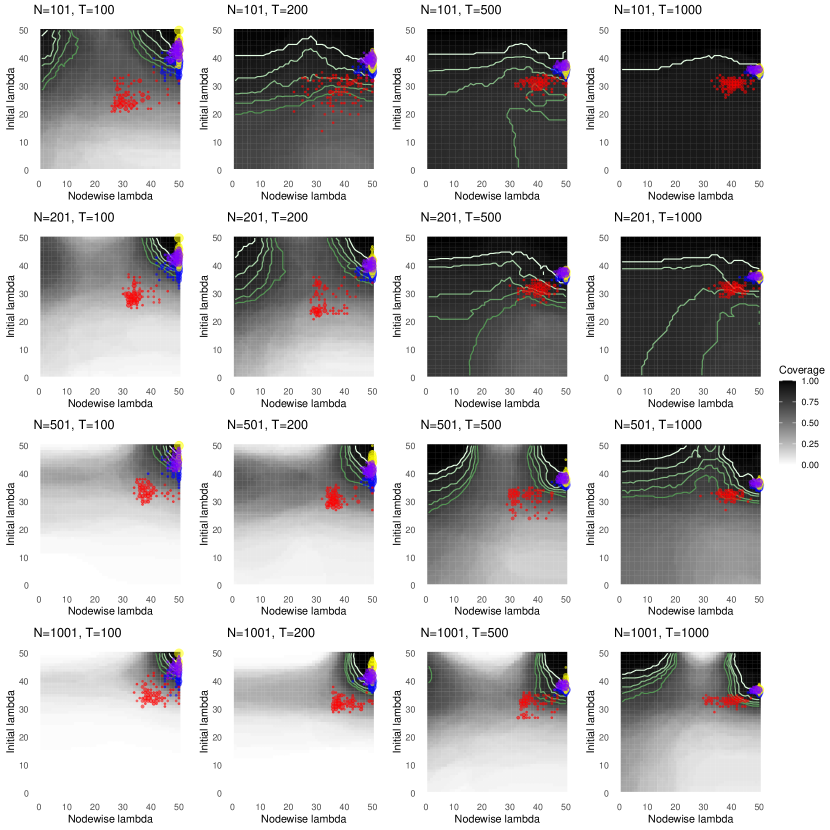
Figure 8: Model C, $\rho$ heat map coverage: Contours mark the coverage thresholds at 5% intervals, from 75% to the nominal 95%, from dark green to white respectively. Units on the axes are not proportional to the $\lambda$-value but rather its position in the grid. The value of $\lambda$ is $(10T)^{-1}$ at 0, and increases exponentially to a value that sets all parameters to zero at 50. Plots are based on 100 replications, with colored dots representing combinations of $\lambda$’s selected by PI (purple), AIC (red), BIC (blue), EBIC (yellow).

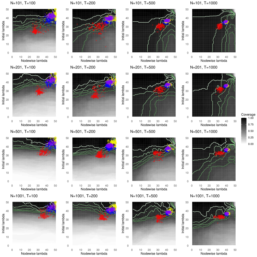
Figure 9: Model C, $\beta_{1}$ heat map coverage: Contours mark the coverage thresholds at 5% intervals, from 75% to the nominal 95%, from dark green to white respectively. Units on the axes are not proportional to the $\lambda$-value but rather its position in the grid. The value of $\lambda$ is $(10T)^{-1}$ at 0, and increases exponentially to a value that sets all parameters to zero at 50. Plots are based on 100 replications, with colored dots representing combinations of $\lambda$’s selected by PI (purple), AIC (red), BIC (blue), EBIC (yellow).

References

- Andrews (1984) Andrews, D. W. (1984). Non-strong mixing autoregressive processes. Journal of Applied Probability 21(4), 930–934.
- Andrews (1991) Andrews, D. W. (1991). Heteroskedasticity and autocorrelation consistent covariance matrix estimation. Econometrica 59, 817–858.
- Babii et al. (2021) Babii, A., E. Ghysels, and J. Striaukas (2021). High-dimensional Granger causality tests with an application to VIX and news. arXiv e-print 1912.06307.
- Bachoc et al. (2020) Bachoc, F., D. Preinerstorfer, and L. Steinberger (2020). Uniformly valid confidence intervals post-model-selection. Annals of Statistics 48(1), 440–463.
- Bai and Ng (2008) Bai, J. and S. Ng (2008). Large dimensional factor analysis. Foundations and Trends in Econometrics 3(2), 89–163.
- Basu and Michailidis (2015) Basu, S. and G. Michailidis (2015). Regularized estimation in sparse high-dimensional time series models. Annals of Statistics 43(4), 1535–1567.
- Belloni et al. (2012) Belloni, A., D. Chen, V. Chernozhukov, and C. Hansen (2012). Sparse models and methods for optimal instruments with an application to eminent domain. Econometrica 80(6), 2369–2429.
- Belloni et al. (2017) Belloni, A., V. Chernozhukov, I. Fernández-Val, and C. Hansen (2017). Program evaluation and causal inference with high-dimensional data. Econometrica 85(1), 233–298.
- Belloni et al. (2014) Belloni, A., V. Chernozhukov, and C. Hansen (2014). Inference on treatment effects after selection among high-dimensional controls. Review of Economic Studies 81(2), 608–650.
- Berk et al. (2013) Berk, R., L. Brown, A. Buja, K. Zhang, and L. Zhao (2013). Valid post-selection inference. Annals of Statistics 41(2), 802–837.
- Beutner et al. (2021) Beutner, E., A. Heinemann, and S. Smeekes (2021). A justification of conditional confidence intervals. Electronic Journal of Statistics 15(1), 2517–2565.
- Bickel et al. (2009) Bickel, P. J., Y. Ritov, and A. B. Tsybakov (2009). Simultaneous analysis of lasso and dantzig selector. Annals of Statistics 37(4), 1705–1732.
- Bühlmann (2006) Bühlmann, P. (2006). Boosting for high-dimensional linear models. Annals of Statistics 34(2), 559–583.
- Bühlmann and van De Geer (2011) Bühlmann, P. and S. van De Geer (2011). Statistics for High-Dimensional Data: Methods, Theory and Applications. Springer.
- Bunea et al. (2007) Bunea, F., A. Tsybakov, and M. Wegkamp (2007). Sparsity oracle inequalities for the Lasso. Electronic Journal of Statistics 1, 169–194.
- Casella and Berger (2002) Casella, G. and R. L. Berger (2002). Statistical Inference (2 ed.). Duxbury.
- Chang et al. (2021) Chang, J., X. Chen, and M. Wu (2021). Central limit theorems for high dimensional dependent data. arXiv e-print 2104.12929.
- Chen and Chen (2012) Chen, J. and Z. Chen (2012). Extended BIC for small-n-large-P sparse GLM. Statistica Sinica 22(2), 555–574.
- Chernozhukov et al. (2018) Chernozhukov, V., D. Chetverikov, M. Demirer, E. Duflo, C. Hansen, W. Newey, and J. Robins (2018). Double/debiased machine learning for treatment and structural parameters. Econometrics Journal 21(1), C1–C68.
- Chernozhukov et al. (2013) Chernozhukov, V., D. Chetverikov, and K. Kato (2013). Gaussian approximations and multiplier bootstrap for maxima of sums of high-dimensional random vectors. Annals of Statistics 41(6), 2786–2819.
- Chernozhukov et al. (2015) Chernozhukov, V., D. Chetverikov, and K. Kato (2015). Comparison and anti-concentration bounds for maxima of Gaussian random vectors. Probability Theory and Related Fields 162(1), 47–70.
- Chernozhukov et al. (2019) Chernozhukov, V., D. Chetverikov, and K. Kato (2019). Inference on causal and structural parameters using many moment inequalities. The Review of Economic Studies 86(5), 1867–1900.
- Chernozhukov et al. (2015) Chernozhukov, V., C. Hansen, and M. Spindler (2015). Valid post-selection and post-regularization inference: an elementary, general approach. Annual Review of Economics 7, 649–688.
- Chernozhukov et al. (2021) Chernozhukov, V., W. K. Härdle, C. Huang, and W. Wang (2021). LASSO-driven inference in time and space. The Annals of Statistics 49(3), 1702–1735.
- Davidson (2002a) Davidson, J. (2002a). Establishing conditions for the functional central limit theorem in nonlinear and semiparametric time series processes. Journal of Econometrics 106(2), 243–269.
- Davidson (2002b) Davidson, J. (2002b). Stochastic Limit Theory (2nd ed.). Oxford: Oxford University Press.
- De Mol et al. (2008) De Mol, C., D. Giannone, and L. Reichlin (2008). Forecasting using a large number of predictors: Is bayesian shrinkage a valid alternative to principal components? Journal of Econometrics 146(2), 318–328.
- Deshpande et al. (2020) Deshpande, Y., A. Javanmard, and M. Mehrabi (2020). Online debiasing for adaptively collected high-dimensional data with applications to time series analysis. arXiv e-print 1911.01040.
- Dezeure et al. (2017) Dezeure, R., P. Bühlmann, and C.-H. Zhang (2017). High-dimensional simultaneous inference with the bootstrap. Test 26(4), 685–719.
- Fithian et al. (2015) Fithian, W., D. Sun, and J. Taylor (2015). Optimal inference after model selection. arXiv e-print 1410.2597.
- Francq and Zakoïan (2010) Francq, C. and J.-M. Zakoïan (2010). GARCH Models: Structure, Statistical Inference and Financial Applications. Wiley.
- Freyaldenhoven (2021) Freyaldenhoven, S. (2021). Identification through sparsity in factor models: The -rotation criterion. Working Paper WP 20-25/R, Federal Reserve Bank of Philadelphia.
- Friedman et al. (2010) Friedman, J. H., T. Hastie, and R. Tibshirani (2010). Regularization paths for generalized linear models via coordinate descent. Journal of Statistical Software 33(1), 1–22.
- Gentle (2007) Gentle, J. E. (2007). Matrix Algebra. Springer.
- Gonçalves and Vogelsang (2011) Gonçalves, S. and T. J. Vogelsang (2011). Block bootstrap HAC robust tests: the sophistication of the naive bootstrap. Econometric Theory 27(4), 745–791.
- Greenshtein and Ritov (2004) Greenshtein, E. and Y. Ritov (2004). Persistence in high-dimensional linear predictor selection and the virtue of overparametrization. Bernoulli 10(6), 971–988.
- Hansen (1991a) Hansen, B. E. (1991a). GARCH(1, 1) processes are near epoch dependent. Economics Letters 36(2), 181–186.
- Hansen (1991b) Hansen, B. E. (1991b). Strong laws for dependent heterogeneous processes. Econometric Theory 7(2), 213–221.
- Hastie et al. (2015) Hastie, T., R. Tibshirani, and M. Wainwright (2015). Statistical Learning with Sparsity: The Lasso and Generalizations. Chapman and Hall/CRC.
- Hecq et al. (2019) Hecq, A., L. Margaritella, and S. Smeekes (2019). Granger causality testing in high-dimensional VARs: a post-double-selection procedure. arXiv e-print 1902.10991.
- Hesterberg et al. (2008) Hesterberg, T., N. H. Choi, L. Meier, and C. Fraley (2008). Least angle and penalized regression: A review. Statistics Surveys 2, 61–93.
- Hsu et al. (2008) Hsu, N.-J., H.-L. Hung, and Y.-M. Chang (2008). Subset selection for vector autoregressive processes using lasso. Computational Statistics & Data Analysis 52(7), 3645–3657.
- Huang et al. (2008) Huang, J., S. Ma, and C.-H. Zhang (2008). Adaptive lasso for sparse high-dimensional regression models. Statistica Sinica 18, 1603–1618.
- Javanmard and Montanari (2014) Javanmard, A. and A. Montanari (2014). Confidence intervals and hypothesis testing for high-dimensional regression. Journal of Machine Learning Research 15(1), 2869–2909.
- Jiang (2009) Jiang, W. (2009). On uniform deviations of general empirical risks with unboundedness, dependence, and high dimensionality. Journal of Machine Learning Research 10, 977–996.
- Jordà (2005) Jordà, Ò. (2005). Estimation and inference of impulse responses by local projections. American Economic Review 95(1), 161–182.
- Kock and Callot (2015) Kock, A. B. and L. Callot (2015). Oracle inequalities for high dimensional vector autoregressions. Journal of Econometrics 186, 325–344.
- Krampe et al. (2021) Krampe, J., J.-P. Kreiss, and E. Paparoditis (2021). Bootstrap based inference for sparse high-dimensional time series models. Bernoulli 27(3), 1441–1466.
- Kreiss et al. (2011) Kreiss, J.-P., E. Paparoditis, and D. N. Politis (2011). On the range of validity of the autoregressive sieve bootstrap. Annals of Statistics 39, 2103–2130.
- Lee et al. (2016) Lee, J. D., D. L. Sun, Y. Sun, and J. E. Taylor (2016). Exact post-selection inference, with application to the lasso. Annals of Statistics 44, 907–927.
- Leeb and Pötscher (2005) Leeb, H. and B. M. Pötscher (2005). Model selection and inference: Facts and fiction. Econometric Theory 21, 21–59.
- Leeb and Pötscher (2008) Leeb, H. and B. M. Pötscher (2008). Sparse estimators and the oracle property, or the return of the Hodges’ estimator. Journal of Econometrics 142, 201–211.
- Lunde (2019) Lunde, R. (2019). Sample splitting and weak assumption inference for time series. arXiv e-print 1902.07425.
- Masini et al. (2022) Masini, R. P., M. C. Medeiros, and E. F. Mendes (2022). Regularized estimation of high-dimensional vector autoregressions with weakly dependent innovations. Journal of Time Series Analysis 43(4), 532–557.
- McCracken and Ng (2016) McCracken, M. W. and S. Ng (2016). Fred-md: A monthly database for macroeconomic research. Journal of Business & Economic Statistics 34(4), 574–589.
- McLeish (1975) McLeish, D. L. (1975). A maximal inequality and dependent strong laws. Annals of Probability 3, 829–839.
- Medeiros and Mendes (2016) Medeiros, M. C. and E. F. Mendes (2016). -regularization of high-dimensional time-series models with non-gaussian and heteroskedastic errors. Journal of Econometrics 191, 255–271.
- Meinshausen and Yu (2009) Meinshausen, N. and B. Yu (2009). Lasso-type recovery of sparse representations for high-dimensional data. Annals of Statistics 37(1), 246–270.
- Nardi and Rinaldo (2011) Nardi, Y. and A. Rinaldo (2011). Autoregressive process modeling via the lasso procedure. Journal of Multivariate Analysis 102, 529–549.
- Newey and West (1987) Newey, W. K. and K. D. West (1987). A simple, positive semi-definite, heteroskedasticity and autocorrelation consistent covariance matrix. Econometrica 55, 703–708.
- Onatski (2012) Onatski, A. (2012). Asymptotics of the principal components estimator of large factor models with weakly influential factors. Journal of Econometrics 168(2), 244–258.
- Phillips and Solo (1992) Phillips, P. C. B. and V. Solo (1992). Asymptotics for linear processes. Annals of Statistics 20, 971–1001.
- Stock and Watson (2011) Stock, J. H. and M. W. Watson (2011). Dynamic factor models. In M. P. Clements and D. F. Hendry (Eds.), Oxford Handbook of Economic Forecasting, pp. 35–59. Oxford University Press.
- Tibshirani (1996) Tibshirani, R. (1996). Regression shrinkage and selection via the lasso. Journal of the Royal Statistical Society: Series B 58(1), 267–288.
- Uematsu and Yamagata (2022a) Uematsu, Y. and T. Yamagata (2022a). Estimation of sparsity-induced weak factor models. Journal of Business & Economic Statistics, forthcoming.
- Uematsu and Yamagata (2022b) Uematsu, Y. and T. Yamagata (2022b). Inference in sparsity-induced weak factor models. Journal of Business & Economic Statistics, forthcoming.
- van de Geer (2019) van de Geer, S. (2019). On the asymptotic variance of the debiased lasso. Electronic Journal of Statistics 13(2), 2970–3008.
- van de Geer et al. (2014) van de Geer, S., P. Bühlmann, Y. Ritov, and R. Dezeure (2014). On asymptotically optimal confidence regions and tests for high-dimensional models. Annals of Statistics 42(3), 1166–1202.
- van de Geer (2016) van de Geer, S. A. (2016). Estimation and Testing under Sparsity. Springer.
- Van der Vaart (2000) Van der Vaart, A. W. (2000). Asymptotic Statistics. Cambridge University Press.
- Vershynin (2019) Vershynin, R. (2019). High-Dimensional Probability. Cambridge University Press.
- Vidaurre et al. (2013) Vidaurre, D., C. Bielza, and P. Larrañaga (2013). A survey of regression. International Statistical Review 81(3), 361–387.
- Wang et al. (2007) Wang, H., G. Li, and C.-L. Tsai (2007). Regression coefficient and autoregressive order shrinkage and selection via the lasso. Journal of the Royal Statistical Society: Series B 69(1), 63–78.
- Wong et al. (2020) Wong, K. C., Z. Li, and A. Tewari (2020). Lasso guarantees for -mixing heavy-tailed time series. Annals of Statistics 48(2), 1124–1142.
- Wu (2005) Wu, W. B. (2005). Nonlinear system theory: Another look at dependence. Proceedings of the National Academy of Sciences 102(40), 14150–14154.
- Wu and Wu (2016) Wu, W.-B. and Y. N. Wu (2016). Performance bounds for parameter estimates of high-dimensional linear models with correlated errors. Electronic Journal of Statistics 10(1), 352 – 379.
- Zhang and Huang (2008) Zhang, C.-H. and J. Huang (2008). The sparsity and bias of the lasso selection in high-dimensional linear regression. Annals of Statistics 36(4), 1567–1594.
- Zhang and Zhang (2014) Zhang, C.-H. and S. S. Zhang (2014). Confidence intervals for low dimensional parameters in high dimensional linear models. Journal of the Royal Statistical Society Series B 76, 217–242.
- Zhang and Wu (2017) Zhang, D. and W. B. Wu (2017). Gaussian approximation for high dimensional time series. Annals of Statistics 45(5), 1895–1919.
- Zhang and Cheng (2018) Zhang, X. and G. Cheng (2018). Gaussian approximation for high dimensional vector under physical dependence. Bernoulli 24(4A), 2640–2675.