The luminosity evolution of nova shells

Over the last decade, nova shells have been discovered around a small number of cataclysmic variables that had not been known to be post-novae, while other searches around much larger samples have been mostly unsuccessful. This raises the question about how long such shells are detectable after the eruption and whether this time limit depends on the characteristics of the nova. So far, there has been only one comprehensive study of the luminosity evolution of nova shells, undertaken almost two decades ago. Here, we present a re-analysis of the H$\alpha$ and [Oiii] flux data from that study, determining the luminosities while also taking into account newly available distances and extinction values, and including additional luminosity data of ‘ancient’ nova shells. We compare the long-term behaviour with respect to nova speed class and light curve type. We find that, in general, the luminosity as a function of time can be described as consisting of three phases: an initial shallow logarithmic decline or constant behaviour, followed by a logarithmic main decline phase, with a possible return to a shallow decline or constancy at very late stages. The luminosity evolution in the first two phases is likely to be dominated by the expansion of the shell and the corresponding changes in volume and density, while for the older nova shells, the interaction with the interstellar medium comes into play. The slope of the main decline is very similar for almost all groups for a given emission line, but it is significantly steeper for [Oiii], compared to H$\alpha$, which we attribute to the more efficient cooling provided by the forbidden lines. The recurrent novae are among the notable exceptions, along with the plateau light curve type novae and the nova V838 Her. We speculate that this is due to the presence of denser material, possibly in the form of remnants from previous nova eruptions, or of planetary nebulae, which might also explain some of the brighter ancient nova shells. While there is no significant difference in the formal quality of the fits to the decline when grouped according to light curve type or to speed class, the former presents less systematic scatter. It is also found to be advantageous in identifying points that would otherwise distort the general behaviour. As a by-product of our study, we revised the identification of all novae included in our investigation with sources in the Gaia Data Release 2 catalogue.

1 Introduction

A nova eruption is an event in a cataclysmic variable (CV) that occurs once the white dwarf (WD) has accreted a critical amount of material from its late-type main-sequence star companion, triggering a thermonuclear runaway on the former, resulting in a brightness increase by 8-15 mag and an explosive ejection of material into the interstellar medium (Bode & Evans, 2012). The typical mass of the ejected material, the nova shell, is estimated at $10^{-5}-10^{-4}$ M_⊙ (Yaron et al., 2005), and it is assumed that this represents roughly the amount of the previously accreted material. The explosion affects only the outer layers of the WD and the CV itself is not destroyed in the process, in fact, it may even recommence mass-transfer within a couple of years afterwards (Retter et al., 1998). As a consequence, the nova eruption is a recurrent process, with the majority of the novae having estimated recurrence times of $\geq 10^{4}$ yr (Shara et al., 2012b; Schmidtobreick et al., 2015; Shara et al., 2018).

CVs can thus be regarded as novae that are in-between eruptions. However, several subclasses of CVs exist, distinguished by their physical parameters such as mass, orbital period, mass-transfer rate, etc. (e.g. Warner, 1995; Hellier, 2001). While some theoretical models have tried to take into account the role of these parameters in the nova eruption and its recurrence time (e.g. Townsley & Bildsten, 2005; Shara et al., 2018, and references therein), the corresponding observational data are still very scarce. The same is true for the consequence of the nova eruption for the evolution of CVs, where theoretical predictions (e.g. by Shara et al., 1986; Schreiber et al., 2000, 2016) cannot be tested due to the lack of observational data. In this context, it appears that it is important to identify and study ‘ancient’ novae in order to investigate the properties of CVs long after they have experienced a nova eruption, so that the short-term effects of the eruption can be distinguished from potential long-term ones that may be present.

The smoking gun for establishing a CV as a former nova is the presence of a nova shell. This has now been successfully achieved for ten objects, a few well-known CVs among them (see Section 2.2). Non-detections span slightly more than 110 CVs (Sahman et al., 2015; Schmidtobreick et al., 2015; Pagnotta & Zurek, 2016). Even more puzzling is the absence of shells in post-novae: narrow-band studies indicate that only $\sim$47%  of all novae actually present shells (Cohen, 1985; Downes & Duerbeck, 2000). All novae necessarily eject material. We consider, then, why in about half of all novae, this material emits light for a sufficient amount of time to be detected as an extended shell, while in the other half, any emission from a possibly forming shell fades away too quickly for detection.

To our knowledge, the only comprehensive study on the long-term behaviour of the luminosities of nova shells was conducted by Downes et al. (2001, hereafter D01), who investigated the evolution of the hydrogen and the [Oiii] $\lambda$500.7 nm luminosities of the shells by comparing novae of different ages as a function of the speed class, which are defined by the rate of photometric decline of the nova, measured as the time range in which the nova has declined from maximum by 2 ($t_{2}$) or 3 ($t_{3}$) magnitudes (McLaughlin, 1945; Payne-Gaposchkin, 1964). While that study represents an important and valuable step in the right direction, it has the following significant shortcomings (see also Tappert et al., 2017): 1) Some speed classes are severely undersampled. 2) About half of the novae are registered with a single data point only. Hence, grouping them into classes is necessary for deriving any trends. 3) Grouping according to speed class presupposes that this is the dominant parameter and prevents a proper parameter study. 4) The plots do not distinguish between individual systems, which makes it impossible to directly identify objects that dominate the plot or those that systematically deviate from the general trend (since the data themselves are included in the article, this is a comparatively minor point). 5) The data are lacking any error estimation.

Our present study aims at improving some of those points. We divide it into two parts. In the first, we revise the available data from D01, using distances from Gaia Data Release 2 (Gaia Collaboration et al., 2016, 2018) and interstellar reddening values from Özdönmez et al. (2016), both of which include error estimation, to calculate the corresponding luminosities. The undersampling of the data for individual novae still makes it necessary to sort them into groups. However, in addition to grouping according to speed class, we use the light curve types defined by Strope et al. (2010, hereafter S10) as a second sorting criterion. In a second, forthcoming, part, we will present new flux values of nova shells that will add a time interval $\geq$20 yr to the D01 data, and for some novae, yield a second data point, so that the luminosity evolution can be studied for a larger sample of individual objects.

2 The data

2.1 The sample

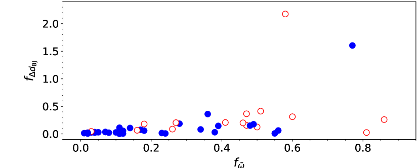
Figure 1: Fractional difference between the inverse of the Gaia DR2 parallax and the distance from Bailer-Jones et al. (2018), $f_{\Delta d_{\mathrm{BJ}}}$, as a function of the fractional error of the parallax $f_{\bar{\omega}}$. Filled circles indicate novae with known light curve type (Strope et al., 2010), open circles indicate those without.

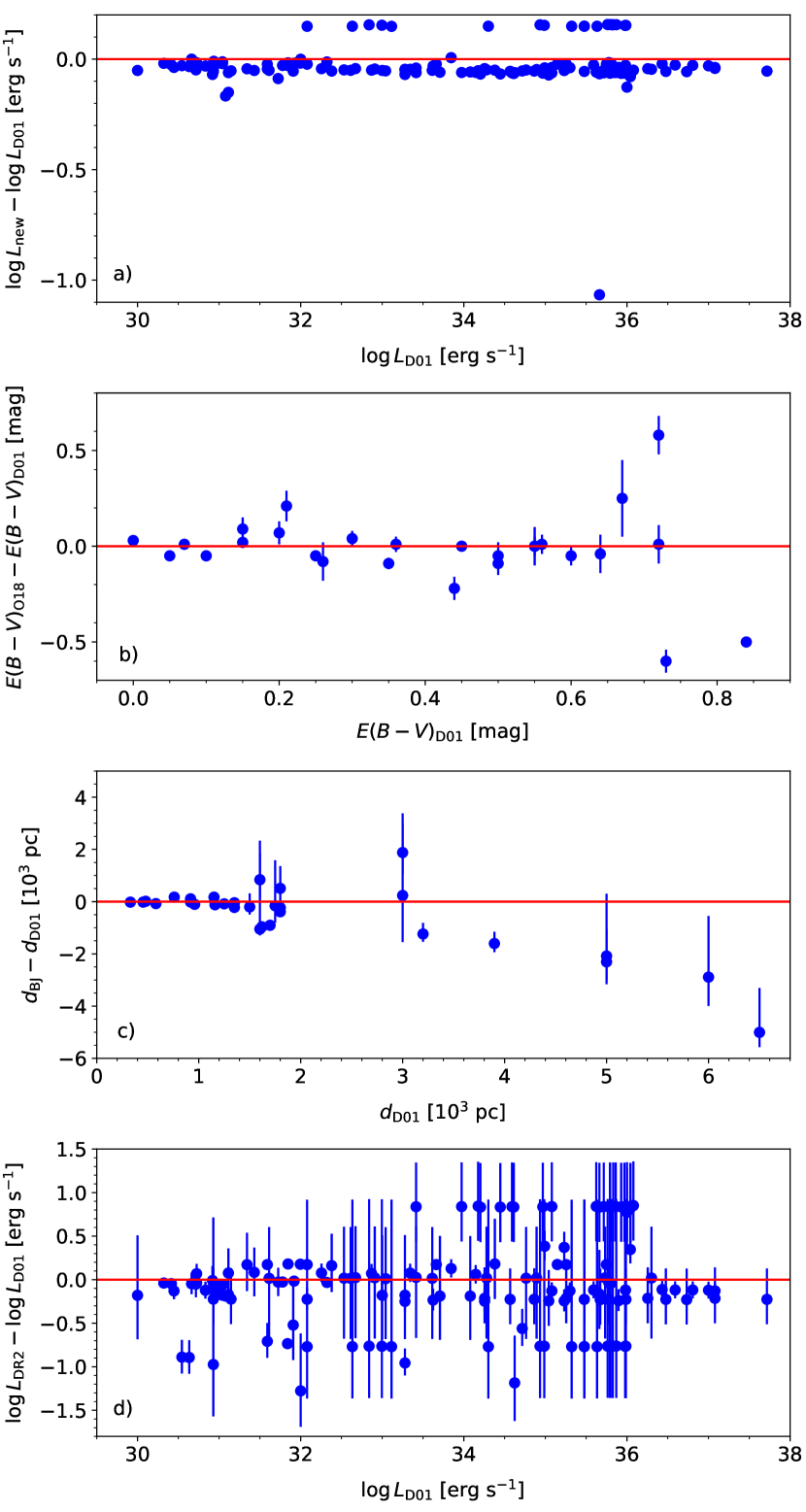
Figure 2: Comparison with the parameters used in D01. From top to bottom, the individual plots show a) the difference between the luminosities $L_{\mathrm{new}}$ calculated with Eq.1 using reddening and distances from D01 and the luminosities $L_{\mathrm{D01}}$, b) the difference between the reddening values $E(B-V)_{\mathrm{O18}}$ from Özdönmez et al. (2018) and $E(B-V)_{\mathrm{D01}}$, c) the difference between the distances $d_{\mathrm{BJ}}$ from Bailer-Jones et al. (2018) and $d_{\mathrm{D01}}$ , and d) the differences between the luminosities $L_{\mathrm{DR2}}$ calculated using $E(B-V)_{\mathrm{O18}}$ and $d_{\mathrm{BJ}}$ with $L_{\mathrm{D01}}$. All differences are plotted versus the respective values from D01.

The D01 catalogue lists the shell luminosities for the forbidden [Oiii] emission as well as for the hydrogen transitions H$\alpha$ and H$\beta$. In this work, for the sake of brevity and focus, we do not consider the H$\beta$ line because it will track basically the same, optically thicker, part of the shell as H$\alpha$, in contrast to [Oiii], which will correspond to optically thinner material. We chose H$\alpha$ over H$\beta$ because it is the stronger line, especially at later stages, and the corresponding flux measurements would be less affected by noise. The disadvantage of this choice is that the flux measured from a narrow-band filter centred on H$\alpha$ would potentially also include emission from the nearby [Nii] lines at $\lambda$654.8 and $\lambda$658.3 nm. However, for the vast majority of the nova shells, the combined flux of the [Nii] lines would still amount to less than the H$\alpha$ emission, so that the total flux would differ from the pure H$\alpha$ flux by less than a factor of two, which, for our purposes, is not relevant. Still, we should be aware that when in the following we talk about H$\alpha$ fluxes and luminosities, this actually means H$\alpha$ + [Nii].

The luminosity $L_{\lambda}$ of an emission at wavelength $\lambda$ can be calculated from the flux $F_{\lambda}$ as

$$L_{\lambda}=4\pi d^{2}F_{\lambda}\leavevmode\nobreak\ 10^{\frac{c_{\lambda}RE(B-V)}{2.5}},$$ (1)

where $d$ is the distance to the observer, $E(B-V)$ the reddening parameter, $R=3.1$ the extinction law parameter (Cardelli et al., 1989), and $c_{\lambda}=A_{\lambda}/A_{V}$ is the conversion factor between the wavelength specific absolute extinction $A_{\lambda}$ and the one in the visual range, $A_{V}$. We used the York Extinction Solver (McCall, 2004), employing the reddening law from Fitzpatrick (1999), to obtain the values for the two lines used in this work to $c_{\mathrm{H\alpha}}=0.75$ and $c_{\mathrm{[O\,III]}}=1.111$.

Apart from the luminosities, the D01 catalogue also provides information on the $d$, $E(B-V),$ and $F_{\lambda}$ values used for their calculation, however, as mentioned above, without including their associated uncertainties. With respect to the fluxes, only a few of the original source articles include error estimations (e.g. Ringwald et al., 1996). Additionally, a considerable part of the data is exclusive to the catalogue or is cited as ‘private communication’. Thus, we made the decision to take all flux data from D01 to avoid giving the impression that certain data points are more precise than others.

For the other two parameters, however, new measurements exist that also provide an estimation of the associated uncertainties. For the reddening data, we turned to the catalogue of Özdönmez et al. (2018), where available, while for the distances, we consulted the catalogue of Bailer-Jones et al. (2018), which is based on the Gaia Data Release 2 (hereafter DR2) parallaxes (Gaia Collaboration et al., 2018). For a few objects, there were also 3D reddening data available from the DR2 data via the Stilism website (Lallement et al., 2019), which were found to be in agreement with those of Özdönmez et al. (2018) within the errors.

The DR2 distances require some closer inspection. First of all, the novae used by D01 have to be cross-matched with the DR2 catalogue. This is less trivial than would otherwise be expected as most novae are located in the crowded regions of the Galactic disc, and even queries with radii as small as 2 arcsec can give ambiguous results. We have therefore compared each Gaia source with the available finding charts and, in a few cases, we used additional data to ensure the validity of a nova identification. Details on this process and the results for each nova included in D01 are given in Appendix A.

Secondly, also the distances themselves have to be evaluated beyond taking into account their formal uncertainties. The root of the problem here is the non-Gaussian distribution of the latter that results when calculating the distance as the inverse of the measured parallax $\bar{\omega}$, which becomes more pronounced and skewed the larger the uncertainty of the parallax measurement is in comparison to the value of the parallax. This not only affects the estimation of the uncertainty associated with the distance, but the distribution will also yield a most probable value for the distance that does no longer correspond to the true value (Luri et al., 2018). This problem can be addressed by interpreting the results in the context of a more realistic model of the distance distribution, for example, by using a prior according to Bayes’ theorem (Bailer-Jones, 2015), with the recommended approach being to assume an exponentially decreasing space density (EDSD; Luri et al., 2018). This was done by Bailer-Jones et al. (2018), who used a length scale map based on a chemo-dynamical model of the Galaxy (Rybizki et al., 2018) to estimate the distances of the Gaia DR2 sources, and by Schaefer (2018), who used a less complex approach of a length scale model as a function of the galactic latitude to derive distances for a sample of 64 novae.

Still, we are not out of the woods yet because the resulting distances continue to be affected by the uncertainties of the parallax measurements $\sigma_{\bar{\omega}}$ in a non-uniform way. Bailer-Jones (2015) has shown that for fractional errors $f_{\bar{\omega}}\equiv\sigma_{\bar{\omega}}/\bar{\omega}>0.373$ the assumed prior starts to dominate the distance estimation, that is, the resulting value is more determined by the assumed model than by the actual parallax measurement. Thus, to be on the safe side, we should limit our sample to novae with fractional errors below this value. However, we have to consider that this could diminish the size of our sample to a number where it loses statistical significance. In addition, the luminosity range that is covered by the data spreads over several orders of magnitude (D01), so that even a very uncertain distance might still prove useful for our purposes. Thus, we decided to define our sample based on the Gaia DR2 information applying three criteria.

Firstly, we exclude all objects with negative parallaxes because while they can be formally used to calculate distances, a comparison with data for clusters shows that such distances present a systematic offset (Bailer-Jones et al., 2018). Secondly, for similar reasons, we exclude distances with fractional errors, $f_{\bar{\omega}}\geq 1,$ because these allow for negative or zero parallaxes within the uncertainties. Thirdly, in order to estimate the influence of the prior on the distance value, we compare the distance, $d_{\bar{\omega}}$ , calculated as the inverse of the parallax to the distances computed with a Bayesian prior, $d_{\mathrm{BJ}}$ and $d_{\mathrm{S}}$, from Bailer-Jones et al. (2018) and Schaefer (2018), respectively, by defining absolute fractional differences, namely,

$$f_{\Delta d_{\mathrm{BJ}}}\equiv|d_{\mathrm{BJ}}-d_{\bar{\omega}}|/d_{\bar{\omega}},$$ (2)

and $f_{\Delta d_{\mathrm{S}}}$ , correspondingly. Figure 1 shows $f_{\Delta d_{\mathrm{BJ}}}$ as a function of $f_{\bar{\omega}}$. For clarity, we have omitted the values for V1419 Aql, which has $f_{\bar{\omega}}=0.33$ and $f_{\Delta d_{\mathrm{BJ}}}=16.1$, and actually represents a good example for the fractional error alone not being a sufficient quality criterion. Based on that plot, we set our limit to $f_{\Delta d_{\mathrm{BJ}}}<0.5$, since below that value, the distribution is comparatively uniform for $f_{\bar{\omega}}>0.2$. This means that the use of a prior does not result in a distance difference larger than a factor of two compared to not using a prior and also means that the corresponding luminosity is affected by a factor of $\leq$4, which should still represent a reasonable uncertainty considering the luminosity spread. While not shown here explicitly, we performed the same comparison with the Schaefer (2018) distances and obtained similar results. Specifically, we found that all objects with $f_{\Delta d_{\mathrm{BJ}}}<0.5$ also have $f_{\Delta d_{\mathrm{S}}}<0.5$ and vice versa, which proves the consistency of this limit.

For several objects, we applied additional criteria. The recurrent novae RS Oph and V3890 Sgr formally are within our limits. However, both objects contain giant secondary stars and have comparatively long periods. Schaefer (2018) argues that the resulting orbital wobble is of the same size as the measured parallax, thus rendering the latter inapplicable. Because there is a decent amount of luminosity data available for these two objects, and because the behaviour of the flux data within themselves for a particular system is independent of the distance, we included these objects for comparison, but we ought to keep in mind that the zero point on the luminosity axis for those two objects is undetermined. As for the other recurrent nova, T Pyx, there is only one very late data point, whose placement on the time axis is uncertain since Schaefer et al. (2010) argue that the observed shell is a remnant of an eruption in the year 1866, instead of the one in 1967. In our analysis, we therefore treat these objects with the appropriate caution and we do not attempt to fit the data.

Finally, the nova V838 Her with $f_{\bar{\omega}}=1.53$ does not qualify. However, as we will see below, there is no reasonably possible distance value that could reconcile its luminosity decline with any of the other objects, and so it will be discussed individually, making the assigned distance less important. In contrast to the cases of RS Oph and V3890 Sgr, here the distribution of the points is such that it allows for a meaningful linear fit. These steps resulted in a sample of 42 objects with associated DR2 distances from the Bailer-Jones et al. (2018) catalogue and then further reduced to 29 objects which have a light curve type assigned (see Section 3).

In order to evaluate the consequences of employing these new sets of parameters, we compared them to those listed in D01. Firstly, however, we calculated the H$\alpha$ luminosities using the D01 parameters to check for potential inconsistencies in the catalogue itself. In the top plot of Fig. 2 we present the difference between such newly calculated luminosities, $L_{\mathrm{new}}$ ,using Eq.1 and the values $L_{\mathrm{D01}}$ listed in the catalogue as a function of the latter. We see that the bulk of the points lies slightly below the zero line, which can be easily explained by the use of a different reddening law and corresponding conversion factor, $c_{\mathrm{H\alpha}}$, and the scatter within this bulk is likely due to rounding. For deviating points farther off this bulk, we can only speculate that this is because the parameters used for the calculation do not correspond to those listed in the paper, perhaps due to mistakes in the transcription. This would either concern reddening or distances, affecting all data points of a particular object (e.g. the row of points at $\sim$0.15 on the y-axis corresponds to all the V2214 Oph data) or individual data (e.g. the most deviating point corresponds to one out of 25 data points for V992 Sco and is clearly a typographical mistake in the exponent of the stated luminosity).

In the upper middle plot, we show the comparison with the reddening values $E(B-V)_{\mathrm{O18}}$ from Özdönmez et al. (2018). We find that for $E(B-V)_{\mathrm{D01}}\leq 0.6$ mag, they match well, while for stronger reddening, there is a considerably larger scatter. The strongest deviating points with absolute differences $>$0.5 mag are those of V888 Cen, BY Cir, and V992 Sco. For the first two of those, D01 have used the maximum magnitude vs rate of decline relationship (MMRD) for classical novae to derive distance and reddening. However, this method, at least in its past form, is considered unreliable today (e.g. Schaefer, 2018; Selvelli & Gilmozzi, 2019). For V992 Sco, D01 also quote their own work, but they do not specify how the reddening was obtained. In all three cases, we thus consider the Özdönmez et al. (2018) reddening as more trustworthy.

Next, in the lower middle plot, we compare the distances. There is a generally good agreement between the D01 values $d_{\mathrm{D01}}$ and those of DR2 for $d_{\mathrm{D01}}\leq 1500$ pc, after which the scatter becomes larger, but still stays within the uncertainties of the DR2 data. For $d_{\mathrm{D01}}>3000$ pc, the D01 values appear to be systematically larger than those of Bailer-Jones et al. (2018). The largest deviation is observed for DO Aql, which is an interesting case, since, as noted by D01, a proper application of the MMRD would have resulted in an even larger distance of 9.5 kpc, while a comparison with the faintest novae would place it at 3.6 kpc, the latter at least being comparable with the DR2 distance $d_{\mathrm{BJ}}=1.5^{+1.7}_{-0.6}$ kpc within the uncertainties. Finally, D01 decided to take the average of the two extremes.

Concluding the comparison, the bottom plot of Fig. 2 presents the difference between the D01 data and the new luminosities that were calculated using the reddening from Özdönmez et al. (2018) and the DR2 distances from Bailer-Jones et al. (2018). The differences between the two sets of luminosities can be considerable, amounting up to around one order of magnitude. From the other plots, and also from Eq.1, it is clear that these are mainly due to the differences in the distance estimates.

2.2 Ancient novae

As mentioned briefly in the introduction, there are now ten cases where the presence of a nova shell has revealed a previous nova eruption in a CV where the eruption itself was not observed. For the lack of a more precise and poignant term, we call those systems ‘ancient novae’, although this should not be taken strictly in the sense of an age indicator. Still, typically these nova eruptions will have occurred in epochs that predate the known nova eruptions and could, perhaps, be dated in some cases if a historical Far Eastern Guest star can be identified with a modern CV as classical nova candidate (Vogt et al., 2019; Hoffmann, 2019). Determining the luminosity of their shells would, thus, extend the time axis beyond the D01 data and provide important information on the late stages of the luminosity evolution. In the following, we inspect nine of these cases, focussing on the available data regarding age and shell luminosity, and using the DR2 distances from Bailer-Jones et al. (2018) and the Stilism reddening (Lallement et al., 2019) in the process (see Tables LABEL:allD01_tab and 4). We note that not all systems can be used for our purposes, but we still include them for completeness. The tenth ancient nova is a member of the globular cluster M22 (Göttgens et al., 2019). Because of the possibility that the formation and evolution of CVs in globular clusters is particular to the conditions in the cluster (Knigge, 2012; Belloni et al., 2016, 2017a, 2017b, 2019) and that they are not representative, thus, for the general population of CVs, we do not consider such objects further.

2.2.1 V1315 Aql

This is a nova-like variable of the SW Sex sub-type (Hellier, 1996), which is suspected to harbour the CVs with the highest mass-transfer rates (Rodríguez-Gil et al., 2007; Townsley & Gänsicke, 2009; Schmidtobreick, 2015). The shell was detected by Sahman et al. (2015) in an H$\alpha$ survey. A preliminary age estimate of 120 yr was later corrected to a possible age range of 500 to 1200 yr, strongly depending on the original velocity of the ejecta (Sahman et al., 2018). Here, we will assume a mean value of 850 $\pm$ 350 yr. The authors calculate a total flux for H$\alpha$ to $F=2.5(6)\times 10^{-13}$ erg cm^-2 s^-1. From their Table 4, we can estimate that the combined flux of the neighbouring [Nii] lines amounts to roughly 2/3 of that value, so that a typical narrow band filter centred on H$\alpha$ would yield an overall flux of about $4.2(7)\times 10^{-13}$ erg cm^-2 s^-1, implying $L=1.3^{+0.5}_{-0.4}\times 10^{31}$ erg s^-1.

2.2.2 V341 Ara

V341 Ara is one of the brightest CVs on the sky, but it was only recognised as such relatively recently (Frew, 2008; Bond & Miszalski, 2018). It is associated to an H$\alpha$ emission nebula and the authors referenced above list a nova eruption as one of the potential scenarios, with the proper motion data implying an age of the nova of about 800 yr. Adding up the fluxes from [Nii] and H$\alpha$ given by Frew (2008) yields a combined flux $F=6.4\times 10^{-14}$ erg cm^-2 s^-1. Using the DR2 and Stilism data on distance and reddening distribution, respectively, yields $L=2.0^{+0.2}_{-0.1}\times 10^{29}$ erg s^-1. For [Oiii] the corresponding values are $F=5.5\times 10^{-14}$ erg cm^-2 s^-1 and $L=1.8^{+0.2}_{-0.1}\times 10^{29}$ erg s^-1.

2.2.3 Z Cam

This was the first CV unmasked as an ancient nova (Shara et al., 2007) and it is still the oldest, with an estimated age of 1300 to $\geq$5000 yr (Shara et al., 2012b). It has been suggested that it can be identified with a guest star from the year 77 BCE as recorded by Chinese astrologers (Johansson, 2007), but this has been recently disputed by Hoffmann (2019). Unfortunately, the Z Cam shell so far has only been analysed in terms of extension and expansion, but not in flux, so that it cannot be used in the context of the present paper.

2.2.4 BZ Cam

The most recently found coincidence of a CV with a possible nova shell refers to this nova-like variable of VY Scl sub-type with an orbital period of 3.7 h (Honeycutt et al., 2013). Hoffmann & Vogt (2020) report that BZ Cam could be the counterpart of an ancient guest star observed by Chinese astronomers in the year 369 CE, and that it seems to be associated to the faint nebula EGB 4, a planetary nebula candidate with a multiple structure (Ellis et al., 1984). BZ Cam is situated at the edge of a red nebula (apparently caused by H$\alpha$ emission) and surrounded by a smaller bluish [Oiii] nebula, implying a nova shell. Based on the DR2 distance and proper motion values of BZ Cam, Hoffmann & Vogt (2020) estimate that the shell structure could have witnessed a total of three past ejection episodes, about two, five and eight millennia ago. It could be the first candidate for a recurrent nova with extremely long repetition cadence.

Greiner et al. (2001) estimated the total [Oiii] flux of the nebula to $F=4.8\times 10^{-13}$ erg cm^-2 s^-1, while Krautter et al. (1987) gave $F=4.3\times 10^{-13}$ erg cm^-2 s^-1 and $F=1.3\times 10^{-13}$ erg cm^-2 s^-1 for the eastern and western part of the nebula, respectively, which, in total, thus yields a slightly higher value, but stays within the same order of magnitude. The spatial distribution of the H$\alpha$ and [Oiii] fluxes is highly inhomogeneous. From the data given in Hollis et al. (1992), Krautter et al. (1987) and Greiner et al. (2001), we estimate a rough average of $F(\mathrm{[OIII]})/F(\mathrm{H}\alpha+\mathrm{[NII]})\sim 1.7$ for the flux ratio of the lines relevant for our study. With the flux value for [Oiii] from Greiner et al. (2001) given above and their stated uncertainty of 20%, we thus estimate a corresponding flux for H$\alpha$ to $F=2.8(6)\times 10^{-13}$ erg cm^-2 s^-1, yielding luminosities of $L=5.1^{+1.9}_{-1.5}\times 10^{30}$ erg s^-1 for H$\alpha$ and $L=9.1^{+3.9}_{-3.0}\times 10^{30}$ erg s^-1 for [Oiii].

2.2.5 AT Cnc

The shell around this Z Cam sub-type dwarf nova was discovered by Shara et al. (2012a) and later analysed in more detail by Shara et al. (2017b). The authors estimate the age of the nova as 330${}^{+135}_{-90}$ yr. The emission of the shell is dominated by forbidden transitions, with very little contribution from hydrogen, if any. The flux measured with a narrow band filter on H$\alpha$ will thus mostly correspond to the $\lambda$654.8 and $\lambda$658.3 nm [Nii] emission. Adding up the flux of all the emission blobs measured by Shara et al. (2017b) yields $F=3.3(3)\times 10^{-14}$ erg cm^-2 s^-1. The corresponding luminosity then calculates to $L=8.5\pm 1.3\times 10^{29}$ erg s^-1.

2.2.6 V1363 Cyg

Sahman et al. (2015) present an H$\alpha$ image that shows possible traces of a nova shell centred on this dwarf nova, with its proximity to a gas cloud impeding an unambiguous identification. To our knowledge, no further analysis of this potential shell has been undertaken so far. While there is thus no further use for this system within the scope of our study, we allow ourselves a brief tangent, taking advantage of the availability of a good distance measurement. The projected radius of the potential shell is estimated to 60 arcsec (Sahman et al., 2015). With $d_{\mathrm{BJ}}=1.7\pm 0.1$ kpc, this translates to an absolute extension $r=0.49\pm 0.03$ pc. In the attempt to estimate the age of a nova shell, it is often considered that an original expansion velocity in the order of $\sim$2000 km/s decreases exponentially with a half-life of $\sim$75 yr, which is based on a study of four nova shells by Duerbeck (1987) and which is thought to be caused by interaction with the surrounding interstellar medium (Oort, 1946). In the case of V1363 Cyg, these values do not agree with the observed extension of the shell, requiring either a considerably higher ejection velocity $>$4000 km/s or a longer half-life $>$100 yr. In a recent study of five shells, Santamaría et al. (2020) did not find any compelling evidence for deceleration, and if the feature in the H$\alpha$ images of V1363 Cyg indeed corresponds to a nova shell, this might be another example for above rule of thumb not being applicable in a general way.

2.2.7 CRTS J054558.3+022106

This eclipsing dwarf nova was detected within the suspected planetary nebula Te11, which, based on this discovery, was then reinterpreted as an ancient nova shell (Miszalski et al., 2016). The authors identify the nova eruption with a guest star recorded at the end of the year 483 CE, which, according to Hoffmann (2019), is possible, but ambiguous. Miszalski et al. (2016) report an H$\alpha$ flux $F=2.4\times 10^{-13}$ erg cm^-2 s^-1, which is likely to represent a close lower limit, because their aperture photometry did not encompass the full nebula. From their Table 3, we estimate a flux for [Oiii] $F=2.5\times 10^{-13}$ erg cm^-2 s^-1. Unfortunately, the DR2 parallax is accompanied by a large uncertainty of almost 1 mas. The corresponding distances are $d_{\bar{\omega}}=0.6^{+1.1}_{-0.2}$ pc and $d_{\mathrm{BJ}}=1.0^{+1.2}_{-0.5}$ kpc, which yields $f_{\Delta d_{\mathrm{BJ}}}=0.67,$ which is, thus, above our quality limit for the distance and so, the luminosity calculation (Section 2.1). Miszalski et al. (2016) derive $d=330(50)$ pc based on the flux and spectral type estimations of the donor star in the dwarf nova system. However, they also give a reddening $E(B-V)=0.32$ mag, and according to the Stilism data, this definitively implies $d>550$ pc, with the values presenting a comparatively narrow transition in the reddening distribution just below 500 pc, where $E(B-V)$ rises from $<$0.1 to $\geq$0.29 mag within 50 pc. For a very rough estimate, we use the lower limit of 550 pc as implied by the reddening, and a maximum of 2.2 kpc as indicated by the $d_{\mathrm{BJ}}$ formal distribution to obtain $L\sim 1.1^{+1.7}_{-0.9}\times 10^{32}$ erg s^-1. The corresponding value for [Oiii] results to $L\sim 1.6^{+2.4}_{-1.3}\times 10^{32}$ erg s^-1.

2.2.8 IGR J17014$-$4306

Another eclipsing dwarf nova and possible intermediate polar (Potter & Buckley, 2018), this object has been associated by proper motion analysis with a nebula and a guest star sighting in the constellation of Scorpius recorded by Korean observers in 1437 CE (Shara et al., 2017c). The latter has been recently challenged by Hoffmann (2019) who, based on a reanalysis of the historical texts, argues that the position of the guest star does not agree with the location of the nebula. However, since a comparison with the proper motion of the binary and the centre of the nebula yields a comparable time scale, here we assume an age of $\sim$600 yr. This is sufficient for our purpose, considering that we compare on a logarithmic scale. Shara et al. (2017c) give a combined H$\alpha$ + [Nii] flux $F=2.8\times 10^{-12}$ erg cm^-2 s^-1, which yields a luminosity of $L=7.4^{+3.2}_{-2.2}\times 10^{32}$ erg s^-1.

2.2.9 IPHASX J210204.7+471015

This is a nova-like variable with a likely orbital period of 4.3 h (Guerrero et al., 2018). Santamaría et al. (2019) estimate the age of the shell to 147(20) yr. From Table 4 in Guerrero et al. (2018), we derive a combined H$\alpha$ + [Nii] flux $F=4.4\times 10^{-14}$ erg cm^-2 s^-1, which, with the DR2 and Stilism data, implies $L=5.0^{+1.5}_{-1.2}\times 10^{30}$ erg s^-1. Similarly, for [Oiii] $\lambda$500.7 nm, $F=2.7\times 10^{-15}$ erg cm^-2 s^-1 and $L=4.1^{+1.8}_{-1.3}\times 10^{29}$ erg s^-1.

3 Luminosity evolution

Table 1: Distribution of the novae in our sample among speed classes (rows) and light curve types (columns). The final row and column gives the total number of entries in a specific light curve type and speed class, respectively.

	D	F	J	O	P	S	$n_{\mathrm{SC}}$
VF	1	0	0	2	1	2	6
F	2	0	1	1	3	3	10
MF	6	0	0	0	0	1	7
SVS	0	2	4	0	0	0	6
$n_{\mathrm{LCT}}$	9	2	5	3	4	6	(29)

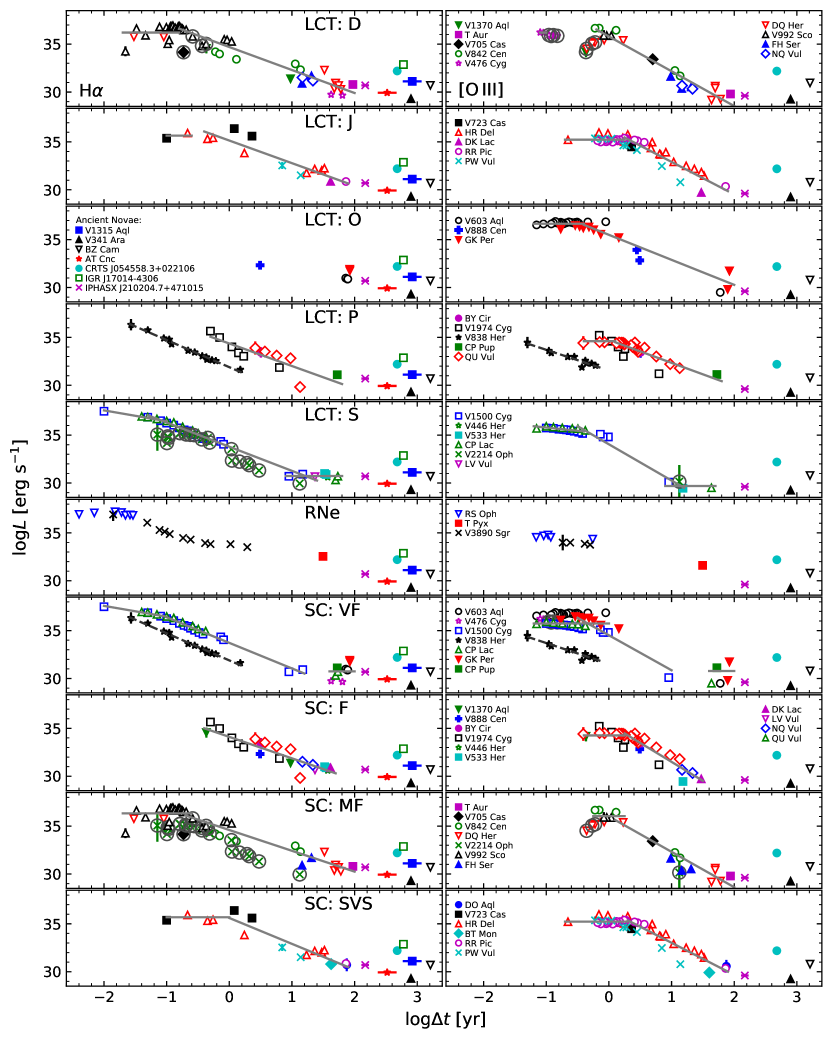
Figure 3: H$\alpha$ (left panels) and [Oiii] (right panels) emission line luminosities as a function of the time that has passed since maximum brightness. Both parameters are shown in logarithmic scaling. The novae are grouped either with respect to their light curve type (LCT) or speed class (SC). The ancient novae have been incorporated in all plots, for comparison. The symbol identifications correspond to the respective plots of both emission lines. Symbols enclosed in larger grey circles indicate data points that were excluded from the fit. Error bars are shown only for the first data point of a respective object. Solid light grey lines represent linear fits to the data of a specific group, the dashed darker grey line shows the fits to the V838 Her data.

Table 2: Parameters $a$ and $b$ of the linear fits according to Eq. 3. $\Delta(\log\Delta t)$ gives the time range of the corresponding segment, with $\Delta t$ in yr, $n$ is the number of data points used in the fit, and $\sigma$ is the standard deviation of the linear regression. For a few groups, two rows are given for the same interval. The first corresponds to the linear fit, while the second states the mean value for $b$, setting the slope $a$ to zero.

Class	$\Delta(\log\Delta t)$		$n$	$b$	$a$	$\sigma$
H$\alpha$
D	$-$1.7 ..	$-$0.8	15	36.21(21)	0	0.79
	$-$0.8 ..	2.0	28	34.70(14)	$-$2.40(13)	0.64
J	$-$1.0 ..	$-$0.6	2	35.65(27)	0	0.27
	$-$0.4 ..	1.9	13	35.14(35)	$-$2.36(31)	0.81
P	$-$0.3 ..	1.8	13	34.36(32)	$-$2.35(43)	0.82
S	$-$2.0 ..	$-$1.0	8	35.32(17)	$-$1.13(13)	0.11
	$-$2.0 ..	$-$1.0	8	36.76(13)	0	0.35
	$-$1.3 ..	1.4	24	33.79(06)	$-$2.52(06)	0.22
	0.9 ..	1.8	8	30.73(07)	0	0.20
V838 Her	$-$1.6 ..	0.2	13	31.89(07)	$-$2.83(09)	0.14
VF	$-$2.0 ..	$-$1.0	8	35.32(17)	$-$1.13(13)	0.11
	$-$2.0 ..	$-$1.0	8	36.76(13)	0	0.35
	$-$1.0 ..	1.2	19	33.72(06)	$-$2.67(08)	0.21
	1.6 ..	2.0	7	30.74(32)	0	0.83
F	$-$0.4 ..	1.7	22	34.11(23)	$-$2.24(24)	0.69
MF	$-$1.7 ..	$-$0.6	21	36.33(15)	0	0.70
	$-$0.7 ..	2.0	18	34.59(24)	$-$2.17(19)	0.71
SVS	$-$1.0 ..	0.0	5	35.69(18)	0	0.41
	0.0 ..	1.9	12	35.61(49)	$-$2.70(38)	0.78
[Oiii]
D	$-$0.2 ..	2.0	21	35.80(22)	$-$3.63(20)	0.66
J	$-$0.7 ..	0.25	23	35.23(06)	0	0.28
	0.25 ..	1.9	23	36.30(31)	$-$3.39(32)	0.72
O	$-$1.2 ..	$-$0.4	21	36.66(05)	0	0.21
	$-$0.4 ..	2.0	12	35.50(34)	$-$2.61(31)	0.97
P	$-$0.4 ..	0.1	6	34.60(12)	0	0.29
	0.1 ..	1.8	26	34.73(16)	$-$2.39(27)	0.50
S	$-$1.2 ..	$-$0.4	15	35.11(13)	$-$0.68(17)	0.14
	$-$1.2 ..	$-$0.4	15	35.61(05)	0	0.19
	$-$0.5 ..	1.2	9	34.04(16)	$-$3.78(28)	0.50
	0.9 ..	1.7	3	29.69(17)	0	0.29
V838 Her	$-$1.3 ..	$-$0.2	10	31.54(16)	$-$2.16(24)	0.25
VF	$-$1.2 ..	0.0	27	35.74(08)	0	0.40
	$-$0.5 ..	1.0	14	34.51(21)	$-$3.65(52)	0.71
	1.6 ..	2.0	5	30.78(43)	0	0.95
F	$-$0.4 ..	0.25	17	34.26(12)	0	0.49
	0.25 ..	1.5	23	35.46(23)	$-$3.96(31)	0.55
MF	$-$0.25 ..	0.25	8	36.04(17)	0	0.48
	0.1 ..	2.0	13	36.00(50)	$-$3.69(38)	0.76
SVS	$-$0.7 ..	0.3	26	35.23(06)	0	0.31
	0.3 ..	1.9	21	36.37(34)	$-$3.35(31)	0.68

In their investigation of the luminosity evolution, D01 distinguished between different speed classes. In the present work, we also want to examine a possible correlation with the light curve type as defined by S10. To be able to conduct a proper comparison for the two different groupings, we limit the sample to those objects in D01 that also have a light curve type assigned.

The speed class system used by D01 is that of Payne-Gaposchkin (1964) who defined the following intervals for $t_{2}$: up to 10 d (Very Fast, VF), 10 to 25 d (Fast, F), 26 to 80 d (Moderately Fast, MF), 81 to 150 d (Slow, S) and from 151 d on (Very Slow, VS). D01 do not strictly follow that scheme, but take, rather, $t_{3}$ as a second indicator whenever there is a significant break in the decline law. For example, V723 Cas, with $t_{2}$ = 19 d and $t_{3}$ = 180 d would be classified as Slow instead of Fast. However, this introduces some personal ambiguity (and furthermore emphasises the weakness of a scheme that tries to categorise nova light curves using one or two decline rate parameters). There are also some inconsistencies in the catalogue; for example, V446 Her with $t_{2}$ = 7 d and $t_{3}$ = 12 d is classified as Fast, while GK Per with identical $t_{2}$, but $t_{3}$ = 13 d is labelled as Very Fast. To make a proper comparison possible, we decided to use the speed classes assigned by D01, regardless of the actual decline rate parameters. Furthermore, we follow their scheme of combining the two slow classes and hereafter, we refer to the latter as SVS.

In contrast, S10 used purely phenomenological criteria to characterise the decline light curves of novae and to define seven different types based on their distinctive features. In our sample, we found members of six of these types: D (Dust Dip), F (Flat Top), J (Jitter), O (Oscillations), P (Plateau), and S (Smooth). Only the least frequent class, C (Cusp, which S10 find to include only 1% of the novae), is not represented in our sample. However, we will also have to disregard the second least frequent one, F (2%), because there are only two members (BT Mon and DO Aql), each of which counts with only a single data point per emission line.

In Table 1, we compare the distributions of the different novae of our sample both for speed class and for light curve type to see whether these two different groupings are indeed independent from each other. We do find a rough correlation, with the O, P, and S light curve types showing a concentration towards faster speed classes, while the D and J types include slower novae. We note that although the small numbers per individual bin suggests we should use some caution when considering the significance of this result, it quite faithfully, in fact, reflects the distribution in the S10 catalogue itself. Thus, if the rate of decline of the broad-band photometric nova brightness (i.e. the speed class) were the dominant parameter also for the shell luminosity and its evolution, we would expect very similar behaviour for those light curve types that sample similar speed class regimes, that is,  O, P, and S on the one side and D and J on the other.

The parameters that were used to calculate the luminosities as well as the grouping criteria of all novae in our sample are given in the appendix in Table 4. The resulting luminosities $L$ of the different groupings are shown in Fig. 3 as a function of the time $\Delta t$ that has passed since the maximum brightness of the eruption. The errors propagate only from the uncertainties in the distance and reddening measurements and, thus, they are identical for each data point for a given nova. Therefore, they do not affect the general tendency of specific systems but they do indicate possible displacements of that tendency along the luminosity axis. As a result, we chose to include the error bars only in the first data point of a nova in the plots. Following the example of D01, we divide the distributions into segments with linear behaviour on the logarithmic scale and fitted linear functions,

$$\log L=a\log{\Delta t}+b$$ (3)

to them, with $L$ in erg s^-1 and $\Delta t$ in yr. The limits of the $\log\Delta t$ range of a particular segment were determined by eye. In cases where the slope was consistent with a zero value within the errors, it was set to zero, with the $y$-axis intersection $b$ corresponding to the average of the data points in that segment. In Table 2, we give the details of the segments and the fit parameters. The H$\alpha$ data for the O light curve type were found too sparse to yield a meaningful fit. The results and their implications are discussed in Section 4. In the following, we remark briefly on a few noteworthy topics and objects.

Dust Dips: The D light curve type is defined by presenting a significant isolated minimum in the post-eruption light curve. This feature is caused by dust absorption and has been found to also affect line emission (Shore et al., 2018). In our data, this is especially evident in the [Oiii] data of DQ Her (top right panel of Fig. 3), where a comparison with the broad-band light curve in S10 (their figures 2 and 7) shows that the first three of our data points coincide with the final phases of the dust dip. Because of the distorting effect on the general decline behaviour, time ranges corresponding to such broad-band photometric dust dips were excluded from the fits, both in the D type and in the speed class groupings. This concerns the novae V476 Cyg, DQ Her, and V992 Sco.

V1370 Aql: This nova also belongs to the D light curve type. However, the comparison with S10 (where it is mislabelled in the plots as V1370 Cyg) shows that all data points lie clearly outside the visual dust feature. Nevertheless, the [Oiii] data point, in particular, presented a significantly diminished luminosity compared to the rest of the D group. Upon further investigation, we indeed found a discrepancy between the flux values quoted by D01 and those of the original source corresponding to the time $\Delta t$ = 0.43 yr (Snijders et al., 1987). There, two flux values are given per emission line that correspond to an identified broad and narrow component. For H$\alpha$, these are $F_{b}=8.0\pm 1.0\times 10^{-12}$ erg cm^-2 s^-1 and $F_{n}=2.0\pm 0.5\times 10^{-12}$ erg cm^-2 s^-1, respectively, while the fluxes for [Oiii] $\lambda$500.7 nm are given as $F_{b}=2.0\pm 0.5\times 10^{-12}$ erg cm^-2 s^-1 and $F_{n}=0.2\pm 0.1\times 10^{-12}$ erg cm^-2 s^-1. In comparison, D01 state $F=2.0\times 10^{-12}$ erg cm^-2 s^-1 for H$\alpha$ and $F=2.9\times 10^{-13}$ erg cm^-2 s^-1 for [Oiii]. The only way that we can seek to reconcile these data with the original source is the explanation that D01 chose to only consider the narrow components and, additionally, they made a mistake in the transcription of the [Oiii] flux (e.g. 2.9 instead of 2.0). Yet even if that were the case, the choice for the narrow component is peculiar, considering that Snijders et al. (1987) view the broad component as more likely to correspond to the ejected material. Because the grouping also puts together spectroscopic and photometric data, here we decided to replace the D01 values with the combined fluxes from Snijders et al. (1987).

Still, while in the Fast speed class groupings and also in the H$\alpha$ D type plot, the revised data now agree with the general distribution, the [Oiii] luminosity remains too low by at least two orders of magnitude when compared to the other D type members V476 Cyg and V842 Cen, as it lies even slightly below the very first (dust) data point of DQ Her. Because it clearly represents an outlier and would have a disproportionally large effect on the fit, it was excluded.

V838 Her: This nova is classified as a P light curve type and as a member of the very fast speed class. However, its luminosity slope deviates from the general behaviour in both groups. As shown in Section 2.1, the distance to V838 Her cannot be reliably determined. However, from Fig. 3, it is clear that not only is the luminosity too low by about two orders of magnitude, requiring a larger distance by a factor of 10 to correct that displacement, but also that the decline starts significantly earlier than for the other systems. Thus, there is no distance value that would allow to reconcile its behaviour with those of the other novae. The large amount of flux data for this object makes it possible to discuss it independently (see Section 4.6).

BT Mon: D01 do not assign any speed class to this nova. However, the decline rate indicators $t_{2}$ and $t_{3}$ were determined by S10 to 118 and 182 d, respectively, which clearly indicates a slow nova. We have included the data points of BT Mon in the respective plots of this speed class, where it appears to agree reasonably well with the general distribution.

V2214 Oph: S10 place this nova among the S light curve types. However, looking at the broad-band light curve in their Figure 3, this object is clearly the one of the 32 members of this class that fits the description of a smooth decline the least, presenting instead a number of minima and maxima that deviate significantly from the average decline law. As can be seen in the respective panel in Fig. 3, the H$\alpha$ data present a very similar behaviour. We consider V2214 Oph as a very uncertain member of the S light curve class and thus we exclude it from the corresponding fits.

4 Discussion

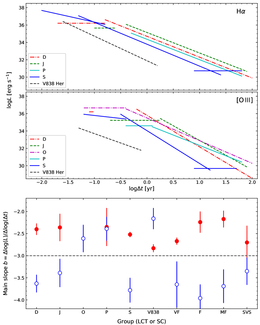
Figure 4: Comparison of the fits as defined in Table 2. For the sake of clarity, we omit the speed classes. The bottom plot compares the main decline slopes of all groups (filled circles = H$\alpha$, open circles = [Oiii]). The horizontal dashed line marks a slope of $-$3.0.

4.1 General description

The interpretation of the data and the corresponding fits in Fig. 3 call for a very cautious approach due to the fact that several regions in these distributions are severely undersampled. While there appears to be sufficient justification for separating the data into a number of sections and to apply a linear fit to each of them (which, of course, represents only a first approximation to a necessarily smooth continuous function), the choice of the corresponding time ranges is often ambiguous. Still, in general terms, the tendency is very similar for all groups. An initial, constant or very gentle slope is followed by a main decline that for H$\alpha$ starts at $\log\Delta t\leq$0.0 (i.e. $\leq$1 yr after the eruption), and for [Oiii] at $\leq$0.48 ($\leq$3 yr). The S light curve type and the Very Fast Speed Class additionally present another late, approximately constant behaviour. However, we note that while it is only in these two groupings that this late stage is obvious, in fact, the distributions in all groups are sufficiently ambiguous to allow, in principle, for the existence of such behaviour from $\log\Delta t\approx$1.5 (30 yr) onwards. D01 also remarked on that stage, but discarded it as being likely to have been caused by the emission from the accretion disc in the system becoming the dominant emission source. However, firstly, we find this behaviour also likely to be present in [Oiii], that is, in an emission that is exclusive to the shell. Secondly, especially in the later time ranges ($\Delta t>$ 30 yr), the nebular remnant of those novae is already spatially resolved. For example, the most distant novae in our sample that can be suspected to show this behaviour are CP Lac and V533 Her, with $d=$ 1.13 kpc and 1.17 kpc, respectively. Even assuming a comparatively slow expansion of 500 km s^-1, their shells will have projected diameters of about 5 arcsec. Thus, a contamination by emission from the accretion disc appears unlikely. Finally, the ancient nova data are consistent with the idea that there is another break in the decline law at late stages, with the slope being significantly diminished with respect to the main decline.

Taking all the above mentioned uncertainties into account, we suggest that the luminosity evolution of all groups can be cautiously described as experiencing an initial gentle decline, followed by a main steeper one, which, at late stages, again returns to a much softer slope. Because of the ambiguity in defining the time ranges of a specific phase, we do not regard the differences in the times of transition from one phase to another for different groups as significant as far as it concerns a specific emission line.

4.2 The main decline

We start our exploration of the physics behind the luminosity evolution with the main decline because the initial stage can be best described by recognising the differences to the former.

From Table 2 and Fig. 4, we see that for H$\alpha$, all groups present very similar slopes. For the light curve types, we find a weighted mean of $\bar{a}_{\mathrm{LCT,H\alpha}}=-2.46(05)$ and for the speed classes $\bar{a}_{\mathrm{SC,H\alpha}}=-2.49(07)$. For the [Oiii] emission, the scatter is larger. Taking the weighted mean of all light curve types yields $\bar{a}_{\mathrm{LCT,[O\,III]}}=-3.20(12)$. However, we note that there are two groups that deviate significantly from this value. In the O types, this might be due to the main decline being less well-defined as for the other groups, which is due to a lack of data in the comparatively large time range of $\log\Delta t\sim$0.5 .. $\sim$1.7 ($\sim$3 .. $\sim$50 yr). In the P class, the slope appears to be better defined, but still is strongly determined by an isolated point at very late stages. An absence of data at $\log\Delta t\sim$1.2 .. $\sim$1.7 ($\sim$16 .. $\sim$50 yr) allows for the potential presence of a main decline plus late decline combination as found in the S type, which would result in a steeper main decline. Excluding these two groups from the averaging, the remaining three yield $\bar{a}_{\mathrm{LCT,[O\,III]}}=-3.61(15)$, similar to that for the speed classes, $\bar{a}_{\mathrm{SC,[O\,III]}}=-3.66(18)$.

As the referee has kindly pointed out on the first version of this article, the closeness of the main decline slopes to a value of $-$3.0, suggesting that these largely reflect the volume change of the expanding shell. The intensity $I_{\lambda}$ of an emission line at wavelength $\lambda$ along the path $dr$ depends on the ion and electron number densities $n_{\mathrm{ion}}$ and $n_{e}$ as

$$I_{\lambda}=\int n_{\mathrm{ion}}\leavevmode\nobreak\ n_{e}\leavevmode\nobreak\ \epsilon(\lambda,T_{e})\leavevmode\nobreak\ dr\leavevmode\nobreak\ ,$$ (4)

where the emissivity $\epsilon(\lambda,T_{e})$ is a function of $\lambda$ and the temperature $T_{e}$, and includes the specifics of the atomic transition probabilities. If we assume a homogeneous distribution of particles and temperature, then the total flux integrated over an emission line that is received from a shell of thickness $\Delta R$ is proportional to $n_{\mathrm{ion}}$, $n_{e}$, $\epsilon$ and the enclosed volume of emitting material $\Delta V\propto\Delta R^{3}$. There is growing evidence that the kinematics of the shell in the free expansion phase, without braking, can be best described as a ballistic expansion with the radius $R_{s}$ of the shell increasing linearly with time $t$ (Mason et al., 2018). The geometry then will be a self-similar function of time, so that $\Delta R(t)/R_{s}(t)=$ constant, and $\Delta V(t)\propto t^{3}$. At this point, also all material will be optically thin, so that the number of particles that contribute to the emission is constant. Thus, the densities from Eq. 4 are both proportional to $t^{-3}$ and the total balance of these three parameters $n_{\mathrm{ion}}$, $n_{e}$ and $\Delta V$ yields a flux $F$ that is proportional to $t^{-3}$. Since this is very close to what is observed in Fig. 4, the change in temperature $T_{e}$ appears to play only a minor role in the luminosity evolution or it is cancelled out by other time dependent factors that we have ignored here. Lastly (but not least), we point out that our assumption of a homogeneous distribution of densities and temperatures within the shell represents a gross simplification, as, for example, Williams (2013) suggests that nova shells present a clumpy structure already in the initial stages of the eruption, with each clump having a specific density and temperature distribution.

4.3 The early stage

The luminosity behaviour up to about 100–200 d after maximum is described by an approximately constant slope. A few groups appear not to follow that tendency. However, in the S light curve type and the Very Fast speed classes, the comparatively steep initial decline ($a=-1.13(13)$) in the H$\alpha$ data is mainly determined by a single, very early data point of V1500 Cyg, while in the P and Fast classes this region is simply not covered by the available data. We note that in all these cases, the [Oiii] behaviour is consistent with a very shallow decline or even constancy.

During this stage, the nova shell is still partly optically thick and continues to be energised by the strong radiation of the eruption heated white dwarf until the end of the nuclear burning, super-soft phase (e.g. Cunningham et al., 2015). As the shell expands, a steadily larger growing part will become optically thin and, thus, contribute to the line emission. As the principal difference to the main decline we thus identify that the number of particles, that is, the emitting mass, is not constant, but increases up to the point where the complete shell has become optically thin. Judging from Fig. 3, this apparently approximately cancels out the increase in volume $\Delta V$.

The initial shell luminosity is a measure for the energy released by the eruption. For comparison of the different groups, we take the mean of the data points corresponding to this stage also in the cases where the slope is not negligible. Taking into account the sparsity of the data and that we are dealing with comparatively shallow slopes, this appears preferable to simply taking the data point with the smallest $\Delta t$. These averages are included, in addition to the actual linear fit, in Table 2. Assuming that both the H$\alpha$ and the [Oiii] emission reflect the differences between the individual groups in the same way, we find a sequence from higher to lower initial luminosities of O, S, D, J, P for the light curve types. For the speed classes, the behaviour of the H$\alpha$ emission faithfully reflects the decline rate $t_{3}$, with the Very Fast novae presenting the highest luminosity and the Slow and Very Slow novae the lowest. While this stage is not covered in the Fast novae, the later data points at least do not contradict a corresponding placement of that group within that sequence. However, for [Oiii], this tendency is not confirmed, with the Moderately Fast novae showing the highest luminosities and the Fast novae the lowest. We return to the differences between the speed class and the light curve type behaviour in Section 4.5.

We note that for the light curve types, the end point in time of the initial stage follows the same sequence, in that the O and S groups are the first in starting the main decline, while the J novae are the last. The only exception here is the P class, which has a lower initial luminosity than J, but ends this phase slightly earlier. As for the speed classes, other than the initial luminosities, the sequence of the end of the initial phase does not present any differences between H$\alpha$ and [Oiii] and follows $t_{3}$. Still, as pointed out above, these breaking points in the decline laws are prone to even larger uncertainties than the other parameters and should be interpreted with caution.

With that in mind, we consider how these findings can be related to physical properties. As already mentioned, the initial luminosity corresponds to the energy of the eruption. The end point of the initial stage could be interpreted as being defined by a combination of the velocity of the ejecta and its mass, in that less mass at higher velocities will become faster optically thin than a larger amount of material that has a lower velocity. The consistency especially for the light curve types suggests that these parameters are related, in that more luminous eruptions eject less material and at higher velocities than less luminous ones. This is, in rough terms, indeed consistent with the models of Yaron et al. (2005). However, the underlying physical parameters of the binary remain ambiguous, because a combination of white dwarf masses and temperatures, as well as the accretion rate of the pre-nova, produces an overlapping parameter space of above eruption parameters and, thus, the observed behaviour cannot be tied to a specific physical property.

4.4 The late stage

The ejecta must necessarily interact with the interstellar medium (ISM). With the works by Duerbeck (1987) and Santamaría et al. (2020), there are two conflicting observational studies about the braking effect of the ISM on the shell material during the first decades, with the former finding that the braking coefficient is a function of the initial ejection velocity, while the latter, in part for the same novae, did not detect any measurable braking at all. In any case, at some point, enough ISM material would have been swept up by the expanding ejecta to enforce a significant braking (Oort, 1946). Supernova shells are known to experience various stages of braking (e.g. Padmanabhan, 2001, chapter 4.9) and while the involved energies and masses are very different, the principal behaviour should be similar.

In such a braking phase, the kinetic energy of the particles will be transformed into radiation and the density in the affected regions will again increase. Thus, it is expected that the luminosity decline will be softened with respect to the main decline phase. As pointed out above, such behaviour is unambiguously only observed in our data for the S light curve types and the Very Fast novae, but the data of the other groups are still consistent with the existence of such a phase, that could start at a later stage. We note that this also agrees well with the idea that the S light curve types or the Very Fast novae eject less material than the other groups (Section 4.3).

The data of the ancient nova shells at $2.0<\log\Delta t\leavevmode\nobreak\ [\mathrm{yr}]<3.0$ certainly support the idea of a softened decline. Still, we have to keep in mind that we are dealing with a handful of data points only, with the possibility that these nova shells are only observed because of certain special conditions in the surrounding ISM in this small number of objects. In fact, the large scatter is indicative of that at least not all these systems might be representative for the general behaviour. In particular, the shells of IGR J17014$-$4306 and of CRTS J054558.3+022106, and perhaps also of V1315 Aql and BZ Cam, appear too bright by at least two to three orders of magnitude. We note that the uncertainty in the distance value for CRTS J054558.3+022106 cannot account for such a large difference in luminosity.

The most likely scenario for the brighter luminosities is the existence of higher density material in the vicinity of these novae prior to the eruption. One possibility is that this is due to the presence of previously ejected material, and that these could be comparatively ‘old’ CVs that have experienced a large number of nova eruptions, perhaps with shorter recurrence times than other novae. We note that the data points for the recurrent novae indeed appear to indicate brighter shells than for classical novae. If we follow the argument of Schaefer et al. (2010) that the data point of T Pyx belongs to the shell from the 1866 eruption, it would be displaced to $\log\Delta t=2.1$, strengthening the similarity to the IGR J17014$-$4306 and CRTS J054558.3+022106 data. Another possibility is that the latter two are actually comparatively young novae and are embedded in the remnants of a planetary nebula (Wesson et al., 2008; Rodríguez-Gil et al., 2010; Jones et al., 2019). Detailed abundance analyses should be able to distinguish between the two scenarios (Wesson et al., 2018).

The data on the other three ancient novae agree well with any of the light curve types or speed classes and if we may draw any conclusions from a mere three data points, they appear to indicate that the luminosity decline is only slowed down, but not completely stopped. Corresponding luminosity data on the oldest such nova, Z Cam, would certainly be helpful in testing this trend. In any case, since the rate of discovery of ancient novae has significantly increased over the last few years, there is hope that more data can be added in the not-too-distant future.

4.5 Light curve type versus speed class

One of the goals of this study is to investigate whether there is a better way of grouping novae with respect to a certain parameter than the speed class. At first glance, the latter appears as a reasonable choice because the rate of decline habitually has been thought to be related to the energy of the eruption and the velocity of the ejection (Shara, 1981), giving rise to the absolute maximum magnitude versus rate of decline relation (MMRD, McLaughlin, 1945). However, during the last decade, the discovery of extragalactic novae that do not fit the MMRD at all (Kasliwal et al., 2011; Shara et al., 2017a) and the revised determination of absolute magnitudes of novae based on DR2 distances (Schaefer, 2018) placed severe doubts on the validity of this relation. Based on a small sample of novae with well-determined distances, Selvelli & Gilmozzi (2019) present a new parametrisation of the MMRD, but their fit to the data (their figure 1) still shows possibly systematic residuals.

The grouping according to light curve type is motivated by the assumption that many of the features seen in the broad-band photometry could be present in the shell emission as well. Indeed, we find that the dust dips that define the D light curve type are also detected in the H$\alpha$ and [Oiii] emission. Thus, taking into account the broad-band light curve allows us to exclude the points that represent a systematic deviation from the general decline law (see also our remarks on V2214 Oph in Section 3). With respect to the other classes, the corresponding features either occur at too small time scales and flux scales to be unambiguously detected in our data (oscillations and jitter) or fall into the gaps due to undersampling (plateaus, flat-tops and cusps, the latter not being represented at all in our sample).

Comparing the quality of the fits for the two groupings, we find that while the scatter is, on average, smaller for the light curve type, the differences are not substantial (Table 2) and, as shown in Section 4.1, also the derived slopes of the main decline are identical within the errors. However, a close look at Fig. 3 shows that the light curve groups overall present less systematic scatter. This is especially evident in the case of the [Oiii] emission of the Very Fast speed class that includes the S type novae CP Lac and V1500 Cyg as well as the O types V603 Aql and GK Per, which present a significant displacement when placed together in the speed class, but fit well when separated by light curve type. However, even in the light curve groups, we find a number of systems that do show systematically different behaviour (e.g. PW Vul and HR Del in the P group), indicating that the light curve types still harbour a diversity that is significant for the luminosity evolution.

4.6 H$\alpha$ versus [Oiii]

The two emission lines investigated in this study represent two different types of atomic transitions, allowed and forbidden. As such, they require different density conditions and thus track different regions in the shell material. Comparing the luminosity evolution of the two lines we confirm the general result of D01 in that the [Oiii] emission appears later and declines more rapidly than H$\alpha$. In the lower plot of Fig. 4, we compare the slopes of the main decline stage for the different groups and the two emission lines. We find that the H$\alpha$ emission line consistently have shallower slopes than the ‘theoretical’ value of -3.0 (Section 4.2), while most [Oiii] groups present a steeper decline. Both are also to be expected, because firstly, as the expanding shell evolves from high to low density, the conditions for forbidden transitions will develop later than those for allowed ones. Secondly, in the higher density hydrogen-emitting regions, emitted photons (in this case mainly Ly$\alpha$) can be absorbed, thus re-heating the material, while the low density in the [Oiii] regions yields more efficient cooling (Beck et al., 1990).

There are a few exceptions to this behaviour. Defining the ratio of the main slopes as discussed in Section 4.1 as

$$f=\frac{a_{\mathrm{H\alpha}}}{a_{\mathrm{[O\,III]}}}\leavevmode\nobreak\ ,$$ (5)

we find $f=0.68(04)$ for the average of the D, J, S light curve types (0.68(05) for the speed classes), while the P types have $f=0.98(21)$ and V838 Her has $f=1.31(33)$, that is, the H$\alpha$ and the [Oiii] luminosities decline at roughly the same rate. The general impression from the recurrent novae, and especially from the V3890 Sgr data, is that they follow a similar trend of $f\approx 1$. The result for the P novae includes a large uncertainty and still agrees with the other light curve types within 1.5$\sigma$, so that we have to be careful not to fall into the trap of overinterpretation. However, we remark that S10 speculate that this class harbours yet unrecognised recurrent novae since a plateau phase caused by a very luminous accretion disc appears to be a typical feature of recurrent novae light curves (e.g. Hachisu et al., 2000, 2003). Both the comparatively large scatter and the slope ratio could thus possibly be explained by this class containing a mixture of classical and recurrent novae. V838 Her also has been flagged as a strong candidate for a recurrent nova for a number of reasons (Pagnotta & Schaefer, 2014). Still, we note that V838 Her actually does not seem to fit well into any category. Also, the data on the recurrent novae are not uniformly distributed, so that we do not find sufficient grounds for investigating a possible diversity among these systems. D01 distinguish between recurrent novae that contain an evolved secondary star and those where the donor is still close to the main-sequence, finding, indeed, different slopes. In our diminished sample, RS Oph and V3890 Sgr are systems with evolved secondaries, comparatively long orbital periods of 456 d and 520 d, respectively (Fekel et al., 2000; Schaefer, 2009), and wind accretion, while T Pyx has a short orbital period of 1.8 h (Uthas et al., 2010) and accretion via Roche-lobe overflow. Still, the data suggest that a common property might be that they end up with brighter shells than classical novae and we could speculate that this is due to interaction with the nova shell remnants from previous eruptions.

Finally, we note that also the O light curve type presents an [Oiii] decline with a shallower slope $>-3.0$ than the P, J and S groups. However, the slope is mainly defined by the behaviour of GK Per, which has, for classical novae, an unusually long orbital period of 2 d (Crampton et al., 1986) and, additionally, is likely to be embedded in the remnants of a planetary nebula (Bode et al., 1987; Harvey et al., 2016). It is, therefore, likely that it is not representative of other novae of this class. In fact, the, admittedly sparse and unevenly distributed, data of V603 Aql suggest a steeper slope.

5 Summary and conclusions

In this paper, we present a re-analysis of the H$\alpha$ and [Oiii] flux data of nova shells collected by Downes et al. (2001), using the interstellar reddening values from Özdönmez et al. (2016) and the distances from the Gaia DR2 archive, corrected for the influence of the Galactic potential by Bailer-Jones et al. (2018). With this aim, we carefully revised the identifications of the novae in our sample with Gaia sources and analysed the validity of the distance values. We used two different criteria to group the individual data points, one being the speed class (Payne-Gaposchkin, 1964) the other the light curve type (Strope et al., 2010).

We find that grouping according to light curve type is advantageous compared to the speed class because it yields less systematic scatter and allows us to more easily to identify data that do not represent the intrinsic shell luminosity (e.g. dust dips). The main weakness of the light curve type grouping is that the necessity for a well-documented photometric light curve limits the number of systems that it can be applied to. Spreading the data over (in principle) seven groups further enhances the effect of undersampling. This yields distributions that either present large gaps or are dominated by a single object (the O group is a good example for both). Overall, however, the behaviour appears to be consistent for all groups.

In general terms, the evolution can be divided into three stages. In the logarithmic representation, an initial soft decline or constant behaviour is followed by a main decline which, at late stages, potentially transforms again into a much more gradual decline or constancy. We tentatively ascribe the physical processes behind the three stages as: the initial expansion of the shell, transitioning from an optically thick to a fully optically thin configuration, where all ejected material contributes to the line emission; the subsequent free expansion of the optically thin material, with the decline in luminosity being mainly determined by the increasing volume and the decreasing densities; and, finally, the interaction with the surrounding interstellar medium. Additional data on ‘ancient’ nova shells with ages $>$130 yr agree well with the latter. We also find that at least two of these ancient novae, IGR J17014$-$4306 and CRTS J054558.3+022106, have significantly brighter shells, which is possibly due to the existence of denser material prior to the nova eruption, perhaps in the form of the remnants of previous nova eruptions or of planetary nebulae.

Confirming the results from Downes et al. (2001), the [Oiii] emission appears later ($\sim$20 d after eruption, see also e.g. Ederoclite et al., 2006) and declines significantly faster than H$\alpha$. The only exceptions from this behaviour are demonstrated (possibly) by the recurrent novae, the P light curve type systems, and V838 Her, the latter two being suspected to also be related to recurrent novae.

Almost every group includes a small number of objects which, while being close to the bulk of the data, present a systematically different slope. In addition, there are also a number of isolated cases (novae with only one or two data points) that appear to be further detached from the general distribution. It might thus be advisable to discuss the behaviour of individual systems and look for a common denominator of similar declines instead of the approach employed by Downes et al. (2001), which is based on a grouping that already presumes the validity of a specific common denominator, motivated by the lack of sufficient data for the majority of novae. In a forthcoming paper, we will present new luminosity data and an investigation on a case-by-case basis.

Appendix A Nova parameters

1]

Table 3: Coordinates and DR2 parallaxes on all novae that are listed in D01 with [Oiii] or H$\alpha$ fluxes, as well as for the ancient novae (indicated as AN). In the interest of space, the designations of the three ancient novae from surveys have been abbreviated. They are given in full in Section 2.2. The coordinates in columns 3 and 4 were taken from the Downes et al. (2005) catalogue or above mentioned surveys, unless noted otherwise. $|\Delta_{\alpha}|$ and $|\Delta_{\delta}|$ represent the absolute difference of these coordinates with those of the DR2 source identified with the nova. $\bar{\omega}$, $\sigma_{\bar{\omega}}$ and $f_{\bar{\omega}}$ give the DR2 parallax, its uncertainty and the ratio of the two, $f_{\bar{\omega}}=\sigma_{\bar{\omega}}/\bar{\omega}$, respectively. The LCT column states the light curve type from Strope et al. (2010). Here, we opted to place the recurrent novae in an extra category, marked ‘RN’. Finally, in the last column, we mark those objects with an asterisk where we provide an additional commentary.

Object	DR2 source	$\alpha$ (J2000.0)	$\delta$ (J2000.0)	$|\Delta_{\alpha}|$	$|\Delta_{\delta}|$	$\bar{\omega}$	$\sigma_{\bar{\omega}}$	$f_{\bar{\omega}}$	LCT	Note
OS And	1942264441241366144	23:12:05.95	$+$47:28:19.6	0.25	0.12	0.14	0.14	1.00	D
DO Aql	4208116120905286528	19:31:25.88	$-$06:25:38.8	–	–	0.77	0.30	0.39	F	*
V603 Aql	4266547566124966912	18:48:54.64	$+$00:35:02.9	0.13	0.19	3.19	0.07	0.02	O
V1315 Aql	4313192491505026944	19:13:54.54	$+$12:18:03.5	0.17	0.36	2.23	0.03	0.01	AN
V1370 Aql	4288898099224201856	19:23:21.24	$+$02:29:26.3	0.02	0.10	0.34	0.19	0.55	D	*
V1419 Aql	4267751638733390592	19:13:06.80	$+$01:34:23.3	0.14	0.06	5.75	1.87	0.33	D
V1425 Aql	–	19:05:26.63	$-$01:42:03.3	–	–	–	–	–	S	*
V341 Ara	5818105674339588096	16:57:41.51	$-$63:12:38.4	1.64	1.34	6.40	0.08	0.01	AN
T Aur	3446266197646225536	05:31:59.12	$+$30:26:45.1	0.01	0.16	1.14	0.05	0.04	D
Z Cam	1123169888190445568	08:25:13.18	$+$73:06:39.2	0.20	0.22	4.44	0.04	0.01	AN
BZ Cam	1112772429499375488	06:29:34.00	$+$71:04:34.3	0.71	1.65	2.69	0.04	0.01	AN
AT Cnc	679528804789642240	08:28:36.92	$+$25:20:03.0	0.04	0.09	2.20	0.05	0.02	AN
V365 Car	5338717294658032128	11:03:15.82	$-$58:27:26.1	0.61	0.07	0.28	0.13	0.47	–
V705 Cas	1998676229637930496	23:41:47.20	$+$57:30:59.8	0.44	0.99	0.48	0.09	0.18	D
V723 Cas	411250132279713280	01:05:05.37	$+$54:00:40.5	0.24	0.27	0.13	0.05	0.36	J
V812 Cen	6063092872344818048	13:13:54.32	$-$57:40:44.4	2.07	0.35	$-$0.66	1.24	1.87	–	*
V842 Cen	5891405647833287296	14:35:52.55	$-$57:37:35.3	0.13	0.19	0.73	0.05	0.07	D
V868 Cen	5864691672765615616	13:50:10.70	$-$63:08:52.0	–	–	1.15	0.88	0.77	J	*
V888 Cen	6056093557454448512	13:02:31.86	$-$60:11:38.3	–	–	0.34	0.11	0.34	O	*
IV Cep	2005311404366428544	22:04:36.91	$+$53:30:23.6	–	–	0.11	0.05	0.51	–	*
BY Cir	5874108818084122624	14:44:53.46	$-$63:53:55.8	0.02	0.17	0.30	0.17	0.56	P
V394 CrA	4035768120009351936	18:00:25.97	$-$39:00:35.1	0.84	0.63	0.22	0.26	1.17	RN
CP Cru	6057768830885584896	12:10:31.33	$-$61:45:09.7	0.31	0.15	0.67	0.40	0.60	–
Q Cyg	1966874711229398656	21:41:43.93	$+$42:50:29.1	0.02	0.09	0.73	0.02	0.03	–
V450 Cyg	1869766290946348160	20:58:47.39	$+$35:56:27.9	1.16	0.07	$-$0.33	0.24	0.74	–	*
V476 Cyg	2089624258071404544	19:58:24.50	$+$53:37:06.8	–	–	1.52	0.17	0.11	D	*
V1363 Cyg	2058291887543939968	20:06:11.53	$+$33:42:37.7	0.12	0.14	0.56	0.05	0.08	AN
V1500 Cyg	2165295912482637312	21:11:36.51	$+$48:09:02.8	0.91	0.93	0.78	0.19	0.24	S
V1819 Cyg	2059638205176483712	19:54:37.57	$+$35:42:16.0	0.37	0.59	0.11	0.55	4.95	J
V1974 Cyg	2181756563616247552	20:30:31.67	$+$52:37:50.8	0.29	0.06	0.62	0.07	0.11	P
HR Del	1813953083546374144	20:42:20.35	$+$19:09:39.3	0.08	0.14	1.04	0.03	0.03	J
DQ Her	2116226254706461568	18:07:30.26	$+$45:51:32.1	0.15	0.66	2.00	0.02	0.01	D
V446 Her	4506083222297339008	18:57:21.61	$+$13:14:28.6	0.32	0.62	0.74	0.07	0.10	S
V533 Her	2113091615775375232	18:14:20.48	$+$41:51:22.1	0.08	0.01	0.83	0.03	0.04	S
V827 Her	–	18:43:42.60	$+$15:19:19.0	–	–	–	–	–	S
V838 Her	4504548029183559552	18:46:31.46	$+$12:14:02.0	0.13	0.00	0.46	0.71	1.53	P	*
CP Lac	2006109065688505472	22:15:41.09	$+$55:37:01.3	0.02	0.03	0.86	0.04	0.05	S
DK Lac	2002440098459791744	22:49:46.97	$+$53:17:20.0	0.63	0.23	0.40	0.07	0.17	J
HY Lup	5898781618479432064	14:31:50.21	$-$51:10:32.3	0.67	0.25	0.15	0.76	5.24	–
BT Mon	3106991818813980416	06:43:47.20	$-$02:01:14.5	0.59	0.61	0.68	0.05	0.07	F	*
GQ Mus	5236081560713688448	11:52:02.48	$-$67:12:20.1	0.00	0.87	0.47	0.22	0.47	–	*
RS Oph	4174878674679897344	17:50:13.16	$-$06:42:28.5	0.01	0.07	0.44	0.05	0.12	RN
V841 Oph	4333061392472253440	16:59:30.37	$-$12:53:27.2	0.00	0.02	1.21	0.03	0.02	–
V972 Oph	4060410267160342272	17:34:44.48	$-$28:10:35.5	0.39	0.32	0.91	0.24	0.26	–	*
V2104 Oph	4495453590539471488	18:03:24.99	$+$11:47:57.1	0.00	0.06	$-$0.19	0.84	4.51	–	*
V2214 Oph	6028898202535507328	17:12:01.58	$-$29:37:33.3	1.72	0.50	2.16	0.61	0.28	S	*
V2264 Oph	–	17:20:20.83	$-$26:46:26.3	–	–	–	–	–	S	*
GK Per	238540495056450048	03:31:12.01	$+$43:54:15.4	0.15	0.20	2.26	0.04	0.02	O
V400 Per	435763400421947264	03:07:38.24	$+$47:07:40.0	0.37	0.48	$-$0.39	0.63	1.59	–
RR Pic	5477422099543150592	06:35:36.07	$-$62:38:24.3	0.01	0.05	1.96	0.03	0.02	J
CP Pup	5544760551021856000	08:11:46.06	$-$35:21:05.0	0.02	0.05	1.23	0.02	0.02	P
V351 Pup	5544772684308712192	08:11:38.40	$-$35:07:30.5	0.12	0.23	0.09	0.51	5.91	P
T Pyx	5628258258606112768	09:04:41.51	$-$32:22:47.6	0.10	0.10	0.31	0.04	0.14	RN
V3888 Sgr	–	17:48:40.55	$-$18:45:36.8	–	–	–	–	–	–
V3890 Sgr	4077352126434336640	18:30:43.29	$-$24:01:08.9	0.10	0.08	0.19	0.09	0.48	RN
V4157 Sgr	–	18:09:34.90	$-$25:51:58.2	–	–	–	–	–	–	*
V4160 Sgr	–	18:14:13.83	$-$32:12:28.5	–	–	–	–	–	S	*
V4169 Sgr	4051419667958619776	18:23:26.94	$-$28:21:59.7	0.16	0.08	$-$0.06	0.48	8.06	S	*
V4171 Sgr	–	18:23:41.34	$-$22:59:28.7	–	–	–	–	–	–	*
V4361 Sgr	–	18:23:42.46	$-$18:07:14.7	–	–	–	–	–	–	*
V4444 Sgr	–	18:07:36.22	$-$27:20:13.5	–	–	–	–	–	S	*
V4633 Sgr	–	18:21:40.47	$-$27:31:38.0	–	–	–	–	–	P	*
V4642 Sgr	–	17:55:09.84	$-$19:46:01.0	–	–	–	–	–	–	*
U Sco	6246188565119443072	16:22:30.81	$-$17:52:44.1	0.47	0.82	$-$0.35	0.21	0.61	RN
V745 Sco	4043221606260719360	17:55:22.25	$-$33:14:59.5	0.39	0.80	$-$0.67	0.31	0.46	RN
V960 Sco	–	17:56:34.14	$-$31:49:36.3	–	–	–	–	–	–	*
V977 Sco	–	17:51:50.35	$-$32:32:00.1	–	–	–	–	–	–	*
V992 Sco	5965441877425525248	17:07:17.44	$-$43:15:21.6	0.21	0.37	0.40	0.15	0.38	D
V1141 Sco	–	17:54:11.20	$-$30:02:52.0	–	–	–	–	–	–	*
V1142 Sco	–	17:55:24.99	$-$31:01:41.5	–	–	–	–	–	–	*
FV Sct	4104903001614210560	18:34:51.68	$-$12:55:26.4	–	–	0.63	0.29	0.46	–	*
V373 Sct	4204056513527494784	18:55:26.71	$-$07:43:05.5	1.71	0.70	0.29	0.40	1.37	J	*
V443 Sct	–	18:49:38.95	$-$06:11:15.9	–	–	–	–	–	J	*
V444 Sct	–	18:47:09.91	$-$08:20:53.6	–	–	–	–	–	–	*
X Ser	4358729079104357760	16:19:17.71	$-$02:29:30.0	0.46	0.28	0.29	0.14	0.50	–
CT Ser	1192697922589844352	15:45:39.07	$+$14:22:32.1	0.14	0.69	0.23	0.06	0.27	–
FH Ser	4276984993803967744	18:30:47.06	$+$02:36:52.7	0.27	0.72	0.95	0.08	0.08	D	*
LW Ser	–	17:51:50.89	$-$14:43:50.6	–	–	–	–	–	D	*
XX Tau	3394342581362155520	05:19:24.46	$+$16:43:00.7	0.08	0.27	0.39	0.33	0.86	–
RW UMi	1704994848488583552	16:47:54.78	$+$77:02:12.2	0.54	0.18	0.47	0.19	0.41	–
LV Vul	2027963130624974080	19:48:00.70	$+$27:10:19.5	0.30	0.05	1.10	0.13	0.12	S	*
NQ Vul	2017742684676480896	19:29:14.72	$+$20:27:59.3	0.52	0.22	0.95	0.10	0.11	D
PW Vul	2025732152809113600	19:26:05.03	$+$27:21:57.0	0.30	1.10	0.43	0.10	0.23	J
QU Vul	1860040595206017664	20:26:46.02	$+$27:50:43.2	0.02	0.09	0.74	0.37	0.49	P
QV Vul	4520655771453037184	19:04:40.29	$+$21:46:14.1	0.12	0.01	0.13	0.21	1.71	D
CRTS J05	3223064065896253056	05:45:58.26	$+$02:21:06.2	0.03	0.05	1.54	0.96	0.62	AN
IGR J17	5966150998003864960	17:01:28.15	$-$43:06:12.3	0.03	0.16	0.96	0.05	0.05	AN
IPHASX J21	2163877198882886656	21:02:05.82	$+$47:10:18.0	0.17	0.00	1.35	0.04	0.03	AN

Table 3: continued.

Table 4: Parameters of the individual novae: light curve type LCT (S10), speed class SC (D01), DR2 distance $d_{\mathrm{BJ}}$ (Bailer-Jones et al., 2018), the interstellar reddening $E(B-V)$ (Özdönmez et al., 2018), and, for each emission line, the number of data points $n$ and the time range covered by the data $\Delta t_{\mathrm{tot}}$. The parentheses in the $n$ columns indicate the number of data points excluded from the fit. For other values in parentheses, see text, especially Section 2.1. For the ancient novae (AN), the reddening values have been taken from the Stilism website (Lallement et al., 2019).

Object	LCT	SC	$d_{\mathrm{BJ}}$	$E(B-V)$	$n_{\mathrm{H\alpha}}$	$\Delta t_{\mathrm{tot,H\alpha}}$	$n_{\mathrm{[O\,III]}}$	$\Delta t_{\mathrm{tot,[O\,III]}}$	Notes
			[$10^{3}$ pc]	[mag]		[yr]		[yr]
DO Aql	F	S	1.5${}^{+1.7}_{-0.6}$	0.13	1	74.9	1	74.9	$E(B-V)$ from D01
V603 Aql	O	VF	0.311${}^{+0.007}_{-0.007}$	0.08(02)	3	72.2 .. 78.0	20	0.07 .. 59.8
V1315 Aql	–	–	0.443${}^{+0.006}_{-0.006}$	0.14(07)	1	850${}^{+350}_{-350}$	–	–	AN
V1370 Aql	D	F	2.9${}^{+2.4}_{-1.1}$	0.6	2	0.4 .. 9.5	1	0.4	$E(B-V)$ from D01
V341 Ara	–	–	0.155${}^{+0.003}_{-0.001}$	0.033(09)	1	800	1	800	AN
T Aur	D	MF	0.86${}^{+0.04}_{-0.04}$	0.42(08)	1	94.0	1	87.2
AT Cnc	–	–	0.449${}^{+0.009}_{-0.010}$	0.028(10)	1	330${}^{+135}_{-90}$	–	–	AN
BZ Cam	–	–	0.368${}^{+0.005}_{-0.005}$	0.05(04)	1	1630	1	1630	AN
V705 Cas	D	MF	2.0${}^{+0.4}_{-0.3}$	0.41(06)	1	0.19	1	5.0
V723 Cas	J	S	4.9${}^{+1.1}_{-0.8}$	0.45	3	0.1 .. 2.3	1	2.3
V842 Cen	D	MF	1.3${}^{+0.1}_{-0.1}$	0.55(05)	5	0.6 .. 13.7	5	0.6 .. 13.7
V888 Cen	O	F	2.9${}^{+1.0}_{-0.9}$	0.34	1	3.1	2	2.8 .. 3.1
BY Cir	P	F	3.1${}^{+2.3}_{-1.1}$	0.13(06)	1	3.2	1	3.2
V476 Cyg	D	VF	0.66${}^{+0.09}_{-0.07}$	0.18(10)	2	42.2 .. 64.0	6 (3)	0.08 .. 0.15
V1500 Cyg	S	VF	1.3${}^{+0.5}_{-0.3}$	0.45(07)	16	0.01 .. 14.9	13	0.1 .. 9.0
V1974 Cyg	P	F	1.6${}^{+0.2}_{-0.2}$	0.26(03)	6	0.5 .. 6.3	6	0.7 .. 6.3
HR Del	J	VS	0.93${}^{+0.03}_{-0.03}$	0.17(02)	8	0.2 .. 33.0	16	0.2 .. 33.0
DQ Her	D	MF	0.494${}^{+0.005}_{-0.006}$	0.05(02)	8	0.03 .. 60.4	9 (3)	0.44 .. 60.4
V446 Her	S	F	1.3${}^{+0.1}_{-0.1}$	0.37(04)	1	37.3	0	–
V533 Her	S	F	1.17${}^{+0.05}_{-0.04}$	0.03(02)	2	33.3 .. 35.1	1	15.2
V838 Her	P	VF	(3.2${}^{+3.1}_{-1.8}$)	0.49	13	0.03 .. 1.5	10	0.05 .. 0.61	$E(B-V)$ from D01
CP Lac	S	VF	1.13${}^{+0.05}_{-0.05}$	0.27(06)	11	0.04 .. 54.1	8	0.07 .. 43.3
DK Lac	J	F	2.3${}^{+0.5}_{-0.3}$	0.22(06)	1	41.4	1	29.8
BT Mon	F	(S)	1.4${}^{+0.1}_{-0.1}$	0.24(06)	1 (1)	42.2	1 (1)	40.1	no SC assigned by D01
RS Oph	(P)	(VF)	(2.1${}^{+0.3}_{-0.2}$)	0.73(10)	8	0.001 .. 0.029	5	0.07 .. 0.55	RN
V2214 Oph	(S)	MF	0.6${}^{+2.9}_{-0.2}$	0.73(10)	20 (20)	0.07 .. 13.3	1 (1)	13.3	LCT is not S
GK Per	O	VF	0.44${}^{+0.01}_{-0.01}$	0.34(04)	2	83.6 .. 84.0	11	0.2 .. 84.0
RR Pic	J	S	0.504${}^{+0.008}_{-0.008}$	0.00(02)	1	72.8	18	0.7 .. 72.8
CP Pup	P	VF	0.80${}^{+0.01}_{-0.01}$	0.2	1	52.9	1	52.9
T Pyx	(P)	(MF)	2.9${}^{+0.4}_{-0.3}$	0.25(02)	1	(31.3)	1	(31.3)	RN
V3890 Sgr	(S)	(VF)	(4.4${}^{+2.5}_{-1.3}$)	0.90(30)	11	0.01 .. 1.94	4	0.18 .. 0.5	RN
V992 Sco	D	MF	2.4${}^{+1.5}_{-0.7}$	1.3(1)	25 (2)	0.02 .. 1.1	3	0.8 .. 1.1
LV Vul	S	F	0.9${}^{+0.1}_{-0.1}$	0.57(05)	1	23.3	0	–
NQ Vul	D	F	1.0${}^{+0.1}_{-0.1}$	0.92(20)	2	14.7 .. 21.6	2	14.7 .. 21.6
PW Vul	J	S	2.3${}^{+0.9}_{-0.5}$	0.55(10)	2	7.0 .. 13.8	8	0.6 .. 13.8
QU Vul	P	F	1.6${}^{+1.7}_{-0.7}$	0.55(05)	5	2.6 .. 13.5	23	0.4 .. 13.5
CRTS J05	–	–	(1.0${}^{+1.2}_{-0.5}$)	(0.32)	1	483	1	483	AN
IGR J17	–	–	1.01${}^{+0.05}_{-0.05}$	0.36(12)	1	600	–	–	AN
IPHASX J21	–	–	0.73${}^{+0.02}_{-0.02}$	0.28(10)	1	147${}^{+20}_{-20}$	1	147${}^{+20}_{-20}$	AN

In the following, we include short comments on selected systems included in Table LABEL:allD01_tab, particularly concerning the identification of an object with a source in the Gaia Data Release 2 catalogue. We use the following abbreviations: DR2 for the Gaia Data Release 2 catalogue (Gaia Collaboration et al., 2018), DSS for the Digitized Sky Survey, PS1 for the Panoramic Survey Telescope and Rapid Response System (Pan-STARRS, Chambers et al., 2016; Flewelling et al., 2016) data and D05 for the Downes et al. (2005) catalogue of cataclysmic variables. Also, the term ‘our own observations’ refers to the data that will be presented in detail in the forthcoming second part of this study.

DO Aql: For the D05 position, DR2 lists two stars with a separation of 0.9 arcsec. The stars are not clearly resolved in PS1, but our own observations confirm that the western, brighter and bluer, component is the nova. The coordinates in Table LABEL:allD01_tab correspond to the DR2 source.

V1370 Aql: The coordinates were determined from our own observations.

V1425 Aql: The position given in Table LABEL:allD01_tab has been derived from our own observations. It places the nova about 11 arcsec off the D05 coordinates. There is no DR2 source associated with this location.

V812 Cen: The DR2 source appears to be close to the object marked in D05, but only DSS images are available at this position, which do not allow for an unambiguous identification.

V868 Cen: The D05 finding chart marks the nova as the south-western part of a close visual binary. While the corresponding DSS image does not resolve the binary, the fact that both components are included in DR2, with a separation of 2.3 arcsec, allows to unambiguously identify the nova. The position given in Table LABEL:allD01_tab is taken from the DR2 catalogue.

V888 Cen: The D05 coordinates refer to the centroid of a visual binary with a separation of 2.3 arcsec, which explains the comparatively large difference to the DR2 position. The nova is the southern component, actually being the one of the two DR2 sources that is further off the D05 coordinates. The position given in Table LABEL:allD01_tab is taken from the DR2 catalogue.

IV Cep: DR2 lists two objects with a separation of 2.4 arcsec. The visual binary is clearly resolved in the PS1 image, and Table LABEL:allD01_tab lists the bluer of the two.

V450 Cyg: The finding chart in D05 marks the wrong object. Comparison with Slavin et al. (1995) and the PS1 images unambiguously identifies the nova.

V476 Cyg: DR2 lists two objects with a separation of 1.5 arcsec. From the PS1 image, the south-western, brighter one, is the bluer of the two, and thus more likely to be the nova. The coordinates in Table LABEL:allD01_tab refer to that DR2 source.

V838 Her: D05 mark the nova as the fainter, north-western part of a close pair. The PS1 image reveals that the marked object is actually also a visual binary aligned at about the same angle as the original pair. From this line of three stars, only the faintest, most north-western object, is not included in DR2. However, because it presents a considerably redder colour than the central object, the latter DR2 source is more likely to be the nova.

GQ Mus: The DSS image at the position of the nova is inconclusive, but the DR2 sources close to that position form a triangle that with respect to both its shape and the brightnesses of the three objects can be unambiguously identified on the D05 finding chart, with the southern tip of the triangle being the nova.

BT Mon: Coordinates determined from our own observations.

V972 Oph: DR2 lists two sources with a separation of 1.1 arcsec. The northern object of the two is not visible in the PS1 image. Our own observations confirm that the nova is the southern, brighter object.

V2104 Oph: Coordinates taken from Tappert et al. (2014).

V2214 Oph: The D05 coordinates point to a string of stars that is insufficiently resolved on their finding chart. Comparison with PS1 shows that the DR2 source corresponds to the bluest and brightest object of those. Our own observations confirm that this is indeed the nova.

V2264 Oph: There is no proper finding chart available on which the nova could be identified.

V4157 Sgr: There is no proper finding chart available on which the nova could be identified.

V4160 Sgr: There is no proper finding chart available on which the nova could be identified.

V4169 Sgr: While D05 do not mark any specific object on their finding chart, our own observations confirm the DR2 source with the nova.

V4171 Sgr: There is no proper finding chart available on which the nova could be identified.

V4361 Sgr: Comparison with PS1 shows that the object marked in the D05 finding chart is not included in DR2.

V4444 Sgr: The resolution of the D05 finding chart is insufficient for identifying the nova in this crowded region. Our own observations show that none of the DR2 sources in the vicinity of the coordinates correspond to the nova.

V4633 Sgr: Comparison with PS1 shows that the nova is not in DR2.

V4642 Sgr: Comparison with PS1 shows that the nova is not in DR2.

V960 Sco: The finding chart in D05 does not have sufficient resolution to unambiguously identify the nova. Additionally, their coordinates do not correspond to the location marked in the chart.

V977 Sco: The finding chart in D05 does not have sufficient resolution to unambiguously identify the nova.

V1141 Sco: A comparison with the D05 finding chart and the PS1 image is somewhat ambiguous, mainly because of unfortunate marker placement on the D05 chart, but it appears unlikely that the nova is part of DR2.

V1142 Sco: Only DSS images are available at that position, and their resolution is insufficient to identify the nova. There is no DR2 source within 2 arcsec of the D05 position.

FV Sct: DR2 lists two objects with a separation of 1.9 arcsec near the D05 coordinates. From the PS1 image, the brighter, north-western object is the bluer one. Our own observations confirm that this is the nova. The position quoted in Table LABEL:allD01_tab refers to that DR2 source.

V373 Sct: The DR2 source is confirmed as the nova by our own observations.

V443 Sct: There is no proper finding chart available on which the nova could be identified.

V444 Sct: There is no proper finding chart available on which the nova could be identified. Comparison with PS1 shows that none of the DR2 sources within a radius of 5 arcsec is particularly blue.

FH Ser: Coordinates were determined by our own observations.

LW Ser: While the D05 finding chart is somewhat ambiguous, comparison of the PS1 data with our own observations show that the nova is not in DR2.

LV Vul: The D05 finding chart has insufficient resolution in order to identify the nova out of a blob of at least five stars, all of which are DR2 sources. The coordinates listed in Table LABEL:allD01_tab were derived from H$\alpha$ imaging obtained by us. Comparison with PS1 shows that the corresponding DR2 source represents the bluest object in this clump.