Inverting the Feature Visualization Process for Feedforward Neural Networks

Abstract

This work sheds light on the invertibility of feature visualization in neural networks. Since the input that is generated by feature visualization using activation maximization does, in general, not yield the feature objective it was optimized for, we investigate optimizing for the feature objective that yields this input. Given the objective function used in activation maximization that measures how closely a given input resembles the feature objective, we exploit that the gradient of this function w.r.t. inputs is—up to a scaling factor—linear in the objective. This observation is used to find the optimal feature objective via computing a closed form solution that minimizes the gradient. By means of Inverse Feature Visualization, we intend to provide an alternative view on a networks sensitivity to certain inputs that considers feature objectives rather than activations.

1 Introduction

To better understand the learning behavior of neural networks, the similarity of representations learned by differently trained networks has been assessed by statistical analysis of activation data (Li et al., 2015; Raghu et al., 2017). Wang et al. (2018) search for similar representations by using activation vectors and matching them over different networks. These approaches can determine similar behavior of neurons for a finite set of inputs, but they do not consider which patterns the neurons are sensitive for and, thus, neglect the semantic meaning of representations. There is also no evidence that representations behave similarly on different input sets, so that the findings are sensitive to the choice of inputs.

Another class of approaches, mainly used in image understanding tasks, tackle the problem of identifying patterns a network reacts to. For instance, pixel-wise explanations (Bach et al., 2015) and saliency maps (Simonyan et al., 2013) aim to reveal areas in input samples that certain inference tasks or neurons are sensitive to. Vice versa, activation maximization (Erhan et al., 2009; Nguyen et al., 2015, 2016; Szegedy et al., 2013) or code inversion (Mahendran & Vedaldi, 2015) target the reconstruction of input samples with certain activation characteristics. The recent survey of Nguyen et al. (2019) gives a thorough overview of activation maximization approaches used in Feature Visualization (FV). Some techniques do not only analyze the activations of a single neuron, but consider groups of neurons that form a semantic unit (Olah et al., 2018). Groupings arise from the investigated network topology, i.e., convolution filters can act as semantic units of convolutional neural networks, grouping all neurons together that share identical filter weights. Henceforth we call these units the features we aim to analyze, and denote by $n_{f}$ the finite number of available features. To measure the features’ stimulus w.r.t. an input sample $I$, neuron activations of a given network $N$ are aggregated into a single value per neuron group, yielding the input’s feature response—denoted by $\mathbf{y}_{I}$, a vector of dimension $n_{f}$.

In its pure form, activation maximization optimizes for an input sample ${\mathbf{I}^{*}}$ (from the set $\mathcal{I}$ of all valid inputs) so that $\mathbf{y}_{\mathbf{I}^{*}}$ resembles a prescribed vector $\mathbf{x}\in\mathbb{R}^{n_{f}}$, i.e.,

$${\mathbf{I}^{*}}=\operatorname*{arg\,max}_{I\in\mathcal{I}}S(\mathbf{x},\mathbf{y}_{I}),$$ (1)

where $S(\mathbf{x},\mathbf{y})$ is a measure of significance of $\mathbf{y}$ regarding $\mathbf{x}$. We call ${\mathbf{I}^{*}}$ the realization of $\mathbf{x}$, and $\mathbf{x}$ the target objective of ${\mathbf{I}^{*}}$. Maximizing for a single feature can be achieved by setting $\mathbf{x}=e_{i}$.

Inputs stimulating a certain feature usually stimulate also many other features, yet to lesser extent. Hence, although penalized by the optimization process, feature response $\mathbf{y}_{\mathbf{I}^{*}}$ and target objective $\mathbf{x}$ can differ substantially. Extending the argument that ${\mathbf{I}^{*}}$ represents a facet of a neuron that hints towards patterns (and their granularity) it is sensitive for, we argue that an input does not necessarily represent the neurons it stimulates most, but instead should represent the neurons which cannot be stimulated more strongly by other inputs. For instance, an input $I$ of stripes may stimulate a cross and a stripe detector neuron to equal amounts. Representation matching techniques consider both neurons equal, especially when crosses are not contained in the inputs for which activations are drawn. We argue that they represent two semantically different concepts. Instead of using activations, as it is done in many approaches, we aim for a semantically richer representation in the form of inversely reproduced target objectives. That is, we suggest to consider the target objective $\mathbf{x}$ that yields $I$ when applying FV. Thus, stripes in the input will only be associated with stripe detectors, while cross detectors are stimulated more if stripes are exchanged with crosses.

In this work, we make a small step towards identifying target objectives. We propose a method for Inverse Feature Visualization (IFV) that—given a network that can be back/̄propagated and an input optimized via FV—can reconstruct the input’s target objective $\mathbf{x}$. Since the FV process neither has to be deterministic nor injective—i.e. different values for $\mathbf{x}$ do not necessarily infer different optima ${\mathbf{I}^{*}}$—a rigorous definition of IFV is more complex: When seeing FV as a random variable $Y$ over the domain $\mathcal{I}$ with its probability density function $h_{Y}$ depending on $\mathbf{x}$ as additional parameter, IFV means to compute the maximum likelihood estimator of $Y$, i.e. $\widehat{\mathbf{x}}=\operatorname*{arg\,max}_{\mathbf{x}}\widehat{h_{Y}}(I;\mathbf{x})$ for a given input configuration $I$.

Since realizations ${\mathbf{I}^{*}}$ returned by FV are locally optimal solutions of the objective function $f_{\mathbf{x}}\colon I\mapsto S(\mathbf{x},\mathbf{y}_{I})$ (or are at least close to them), the necessary condition for optimality $||\nabla f_{\mathbf{x}}(I)||=0$ is supposed to hold. In order to recover the (most likely) target objective of a realization ${\mathbf{I}^{*}}$, we solve for

$$\operatorname*{arg\,min}_{\mathbf{x}\in\Omega}||\nabla f_{\mathbf{x}}({\mathbf{I}^{*}})||^{2}.$$ (2)

with $\Omega$ being the space of allowed target objectives. An overview of the principle approach underlying our work is shown in Fig. 1.

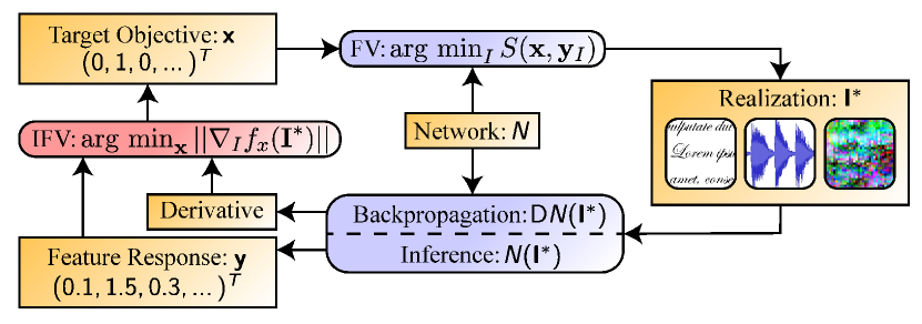
Figure 1: Interplay between Feature Visualization (FV) and Inverse Feature Visualization IFV (in red). Given an input ${\mathbf{I}^{*}}$ that is optimized via FV for a prescribed target objective $\mathbf{x}$, IFV recovers $\mathbf{x}$ solely from the network’s response to ${\mathbf{I}^{*}}$ and gradient information. If features and neurons of the network are not in 1:1/̄correspondence, this is ensured via an aggregation term $\operatorname{Agg}$—concatenated with the network function $N$—that maps activations to features. The function $f_{\mathbf{x}}$ is given by $I\mapsto S(\mathbf{x},\mathbf{y}_{I})$.

Unfortunately, solving Opt. (2) directly usually fails due to trivial solutions for $\mathbf{x}$. These occur at saddle or minimal points of $f_{\mathbf{x}}$, or are induced by nontrivial co/̄kernels of matrices that propagate when chaining Jacobian matrices to form $\nabla f_{\mathbf{x}}$. We introduce a method called Gradient based Inverse Feature Visualization (Grad/̄IFV) to address these limitations. Our key idea is to eliminate saddle points by introducing factors in $f_{\mathbf{x}}$ and intersecting the search space $\Omega$ with an appropriate subspace of $\mathbb{R}^{n_{f}}$. The consequential reformulation of Opt. (2) is solved by computing a singular value decomposition of a matrix derived from the gradient of the objective function $f_{\mathbf{x}}$.

While in this work we demonstrate that Grad/̄IFV can reproduce the target objective for which a given input was optimized, building upon this observation it then needs to be investigated whether Grad/̄IFV can be extended to arbitrary input. In this way, it may even become possible to control certain patterns in the inputs and ask for the specific features that are sensitive for them. This sheds light on the question whether it can be determined which patterns in the given inputs are relevant and which feature combinations of a network have learned these patterns, i.e., strive toward transfer learning. By inverting an input representing feature $\mathbf{x}$ in one network, the feature $\widetilde{\mathbf{x}}$ that is represented by this input in another network can be obtained. This can give rise to a feature-based comparison of learned representations, including insight into the relevance of patterns for successful network training.

2 Method

In this work, we consider FV objective functions provided by the Lucid library (Olah et al., 2017). For a thorough discussion of the use and interpretation of objective functions in the context of FV, let us refer to the recent work by Carter et al. (2019). The objective function $f_{\mathbf{x}}$ is a concatenation of three functions $N$, $\operatorname{Agg}$ and $S_{\mathbf{x}}$, where $N\colon\mathcal{I}\rightarrow\mathcal{A}$ represents the network and maps an input to activations that were tapped from the network, $\operatorname{Agg}\colon\mathcal{A}\rightarrow\mathbb{R}^{n_{f}}$ aggregates neuron activations into a feature response $\mathbf{y}$ of which component $i$ represents excitement of feature $i$ and $S_{\mathbf{x}}\colon\mathbb{R}^{n_{f}}\rightarrow\mathbb{R}$ is defined as $S_{\mathbf{x}}(\mathbf{y})=\mathbf{x}^{T}\mathbf{y}\cdot(\mathbf{x}^{T}\mathbf{y}/||\mathbf{y}||)^{k}$ with $k\in\mathbb{N}_{0}$. The set of allowed target objectives $\Omega$ is set to the $n_{f}D$/̄sphere containing feature directions, i.e. normalized linear combinations of features. The term $\mathbf{x}^{T}\mathbf{y}$ measures the length of the projection of $\mathbf{y}$ onto $\mathbf{x}$, and $\mathbf{x}^{T}\mathbf{y}/||\mathbf{y}||$ is the cosine similarity of $\mathbf{x}$ and $\mathbf{y}$.

If $N$ has an input domain $\mathcal{I}$ that is not a vector space $\mathbb{R}^{m}$, Opt. (2) is a constrained optimization problem for which a) common solvers such as gradient descent or Adam cannot be applied, and b) the necessary condition for optimality can be violated at the domain boundary $\partial\mathcal{I}$. These issues can be circumvented by means of a differentiable, surjective mapping $P\colon\mathbb{R}^{n_{p}}\rightarrow\mathcal{I}$, which parametrizes the input domain $\mathcal{I}$ by a real/̄valued vector space of dimension $n_{p}$. If such a $P$ is available, the constrained optimization problem $\operatorname*{arg\,min}_{I\in\mathcal{I}}f_{\mathbf{x}}(I)$ can be transformed to an unconstrained one over $n_{p}$ variables via $\operatorname*{arg\,min}_{v\in\mathbb{R}^{n_{p}}}(f_{\mathbf{x}}\circ P)(v)$.

In the following, if $I\in\mathcal{I}$ is an input configuration, we use $v_{I}$ to indicate a valid parameter vector that describes $I$, i.e., $P(v_{I})=I$. Furthermore, $P$, $N$, $\operatorname{Agg}$ are combined into a single function $\operatorname{\widetilde{N}}\mathrel{\mathop{\mathrel{\mathop{\mathchar 58\relax}}}}=\operatorname{Agg}\circ N\circ P$, which maps parameter vectors to feature responses. The feature response $\operatorname{\widetilde{N}}(v_{I})$ of $I$ is denoted by $\mathbf{y}_{I}$, and the Jacobian matrix $\operatorname{D\!}\operatorname{\widetilde{N}}(v_{I})$ is written as $\operatorname{D\!}\mathbf{y}_{I}$.

2.1 Reformulation of $\nabla f_{\mathbf{x}}$

Given the described family of objective functions, the gradient $\nabla f_{\mathbf{x}}$ can be computed. The chain rule allows us to write $\nabla(f_{\mathbf{x}}\circ P)(v_{I})=(k+1)q_{I}^{k}x^{T}Z_{k}(\mathbf{y}_{I})\operatorname{D\!}\mathbf{y}_{I}$, where $Z_{k}(\mathbf{y})=Z_{k}(\mathbf{y})^{T}\mathrel{\mathop{\mathrel{\mathop{\mathchar 58\relax}}}}=\mathit{Id}-k/(k+1)\overline{\mathbf{y}}\overline{\mathbf{y}}^{T}$, $\overline{\mathbf{y}}\mathrel{\mathop{\mathrel{\mathop{\mathchar 58\relax}}}}=\mathbf{y}/||\mathbf{y}||$, $q_{I}\mathrel{\mathop{\mathrel{\mathop{\mathchar 58\relax}}}}=\mathbf{x}^{T}\overline{\mathbf{y}_{I}}$ (see supp. material). The scalar factor $(k+1)q_{I}^{k}$ equals zero if $\mathbf{x}^{T}\mathbf{y}_{I}=0$. Depending on the parity of $k$, values of $\mathbf{y}_{I}$ with $\mathbf{x}^{T}\mathbf{y}_{I}=0$ either yield minimal or saddle points of $S_{\mathbf{x}}$. Since one is interested in maximizing $S_{\mathbf{x}}$, the factor can be safely dropped. Hence, if ${\mathbf{I}^{*}}$ is a local maximum for $f_{\mathbf{x}}$, this implies that $||\mathbf{x}^{T}Z_{k}(\mathbf{y}_{\mathbf{I}^{*}})\operatorname{D\!}\mathbf{y}_{\mathbf{I}^{*}}||=0$.

In practice, the investigated network may have linear relations that result in $\operatorname{D\!}\mathbf{y}_{I}$ and potentially $Z_{k}(\mathbf{y}_{I})\operatorname{D\!}\mathbf{y}_{I}$ having a nontrivial co/̄kernel that is similar for all $I\in\mathcal{I}$. For instance, dead neurons absorb gradients and introduce zero rows such that $e_{i}\in\bigcap_{I\in\mathcal{I}}\operatorname{coker}\operatorname{D\!}\mathbf{y}_{I}$ for some $i$. As a consequence, $e_{i}$ will always be a trivial solution to $||\mathbf{x}^{T}Z_{k}(\mathbf{y}_{\mathbf{I}^{*}})\operatorname{D\!}\mathbf{y}_{\mathbf{I}^{*}}||=0$, independently of the realization ${\mathbf{I}^{*}}$ and its target objective. Thus, we introduce an additional constraint filtering out trivial solutions. Instead of solving Opt. (2), it is then solved

$$\operatorname*{arg\,min}_{\mathbf{x}\in\Omega}||\mathbf{x}^{T}Z_{k}(\mathbf{y}_{I})\operatorname{D\!}\mathbf{y}_{I}||^{2}\quad\text{s.t.}\quad Z_{k}(\mathbf{y}_{I})\mathbf{x}\in C$$ (3)

Here, $C\subseteq\mathbb{R}^{n_{f}}$ denotes a freely selectable subspace not dependent on $I$, which we call critical space. By setting

$$C\mathrel{\mathop{\mathrel{\mathop{\mathchar 58\relax}}}}=\left(\bigcap_{I\in\mathcal{I}}\operatorname{coker}\operatorname{D\!}\mathbf{y}_{I}\right)^{\perp},$$ (4)

the previously described degeneracy can be avoided. Since the constraint is linear in $\mathbf{x}$, we can find a length preserving substitution $\mathbf{x}=U\sigma$ that reduces Opt. (3) to solving $\operatorname*{arg\,min}_{||\sigma||=1}||\sigma^{T}U^{T}Z_{k}(\mathbf{y}_{I})\operatorname{D\!}\mathbf{y}_{I}||^{2}$ (see supp. material). The solution (up to a sign) is given by the left/̄singular vector to the smallest singular value of $M\mathrel{\mathop{\mathrel{\mathop{\mathchar 58\relax}}}}=U^{T}Z_{k}(\mathbf{y}_{I})\operatorname{D\!}\mathbf{y}_{I}$. Thus, first a single forward and $n_{f}$ backward passes are run to determine $\mathbf{y}_{I}$ and $\operatorname{D\!}\mathbf{y}_{I}$. Then, $MM^{T}\in\mathbb{R}^{n_{f}\times n_{f}}$ is computed. The eigenvalue decomposition of $MM^{T}$ yields the desired left/̄singular vector of $M$.

2.2 Identifying the Critical Space

Since we do not make any assumptions about the architecture of $N$, the network’s state (i.e., weights, biases, etc.) cannot be used to deduce $C$. Instead, we sample $n$ random target objectives $\mathbf{x}_{i}$ ($i\in\{1,\dots,n\}$), compute realizations ${\mathbf{I_{i}}^{*}}$ by applying FV, and then try to approximate $C$ by investigating the matrices $\operatorname{D\!}\mathbf{y}^{(i)}$. We denote $\operatorname{D\!}\mathbf{y}_{\mathbf{I_{i}}^{*}}$ by $\operatorname{D\!}\mathbf{y}^{(i)}$ and $\mathbf{y}_{\mathbf{I_{i}}^{*}}$ by $\mathbf{y}^{(i)}$. In practice, the matrices $\operatorname{D\!}\mathbf{y}^{(i)}$ will not develop clear co/̄kernels, due to numerical inaccuracy, incomplete training runs, or stochastic optimization, just to mention a few reasons. Hence, special care has to be taken when designing an algorithm to determine $C$. Instead of searching for co/̄kernels, we search for a subspace $C$ of which its vector-matrix products with the sampled matrices $\operatorname{D\!}\mathbf{y}^{(i)}$ diminish, i.e., the spectral norm quotients $||C^{T}\operatorname{D\!}\mathbf{y}^{(i)}||_{2}/||\operatorname{D\!}\mathbf{y}^{(i)}||_{2}$ have to become small.

Algorithm 1 Co/̄kernel Approximation

  Input: Samples $\operatorname{D\!}\mathbf{y}^{(1)},\dots,\operatorname{D\!}\mathbf{y}^{(n)}$, threshold $\rho$

  for $i=1$ to $n$ do

     Compute $U\Sigma V^{T}=\operatorname{SVD}(\operatorname{D\!}\mathbf{y}^{(i)})$

     $S_{i}\leftarrow\operatorname{span}\{U_{\cdot,j}\mid\Sigma_{j,j}<\rho\cdot||\operatorname{D\!}\mathbf{y}^{(i)}||_{2}\}$

  end for

  $L\leftarrow\{(S_{1},1),\dots,(S_{n},1)\}$

  while $|L|>1$ do

     Remove $(U,w_{U})$, $(V,w_{V})$ from $L$

     Compute principal vectors $(p_{U}^{1},p_{V}^{1}),\dots,(p_{U}^{m},p_{V}^{m})$

     Drop all pairs with $\sphericalangle(p_{U}^{j},p_{V}^{j})>45^{\circ}$

     Interpolate $p_{I}^{j}\leftarrow\operatorname{SLERP}(p_{U}^{j},p_{V}^{j};w_{V}/(w_{U}+w_{V}))$

     $L\leftarrow L\cup\{(\operatorname{span}\{p_{I}^{j}\mid j\ \text{not dropped}\},w_{U}+w_{V})\}$

  end while

  return $U^{\perp}$ with $(U,w_{U})\in L$

Algorithm 1 approximates Eq. (4). First, the co/̄kernels are roughly approximated by computing a subspace of left/̄singular vectors with reasonable small singular values $<\rho\cdot||\operatorname{D\!}\mathbf{y}^{(i)}||_{2}$ for each sample. Afterwards, two subspaces at a time are merged until one is left over. The merging is implemented by computing the principal angles and vectors as suggested by Knyazev & Argentati (2002), dropping all vectors with principal angles of $45^{\circ}$ or higher and then applying spherical linear interpolation (SLERP) to each pair of corresponding left and right principal vectors. Thereby, the interpolation parameter is given by the ratio of subspaces that already have been merged into either of the two spaces to merge. The set of newly acquired vectors form a basis of the merged space. It can be interpreted as a roughly approximated intersection of two spaces, with the exact intersection being obtained when dropping all principal vectors with principal angles not exactly $0^{\circ}$. Note that the result of Algorithm 1 depends both on choices for the singular value threshold as well as the order in which subspaces are merged.

In a perfect world, solving Opt. (3) for a sample ${\mathbf{I_{i}}^{*}}$ would yield a projected target objective $\widetilde{\mathbf{x}}_{i}\in\Omega\cap Z_{k}(\mathbf{y}^{(i)})^{-1}C$ such that $Z_{k}(\mathbf{y}^{(i)})\widetilde{\mathbf{x}}_{i}$ points into the same direction as $Z_{k}(\mathbf{y}^{(i)})\mathbf{x}_{i}$ projected onto $C$. It is uniquely determined by normalizing $Z_{k}(\mathbf{y}^{(i)})^{-1}C_{M}C_{M}^{T}Z_{k}(\mathbf{y}^{(i)})\mathbf{x}_{i}$. This means that the realization’s target objective $\mathbf{x}_{i}$ can only be recovered modulo a shift in $(Z_{k}(\mathbf{y}^{(i)})^{-1}C)^{\perp}$ direction followed by a renormalization. One cannot expect to be any better since the objective function parametrization $\mathbf{x}\mapsto f_{\mathbf{x}}({\mathbf{I_{i}}^{*}})$ is (by construction of $C$) constant on $(Z_{k}(\mathbf{y}^{(i)})^{-1}C)^{\perp}$/̄shifts. In terms of maximum likelihood estimation, one still finds a solution for $\operatorname*{arg\,max}_{\mathbf{x}}f_{Y}(\mathbf{I};\mathbf{x})$. However, it may be another point on the plateau of the graph of $f_{Y}(\mathbf{I};\cdot)$ where the realization’s target objective one started with resides as well.

2.3 The Adversary - Aggregation

Common choices for $\operatorname{Agg}$  Olah et al. (2017) either average along the activations of all neurons associated with a feature, or pick a single representative activation—for instance the center pixel of a feature map. Both approaches have limitations. When aggregating over activations returned by a convolution filter such as a Sobel filter, except for border pixels, all contributions of pixels being convolved cancel out. Any filter would thus degenerate to a detector of color patches plus some border pattern. More general, aggregating along a dimension would eliminate the effect of a preceding linear operation in this dimension. When picking only a single neuron’s activation as representative, the realization returned by FV becomes sensitive to its receptive field, rendering realizations of different layers or network architectures incomparable. Although this does not pose an immediate issue for IFV itself, it counteracts our main motivation of using IFV techniques for network comparison later on.

To overcome these limitations, we propose to use a max/̄pooling operation followed by mean/̄aggregation. While the latter operation is independent of the receptive field, the former breaks linearities and allows us to still distinguish between different convolution filters. Note that a basic mean operation may also be sufficient if the activations returned by $N$ are generated by a rectified linear activation function (ReLU) or max/̄pooling operation. We suggest to always include operations breaking linearity in the aggregation process.

3 Results and Evaluation

In the following we analyze the accuracy of Grad/̄IFV and how the recovered target objectives differ from feature responses. FV is applied to three networks with different topology, size and application domains, to generate realizations for randomly sampled target objectives $\mathbf{x}_{i}$. Given these realizations, Opt. (3) is solved to yield the solutions ${\mathbf{\mathbf{x}_{i}}^{*}}$, which are then compared to the target objectives $\mathbf{x}_{i}$. We will subsequently call the solutions ${\mathbf{\mathbf{x}_{i}}^{*}}$ predicted objectives, since they are returned by Grad/̄IFV and are supposed to be an accurate estimate for the target objectives.

3.1 Network Architectures

GoogLeNet: GoogLeNet (Szegedy et al., 2015) builds upon stacked Inception modules, each of which takes the input of the previous layer, applies convolution filters with kernel sizes ($1\times 1$, $3\times 3$, and $5\times 5$), and concatenates all resulting feature maps into a single output vector. GoogLeNet has been trained for image classification, its input domain is given by $224\times 224$ RGB/̄images.

DenseNet: The DenseNet-BC architecture (Huang et al., 2017), with growth rate $k=12$, has been trained on the CIFAR-10 subset of the 80 million Tiny Images dataset (Torralba et al., 2008; Krizhevsky, 2009). Its input domain is given by $224\times 224$ RGB/̄images that are partitioned into 10 different classes. Three dense blocks are connected via convolution layers, followed by max pooling, form the core part of the network. Within a dense block, each layer takes the outputs of all preceding layers as inputs and processes them by applying a $1\times 1$/̄bottleneck convolution, batch normalization, ReLU activation, and finally a $3\times 3$/̄convolution. The output is passed to all subsequent layers of the dense block. In total, 0.8M weights are trained with weight decay by stochastic gradient descent with nesterov momentum. During training, images are flipped, padded with 4 pixels on each side, and cropped back to its original size with a random center.

SRNet: The fully convolutional SRNet (Sajjadi et al., 2018) has been modified and trained to upscale low resolution geometry images (normal and depth maps) of isosurfaces in scalar volume data by Weiss et al. (2019). The low resolution input size is set to $128\times 128$ pixels. Residual blocks of $3\times 3$ convolutions transform the input maps into a latent space representation, which is then upsampled, folded, and added as residual to bilinearly upscaled versions of the input. The input domain is given by a 2D normal field comprised of 3D vectors, a 2D depth map with values in the range $[0,1]$, and a 2D binary mask with values in $\{-1,1\}$ to indicate surface hits during rendering.

3.2 Feature Visualization

If not stated otherwise, the components of the objective function $f_{\mathbf{x}}$ used for FV are as follows: The network function $N$ applies the network up to the investigated layers (that is inception4c, dense3 etc.) and outputs their respective activations as a 3D-tensor with 2 spatial and 1 channel dimension. The aggregation operation $\operatorname{Agg}$ then applies 2D max pooling with kernel size $3\times 3$ and a stride of $1$ followed by taking the mean. Both operations are performed along the spatial dimension so that one ends up with a 1D vector of ,,channel activations” that act as our feature response. Here, each channel constitutes a separate feature. The feature response is combined with the target objective $\mathbf{x}$ as described in Sec. 2. The power $k$ of the cosine term is set to $2$. Last but not least, the used parametrization $P_{\text{rgb}}$ yields batches of RGB images clamped to values in $[0,1]$ by applying the sigmoid function to the unbounded space $\mathbb{R}^{H\times W\times 3}$, where $H$ and $W$ denote the respective input image dimensions for the investigated network.

The target objectives $\mathbf{x}$ with nonnegative entries are sampled from a vector distribution $X$ with uniform Hoyer sparseness measure (i.e. $\operatorname{hoyer}(X)\sim\mathcal{U}\{0,1\}$) (Hoyer, 2004). After sampling $\mathbf{x}$, we optimize for $\operatorname*{arg\,min}_{v\in\mathbb{R}^{n_{p}}}(f_{\mathbf{x}}\circ P)(v)$ by first applying Adam optimization (Kingma & Ba, 2014) followed by some steps of fine tuning with L/̄BFGS (Byrd et al., 1995). For DenseNet and SRNet, we run 800 steps of Adam and 300 steps of L/̄BFGS. To let GoogLeNet converge to an optimum, we run 3000 steps of Adam followed by 500 steps of L/̄BFGS.

3.3 Time Complexity & Performance

The runtime complexity of solving Opt. (3) and Algorithm 1 is $\mathcal{O}(\max(n_{p}n_{f}^{2},n_{f}^{3}))$ per sample. Runtime is dominated by singular value decompositions and multiplication of $n_{f}\times n_{f}$ and $n_{f}\times n_{p}$ matrices. The computation of $\operatorname{D\!}\mathbf{y}$ requires $n_{f}$ backward passes through the network, making it strongly dependent on the network architecture. Performance measurements are performed on a server architecture with 4x Intel Xeon Gold 6140 CPUs with 18 cores @ 2.30GHz each, and an NVIDIA GeForce GTX 1080 Ti graphics card with 11 GB VRAM. Timings are shown in Table 1. Note that the generation of realizations takes significantly longer due to the additional L/̄BFGS steps. Except for Algorithm 1, all computations are executed on the GPU.

3.4 The Simple Case

In the first experiment, the 512 filters in the inception4c layer of GoogLeNet, which we abbreviate by GN4c, are investigated. We sample 150 target objectives $\mathbf{x}_{i}$ as described above and add further 150 canonical vectors of sparsity measure 1. Then, FV is performed. For each resulting realization ${\mathbf{I_{i}}^{*}}$, a target objective ${\mathbf{x_{i}}^{*}}$ is predicted by solving Opt. (3), and then compared to $\mathbf{x}_{i}$ by measuring their angular distance in degrees, i.e., $180/\pi\cdot\min\{\cos^{-1}(-\mathbf{x}_{i}^{T}{\mathbf{x_{i}}^{*}}),\cos^{-1}(\mathbf{x}_{i}^{T}{\mathbf{x_{i}}^{*}})\}$. The elimination of trivial solutions in not required yet, hence we set $C=\mathbb{R}^{n_{f}}$.

Table 1: Timings for computing realizations via FV (${\mathbf{I_{i}}^{*}}$), back/̄propagation ($\operatorname{D\!}\mathbf{y}^{(i)}$), solving Opt. (3) (${\mathbf{x_{i}}^{*}}$) and re/̄optimization of ${\mathbf{I_{i}}^{*}}$ (re-opt.), for different number of input parameters ($n_{p}$) and features ($n_{f}$). All timings are in seconds per sample. Timings associated to IFV are in bold. Critical space computation for DN[4]cl takes $0.5$s on average per space. Batch sizes in FV are 8 for GN4c, 64 for DN[4]cl and DNde, and 32 for SRNet. Re/̄optimization always is performed with a batch size of 64. Solutions of Opt. (3) are computed for all samples at once, in a single batch.

Model	$n_{p}$	$n_{f}$	${\mathbf{I_{i}}^{*}}$	$\operatorname{D\!}\mathbf{y}^{(i)}$	${\mathbf{x_{i}}^{*}}$	re/̄opt.
GN4c	$224^{2}\cdot 3$	$512$	$17.3$	$\mathbf{0.7}$	$\mathbf{0.2}$	$0.7$
DN[4]cl	$32^{2}\cdot 3$	$10$	$2.1$	$\mathbf{0.0}$	$\mathbf{0.0}$	$0.7$
DNde	$32^{2}\cdot 3$	$342$	$2.0$	$\mathbf{0.3}$	$\mathbf{0.1}$	$0.7$
SRNet	$128^{2}\cdot 4$	$64$	$10.7$	$\mathbf{0.4}$	$\mathbf{0.0}$	$3.1$

The horizontal margin distribution in Fig. 2a shows the angular distances between the target objectives and either the predicted objectives ${\mathbf{x_{i}}^{*}}$, feature responses $\mathbf{y}^{(i)}$, or randomly sampled vectors. Note that whereas the angular distance between $\mathbf{x}_{i}$ and $\mathbf{y}^{(i)}$ is about $45^{\circ}$ (or a cosine similarity of $\approx 0.7$) with large variance, the predictions ${\mathbf{x_{i}}^{*}}$ show only a deviation of approx. $10^{\circ}$ ($\approx 0.98$ in terms of cosine similarity!) with very few outliers.

\begin{overpic}[width=140.92517pt,tics=10,trim=0.0pt 0.0pt 0.0pt 0.0pt,clip]{images/gnet_intro_coefplot} \end{overpic}

\begin{overpic}[width=140.92517pt,tics=10,trim=0.0pt 0.0pt 0.0pt 0.0pt,clip]{images/critical_space_coefplot} \end{overpic}

\begin{overpic}[width=140.92517pt,tics=10,trim=0.0pt 0.0pt 0.0pt 0.0pt,clip]{images/critical_space_ex4_coefplot} \end{overpic}

\begin{overpic}[width=140.92517pt,tics=10,trim=0.0pt 0.0pt 0.0pt 0.0pt,clip]{images/gnet_intro_jointplot} \put(0.0,2.0){{{\color[rgb]{0,0,0}\large(a)}}} \end{overpic}

\begin{overpic}[width=140.92517pt,tics=10,trim=0.0pt 0.0pt 0.0pt 0.0pt,clip]{images/critical_space_jointplot} \put(0.0,2.0){{{\color[rgb]{0,0,0}\large(b)}}} \end{overpic}

\begin{overpic}[width=140.92517pt,tics=10,trim=0.0pt 0.0pt 0.0pt 0.0pt,clip]{images/critical_space_ex4_jointplot} \put(0.0,2.0){{{\color[rgb]{0,0,0}\large(c)}}} \end{overpic}

Figure 2: (a) GoogLeNet, (b) DenseNet, (c) DenseNetEx4. (top) Values $\alpha_{1},\dots,\alpha_{10}$ indicating the mean contribution of $j$/̄th left/̄singular vectors to the target objectives, stacked in a bar chart in increasing order of $j$. Bars of missing values are too small for plotting. (bot (a)) Bivariate distribution of angular distances to the target objectives (horizontal axis) and SSIM indices (vertical axis) when re/̄optimizing w.r.t. predicted objectives, target objectives, feature responses or random feature objectives. (bot (b,c)) Trivariate distribution when re/̄optimizing w.r.t. predicted objectives for different critical spaces. Point size encodes the fraction of the target objective $\mathbf{x}_{i}$ that lives in the respective critical space, that is $||v||/(||v||+||w||)$ with $\mathbf{x}_{i}=v+w$, $v\in Z_{k}(\mathbf{y}^{(i)})^{-1}C$, $w\in(Z_{k}(\mathbf{y}^{(i)})^{-1}C)^{\perp}$. Triangles represent instable samples for which re/̄optimization with the target objective yields an SSIM index lower than $0.7$.

Next, it is verified that the realizations are optimal w.r.t. the predicted objective. To achieve this, a realization is re/̄optimized w.r.t. either $\mathbf{x}_{i}$, ${\mathbf{x_{i}}^{*}}$, $\mathbf{y}^{(i)}$, or a random objective with Adam for 500 steps. Finally, the SSIM index between the realization before and after optimizing is computed. SSIM is a perception/̄based model to measure the similarity of two images w.r.t. structural information (Zhou Wang et al., 2004).

The results are shown in Fig. 2a. High SSIM indices confirm that almost all realizations remain optima under the predicted objectives, yet there is clearly more change happening when re/̄optimizing for the feature response as objective. This observation confirms the rationale underlying the Deep/̄Dream process (Mordvintsev et al., 2015) that enhancing features changes the input significantly. In particular, in many cases re/̄optimizing for the feature response yields similar results to re/̄optimizing for a random vector.

Note that the SSIM index is strictly lower than one when re/̄optimizing for the target objective. This observation relates back to the Adam optimizer having an internal state that has to warm up first before Adam convergences. Hence, even when initializing Adam with an instable, local optimum, Adam may leave it and converge to a completely different one, lowering the SSIM index significantly.

3.5 Utilizing the Critical Space

Next, we investigate the ten neurons in the classification layer of DenseNet for two differently trained networks. Since aggregation along spatial dimensions becomes unnecessary in this case, we set $\operatorname{Agg}\equiv\mathit{Id}$. The second network is trained in a similar way than the first network described above, yet it never sees any training data for class 4. The classification layers of both networks are denoted by DNcl and DN4cl respectively. We sample 290 target objectives and add the ten canonical ones.

When predicting objectives and comparing them to the target objectives $\mathbf{x}_{i}$ as in the previous section, Grad/̄IFV fails. The experiment represented by blue dots in Fig. 2b,c show that the predicted objectives do not resemble the target objectives. To see how close the target objective is to be an optimal solution for Opt. (3), we decompose each $\mathbf{x}_{i}$ as follows: Let $v_{i,1},\dots,v_{i,n_{f}}$ be the left/̄singular vectors of $Z_{k}(\mathbf{y}^{(i)})\operatorname{D\!}\mathbf{y}^{(i)}$ with singular values $\sigma_{i,1}\leq\sigma_{i,2}\leq\dots\leq\sigma_{i,n_{f}}$. Then we determine coefficients $c_{i,j}$ such that $\mathbf{x}_{i}=\sum_{j}c_{i,j}v_{i,j}$. Finally, we average along all squared coefficients of the same order and obtain values $\alpha_{j}=\sum_{i=1}^{n}(c_{i,j}^{2}/n)$ that indicate how much the $j$/̄th left/̄singular vectors contribute to the $\mathbf{x}_{i}$s. Note that $c_{i,0}=\mathbf{x}_{i}^{T}{\mathbf{x_{i}}^{*}}$ and that $90(1-c_{i,0}^{2})$ is the polynomial of degree two approximating the angular distance between $\mathbf{x}_{i}$ and ${\mathbf{x_{i}}^{*}}$ with coincidence in $c_{i,0}^{2}\in[0,0.5,1]$.

Since Grad/̄IFV always predicts the left/̄singular vector of $Z_{k}(\mathbf{y})\operatorname{D\!}\mathbf{y}$ to the lowest singular value, it performs well when $\alpha_{1}\approx 1$ and $\alpha_{j}\approx 0$ for $j>1$. As seen in Fig. 2a, $\alpha_{1}\approx 1$ holds true for the scenario of Sec. 3.4. However, the horizontal bars of Fig. 2b,c indicate additional contributions indicated by significant values for $\alpha_{2}$ and $\alpha_{3}$, respectively. When further investigating left/̄singular vectors, we realized that all contributions of $\alpha_{1}$ (and $\alpha_{2}$ for DN4cl) relate back to the same span of left/̄singular vectors for all samples. We consider these vectors to be trivial solutions of Opt. (3), which we intend to sort out.

To obtain the trivial solutions and their complement, the critical space, the first 32 of the 300 Jacobian matrices $\operatorname{D\!}\mathbf{y}^{(i)}$ are passed to Algorithm 1. We apply a nested intervals technique to determine all values of $\rho\in(0,1)$ that yield critical spaces of different dimensions. For DNcl, a single 9/̄dimensional critical space $C_{1}$ is determined, of which the complement is spanned by (approximately) $(1,\cdots,1)^{T}\in\mathbb{R}^{10}$. The same critical space $C_{1}$ is retrieved for DN4cl, accompanied by a second one $C_{2}$ of 8 dimensions with its complement being spanned by $(1,\cdots,1)^{T}$ and $e_{4}$. Presumably, $(1,\cdots,1)^{T}$ arises as trivial solution because the network learned to exploit the softmax translation invariance in order to improve on a regularization term on its weights. Similarly, $e_{4}$ relates back to a dead neuron of a class the network of DN4cl never has seen.

The solutions ${\mathbf{x_{i}}^{*}}$ of Opt. (3) are computed by setting $C$ to either the full 10/̄dimensional ambient space, $C_{1}$, or $C_{2}$. We evaluate how closely the predicted objectives resemble the target objectives by projecting both onto $(Z_{k}(\mathbf{y}^{(i)})^{-1}C)^{T}$ and computing their angular distance. The distribution of angular distances, which is shown in the horizontal margin plots of Fig. 2b,c, indicate that Grad/̄IFV performs well for one particular critical space ($C_{1}$ for DNcl and $C_{2}$ for DN4cl). In practice, the correct one can be identified by running the described procedure for a set of known, i.e. sampled, target objectives $\mathbf{x}$, choosing the best performing critical space, and then solving Opt. (3) for realizations ${\mathbf{I_{i}}^{*}}$ with unknown target objective.

When applying re/̄optimization, Fig. 2b,c indicates that all samples with high angular distance to the target objective exhibit a low SSIM index. In particular, target objectives cannot be recovered accurately for samples where FV failed to find a stable optimum (marked by triangles in Fig. 2b,c). Further, there exists a cluster of (stable) samples for which the SSIM index is low although the prediction is accurate. All samples in the cluster have in common that a notable fraction of their corresponding target objectives is located in the subspace $(Z_{k}(\mathbf{y}^{(i)})^{-1}C)^{\perp}$, which we just factored out. This observation gives evidence that, in practice, the objective function parametrization $\mathbf{x}\mapsto f_{\mathbf{x}}$ is not entirely constant for $(Z_{k}(\mathbf{y}^{(i)})^{-1}C)^{\perp}$/̄shifts, as it would be if $C$ is chosen to be the exact union of co/̄kernels as expressed in Eq. (4). Thus, whenever we eliminate outliers by dropping all predicted objectives with a low SSIM value, we loose some relevant results as well.

3.6 Dropping the Cosine Term

When experimenting with different numbers of features $n_{f}$ and alternative aggregation functions, we observed that—as long as we keep the cosine term of the significance measure $S_{\mathbf{x}}$ with a power of $k=2$—Grad/̄IFV is quite resilient. When increasing the number of features or exchanging the aggregation function by averaging or picking as described in Sec. 2.3, we notice only slight increases in angular distances with prediction quality being similar to the results of Sec. 3.4. Except for the very few occasional outliers which can be filtered out by re/̄optimizing the input w.r.t. the predicted objective and investigating the SSIM index, the target objective is reliably recovered.

However, when running the experiments again with the cosine term dropped ($k=0$), predictions may become unreliable. When only considering the first $160$ convolution filters in the dense3 block of DenseNet, which we call DNde from now on, predicted objectives still perform significantly better than just estimating $\mathbf{x}_{i}$ via the feature response $\mathbf{y}^{(i)}$. The SSIM index obtained by re/̄optimization does not drop below $0.89$. For more features, prediction quality starts to degenerate quickly. When considering more than $288$ of the $342$ available filters in DNde, almost all angular distances between ${\mathbf{x_{i}}^{*}}$s and $\mathbf{x}_{i}$s are in the range from $70^{\circ}$ to $90^{\circ}$. When increasing the feature count in the inception4c layer of GoogLeNet (GN4c), degradation starts to set in for $96$ features and continues up to $256$. Beyond, most predicted objectives are perpendicular to the target objective.

As discussed in Sec. 3.5, the target objective can be expressed as a linear combination of singular vectors, to investigate by which margin Grad/̄IFV fails to extract the correct prediction. The resulting $\alpha_{j}$/̄values for different feature counts $n_{f}$ are depicted by stacked bars in Fig. 3. The prediction quality of Grad/̄IFV can be assessed via the height of the lowest bar, which shows the value of $\alpha_{1}$. High fragmentation of the bar charts suggests that target objectives cannot solely be recovered by setting up an appropriate critical space—at least not by one perpendicular to singular vectors of small singular values as returned by Algorithm 1.

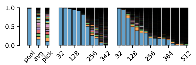
Figure 3: Values of $\alpha_{j}$ (i.e., mean contribution of $j$-th singular vectors, ordered by singular values, to target objectives) for different experiments with dropped cosine term, stacked in a bar chart in increasing order of $j$. Black indicates high fragmentation. Statistics for (left) $80$ filters in the dense3 block of DenseNet for different aggregation routines, (middle) $n_{f}$ filters of DNde, and (right) GNcl, where $n_{f}$ increases in steps of $32$.

Next, we consider the first $80$ filters of DNde and exchange the aggregation function. The coefficient histograms of Fig. 3 show that Grad/̄IFV fails to extract meaningful predictions for averaging- and picking/̄aggregations, although the results for max pooling followed by averaging are close to perfect.

Interestingly, when the experiments are conducted with $k=2$—i.e. with the cosine term—accurate predictions are obtained. In this case, FV has limited options in order to produce a visualization so that objectives pointing into perpendicular direction of $\mathbf{y}$ can be ignored during IFV. In Sec. 2.1, the matrix $Z_{k}(\mathbf{y})$ shrinks all vectors in the input’s feature response direction and thus makes them more likely to be the left/̄singular vector to the smallest singular value.

3.7 Different Parameterizations

We further investigate the influence of the parametrization $P$ on Grad/̄IFV. Therefore, we define the variables $v$ over which FV optimizes in Fourier space and perform spatial de/̄correlation (Olah et al., 2017), i.e., $P_{\text{fft}}$ is set to the inverse discrete fourier transform (iFFT) followed by sigmoid clamping. A parametrization favoring low frequencies can be obtained by scaling Fourier coefficients according to their frequency energies before applying iFFT, denoted by $P_{\text{ffte}}$. For each parametrization $P_{\text{rgb}}$, $P_{\text{fft}}$ and $P_{\text{ffte}}$, Grad/̄IFV is applied to GN4c and DNde. Although the image quality of the resulting realizations change notably (see Fig. 4), the quality of predicted objectives is not influenced. In particular, results do not suffer from low image quality of FV in case no regularizations such as transformation robustness are used.

Lastly, we analyze the SRNet for upscaling geometry images. We parameterize the normal map by coordinates $(\varphi,\theta)$, yet $\varphi$ is not bound to an interval length of $2\pi$ so that warping gradients at interval borders can be avoided. To ensure that the $z$/̄component is positive, we restrict $\theta$ to the interval $[-\pi/2,\pi/2]$ by applying a sigmoid function followed by an appropriate affine transformation. The depth map is clamped to $[0,1]$ with the sigmoid function. The binary mask is either hard/̄coded to be one or parameterized continuously in the interval $[-1,1]$. Note that we cannot properly represent the mask by a discrete set of values since this would turn the optimization problem of FV (Opt. (1)) into a mixed-integer programming problem.

When investigating the 64 filters of the 8th residual block of SRNet, Grad/̄IFV always recovers the 64 sampled target objectives accurately up to an angular distance of $5^{\circ}$. We even obtain reliable results with angular distances $<20^{\circ}$, when dropping the cosine term of the objective function.

4 Limitations & Future Work

One of our major goals is to identify convolution filters with similar feature visualizations along different networks. Under the assumption that feature visualizations carry semantic information about what a network learns, such an approach can eventually raise network comparison from mere signal analysis of activations to a semantic level. IFV enables selecting and visualizing a feature using one network first, and then inverting the resulting realization using a second network. This yields two features obeying the same visualization and, thus, representing the same semantic concept.

\begin{overpic}[width=212.47617pt,tics=10,trim=0.0pt 0.0pt 0.0pt 0.0pt,clip]{images/parametrization_gnet} \put(0.0,-0.2){{\color[rgb]{1,1,1}\rule{14.79541pt}{11.09654pt}}} \put(0.0,2.0){{{\color[rgb]{0,0,0}\large(a)}}} \end{overpic}

\begin{overpic}[width=212.47617pt,tics=10,trim=0.0pt 0.0pt 0.0pt 0.0pt,clip]{images/parametrization_dense} \put(0.0,-0.2){{\color[rgb]{1,1,1}\rule{15.36446pt}{11.09654pt}}} \put(0.0,2.0){{{\color[rgb]{0,0,0}\large(b)}}} \end{overpic}

Figure 4: Realizations returned by FV when parameterizing images through (top) $P_{\text{rgb}}$, (mid) $P_{\text{fft}}$ and (bot) $P_{\text{ffte}}$. Visualized features stem from (a) GoogLeNet and (b) DenseNet.

In real scenarios, however, a realization that is optimal for one network will not be so for another network. It might not even be close to an optimum as long as the sensitivity of the objective function to high frequencies and noise is not reduced. In particular, Grad/̄IFV relies on an input that is close to optimal, since a gradient’s magnitude, in general, cannot reflect how distant an input is to an optimal solution in the surrounding.

Therefore, in future work we will consider to widen the scope of objective functions to include arbitrary input priors (such as in Mahendran & Vedaldi (2015) or Nguyen et al. (2016)). Furthermore, we intend to integrate concepts that facilitate the processing of visualizations that are robust w.r.t. transformations (Olah et al., 2017). Both, input priors and transformation robustness, are key techniques to generate consistent and interpretable visualizations. By considering such techniques in IFV, we hope to achieve feature predictions that are less sensitive to network variations or input noise.

Upon resolving these issues, IFV can be used for network comparison, to analyze learned representations of networks trained on different datasets. Here it will be interesting to investigate which features are shared between two networks, and whether invariant operations on a network’s weight space such as permuting or rescaling neurons can be recovered.

5 Conclusion

We introduce the problem of identifying target objectives under which Feature Visualization (FV) yields a certain input, and propose a solution for certain types of FV objective functions. We demonstrate that the (possibly unknown) target objective can be accurately approximated by performing a singular value decomposition of a modified version of the network’s Jacobian matrix. In cases where the Jacobian matrix is ill/̄behaving, we identify problematic subspaces and factor them out to obtain accurate results modulo the reduction. In a number of experiments we investigate the accuracy by which the target objective is recovered, and whether the input remains stable under the predicted objective, i.e., the result truly is an inverse of FV. We observe that different choices for layer size, aggregation and objective functions can have a significant impact on the proposed technique. Finally, we envision future research directions towards feature/̄based comparison of learned representations—including assessment of the relevance of patterns for successful network training—and the use of Inverse Feature Visualization for network comparison.

References

- Bach et al. (2015) Bach, S., Binder, A., Montavon, G., Klauschen, F., Müller, K.-R., and Samek, W. On pixel-wise explanations for non-linear classifier decisions by layer-wise Relevance Propagation. PLOS ONE, 10(7):1–46, 07 2015. doi:10.1371/journal.pone.0130140.
- Byrd et al. (1995) Byrd, R. H., Lu, P., Nocedal, J., and Zhu, C. A Limited Memory Algorithm for Bound Constrained Optimization. SIAM Journal on Scientific Computing, 16(5):1190–1208, 1995. doi:10.1137/0916069.
- Carter et al. (2019) Carter, S., Armstrong, Z., Schubert, L., Johnson, I., and Olah, C. Activation Atlas. Distill, 2019. doi:10.23915/distill.00015. https://distill.pub/2019/activation-atlas.
- Erhan et al. (2009) Erhan, D., Bengio, Y., Courville, A., and Vincent, P. Visualizing higher-layer features of a deep network. University of Montreal, 1341(3):1, 2009.
- Hoyer (2004) Hoyer, P. O. Non-negative matrix factorization with sparseness constraints. Journal of machine learning research, 5(Nov):1457–1469, 2004.
- Huang et al. (2017) Huang, G., Liu, Z., v. d. Maaten, L., and Weinberger, K. Q. Densely connected convolutional networks. In 2017 IEEE Conference on Computer Vision and Pattern Recognition (CVPR), pp. 2261–2269, July 2017. doi:10.1109/CVPR.2017.243.
- Kingma & Ba (2014) Kingma, D. P. and Ba, J. Adam: A method for Stochastic Optimization, 2014. URL https://arxiv.org/abs/1412.6980. arXiv: 1412.6980 [cs.LG].
- Knyazev & Argentati (2002) Knyazev, A. V. and Argentati, M. E. Principal angles between subspaces in an A-based scalar product: Algorithms and perturbation estimates. SIAM Journal on Scientific Computing, 23(6):2008–2040, 2002. doi:10.1137/S1064827500377332.
- Krizhevsky (2009) Krizhevsky, A. Learning multiple layers of features from Tiny Images. Technical report, University of Toronto, 2009.
- Li et al. (2015) Li, Y., Yosinski, J., Clune, J., Lipson, H., and Hopcroft, J. Convergent Learning: Do different neural Networks learn the same representations? In Storcheus, D., Rostamizadeh, A., and Kumar, S. (eds.), Proceedings of the 1st International Workshop on Feature Extraction: Modern Questions and Challenges at NIPS 2015, volume 44 of Proceedings of Machine Learning Research, pp. 196–212, Montreal, Canada, 11 Dec 2015. PMLR.
- Mahendran & Vedaldi (2015) Mahendran, A. and Vedaldi, A. Understanding deep image representations by inverting them. In 2015 IEEE Conference on Computer Vision and Pattern Recognition (CVPR), pp. 5188–5196, June 2015. doi:10.1109/CVPR.2015.7299155.
- Mordvintsev et al. (2015) Mordvintsev, A., Olah, C., and Tyka, M. Inceptionism: Going deeper into neural networks, 2015. URL https://ai.googleblog.com/2015/06/inceptionism-going-deeper-into-neural.html.
- Nguyen et al. (2015) Nguyen, A., Yosinski, J., and Clune, J. Deep neural networks are easily fooled: High confidence predictions for unrecognizable images. In 2015 IEEE Conference on Computer Vision and Pattern Recognition (CVPR), pp. 427–436, June 2015. doi:10.1109/CVPR.2015.7298640.
- Nguyen et al. (2016) Nguyen, A., Dosovitskiy, A., Yosinski, J., Brox, T., and Clune, J. Synthesizing the preferred inputs for neurons in neural networks via Deep Generator Networks. In Lee, D. D., Sugiyama, M., Luxburg, U. V., Guyon, I., and Garnett, R. (eds.), Advances in Neural Information Processing Systems 29, pp. 3387–3395. Curran Associates, Inc., 2016.
- Nguyen et al. (2019) Nguyen, A., Yosinski, J., and Clune, J. Understanding neural networks via Feature Visualization: A survey, pp. 55–76. Springer International Publishing, Cham, 2019. ISBN 978-3-030-28954-6. doi:10.1007/978-3-030-28954-6_4.
- Olah et al. (2017) Olah, C., Mordvintsev, A., and Schubert, L. Feature Visualization. Distill, 2017. doi:10.23915/distill.00007. https://distill.pub/2017/feature-visualization.
- Olah et al. (2018) Olah, C., Satyanarayan, A., Johnson, I., Carter, S., Schubert, L., Ye, K., and Mordvintsev, A. The Building Blocks of Interpretability. Distill, 2018. doi:10.23915/distill.00010. https://distill.pub/2018/building-blocks.
- Raghu et al. (2017) Raghu, M., Gilmer, J., Yosinski, J., and Sohl-Dickstein, J. SVCCA: Singular Vector Canonical Correlation Analysis for Deep Learning Dynamics and Interpretability. In Guyon, I., Luxburg, U. V., Bengio, S., Wallach, H., Fergus, R., Vishwanathan, S., and Garnett, R. (eds.), Advances in Neural Information Processing Systems 30, pp. 6076–6085. Curran Associates, Inc., 2017.
- Sajjadi et al. (2018) Sajjadi, M. S. M., Vemulapalli, R., and Brown, M. Frame-Recurrent Video Super-Resolution. In 2018 IEEE/CVF Conference on Computer Vision and Pattern Recognition, pp. 6626–6634, June 2018. doi:10.1109/CVPR.2018.00693.
- Simonyan et al. (2013) Simonyan, K., Vedaldi, A., and Zisserman, A. Deep inside Convolutional Networks: Visualising Image Classification Models and Saliency Maps, 2013. URL https://arxiv.org/abs/1312.6034. arXiv: 1312.6034 [cs.CV].
- Szegedy et al. (2013) Szegedy, C., Zaremba, W., Sutskever, I., Bruna, J., Erhan, D., Goodfellow, I., and Fergus, R. Intriguing properties of neural networks, 2013. URL https://arxiv.org/abs/1312.6199. arXiv: 1312.6199 [cs.CV].
- Szegedy et al. (2015) Szegedy, C., Liu, W., Jia, Y., Sermanet, P., Reed, S., Anguelov, D., Erhan, D., Vanhoucke, V., and Rabinovich, A. Going deeper with convolutions. In Proceedings of the IEEE conference on computer vision and pattern recognition, pp. 1–9, 2015.
- Torralba et al. (2008) Torralba, A., Fergus, R., and Freeman, W. T. 80 Million Tiny Images: A large data set for nonparametric object and scene recognition. IEEE Transactions on Pattern Analysis and Machine Intelligence, 30(11):1958–1970, Nov 2008. ISSN 1939-3539. doi:10.1109/TPAMI.2008.128.
- Wang et al. (2018) Wang, L., Hu, L., Gu, J., Hu, Z., Wu, Y., He, K., and Hopcroft, J. Towards understanding Learning Representations: To what extent do different neural networks learn the same representation. In Bengio, S., Wallach, H., Larochelle, H., Grauman, K., Cesa-Bianchi, N., and Garnett, R. (eds.), Advances in Neural Information Processing Systems 31, pp. 9584–9593. Curran Associates, Inc., 2018.
- Weiss et al. (2019) Weiss, S., Chu, M., Thuerey, N., and Westermann, R. Volumetric Isosurface Rendering with Deep Learning-based super-resolution. IEEE Transactions on Visualization and Computer Graphics, 2019. ISSN 2160-9306. doi:10.1109/TVCG.2019.2956697.
- Zhou Wang et al. (2004) Zhou Wang, Bovik, A. C., Sheikh, H. R., and Simoncelli, E. P. Image Quality Assessment: From error visibility to Structural Similarity. IEEE Transactions on Image Processing, 13(4):600–612, April 2004. ISSN 1057-7149. doi:10.1109/TIP.2003.819861.