Optimal universal programming of unitary gates

Abstract

A universal quantum processor is a device that takes as input a (quantum) program, containing an encoding of an arbitrary unitary gate, and a (quantum) data register, on which the encoded gate is applied. While no perfect universal quantum processor can exist, approximate processors have been proposed in the past two decades. A fundamental open question is how the size of the smallest quantum program scales with the approximation error. Here we answer the question, by proving a bound on the size of the program and designing a concrete protocol that attains the bound in the asymptotic limit. Our result is based on a connection between optimal programming and the Heisenberg limit of quantum metrology, and establishes an asymptotic equivalence between the tasks of programming, learning, and estimating unitary gates.

Introduction. A universal quantum processor is the desideratum of quantum computing. Ideally, one would hope to realise quantum computing in the same way as its classical counterpart, i.e., by inserting data and programs, both in the form of quantum states, into a universal quantum computer. However, the no-programming theorem Nielsen and Chuang (1997) asserts that any universal quantum processor must be approximate, or have a non-zero probability of failure Nielsen and Chuang (1997); Hillery et al. (2002); Sedlák et al. (2019).

It has been shown that approximate universal processors with a finite-size program register do exist Nielsen and Chuang (1997); Kim et al. (2001); Hillery et al. (2001); Vidal et al. (2002); Brazier et al. (2005); Ishizaka and Hiroshima (2008); Kubicki et al. (2019). There one of the most important questions is to determine the cost-accuracy tradeoff or, more specifically, how the program cost, i.e., the number $c_{\rm P}$ of qubits required to store the optimal program, scales with the desired accuracy of implementation, quantified by an approximation error $\epsilon$.

Over the past two decades, many efforts have been dedicated to finding the optimal approximate universal processor Kim et al. (2001); Hillery et al. (2001); Ishizaka and Hiroshima (2008); Kubicki et al. (2019) (see also Table 1). The state-of-the-art result, Kubicki et al. (2019), asserts that the optimal program cost $c_{\rm P}$ for a $d$-dimensional unitary quantum gate lies between $c_{\rm low}:=[(1-\epsilon)K]d-(2/3)\log d$ qubits and $c_{\rm upp}:=d^{2}\log\left(K/\epsilon\right)$ qubits, where $K$ is a universal constant. Despite all efforts, the precise value for $c_{\rm P}$ remained largely unknown — especially in the small error regime, where the ratio $c_{\rm upp}/c_{\rm low}$ diverges.

In this Letter, we close this gap by identifying the optimal scaling of the program cost with the accuracy and therefore solving a long-standing open problem of optimal quantum programming. Specifically, our program cost scales as $[(d^{2}-1)/2]\log\left(1/\epsilon\right)$ in the small $\epsilon$ regime, which reduces the cost of the best existing protocol (see $c_{\rm upp}$ above) by half. The optimal scaling is achieved with a gate learning protocol, where the program is prepared by sending a quantum state through $n$ instances of the gate to learn it Bisio et al. (2010). The gate information is later read out by measuring the program. Our protocol achieves a diamond norm error scaling of $1/n^{2}$ – well-known as the Heisenberg limit of quantum metrology Bužek et al. (1999); Chiribella et al. (2004); Bagan et al. (2004); Hayashi (2006). We thus prove the asymptotic equivalence of quantum gate programming, metrology, and learning.

	Upper bounds	Lower bounds
Previous works	$d^{2}\log\left(K/\epsilon\right)$ Kubicki et al. (2019)   $4d^{2}\log d/\epsilon^{2}$ Ishizaka and Hiroshima (2008); Beigi and König (2011); Christandl et al. (2018)	$[(1-\epsilon)K]d-(2/3)\log d$ Kubicki et al. (2019)    $\log\left(d^{2}/\epsilon\right)$ Majenz (2017)     $\left(\frac{d+1}{2}\right)\log\left(1/d\right)+\left(\frac{d-1}{2}\right)\log\left(1/\epsilon\right)$ Pérez-García (2006)
This work	$\left(\frac{d^{2}-1}{2}\right)\log\left(\Theta(d^{2})/\epsilon\right)$	$\alpha\log\left(\Theta(d^{-4})/\epsilon\right)$ for any $\alpha<(d^{2}-1)/2$ and sufficiently small $\epsilon$

Table 1: Comparison of bounds on universal quantum gate programming. In the table we compare our results on the programming cost with the best previous results (summarised from Table I of Ref. Kubicki et al. (2019)). In the vanishing error regime $\epsilon\to 0$, both our lower bound and our upper bound are tighter than all previous results, for the first time closing the gap between the lower and upper bound in this regime. The cost is defined as the number of qubits in the program and the error is evaluated in terms of the diamond norm (2). $K$ denotes a universal constant.

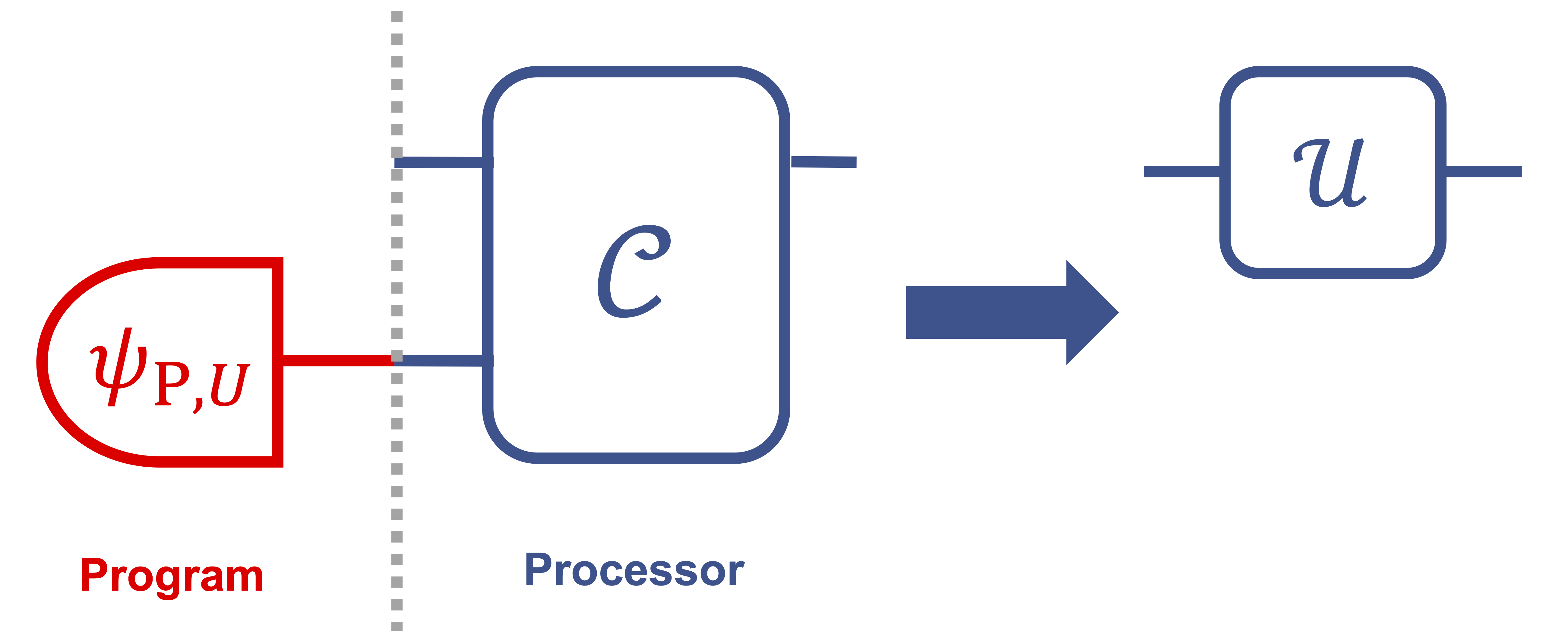
Figure 1: An approximate universal quantum processor. An approximate universal quantum processor executes a unitary gate $U$ on a system. It works by plugging a quantum state – the program for $U$ – into the processor, which performs a quantum channel $\mathcal{C}$ that approximates $U$ on the system.

Preliminaries. We consider programming unitary gates of a system with a $d$-dimensional Hilbert space $\mathcal{H}$. The gates, up to an irrelevant global phase, form the special unitary group $\mathsf{SU(d)}$. For a pure state $|\psi\rangle$, we abbreviate its density matrix $|\psi\rangle\langle\psi|$ by $\psi$. Similarity, $\mathcal{U}(\cdot):=U(\cdot)U^{\dagger}$ denotes a unitary channel.

We will use the big-$\Omega$ notation, the big-$O$ notation, and the big-$\Theta$ notation to characterise the asymptotic behaviour of functions. For two non-negative functions $f(n)$ and $g(n)$, we write $f(n)=\Omega(g(n))$ if there exists a constant $c_{1}>0$ so that $f(n)\geq c_{1}\,g(n)$ for large enough $n$, $f(n)=O(g(n))$ if there exists a constant $c_{2}>0$ so that $f(n)\leq c_{2}g(n)$ for large enough $n$, and $f(n)=\Theta(g(n))$ if $f(n)=\Omega(g(n))$ and $f(n)=O(g(n))$. We will also abbreviate $\log_{2}$ by $\log$.

Approximate universal processors. A universal quantum processor consists of two key elements: a family of programs $\{\psi_{{\rm P},U}\}_{U\in\mathsf{SU(d)}}$, which are quantum states in $\mathcal{H}_{\rm P}$, and the action of the processor $\mathcal{C}$, which is a quantum channel (i.e. a completely positive trace-preserving linear map) acting on the composite Hilbert space $\mathcal{H}_{\rm S}\otimes\mathcal{H}_{\rm P}$ of the system and the program. Notice that all information on $U$ should come from the program, and $\mathcal{C}$ must be independent of $U$. The program cost $c_{\rm P}$ is defined as $\log_{2}d_{\rm P}$, with the program dimension $d_{\rm P}$ being the dimension of $\mathsf{Supp}\{\psi_{{\rm P},U}\}_{U\in\mathsf{SU(d)}}$.

As shown in Figure 1, to run any arbitrary unitary $U$ on the system, one selects the corresponding program $\psi_{{\rm P},U}$ and plugs it into the processor, resulting in the following channel on the system:

$$\mathcal{E}_{U}(\cdot):=\operatorname{Tr}_{\rm P}\left[\mathcal{C}(\cdot\otimes\psi_{{\rm P},U})\right].$$ (1)

A pair $(\mathcal{C},\{\psi_{{\rm P},U}\}_{U\in\mathsf{SU(d)}})$ is called a $\epsilon$-universal processor, if

$$\frac{1}{2}\left\|\mathcal{U}-\mathcal{E}_{U}\right\|_{\diamond}\leq\epsilon\quad\forall\,U\in\mathsf{SU(d)}.$$ (2)

Here $\|\cdot\|_{\diamond}$ denotes the diamond norm Kitaev (1997), which equals the maximum trace distance between the outputs of the two channels, maximized over all input states and over all possible reference systems.

The no-programming theorem Nielsen and Chuang (1997) rules out perfect (i.e. $\epsilon=0$) universal processors with finite cost $c_{\rm P}<\infty$. This impossibility result raised the question: “Given a desired accuracy $1/\epsilon$, how big does the program need to be?” This question can of course be subdivided into two, namely to find upper and lower bounds on the program cost $c_{\rm P}$. We summarise the best known results in Table 1. Here we are providing both a new lower and a new upper bound, which match in terms of their asymptotic dependence on $1/\epsilon$.

Lower bound on the program cost. We first establish a lower bound on the program cost. For this purpose, we exploit an alternative proof of the no-programming theorem, originally developed in the framework of general probabilistic theories Chiribella et al. (2010). The idea is that the exact implementation of a unitary gate requires the channel $\mathcal{C}$ to leave the system and the program uncorrelated. Using this fact, the program can be recycled, thereby generating multiple copies of the desired unitary gate. The approximate version of this argument was first used by us to determine the energy requirement of quantum processors Chiribella et al. (2019) and is further exploited here.

To approximate a unitary quantum gate $U$ with good precision, there should be almost no correlation between the system and the program after we apply $\mathcal{C}$. This means that the complementary channel of $\mathcal{E}_{U}$, defined as $\overline{\mathcal{E}}_{\rho_{\rm S}}(\cdot):=\operatorname{Tr}_{\rm S}\left[\mathcal{C}\left(\rho_{\rm S}\otimes(\cdot)\right)\right]$, is almost independent of $\rho_{\rm S}$. It further suggests that, instead of discarding the program after one usage, we can recycle it: We can invert the action of $\overline{\mathcal{E}}_{\rho_{\rm S}}$ on the program state by a $(\rho_{\rm S})$-independent operation and get back the original program. The program can be further used, generating multiple uses of $U$ at the cost of an increased approximation error. Notice that the argument does not hold for noisy or classical processes. For instance, using a controlled unitary $|0\rangle\langle 0|\otimes I+|1\rangle\langle 1|\otimes\sigma_{z}$ and an ancillary qubit $(1/\sqrt{2})(|0\rangle+|1\rangle)$ one can (perfectly) implement the channel $\rho\to(1/2)(\rho+\sigma_{z}\rho\sigma_{z})$. However, the system and the ancillary qubit become strongly correlated after the implementation.

By the above argument, we can show (see Appendix for details) that an $\epsilon$-universal processor for a single use of $U$ can be turned into a $(4m\sqrt{2\epsilon})$-universal processor for $m$ uses of $U$ for any $m\geq 1$. This requires the original program to contain enough information for programming up to $1/\sqrt{\epsilon}$ uses of $U$. This fact, in turn, implies a bound on its minimum information content and therefore its size. This ultimately leads to the following theorem, which can be regarded as a quantitative version of the no-programming theorem Nielsen and Chuang (1997):

Theorem 1 (Approximate no-programming theorem).

Consider any $\epsilon$-universal processor with program cost $c_{\rm P}$. For any ($\epsilon$-independent) parameter $\delta>0$, the program cost is lower bounded as

$$c_{\rm P} \geq(1-\delta-4\sqrt{2\epsilon})(d^{2}-1)\log\left(\frac{\delta}{4\sqrt{2\epsilon}(d^{2}-1)}\right)-1.$$ (3)

This immediately implies the expression for the lower bound stated in Table 1. The key message from the above theorem is that, for any $\alpha<(d^{2}-1)/2$, the program dimension $d_{\rm P}=2^{c_{\rm P}}$ satisfies

$$d_{\rm P} =\Omega\left(1/\epsilon^{\alpha}\right)$$ (4)

Taking $\epsilon\to 0$ in Eq. (4), one gets $d_{\rm P}\to\infty$, recovering the original no-programming theorem Nielsen and Chuang (1997).

Optimal approximate universal processor. Next we construct an approximate universal processor that achieves the bound in Theorem 1. Our processor works in a measure-and-operate (MO) fashion, as illustrated in Figure 2. It measures the input program $\psi_{{\rm P},U}$ with a suitable POVM $\{\operatorname{d}\hat{U}\,M_{\hat{U}}\}_{\hat{U}\in\mathsf{SU(d)}}$, where $\operatorname{d}\hat{U}$ is the Haar measure. The measurement yields an estimate $\hat{U}$ of the gate $U$, and the processor performs the corresponding gate on the system. Explicitly, our optimal processor obeys the following procedure:

Protocol 1 A MO universal processor.

1:(Generating the program.)
Apply $U^{\otimes n}$ to a suitable quantum state $|\psi_{{\rm P}}\rangle$.

2:Measure $|\psi_{{\rm P},U}\rangle:=U^{\otimes n}|\psi_{{\rm P}}\rangle$ with $\{\operatorname{d}\hat{U}\,M_{\hat{U}}\}_{\hat{U}\in\mathsf{SU(d)}}$.

3:Apply $\hat{U}$ to the state of the system, where $\hat{U}$ is the measurement outcome.

Figure 2: A learning protocol for unitary gates. In the learning phase, a probe state $\psi_{\rm P}$, possibly entangled with a reference system, is prepared. It is then sent through $n$ parallel instances of $U$, resulting in a program $\psi_{{\rm P},U}$. The program is later measured, and the gate corresponding to the measurement outcome $\hat{U}$ is performed on the system.

The program in Protocol 1 is prepared by applying $n$ parallel uses of $U$ on a quantum state (called the probe state). The performance of this processor is then determined jointly by the choice of the probe state and the choice of the POVM $\{\operatorname{d}\hat{U}\,M_{\hat{U}}\}_{\hat{U}\in\mathsf{SU(d)}}$. It is known from quantum metrology Chiribella et al. (2004); Bagan et al. (2004); Kahn (2007) that the performance of the measurement is optimised using non-product probe states and POVMs. In Appendix, we identify a probe state and a POVM which, when incorporated into Protocol 1, yields an optimal processor asymptotically achieving the $({(d^{2}-1)/2})\log(1/\epsilon)$ scaling bound of Theorem 1.

Theorem 2.

Consider the estimation of an unknown unitary gate on a $d$-dimensional quantum system. When $n\geq 2d(d-1)$ uses of the gate are available, the diamond norm error for the optimal estimation is bounded as

$$\epsilon \leq 2\left(\frac{\pi(d-1)^{2}(3d-2)}{d\cdot n}\right)^{2}.$$ (5)

The probe state has dimension bounded as

$$d_{\rm P}\leq\left(\frac{9n}{3d-2}\right)^{d^{2}-1}.$$ (6)

Ref. Kahn (2007) showed that the estimation of an arbitrary $d$-dimensional unitary given $n$ uses can be done with an error scaling $1/n^{2}$. The error was measured by the entanglement gate infidelity, which is upper bounded by $1-(1-\epsilon)^{2}$. Theorem 2 refines this result by not only achieving the $1/n^{2}$ scaling but also identifying an explicit expression of the constant of proportionality. In addition, our result holds for the more stringent error criterion $\epsilon$, i.e., the diamond norm error, and we also determine how the probe state dimension scales with $n$.

Combining Eq. (5) with Eq. (6), we get:

Corollary 1.

The program cost $c_{\rm P}$ of Protocol 1 is upper bounded as

$$c_{\rm P}\leq\left(\frac{d^{2}-1}{2}\right)\log\left(\frac{162\pi^{2}(d-1)^{4}}{d^{2}\cdot\epsilon}\right).$$ (7)

It is obvious from the above corollary that

$$c_{\rm P}\leq\left(\frac{d^{2}-1}{2}\right)\log\left(\frac{162\pi^{2}d^{2}}{\epsilon}\right),$$ (8)

which matches Table 1 and achieves a quadratic reduction compared to known results.

Asymptotic equivalence of programming, metrology, and learning. From the previous discussion, we can see that an optimal way of programming a unitary is actually to let the processor learn and memorize it (see Figure 2). The task of learning a unitary $U$ from $n$ instances Gammelmark and Mølmer (2009); Bisio et al. (2010); Mo and Chiribella (2019) consists of a learning phase and an execution (or testing) phase. In the learning phase, the protocol makes $n$ (not necessarily parallel) queries to $U$. In the execution phase, the protocol emulates the learned unitary on an arbitrary input state. Notice that the execution phase happens after the learning phase, thus the protocol should be able to store the information of $U$.

A learning protocol induces a programmable processor in the sense that the learning phase can be used to generate a program. Nevertheless, one should keep in mind that learning and programming are not equivalent. Indeed, in the task of programming, the program does not have to be generated by learning, i.e., by applying multiple instances of $U$ on a quantum state. As learning has this additional constraint, its resource requirement is at least as stringent as that of programming. Therefore, since Protocol 1 is an optimal processor, it is also an optimal learning protocol. The performance of optimal learning given $n$ instances is thus given by Theorem 1, achieved by unitary gate metrology. In summary, for finite dimensional quantum gates, the performances of programming, metrology and learning are asymptotically equal:

$${\rm programming\approx metrology\approx learning.}$$

Quantum versus classical advantage. One may wonder if it is possible to simply use a classical program, e.g., to write down the description of the gate on a tape. Here we show, via a simple example, that our Protocol 1, which uses a quantum program, beats the best processor that uses classical programs in scaling.

Let us consider the case of programming a phase gate $U_{\theta}=|0\rangle\langle 0|+e^{-i\theta}|1\rangle\langle 1|$, where $\theta\in[0,2\pi)$ is the (unknown) phase, for it allows for explicit calculations. Fixing the program dimension $d_{\rm P}:=2^{c_{\rm P}}$, the best classical strategy is nothing but dividing the range $[0,2\pi)$ into $d_{\rm P}$ equal-width intervals. The tag of the interval that contains $\theta$ is used as the program, and the processor runs $U_{\hat{\theta}}$ with $\hat{\theta}$ being the middle point of the interval. Since $\max|\hat{\theta}-\theta|=\pi/d_{\rm P}$, the error of this approach is $\epsilon_{\rm classical}=\sqrt{(1-\cos(\pi/d_{\rm P}))/2}\simeq\pi/(2d_{\rm P})$, which is inversely proportional to the program dimension.

In contrast, we can employ our Protocol 1, where we use the sine state Bužek et al. (1999)

$$|\psi\rangle=\sqrt{\frac{2}{d_{\rm P}}}\sum_{m=0}^{d_{\rm P}-1}\sin\frac{\pi(m+1/2)}{d_{\rm P}}|m\rangle.$$ (9)

as the probe state and the covariant POVM $\left\{\frac{\operatorname{d}\hat{\theta}}{2\pi}|\eta_{\hat{\theta}}\rangle\langle\eta_{\hat{\theta}}|:|\eta_{\hat{\theta}}\rangle:=\sum_{m=0}^{d_{\rm P}-1}e^{-im\hat{\theta}}|m\rangle\right\}_{\hat{\theta}}$ as the measurement. The error can be evaluated as

$$\epsilon_{\rm quantum}\simeq\frac{\pi^{2}}{2d_{\rm P}^{2}},$$ (10)

which is inversely proportional to the square of the program dimension. In other words, the program dimension of a processor with classical programs is quadratically larger than that of our quantum processor. In the more complex case of programming a $d$-dimensional unitary gate, the classical strategy is to construct an $\epsilon$-mesh of the unitary gates, which was employed by Ref. Kubicki et al. (2019). The program cost was given in Table 1 as $d^{2}\log(K/\epsilon)$, higher than twice the cost of our quantum strategy in the small $\epsilon$ regime. This proves the claimed quantum-over-classical advantage in programming.

Conclusion and further discussions. We identified the optimal scaling of the program cost with accuracy in a universal quantum processor. The optimal scaling can be achieved with a measure-and-operate learning protocol. With this finding, we showed the asymptotic equivalence between programming, metrology, and learning.

In this work, we determined the optimal dependence of the program size on the accuracy parameter $\epsilon$. An interesting extension would be to determine the optimal scaling with the dimension of the target system $d$. Moreover, the task we focused on is universal programming, which requires the processor to work well for every gate of a certain dimension. It is natural to expect that a smaller set of gates would lead to a smaller program cost. Observe from Eq. (8) that the prefactor $(d^{2}-1)/2$ is exactly one half the number of real parameters determining a qudit unitary gate (up to a global phase). We therefore conjecture a general formula, valid for parametric families of quantum gates with a continuous dependence on $\nu$ real parameters:

$$c_{\rm P}\sim\left(\frac{\nu}{2}\right)\log\left(\frac{C_{\nu,d}}{\epsilon}\right),$$ (11)

where $C_{\nu,d}$ is a parameter, possibly dependent on $\nu$ and $d$ but independent of $\epsilon$.

Another key reason for making this conjecture is that the ultimate performances of quantum information processing tasks share similar forms in the asymptotic limit of “many copies”. In particular, one can consider the compression of identically prepared quantum systems, e.g. states of the form $\rho^{\otimes n}$ with $\rho$ unknown and $n$ being large. It turns out that the minimum cost of the memory, when requiring the error to be vanishing for large $n$, is $(\nu/2)\log n$ (qu)bits in the leading order Plesch and Bužek (2010); Rozema et al. (2014); Chiribella et al. (2015); Yang et al. (2016a, b, 2018). Here $\nu$, the number of variable real parameters, appears again. Further pursuit in this direction could lead to the discovery of a universality rule, which governs the behaviour of optimal quantum devices in the limit of macroscopically many copies.

Appendix A Proof of Theorem 1

Consider any $\epsilon$-universal processor $(\mathcal{C},\{\psi_{{\rm P},U}\})$. We prove Theorem 1 of the main text, which is a lower bound on the dimension $d_{\rm P}$ of the program, i.e. the dimension of $\mathsf{Supp}\{\psi_{{\rm P},U}\}$.

We first show that programming one use of $U$ with error $\epsilon$ requires the same amount of information as programming $m$ uses of $U$ with error $4m\sqrt{2\epsilon}$ for any $m\geq 1$. Note that the proof here extends that of (Chiribella et al., 2019, Corollary 2). First, we define the worst-case input (or minimum) fidelity between two arbitrary quantum channels $\mathcal{A}$ and $\mathcal{B}$, defined as Nielsen and Chuang (2000)

$$F_{\rm wc}(\mathcal{A},\mathcal{B}):=\inf_{\Psi}F\left((\mathcal{A}\otimes\mathcal{I}_{\rm R})(\Psi),(\mathcal{B}\otimes\mathcal{I}_{\rm R})(\Psi)\right),$$ (12)

where the infimum is taken over all pure states $|\Psi\rangle\in\mathcal{H}_{\rm S}\otimes\mathcal{H}_{\rm R}$ with $\mathcal{H}_{\rm R}\simeq\mathcal{H}_{\rm S}$ being a reference system, and $F(\rho,\sigma):=\left(\operatorname{Tr}\sqrt{\rho^{\frac{1}{2}}\sigma\rho^{\frac{1}{2}}}\right)^{2}$ is the Uhlmann fidelity for states. By this definition and the Fuchs - Van de Graaf inequality Fuchs and Van De Graaf (1999), we have

$$F_{\rm wc}\left(\mathcal{E}_{U},\mathcal{U}\right)\geq(1-\epsilon)^{2}\geq 1-2\epsilon\qquad\forall\,U.$$ (13)

Denote by $\mathcal{V}:\mathcal{H}\otimes\mathcal{H}_{\rm P}\to\mathcal{H}\otimes\mathcal{H}_{\rm P^{\prime}}$ a Stinespring dilation of $\mathcal{C}$, where $\mathcal{H}_{\rm P^{\prime}}$ is an ancillary space. There exists a state $|\phi_{{\rm P^{\prime}},U}\rangle\in\mathcal{H}_{\rm P^{\prime}}$ such that

$$F_{\rm wc}\left(\mathcal{V}\circ(\mathcal{I}_{\rm S}\otimes\psi_{{\rm P},U}),\mathcal{U}\otimes\phi_{{\rm P^{\prime}},U}\right)\geq 1-2\epsilon.$$ (14)

Applying again the Fuchs - Van de Graaf inequality, we get

$$\left\|\mathcal{V}\circ(\mathcal{I}_{\rm S}\otimes\psi_{{\rm P},U})-\mathcal{U}\otimes\phi_{{\rm P^{\prime}},U}\right\|_{\diamond}\leq 2\sqrt{2\epsilon}.$$ (15)

Notice that here $\psi_{{\rm P},U}$ is regarded as a channel that has trivial input and prepares the state $\psi_{{\rm P},U}$.

Next, define the pseudoinverse of $\mathcal{V}$, $\mathcal{E}_{{\rm inv},V}:\mathcal{H}_{\rm S}\otimes\mathcal{H}_{{\rm P^{\prime}}}\to\mathcal{H}_{\rm S}\otimes\mathcal{H}_{\rm P}$, as the following quantum channel:

$$\mathcal{E}_{{\rm inv},V}(\cdot):=\mathcal{V}^{\dagger}\circ\mathcal{P}_{\mathcal{H}_{V}}(\cdot)+\operatorname{Tr}\left[\mathcal{P}_{\mathcal{H}^{\perp}_{V}}(\cdot)\right]\pi_{\mathcal{H}_{\rm S}\otimes\mathcal{H}_{\rm P}},$$ (16)

where for any Hilbert space $\mathcal{K}$ we denote by $\pi_{\mathcal{K}}$ the maximally mixed state, $\mathcal{H}_{V}$ is the image of $V$, and $\mathcal{P}_{\mathcal{H}_{V}}$ or $\mathcal{P}_{\mathcal{H}_{V}^{\perp}}$ is the projection operation into $\mathcal{H}_{V}$ or $(\mathcal{H}_{\rm S}\otimes\mathcal{H}_{{\rm P^{\prime}}})\setminus\mathcal{H}_{V}$. Then we have

$$\mathcal{V}\circ\mathcal{E}_{{\rm inv},V}(\cdot)=\mathcal{P}_{\mathcal{H}_{V}}(\cdot)+\operatorname{Tr}\left[\mathcal{P}_{\mathcal{H}^{\perp}_{V}}(\cdot)\right]\pi_{\mathcal{H}_{V}}\geq\mathcal{P}_{\mathcal{H}_{V}}(\cdot).$$ (17)

It follows that

$$F_{\rm wc}\left(\mathcal{V}\circ(\mathcal{U}^{\dagger}\otimes\psi_{{\rm P},U}),\mathcal{P}_{\mathcal{H}_{V}}\circ(\mathcal{I}_{\rm S}\otimes\phi_{{\rm P^{\prime}},U})\right)\leq F_{\rm wc}\left(\mathcal{V}\circ(\mathcal{U}^{\dagger}\otimes\psi_{{\rm P},U}),\mathcal{V}\circ\mathcal{E}_{{\rm inv},V}\circ(\mathcal{I}_{\rm S}\otimes\phi_{{\rm P^{\prime}},U})\right).$$ (18)

Since $(V\otimes I_{\rm R})((U^{\dagger}\otimes I_{\rm R})|\Psi\rangle\otimes|\psi_{{\rm P},U}\rangle)\in\mathcal{H}_{V}\otimes\mathcal{H}_{{\rm R}}$ for any input state $|\Psi\rangle\in\mathcal{H}\otimes\mathcal{H}_{\rm R}$, we have

$$F_{\rm wc}\left(\mathcal{V}\circ(\mathcal{I}_{\rm S}\otimes\psi_{{\rm P},U}),\mathcal{U}\otimes\phi_{{\rm P^{\prime}},U}\right) =F_{\rm wc}\left(\mathcal{V}\circ(\mathcal{U}^{\dagger}\otimes\psi_{{\rm P},U}),\mathcal{P}_{\mathcal{H}_{V}}\circ(\mathcal{I}_{\rm S}\otimes\phi_{{\rm P^{\prime}},U})\right)$$ (19)

$$\leq F_{\rm wc}\left(\mathcal{V}\circ(\mathcal{U}^{\dagger}\otimes\psi_{{\rm P},U}),\mathcal{V}\circ\mathcal{E}_{{\rm inv},V}\circ(\mathcal{I}_{\rm S}\otimes\phi_{{\rm P^{\prime}},U})\right)$$ (20)

$$=F_{\rm wc}\left(\mathcal{U}^{\dagger}\otimes\psi_{{\rm P},U},\mathcal{E}_{{\rm inv},V}\circ(\mathcal{I}_{\rm S}\otimes\phi_{{\rm P^{\prime}},U})\right),$$ (21)

having used the property that $\mathcal{V}$ (as an isometry) preserves fidelity in the last step. Applying again the Fuchs - Van de Graaf inequality, we get

$$\left\|\mathcal{E}_{{\rm inv},V}\circ(\mathcal{I}_{\rm S}\otimes\phi_{{\rm P^{\prime}},U})-\mathcal{U}^{\dagger}\otimes\psi_{{\rm P},U}\right\|_{\diamond}\leq 2\sqrt{2\epsilon}.$$ (22)

Now, we apply $\mathcal{V}$ and $\mathcal{E}_{{\rm inv},V}$ separately on two replicas of the system. Using Eqs. (15) and (22) as well as basic properties (the triangle inequality and the data processing inequality) of the diamond norm, we have

$$\left\|\mathcal{E}^{{\rm P^{\prime}S_{2}}}_{{\rm inv},V}\circ\mathcal{V}^{{\rm S_{1}P}}\circ(\mathcal{I}_{\rm S_{1}}\otimes\psi_{{\rm P},U}\otimes\mathcal{I}_{\rm S_{2}})-\mathcal{U}\otimes\psi_{{\rm P},U}\otimes\mathcal{U}^{\dagger}\right\|_{\diamond}\leq 4\sqrt{2\epsilon},$$ (23)

where the superscript in $\mathcal{V}^{{\rm S_{1}P}}$ indicates the registers that $\mathcal{V}$ acts upon. Repeating this procedure for $m$ times and discarding the program in the end, we get a cascade of channels which acts on $2m$ replicas $\rm S_{1},S_{2},\dots,S_{2m}$ of the system:

$$\tilde{\mathcal{M}}_{U}(\cdot):=\operatorname{Tr}_{\rm P}\circ\,\mathcal{E}^{{\rm P^{\prime}S_{2m}}}_{{\rm inv},V}\circ\mathcal{V}^{{\rm S_{2m-1}P}}\circ\cdots\circ\mathcal{E}^{{\rm P^{\prime}S_{2}}}_{{\rm inv},V}\circ\mathcal{V}^{{\rm S_{1}P}}\left((\cdot)\otimes\psi_{{\rm P},U}\right)$$ (24)

whose distance from $m$ uses of the unitary channel $\mathcal{U}\otimes\mathcal{U}^{\dagger}$ is bounded as

$$\left\|\tilde{\mathcal{M}}_{U}-\left(\mathcal{U}\otimes\mathcal{U}^{\dagger}\right)^{\otimes m}\right\|_{\diamond}\leq 4m\sqrt{2\epsilon}.$$ (25)

For simplicity of calculation, we now discard half of the systems $\{{\rm S}_{2j}\}_{j=1}^{m}$ in the above formula, obtaining

$$\left\|\mathcal{M}_{U}-\mathcal{U}^{\otimes m}\right\|_{\diamond}\leq 4m\sqrt{2\epsilon}$$ (26)

with

$$\mathcal{M}_{U}(\cdot):=\operatorname{Tr}_{{\rm P,S_{2},\dots,S_{2m}}}\circ\,\mathcal{E}^{{\rm P^{\prime}S_{2m}}}_{{\rm inv},V}\circ\mathcal{V}^{{\rm S_{2m-1}P}}\circ\cdots\circ\mathcal{E}^{{\rm P^{\prime}S_{2}}}_{{\rm inv},V}\circ\mathcal{V}^{{\rm S_{1}P}}\left((\cdot)\otimes\psi_{{\rm P},U}\right).$$ (27)

This concludes the first part of the proof. Observe that, on one hand, all information in $\mathcal{M}_{U}$ on $U$ comes from the program state; on the other hand, $\mathcal{M}_{U}$ is $(4m\sqrt{2\epsilon})$-close to $m$ uses of $U$. By comparing the amount of information, we argue that the program state has to contain almost the same amount of information as $m$ uses of $U$, for any $m\ll 1/\sqrt{\epsilon}$.

Next, we make the above argument quantitative. As a measure of information, we consider the Holevo information $\chi$ Holevo (1973), defined for an ensemble of quantum states $\{\rho_{x},\operatorname{d}x\}_{x\in\mathsf{X}}$ as

$$I_{\rm H}\left(\{\rho_{x},\operatorname{d}x\}\right):=H\left(\int_{x\in\mathsf{X}}\operatorname{d}x\,\rho_{x}\right)-\int_{x\in\mathsf{X}}\operatorname{d}x\,H(\rho_{x})$$ (28)

where $H$ denotes the von Neumann entropy.

Now let us derive an upper bound of the Holevo information of the program. Consider inputting an arbitrary state $\Phi_{m}$ to $\mathcal{M}_{U}$. Notice that $\chi$ is non-increasing under data processing on the system side. We get

$$I_{\rm H}\left(\{\psi_{{\rm P},U},\operatorname{d}U\}\right)=I_{\rm H}\left(\{\psi_{{\rm P},U}\otimes\Phi_{m},\operatorname{d}U\}\right)\geq I_{\rm H}\left(\left\{\mathcal{M}_{U}(\Phi_{m}),\operatorname{d}U\right\}\right),$$ (29)

where $\operatorname{d}U$ is the Haar measure of $\mathsf{SU(d)}$.

We choose $\Phi_{m}$ to maximise $I_{\rm H}\left(\left\{\mathcal{U}^{\otimes m}(\Phi_{m}),\operatorname{d}U\right\}\right)$. By the Schur-Weyl duality (see, e.g., Ref. Fulton and Harris (2013)), the $m$-qudit Hilbert space can be decomposed as

$$\mathcal{H}^{\otimes m}\simeq\bigoplus_{\lambda\in\mathsf{S}_{m}}\mathcal{H}_{\lambda}\otimes\mathcal{M}_{\lambda,m},$$ (30)

where $\mathsf{S}_{m}:=\{\lambda\in\mathbb{N}^{\times d}~{}|~{}|\lambda|:=\sum_{i}\lambda_{i}=m,\lambda_{i}\geq\lambda_{j}\,\forall\,i<j\}$, each $\lambda$ is called a Young diagram, each $\mathcal{H}_{\lambda}$ is an irreducible subspace of $\mathsf{SU(d)}$ characterized by the Young diagram $\lambda$, and $\mathcal{M}_{\lambda,m}$ is the corresponding multiplicity subspace. With this decomposition, $m$ parallel uses of $U\in\mathsf{SU(d)}$ can also be decomposed as

$$U^{\otimes m}\simeq\bigoplus_{\lambda\in\mathsf{S}_{m}}U_{\lambda}\otimes I_{c_{\lambda,m}},$$ (31)

where $U_{\lambda}$ is the irreducible representation of $\mathsf{SU(d)}$ characterized by the Young diagram $\lambda$ and $I_{c_{\lambda,m}}$ is the identity of the corresponding multiplicity subspace.

To this end, we can define $\mathcal{T}:\mathcal{H}^{\otimes m}\to\bigoplus_{\lambda}\mathcal{H}_{\lambda}$ to be the quantum channel that first incorporates the isometry $\mathcal{H}^{\otimes m}\to\bigoplus_{\lambda}\mathcal{H}_{\lambda}\otimes\mathcal{M}_{\lambda,m}$ and then discards the multiplicity parts $\{\mathcal{M}_{\lambda,m}\}$. Since $\mathcal{U}^{\otimes m}$ is invariant on the multiplicity subspace, we have

$$I_{\rm H}\left(\left\{\mathcal{T}\circ\mathcal{U}^{\otimes m}(\Phi_{m}),\operatorname{d}U\right\}\right)=I_{\rm H}\left(\left\{\mathcal{U}^{\otimes m}(\Phi_{m}),\operatorname{d}U\right\}\right)$$ (32)

for any $\Phi_{m}$. The point of applying $\mathcal{T}$ is that the dimension is reduced from $d^{2m}$ to

$$d_{m} :=\sum_{\lambda\in\mathsf{S_{m}}}d_{\lambda}^{2}$$

$$={m+d^{2}-1\choose d^{2}-1}$$ (33)

with $d_{\lambda}$ being the dimension of $\mathcal{H}_{\lambda}$, having used (Schur, 1901, Eq. (57)) in the second equality. It is obvious that $d_{m}$ grows only polynomially instead of exponentially in $m$. Explicitly, we have

$$d_{m}\geq\left(\frac{m}{d^{2}-1}\right)^{d^{2}-1}.$$ (34)

We then take $\Phi_{m}$ to be

$$|\Phi_{m}\rangle:=\bigoplus_{\lambda\in\mathsf{S}_{m}}\frac{d_{\lambda}}{\sqrt{d_{m}}}\left(|\Phi^{+}_{\lambda}\rangle\otimes|\psi_{0}\rangle\right)$$ (35)

where $|\Phi^{+}_{\lambda}\rangle\in\mathcal{H}_{\lambda}\otimes\mathcal{H}_{\lambda}$ is the maximally entangled state and $|\psi_{0}\rangle$ is an arbitrary state in the multiplicity spaces. This choice of $\Phi_{m}$ achieves the maximum Holevo information

$$I_{\rm H}\left(\left\{\mathcal{T}\circ\mathcal{U}^{\otimes m}(\Phi_{m}),\operatorname{d}U\right\}\right)=\log d_{m}.$$ (36)

Therefore, we have

$$I_{\rm H}\left(\{\psi_{{\rm P},U},\operatorname{d}U\}\right) \geq I_{\rm H}\left(\left\{\mathcal{U}^{\otimes m}(\Phi_{m}),\operatorname{d}U\right\}\right)$$ (37)

$$\geq I_{\rm H}\left(\left\{\mathcal{U}^{\otimes m}(\Phi_{m}),\operatorname{d}U\right\}\right)-(4m\sqrt{2\epsilon})\log d_{m}-1$$ (38)

$$=I_{\rm H}\left(\left\{\mathcal{T}\circ\mathcal{U}^{\otimes m}(\Phi_{m}),\operatorname{d}U\right\}\right)-(4m\sqrt{2\epsilon})\log d_{m}-1,$$ (39)

having used Eq. (26) and the Fannes-Alicki-Winter inequality Alicki and Fannes (2004); Winter (2016) to get the second inequality. Taking into account the bound $\log d_{\rm P}\geq I_{\rm H}\left(\{\psi_{{\rm P},U},\operatorname{d}U\}\right)$, the inequality (39) becomes

$$\log d_{\rm P} \geq(1-4m\sqrt{2\epsilon})\log d_{m}-1.$$ (40)

For an arbitrarily $\epsilon$-independent parameter $\delta>0$, we choose

$$m=\left\lceil\frac{\delta}{4\sqrt{2\epsilon}}\right\rceil,$$ (41)

where $\lceil\cdot\rceil$ denotes the ceiling function. Substituting this choice of $m$ as well as Eq. (34) into the bound, we get

$$d_{\rm P} \geq\frac{1}{2}\left(\frac{\delta}{4\sqrt{2\epsilon}(d^{2}-1)}\right)^{(1-\delta-4\sqrt{2\epsilon})(d^{2}-1)}.$$ (42)

With this, we conclude that, for any $\alpha<(d^{2}-1)/2$, we have

$$d_{\rm P} =\Omega\left(1/\epsilon^{\alpha}\right).$$ (43)

∎

Appendix B Proof of Theorem 2

In this section we prove Theorem 2 of the main text on the performance of qudit gate estimation. The estimation task consists of two steps: The first step is to prepare a suitable probe state $|\psi\rangle$ and then to apply $n$ parallel uses of $U$ on it. The second step is to measure the resultant state, denoted by $|\psi_{U,n}\rangle$, with a suitable POVM $\{M_{\hat{U}}\}_{\hat{U}\in\mathsf{SU(d)}}$, which outputs an estimate $\hat{U}$ of $U$.

Here we measure the performance of unitary gate metrology by the diamond norm error:

$$\epsilon:=\sup_{U\in\mathsf{SU(d)}}\frac{1}{2}\left\|\mathcal{U}-\mathcal{E}_{{\rm mo},U}\right\|_{\diamond}.$$ (44)

Here $\mathcal{E}_{{\rm mo},U}$ is the measure-and-operate (MO) channel

$$\mathcal{E}_{{\rm mo},U}(\cdot):=\int\operatorname{d}\hat{U}\,p(\hat{U}|U)\,\hat{\mathcal{U}}(\cdot),$$ (45)

where $p(\hat{U}|U)$ is the probability of getting the estimate $\hat{U}$ (when the actual gate is $U$) defined as

$$p(\hat{U}|U):=\operatorname{Tr}\left[\psi_{U,n}M_{\hat{U}}\right].$$ (46)

We remark that the performance of unitary gate metrology can also be characterised by other figures of merit, e.g., the (average) gate fidelity Horodecki et al. (1999); Nielsen (2002). Here we are using a more demanding error measure.

The proof can be sketched as the following:

1. We first measure the performance of estimation protocols using the entanglement fidelity Raginsky (2001):

   $$F_{\rm ent}(\mathcal{A},\mathcal{B}):=F\left((\mathcal{A}\otimes\mathcal{I}_{\rm R})(|\Phi^{+}\rangle\langle\Phi^{+}|),(\mathcal{B}\otimes\mathcal{I}_{\rm R})(|\Phi^{+}\rangle\langle\Phi^{+}|)\right),$$ (47)

   where $|\Phi^{+}\rangle$ is the maximally entangled state of the system ${\rm S}$ and a reference ${\rm R}\simeq{\rm S}$. In general, $F_{\rm ent}$ serves as an upper bound on $F_{\rm wc}$ and is easier to evaluate.

2. We derive a formula of $F_{\rm ent}$ for a class of estimation protocols, which include the optimal protocol that achieves the maximum of $F_{\rm ent}$ over all protocols. The optimal protocol and its $F_{\rm ent}$ can be evaluated numerically from the formula.

3. Next, we show that, for the above class of protocols, $\epsilon=1-F_{\rm ent}$.

4. We fix an estimation protocol and prove that it achieves the performance $F_{\rm ent}\geq 1-c_{d}/n^{2}$. Combining with the point above, we obtain an upper bound on $\epsilon$ in terms of $n$.

5. We also determine, for the same protocol, the relation between the dimension of the probe and $n$.

B.1 A formula for $F_{\rm ent}$

In this subsection, we focus first on the entanglement fidelity $F_{\rm ent}$. Before starting, we recall a few concepts from the Schur-Weyl decomposition [cf. Eq. (30)]. We will make frequent uses of the Young diagrams $\lambda=(\lambda_{1},\lambda_{2},\dots)$ and the irreducible representation $U_{\lambda}$ characterised by the Young diagram $\lambda$ [see Eq. (31)]. In particular, we define $e_{i}$ to be the vector whose $i$-th entry is one and other entries are zero. By definition, $e_{1}$ corresponds to a legitimate Young diagram whose associated representation is the $d$-dimensional self-representation, and we use the abbreviation $U:=U_{e_{1}}$. We will use the double-ket notation $|A\rangle\!\rangle:=\sum_{n,m}\langle n|A|m\rangle|n\rangle\langle m|$ ($\{|n\rangle\}$ being an orthonormal basis) for a matrix $A$ and denote by $|\Phi^{+}_{U,\lambda}\rangle$ the maximally entangled state $|U_{\lambda}\rangle\!\rangle/\sqrt{d_{\lambda}}$.

To maximise the entanglement fidelity of metrology, it is enough to consider probe states of the form (Chiribella et al., 2005, Theorem 1)

$$|\psi\rangle=\bigoplus_{\lambda\in\mathsf{S}_{\rm Young}}\sqrt{q_{\lambda}}|\Phi^{+}_{\lambda}\rangle\otimes|\Phi^{+}_{m_{\lambda}}\rangle.$$ (48)

Here $\mathsf{S}_{\rm Young}\subset\mathsf{S_{n}}$ is a suitable set containing Young diagrams of $n$ boxes, $|\Phi^{+}\rangle$ denotes the maximally entangled state (of the corresponding Hilbert spaces), and $\{q_{\lambda}\}$ is a suitable probability distribution. We assume that any Young diagram $\lambda\in\mathsf{S}_{\rm Young}$ has strictly decreasing row numbers. After the application of $U^{\otimes n}$, the probe state is in the form

$$|\psi_{U,n}\rangle=\bigoplus_{\lambda\in\mathsf{S}_{\rm Young}}\sqrt{q_{\lambda}}|\Phi^{+}_{U,\lambda}\rangle\otimes|\Phi^{+}_{m_{\lambda}}\rangle.$$ (49)

The optimal measurement Chiribella et al. (2005) is the covariant POVM $\{\operatorname{d}\hat{U},M_{\hat{U}}\}$ with $\operatorname{d}\hat{U}$ being the Haar measure and

$$M_{\hat{U}}:=|\eta_{\hat{U}}\rangle\langle\eta_{\hat{U}}|\qquad|\eta_{\hat{U}}\rangle:=\bigoplus_{\lambda\in\mathsf{S}_{\rm Young}}d_{\lambda}|\Phi^{+}_{\hat{U},\lambda}\rangle\otimes|\Phi^{+}_{m_{\lambda}}\rangle.$$ (50)

Denoting by $\chi_{U,\lambda}:=\operatorname{Tr}[U_{\lambda}]$ the characters of $\mathsf{SU(d)}$, the probability of getting the outcome $\hat{U}$ when the actual gate is $U$ can be expressed as

$$p(\hat{U}|U)=\left|\sum_{\lambda\in\mathsf{S}_{\rm Young}}\sqrt{q_{\lambda}}\chi_{U\hat{U}^{-1},\lambda}\right|^{2}.$$ (51)

We can then express the entanglement fidelity as

$$F_{\rm ent}\left(\mathcal{E}_{{\rm mo},U},\mathcal{U}\right)=\inf_{U\in\mathsf{SU(d)}}\frac{1}{d^{2}}\int\operatorname{d}\hat{U}\left|\chi_{U\hat{U}^{-1}}\sum_{\lambda\in\mathsf{S}_{\rm Young}}\sqrt{q_{\lambda}}\chi_{U\hat{U}^{-1},\lambda}\right|^{2}.$$ (52)

where $\chi_{U\hat{U}^{-1}}(:=\chi_{U\hat{U}^{-1},e_{1}})$ is the character of the self-representation $e_{1}$. To proceed, we decompose the characters as

$$\chi_{U\hat{U}^{-1}}\chi_{U\hat{U}^{-1},\lambda}=\sum_{\lambda^{\prime}\in\mathsf{O}_{1}(\lambda)}\chi_{U\hat{U}^{-1},\lambda^{\prime}},$$ (53)

where $\mathsf{O}_{1}(\lambda):=\left\{\lambda+e_{i}~{}|~{}i:\lambda_{i}<\lambda_{i-1}\right\}$. Using the group invariance property of the Haar measure and the orthogonality of characters, we have

$$F_{\rm ent}\left(\mathcal{E}_{{\rm mo},U},\mathcal{U}\right) =\inf_{U}\frac{1}{d^{2}}\int\operatorname{d}\hat{U}\left|\sum_{\lambda\in\mathsf{S}_{\rm Young}}\sqrt{q_{\lambda}}\sum_{\lambda^{\prime}\in\mathsf{O}_{1}(\lambda)}\chi_{U\hat{U}^{-1},\lambda^{\prime}}\right|^{2}$$ (54)

$$=\inf_{U}\frac{1}{d^{2}}\left(\sum_{\lambda,\tilde{\lambda}\in\mathsf{S}_{\rm Young}}\sqrt{q_{\lambda}q_{\tilde{\lambda}}}\sum_{\lambda^{\prime}\in\mathsf{O}_{1}(\lambda),\tilde{\lambda}^{\prime}\in\mathsf{O}_{1}(\tilde{\lambda})}\int\operatorname{d}\hat{U}~{}\chi_{U\hat{U}^{-1},\lambda^{\prime}}\chi_{U\hat{U}^{-1},\tilde{\lambda}^{\prime}}^{*}\right)$$ (55)

$$=\frac{1}{d^{2}}\left(\sum_{\lambda,\tilde{\lambda}\in\mathsf{S}_{\rm Young}}\sqrt{q_{\lambda}q_{\tilde{\lambda}}}\sum_{\lambda^{\prime}\in\mathsf{O}_{1}(\lambda),\tilde{\lambda}^{\prime}\in\mathsf{O}_{1}(\tilde{\lambda})}\delta_{\lambda^{\prime}\tilde{\lambda}^{\prime}}\right).$$ (56)

Rearranging terms, we have

$$F_{\rm ent}\left(\mathcal{E}_{{\rm mo},U},\mathcal{U}\right) =\frac{1}{d^{2}}\sum_{\lambda^{\prime}\in\mathsf{S_{n+1}}}\left(\sum_{\lambda\in\mathsf{O}_{\lambda^{\prime}}}\sqrt{q_{\lambda}}\right)^{2},$$ (57)

where $\mathsf{O}_{\lambda^{\prime}}:=\left\{\lambda\in\mathsf{S}_{\rm Young}~{}|~{}\exists\,i,\ \lambda^{\prime}=\lambda+e_{i}\right\}$. Equivalently, the entanglement fidelity can be expressed as

$$F_{\rm ent}\left(\mathcal{E}_{U},U\right)=\frac{1}{d^{2}}\left(\vec{q}^{T}S\vec{q}\,\right),$$ (58)

where $\vec{q}$ is a unit vector (i.e. $\vec{q}\cdot\vec{q}=1$) supported by $\mathsf{S}_{\rm Young}$ and $S$ is the score matrix defined by

$$S_{\lambda\lambda^{\prime}}:=\left\{\begin{array}[]{cc}d&d_{\rm Young}(\lambda,\lambda^{\prime})=0\\ &\\ 1&d_{\rm Young}(\lambda,\lambda^{\prime})=2\\ &\\ 0&{\rm else}\end{array}\right..$$ (64)

Here $d_{\rm Young}(\lambda,\lambda^{\prime}):=\sum_{i}|\lambda_{i}-\lambda^{\prime}_{i}|$ is a distance measure between Young diagrams. Summarizing the above derivation, we have shown that:

Lemma 1.

Assume that any Young diagram $\lambda\in\mathsf{S}_{\rm Young}$ has strictly decreasing row numbers. The entanglement fidelity of the optimal estimation is given by the optimization in Eq. (58).

The same result, in a slightly different form, was first obtained by Kahn Kahn (2007). We remark that, though the optimal estimation performance is just the maximum eigenvalue of $S$ (64), it is not easy to show the $1/n^{2}$ error scaling. The matrix $S$ is a banded multilevel Toeplitz matrix, whose eigensystem problem remains open to the best of our knowledge (see, e.g., Ref. Ekström et al. (2018)).

B.2 Switching between the diamond norm error $\epsilon$ and $F_{\rm ent}$ for covariant protocols

Here we show that for any covariant estimation protocol, defined as follows, it is enough to evaluate the entanglement fidelity:

Definition 1 (Covariant estimation protocols).

An estimation protocol $(\psi,\{M_{\hat{U}}\})$ is covariant if the probability distribution (46) of the estimate satisfies

$$p(W\hat{U}V^{\dagger}|WUV^{\dagger})=p(\hat{U}|U)\qquad\forall\,W,V\in\mathsf{SU(d)}.$$ (65)

One can directly check that protocols mentioned in the previous subsection, whose $p(\hat{U}|U)$ has the form (51), are covariant. For covariant protocols, the channel $\mathcal{E}_{{\rm mo},U}$ is covariant when $U=I$, and we have the following lemma:

Lemma 2.

For any covariant estimation protocol, the following bound holds

$$\epsilon=1-F_{\rm ent}\left(\mathcal{E}_{{\rm mo},I},\mathcal{I}\right).$$ (66)

Therefore, it is enough to consider the quantity $F_{\rm ent}\left(\mathcal{E}_{{\rm mo},I},\mathcal{I}\right)$.

Proof of Lemma 2. The proof consists of two steps: the first is to show that $\mathcal{E}_{{\rm mo},I}$ is covariant (even though $\mathcal{E}_{{\rm mo},U}$ is not in general), and the second is to make use of the symmetry induced by covariance to reduce the diamond norm error to $1-F_{\rm ent}$. Note that the techniques used in the second step has already been exploited in a couple of previous works Matsumoto (2012); Majenz (2017); Pirandola et al. (2019); Yang et al. (2020).

Applying Eq. (65) we have

$$\mathcal{E}_{{\rm mo},U}\circ\mathcal{U}^{\dagger} =\int\operatorname{d}\hat{U}\,p(\hat{U}_{0}U|U)\,\hat{\mathcal{U}}_{0}\qquad\hat{U}_{0}:=\hat{U}U^{\dagger}$$ (67)

$$=\int\operatorname{d}\hat{U}\,p(\hat{U}_{0}|I)\,\hat{\mathcal{U}}_{0}$$ (68)

$$=\mathcal{E}_{{\rm mo},I}.$$ (69)

Therefore, by unitary invariance of the diamond norm, we have $\epsilon=\frac{1}{2}\|\mathcal{E}_{{\rm mo},I}-\mathcal{I}\|_{\diamond}$. What remains is to relate the diamond norm $\|\mathcal{E}_{{\rm mo},I}-\mathcal{I}\|_{\diamond}$ to the entanglement fidelity $F_{\rm ent}(\mathcal{E}_{{\rm mo},I},\mathcal{I})$. Indeed, we have

$$\mathcal{E}_{{\rm mo},U}\circ\mathcal{U}^{\prime} =\int\operatorname{d}\hat{U}\,p(\hat{U}|U)\,\hat{\mathcal{U}}\circ\mathcal{U}^{\prime}$$ (70)

$$=\int\operatorname{d}(U^{\prime}\hat{U}_{1}U^{\prime{\dagger}})\,p\left(U^{\prime}\hat{U}_{1}{U^{\prime}}^{\dagger}U^{\dagger}|I\right)\,\mathcal{U}^{\prime}\circ\hat{\mathcal{U}}_{1}\qquad\hat{U}_{1}:=U^{\prime{\dagger}}\hat{U}U^{\prime}$$ (71)

$$=\mathcal{U}^{\prime}\circ\mathcal{E}_{{\rm mo},U^{\prime{\dagger}}UU^{\prime}}.$$ (72)

for any $U^{\prime}$. Taking $U$ to be the identity, it is immediate that $\mathcal{E}_{{\rm mo},I}$ is covariant with respect to $\mathsf{SU(d)}$, i.e. $\mathcal{E}_{{\rm mo},I}\circ\mathcal{U}^{\prime}=\mathcal{U}^{\prime}\circ\mathcal{E}_{{\rm mo},I}$. For covariant channels, we have the following general result:

For any quantum channel $\mathcal{A}$ acting on a $d$-dimensional system, define its Choi state as

$$A:=\Big{(}\mathcal{A}\otimes\mathcal{I}\Big{)}(\Phi^{+})\,$$ (73)

with $\Phi^{+}$ being the maximally entangled state in $\mathcal{H}\otimes\mathcal{H}$. When $\mathcal{A}$ is covariant, we have

$$[A,\,U\otimes U^{\ast}]=0,\qquad\forall\,U\in{\rm SU}(d)\,.$$ (74)

By Schur’s lemma, the Choi state of a covariant channel $\mathcal{A}$ can be decomposed as

$$A=(1-a)\cdot\Phi^{+}+a\cdot\rho^{\perp}\qquad\rho^{\perp}:=\frac{1}{d^{2}-1}\Big{(}I\otimes I-\Phi^{+}\Big{)}$$ (75)

for some $a\in[0,1]$. It follows immediately from the above expression that

$$1-F_{\rm ent}(\mathcal{A},\mathcal{I})=\frac{1}{2}\left\|A-\Phi^{+}\right\|_{1},$$ (76)

which is the trace distance error between the Choi state of $\mathcal{A}$ and the maximally entangled state. Finally, since for covariant channels the optimal input for the diamond norm is just the maximally entangled state Matsumoto (2012), i.e., $\|\mathcal{A}-\mathcal{I}\|_{\diamond}=\|A-\Phi^{+}\|_{1}$ we have the equality as desired.

∎

B.3 Proof of Eq. (5) of the main text

Now, we show that there exists a covariant protocol with worst-case fidelity given by Eq. (5) of the main text. Due to Lemma 2, it is enough to show the bound for the entanglement fidelity.

The covariant estimation protocol we are going to discuss is of the structure described previously: Its input state is of the form (48), its POVM is given by Eq. (50), and its entanglement fidelity is given by Eq. (58). What remains to be done is to specify the distribution $\{q_{\lambda}\}$.

For this purpose, we first define a parameter $N$ that depends on $n$ as

$$N=\left\lfloor\frac{1}{(3d-2)}\left(\frac{2n}{d-1}+d-2\right)\right\rfloor$$ (77)

and $n_{0}:=n-((3d-2)N-d+2)(d-1)/2$. By definition, $N$ is bounded as

$$N\in\left[c_{\min,d}\cdot n,c_{\max,d}\cdot n\right],\qquad c_{\min,d}:=\frac{2\left(1-\frac{d(d-1)}{n}\right)}{(3d-2)(d-1)}\quad c_{\max,d}:=\frac{2\left(1+\frac{(d-2)(d-1)}{2n}\right)}{(3d-2)(d-1)}$$ (78)

with $c_{\min,d}$ and $c_{\max,d}$ depending only on $d$ when $n\to\infty$. Define $\mu_{0}\in\mathsf{S}_{n_{0}}$ as the most flat Young diagram with $n_{0}$ boxes:

$$\mu_{0}:=(\mu_{0,1},\mu_{0,2},\dots,\mu_{0,d})\quad{\rm s.t.}\ \sum_{i}|\mu_{0,i}|=n_{0}\quad{\rm and}\quad\mu_{0,j}+1\geq\mu_{0,i}\geq\mu_{0,j}\quad\forall\,j>i.$$ (79)

Now we define the following viable subset of Young diagrams with $d$ rows and $n$ boxes, on which our probe state has support:

$$\mathsf{S}_{\rm Young}:=\left\{\lambda\in\mathsf{S}_{n}~{}|~{}\lambda_{i}=\mu_{i,0}+N(2d-3)+1-(N+1)(i-1)+\tilde{\lambda}_{i},\,\forall i\leq d-1\quad\exists\tilde{\lambda}\in[N-1]^{\times(d-1)}\right\}.$$ (80)

Obviously, the above definition satisfies the assumption that any Young diagram $\lambda\in\mathsf{S}_{\rm Young}$ has strictly decreasing row numbers. This choice is to minimise the boundary set, which contains those elements of $\mathsf{S}_{\rm Young}$ with some of their adjacent (i.e. $d_{\rm Young}=2$) Young diagrams not in the set. One can see from Eq. (64) that this makes the score higher. Moreover, as shown later, dimensions of elements in $\mathsf{S}_{\rm Young}$ are easy to bound.

Each Young diagram in $\mathsf{S}_{\rm Young}$ is now uniquely characterized by $\tilde{\lambda}\in[N-1]^{\times(d-1)}$, so from now on we use $\tilde{\lambda}$ as the notion for Young diagrams. Note that the relevant elements of $S$ for the Young diagrams we consider are

$$S(\tilde{\lambda},\tilde{\lambda}^{\prime})=\left\{\begin{array}[]{ll}1&\tilde{\lambda}-\tilde{\lambda}^{\prime}=\pm f_{ij}\quad\exists\,i>j\\ &\\ 1&\tilde{\lambda}-\tilde{\lambda}^{\prime}=\pm e_{i}\quad\exists\,i\\ &\\ d&\tilde{\lambda}=\tilde{\lambda}^{\prime}\\ &\\ 0&{\rm else}\end{array}\right..$$ (88)

Here $\{e_{i}\}_{i=1}^{d-1}$ is the natural basis of $[N-1]^{\times d-1}$, and $f_{ij}:=e_{i}-e_{j}$. We denote by $g_{k}$ the following distribution over $[N-1]$

$$g_{k}:=\frac{2}{N}\sin^{2}\left(\frac{\pi(2k+1)}{2N}\right)$$ (89)

and by $\epsilon_{g}$ the quantity

$$\epsilon_{g}:=1-\sum_{k=0}^{N-2}\sqrt{g_{k}g_{k+1}}\leq\frac{\pi^{2}}{N^{2}}.$$ (90)

The inequality can be shown by straightforward calculation. Consider the product form distribution

$$q^{\ast}_{\tilde{\lambda}}:=\prod_{i=1}^{d-1}g_{\tilde{\lambda}_{i}},$$ (91)

where $g$ is the distribution defined in Eq. (89).

Now, we show that the covariant protocol, specified by Eq. (91), has entanglement fidelity as follows.

Lemma 3.

The entanglement fidelity of the protocol specified by Eq. (91) is lower bounded as

$$F_{\rm ent}\left(\mathcal{E}^{\ast}_{{\rm mo},I},\mathcal{I}\right)\geq 1-2\left(\frac{\pi(d-1)}{d\cdot c_{\min,d}\cdot n}\right)^{2},$$ (92)

where $c_{\min,d}$ is given in Eq. (78).

Proof of Lemma 3. By definition (91), we have

$$\vec{q^{\ast}}^{T}S\vec{q^{\ast}} =\sum_{\tilde{\lambda},\tilde{\lambda}^{\prime}\in[N-1]^{\times(d-1)}}\sqrt{q^{\ast}_{\tilde{\lambda}}}S(\tilde{\lambda},\tilde{\lambda}^{\prime})\sqrt{q^{\ast}_{\tilde{\lambda}^{\prime}}}$$ (93)

$$=\sum_{\tilde{\lambda}\in[N-1]^{\times(d-1)}}\sum_{i\not=j}\sqrt{q^{\ast}_{\tilde{\lambda}}q^{\ast}_{\tilde{\lambda}+f_{ij}}}+\sum_{\tilde{\lambda}\in[N-1]^{\times(d-1)}}\sum_{i}\sqrt{q^{\ast}_{\tilde{\lambda}}q^{\ast}_{\tilde{\lambda}+e_{i}}}+\sum_{\tilde{\lambda}\in[N-1]^{\times(d-1)}}\sum_{i}\sqrt{q^{\ast}_{\tilde{\lambda}}q^{\ast}_{\tilde{\lambda}-e_{i}}}+d$$ (94)

$$=\sum_{i\not=j}\sum_{\tilde{\lambda}\in[N-1]^{\times(d-1)}}\sqrt{q^{\ast}_{\tilde{\lambda}}q^{\ast}_{\tilde{\lambda}+f_{ij}}}+\sum_{i}\left(\sum_{\tilde{\lambda}\in[N-1]^{\times(d-1)}}\sqrt{q^{\ast}_{\tilde{\lambda}}q^{\ast}_{\tilde{\lambda}+e_{i}}}+\sum_{\tilde{\lambda}\in[N-1]^{\times(d-1)}}\sqrt{q^{\ast}_{\tilde{\lambda}}q^{\ast}_{\tilde{\lambda}-e_{i}}}\right)+d.$$ (95)

For an arbitrary pair of $(i,j)$ such that $i\not=j$, using Eqs. (89), (90) and (91) we can explicitly evaluate the term in the first summation as

$$\sum_{\tilde{\lambda}\in[N-1]^{\times(d-1)}}\sqrt{q^{\ast}_{\tilde{\lambda}}q^{\ast}_{\tilde{\lambda}+f_{ij}}}=\left(\sum_{\tilde{\lambda}_{i}=0}^{N-2}\sqrt{g_{\tilde{\lambda}_{i}}g_{\tilde{\lambda}_{i}+1}}\right)\left(\sum_{\tilde{\lambda}_{j}=1}^{N-1}\sqrt{g_{\tilde{\lambda}_{j}}g_{\tilde{\lambda}_{j}-1}}\right)=(1-\epsilon_{g})^{2}.$$ (96)

Similarly, for arbitrary $i$, the term in the second and summation can be expressed as

$$\sum_{\tilde{\lambda}\in[N-1]^{\times(d-1)}}\sqrt{q^{\ast}_{\tilde{\lambda}}q^{\ast}_{\tilde{\lambda}+e_{i}}}+\sum_{\tilde{\lambda}\in[N-1]^{\times(d-1)}}\sqrt{q^{\ast}_{\tilde{\lambda}}q^{\ast}_{\tilde{\lambda}-e_{i}}}=2(1-\epsilon_{g}).$$ (97)

Substituting the above back into Eq. (95), we have

$$\vec{q^{\ast}}^{T}S\vec{q^{\ast}} =d+(d-1)(d-2)(1-\epsilon_{g})^{2}+2(d-1)(1-\epsilon_{g})$$ (98)

$$\geq d^{2}-2(d-1)^{2}\epsilon_{g}.$$ (99)

Combining the above inequality with Lemma 1 and Eqs. (78) and (90), we get the bound

$$F_{\rm ent}\left(\mathcal{E}^{\ast}_{{\rm mo},I},\mathcal{I}\right) \geq 1-\frac{2\pi^{2}(d-1)^{2}}{d^{2}}\cdot\left(\frac{1}{N}\right)^{2}$$ (100)

$$=1-2\left(\frac{\pi(d-1)}{d\cdot c_{\min,d}\cdot n}\right)^{2}$$ (101)

as desired.∎

B.4 Proof of Eq. (6) of the main text

We conclude our proof of Theorem 2 of the main text by showing Eq. (6) of the main text, which is a bound on the dimension of the probe state (91).

Lemma 4.

The probe state specified by Eq. (91) has dimension bounded as

$$d_{\rm P}\leq\left(2(d-1)c_{\max,d}\cdot n+3\right)^{d^{2}-1},$$ (102)

where $c_{\max,d}$ is given in Eq. (78).

Proof of Theorem 2 of the main text. Finally, putting together all ingredients (Lemmas 2, 3, and 4) yields Theorem 2 of the main text. We also used the bounds $c_{\min,d}\geq\frac{1}{(3d-2)(d-1)}$, $c_{\max,d}\leq\frac{3}{(3d-2)(d-1)}$ and $3\leq 3n/(3d-2)$, which come from the assumptions on $n$ and $d$, to simplify the expressions. ∎

Proof of Lemma 4. The irreducible representation $\lambda$ of $\mathsf{SU(d)}$ has dimension (Itzykson and Nauenberg, 1966, Eq. (III.10))

$$d_{\lambda}=\frac{\prod_{1\leq i<j\leq d}(\lambda_{i}-\lambda_{j}-i+j)}{\prod_{k=1}^{d-1}k!}.$$ (103)

The viable set $\mathsf{S}_{\rm Young}$ [cf. Eq. (80)] is so defined that, for any $\lambda\in\mathsf{S}_{\rm Young}$ and any $i<j$,

$$\lambda_{i}-\lambda_{j}\leq\left\{\begin{matrix}N(j-i+1)+(2j-2i-1)&\qquad j<d\\ N(2j-i-1)+(j-2i+1)&\qquad j=d\end{matrix}\right.$$ (104)

Therefore, using Eq. (78), for any $\tilde{\lambda}\in\mathsf{S}_{\rm Young}$, its dimension is upper bounded by

$$d_{\tilde{\lambda}} \leq\left(\prod_{1\leq i<j<d}(\lambda_{i}-\lambda_{j}-i+j)\right)\left(\prod_{1\leq l<d}(\lambda_{l}-\lambda_{d}-l+d)\right)$$ (105)

$$\leq C_{{\max},d}\left(c_{\max,d}\cdot n\right)^{\frac{d(d-1)}{2}}.$$ (106)

Here

$$C_{{\max},d} :=\left(\prod_{1\leq i<j<d}\left(j-i+1+\frac{3(d-1)}{c_{\max,d}\cdot n}\right)\right)\left(\prod_{1\leq l<d}\left(2d-l-1+\frac{2(d-1)}{c_{\max,d}\cdot n}\right)\right)$$ (107)

$$\leq\left(2(d-1)+\frac{3}{c_{\max,d}\cdot n}\right)^{\frac{d(d-1)}{2}}.$$ (108)

Since $|\mathsf{S}_{\rm Young}|=N^{d-1}$, we have

$$d_{\rm P} =\sum_{\lambda\in\mathsf{S}_{\rm Young}}d_{\lambda}^{2}$$ (109)

$$\leq\left(2(d-1)+\frac{3}{c_{\max,d}\cdot n}\right)^{d(d-1)}\left(c_{\max,d}\,n\right)^{d^{2}-1}$$ (110)

$$\leq\left(2(d-1)c_{\max,d}\cdot n+3\right)^{d^{2}-1}.$$ (111)

∎

References

• Nielsen and Chuang (1997) M. A. Nielsen and I. L. Chuang, Physical Review Letters 79, 321 (1997).
• Hillery et al. (2002) M. Hillery, V. Bužek,  and M. Ziman, Physical Review A 65, 022301 (2002).
• Sedlák et al. (2019) M. Sedlák, A. Bisio,  and M. Ziman, Physical Review Letters 122, 170502 (2019).
• Kim et al. (2001) J. Kim, Y. Cheong, J.-S. Lee,  and S. Lee, Physical Review A 65, 012302 (2001).
• Hillery et al. (2001) M. Hillery, V. Bužek,  and M. Ziman, Fortschritte der Physik: Progress of Physics 49, 987 (2001).
• Vidal et al. (2002) G. Vidal, L. Masanes,  and J. I. Cirac, Physical Review Letters 88, 047905 (2002).
• Brazier et al. (2005) A. Brazier, V. Bužek,  and P. L. Knight, Physical Review A 71, 032306 (2005).
• Ishizaka and Hiroshima (2008) S. Ishizaka and T. Hiroshima, Physical Review Letters 101, 240501 (2008).
• Kubicki et al. (2019) A. M. Kubicki, C. Palazuelos,  and D. Pérez-García, Physical Review Letters 122, 080505 (2019).
• Bisio et al. (2010) A. Bisio, G. Chiribella, G. M. D’Ariano, S. Facchini,  and P. Perinotti, Physical Review A 81, 032324 (2010).
• Bužek et al. (1999) V. Bužek, R. Derka,  and S. Massar, Physical Review Letters 82, 2207 (1999).
• Chiribella et al. (2004) G. Chiribella, G. D’Ariano, P. Perinotti,  and M. F. Sacchi, Physical Review Letters 93, 180503 (2004).
• Bagan et al. (2004) E. Bagan, M. Baig,  and R. Munoz-Tapia, Physical Review A 70, 030301 (2004).
• Hayashi (2006) M. Hayashi, Physics Letters A 354, 183 (2006).
• Beigi and König (2011) S. Beigi and R. König, New Journal of Physics 13, 093036 (2011).
• Christandl et al. (2018) M. Christandl, F. Leditzky, C. Majenz, G. Smith, F. Speelman,  and M. Walter, arXiv preprint arXiv:1809.10751  (2018).
• Majenz (2017) C. Majenz, Entropy in Quantum Information Theory–Communication and Cryptography, Ph.D. thesis, Faculty of Science, University of Copenhagen (2017).
• Pérez-García (2006) D. Pérez-García, Physical Review A 73, 052315 (2006).
• Kitaev (1997) A. Y. Kitaev, Russian Mathematical Surveys 52, 1191 (1997).
• Chiribella et al. (2010) G. Chiribella, G. M. D’Ariano,  and P. Perinotti, Physical Review A 81, 062348 (2010).
• Chiribella et al. (2019) G. Chiribella, Y. Yang,  and R. Renner, arXiv:1908.10884  (2019).
• Kahn (2007) J. Kahn, Physical Review A 75, 022326 (2007).
• Gammelmark and Mølmer (2009) S. Gammelmark and K. Mølmer, New Journal of Physics 11, 033017 (2009).
• Mo and Chiribella (2019) Y. Mo and G. Chiribella, New Journal of Physics 21, 113003 (2019).
• Plesch and Bužek (2010) M. Plesch and V. Bužek, Physical Review A 81, 032317 (2010).
• Rozema et al. (2014) L. A. Rozema, D. H. Mahler, A. Hayat, P. S. Turner,  and A. M. Steinberg, Physical Review Letters 113, 160504 (2014).
• Chiribella et al. (2015) G. Chiribella, Y. Yang,  and C. Huang, Physical Review Letters 114, 120504 (2015).
• Yang et al. (2016a) Y. Yang, G. Chiribella,  and D. Ebler, Physical Review Letters 116, 080501 (2016a).
• Yang et al. (2016b) Y. Yang, G. Chiribella,  and M. Hayashi, Physical Review Letters 117, 090502 (2016b).
• Yang et al. (2018) Y. Yang, G. Bai, G. Chiribella,  and M. Hayashi, IEEE Transactions on Information Theory  (2018).
• Nielsen and Chuang (2000) M. A. Nielsen and I. Chuang, Quantum Information. Cambridge University Press, Cambridge  (2000).
• Fuchs and Van De Graaf (1999) C. A. Fuchs and J. Van De Graaf, IEEE Transactions on Information Theory 45, 1216 (1999).
• Holevo (1973) A. S. Holevo, Problemy Peredachi Informatsii 9, 3 (1973).
• Fulton and Harris (2013) W. Fulton and J. Harris, Representation theory: a first course, Vol. 129 (Springer Science & Business Media, 2013).
• Schur (1901) I. Schur, Über eine Klasse von Matrizen, die sich einer gegebenen Matrix zuordnen lassen, Ph.D. thesis (1901).
• Alicki and Fannes (2004) R. Alicki and M. Fannes, Journal of Physics A: Mathematical and General 37, L55 (2004).
• Winter (2016) A. Winter, Communications in Mathematical Physics 347, 291 (2016).
• Horodecki et al. (1999) M. Horodecki, P. Horodecki,  and R. Horodecki, Physical Review A 60, 1888 (1999).
• Nielsen (2002) M. A. Nielsen, Physics Letters A 303, 249 (2002).
• Raginsky (2001) M. Raginsky, Physics Letters A 290, 11 (2001).
• Chiribella et al. (2005) G. Chiribella, G. D’ariano,  and M. Sacchi, Physical Review A 72, 042338 (2005).
• Ekström et al. (2018) S.-E. Ekström, C. Garoni,  and S. Serra-Capizzano, Experimental Mathematics 27, 478 (2018).
• Matsumoto (2012) K. Matsumoto, arXiv preprint arXiv:1209.2392  (2012).
• Pirandola et al. (2019) S. Pirandola, R. Laurenza, C. Lupo,  and J. L. Pereira, npj Quantum Information 5, 1 (2019).
• Yang et al. (2020) Y. Yang, Y. Mo, J. M. Renes, G. Chiribella,  and M. P. Woods, arXiv preprint arXiv:2007.09154  (2020).
• Itzykson and Nauenberg (1966) C. Itzykson and M. Nauenberg, Reviews of Modern Physics 38, 95 (1966).