Modulational instability of dust-ion-acoustic waves and associated envelope solitons in a non-thermal plasma

Abstract

A theoretical investigation has been made to understand the mechanism of the formation of both bright and dark envelope soltions associated with dust-ion-acoustic waves (DIAWs) propagating in an unmagnetized three component dusty plasma medium having inertial warm positive ions and negative dust grains, and inertialess non-thermal Cairns’ distributed electrons. A nonlinear Schrödinger equation (NLSE) is derived by employing reductive perturbation method. The effects of plasma parameters, viz., $\gamma_{2}$ (the ratio of the positive ion temperature to electron temperature times the charge state of ion) and $\nu$ (the ratio of the charge state of negative dust grain to positive ion) on the modulational instability of DIAW which is governed by NLSE, are extensively studied. It is found that increasing the value of the ion (electron) temperature reduces (enhances) the critical wave number ($k_{c}$). The results of our present theoretical work may be used to interpret the nonlinear electrostatic structures which can exist in many astrophysical environments and laboratory plasmas.

1 Introduction

A dusty plasma (DP), which is defined as fully or partially ionized electrically conducting low-temperature gas, is referred as “complex plasma” due to the existence of the micron or sub-micron sized dust grains [1, 2, 3, 4, 5]. The presence of massive dust grains significantly modifies the dynamics of the DP medium (DPM) [6, 7, 8, 9, 10]. The size and shape of the dust grains (million times heavier than the protons and their sizes range from nanometres to millimetres) are considerable with those of the ions/protons [1, 2, 3]. Over the last few decades, there has been a great interest in investigating the linear and nonlinear wave propagation in DPM which can be found in both space environments (viz., cometary tails [3], the magnetosphere of the Jupiter and the Saturn [4], interstellar medium [5, 6], in the galactic centre [6], and the Earth’s ionosphere [9], etc.) and also laboratory plasmas (viz., electronics industry [11, 12]). For the generation and propagation of electrostatic waves in DPM, the moment of inertia is basically contributed by the heavy elements of the medium while the restoring force is contributed by the light elements. The moment of inertia (restoring force) is contributed by the mass of the massive dust grains (thermal pressure of the electrons and ions) for the formation of the dust-acoustic waves (DAWs) [7, 8, 9, 10] in three components DPM (viz., electrons, ions, and dust grains, etc). On the other hand, in the propagation of the dust-ion-acoustic waves (DIAWs) [3, 4, 5, 6], the moment of inertia (restoring force) is contributed by the mass of the massive ions (thermal pressure of the electrons) in the presence of immobile massive dust grains. So, the massive dust grains do not play direct role in the formation of DIAWs but their existence in the background rigorously changes the dynamics of the DPM.

The existence of non-Maxwellian particles has been common in most of the space and laboratory DPM, and thus many scientists have been interested to analyse the behaviour of nonlinear electrostatic potential structures in the non-thermal DPM. Vela satellite has been observed that the electrons and ions in the Earth’s bow-shock do follow non-Maxwellian velocity distribution [13] instead of Maxwellian velocity distribution. Cairns’ et al. [14] first constructed the non-thermal velocity distribution function for explaining the nonlinear behaviour of the space plasma species such as electrons and ions, and successively, this distribution has been considered by many authors [3, 5, 7] for further treatment to non-thermal plasma species. Alinejad [3] studied DIAWs in a non-thermal DPM having inertial ions and inertialess electrons in the presence of immobile massive dust grains, and observed that the width of electrostatic pulse increases with electrons non-thermality. Paul and Bandyopadhyay [4] investigated the nonlinear properties of DIAWs in DPM by considering inerialess non-thermal Cairns’ distributed electrons and inertial ions as well as massive dust grains in the background. Banerjee and Maitra [5] examined the condition for the formation of positive potential solitary waves with different values of non-thermal parameter $\alpha$ in a multi-component DPM.

Bright and dark envelope solitions can generate due to the existence of external perturbations in a nonlinear dispersive medium, and are considered two important solitonic solutions of the standard nonlinear Schrödinger equation (NLSE) which governs the modulational instability (MI) of the carrier waves. Amin et al. [7] studied the MI of the DAWs and DIAWs in a three component DPM. El-Labany et al. [8] theoretically and numerically analyzed the instability criteria of the DAWs in the presence of non-thermal plasma species. Misra and Chowdhury [10] considered inertial massive dust grains and inertialess electrons and ions for studying the MI of DAWs. To the best knowledge of authors, no one has considered inertial ions along with inertial dust grains and inertialess non-thermal electrons to investigate DIAWs and associated MI of DIAWs. Hence, in this paper, we would like to investigate the MI of the DIAWs in which the moment of inertia is provided by the mass of the inertial negatively charged dust grains as well as warm ions, and the restoring force is provided by the thermal pressure of the non-thermal electrons.

The rest part of this paper goes as follows: The governing equations are presented in section 2. The derivation of NLSE via reductive perturbation method (RPM) is demonstrated in section 3. The MI and envelope solitons are provided in section 4. Results and discussions are provided in section 5. A brief conclusion is provided in section 6.

2 Governing equations

We consider a three component DPM comprising of inertial positively charged warm ions (charge $q_{i}=Z_{i}e$ and mass $m_{i}$) and inertial negatively charged dust grains (charge $q_{d}=-Z_{d}e$ and mass $m_{d}$) as well as inertialess non-thermal electrons (charge $q_{e}=-e$; mass $m_{e}$); where $Z_{i}$ ($Z_{d}$) is the number of protons (electrons) residing on the ion (dust grain) surface, and $e$ is the magnitude of the charge of an electron. Overall, the charge neutrality condition for our plasma model is written as $Z_{i}n_{i0}=Z_{d}n_{d0}+n_{e0}$. Now, the normalized governing equations of the DIAWs can be written as

$$\frac{\partial n_{d}}{\partial t}+\frac{\partial}{\partial x}(n_{d}u_{d})=0,$$ (1)

$$\frac{\partial u_{d}}{\partial t}+u_{d}\frac{\partial u_{d}}{\partial x}=\gamma_{1}\frac{\partial\phi}{\partial x},$$ (2)

$$\frac{\partial n_{i}}{\partial t}+\frac{\partial}{\partial x}(n_{i}u_{i})=0,$$ (3)

$$\frac{\partial u_{i}}{\partial t}+u_{i}\frac{\partial u_{i}}{\partial x}+\gamma_{2}n_{i}\frac{\partial n_{i}}{\partial x}=-\frac{\partial\phi}{\partial x},$$ (4)

$$\frac{\partial^{2}\phi}{\partial x^{2}}=\gamma_{3}n_{e}+(1-\gamma_{3})n_{d}-n_{i},$$ (5)

where $n_{d}$ $(n_{i})$ is the dust (ion) number density normalized by its equilibrium value $n_{d0}$ $(n_{i0})$; $u_{d}$ $(u_{i})$ is the dust (ion) fluid speed normalized by the ion-acoustic wave speed $C_{i}=(Z_{i}k_{B}T_{e}/m_{i})^{1/2}$ with $T_{e}$ being the non-thermal electron temperature and $k_{B}$ being the Boltzmann constant; $\phi$ is the electrostatic wave potential normalized by $k_{B}T_{e}/e$; the time and space variables are normalized by ${\omega^{-1}_{pi}}=(m_{i}/4\pi{Z_{i}}^{2}e^{2}n_{i0})^{1/2}$ and $\lambda_{Di}=(k_{B}T_{e}/4\pi Z_{i}e^{2}n_{i0})^{1/2}$, respectively. The pressure term of the ion is recognized as $P_{i}=P_{i0}(N_{i}/n_{i0})^{\gamma}$ with $P_{i0}=n_{i0}k_{B}T_{i}$ being the equilibrium pressure of the ion, $T_{i}$ being the temperature of warm ion, and $\gamma=(N+2)/N$ (where $N$ is the degree of freedom and for one-dimensional case $N=1$, hence $\gamma=3$). Other parameters can be defined as $\gamma_{1}=\mu\nu$, $\mu=m_{i}/m_{d}$, $\nu=Z_{d}/Z_{i}$, $\gamma_{2}=3T_{i}/Z_{i}T_{e}$, and $\gamma_{3}=n_{e0}/Z_{i}n_{i0}$. Now, the expression for electron number density which is obeying non-thermal Cairns’ distribution [14] is given by

$$n_{e}=(1-\beta\phi+\beta\phi^{2})\exp(\phi),$$ (6)

where $\beta=4\alpha/(1+3\alpha)$ with $\alpha$ being the parameter determining the faster particles present in plasma model. Now, by substituting Eq. (6) into Eq. (5), and expanding the exponential term up to third order, we can find

$$\frac{\partial^{2}\phi}{\partial x^{2}}+n_{i}=\gamma_{3}+(1-\gamma_{3})n_{d}+H_{1}\phi+H_{2}\phi^{2}+H_{3}\phi^{3}+\cdot\cdot\cdot,\$$ (7)

where $H_{1}=\gamma_{3}-\gamma_{3}\beta$, $H_{2}=\gamma_{3}/2$, and $H_{3}=\gamma_{3}/6-\gamma_{3}\beta/2$. The terms $H_{1}$, $H_{2}$, and $H_{3}$ in the right-hand side of Eq. (7) are the contribution of inertialess electrons.

3 Derivation of the NLSE

In order to investigate the MI and envelope solitons associated with DIAWs, we drive the NLSE by applying the RPM. At first, we introduced the stretched co-ordinates in the following form [15, 16, 17, 18, 19, 20, 21]:

$$\xi={\epsilon}(x-v_{g}t),~{}~{}~{}\tau={\epsilon}^{2}t,$$ (8)

where $v_{g}$ denotes the group speed of the carrier waves and $\epsilon$ represents nonlinear parameter. The dependent variables can be written as [21, 22, 23, 24, 25, 26, 27]

$$n_{dl}^{m}=1+\sum_{m=1}^{\infty}\epsilon^{m}\sum_{l=-\infty}^{\infty}n_{dl}^{(m)}(\xi,\tau)\exp[il(kx-\omega t)],$$ (9)

$$u_{dl}^{m}=\sum_{m=1}^{\infty}\epsilon^{m}\sum_{l=-\infty}^{\infty}u_{dl}^{(m)}(\xi,\tau)\exp[il(kx-\omega t)],$$ (10)

$$n_{il}^{m}=1+\sum_{m=1}^{\infty}\epsilon^{m}\sum_{l=-\infty}^{\infty}n_{il}^{(m)}(\xi,\tau)\exp[il(kx-\omega t)],$$ (11)

$$u_{il}^{m}=\sum_{m=1}^{\infty}\epsilon^{m}\sum_{l=-\infty}^{\infty}u_{il}^{(m)}(\xi,\tau)\exp[il(kx-\omega t)],$$ (12)

$$\phi_{l}^{m}=\sum_{m=1}^{\infty}\epsilon^{m}\sum_{l=-\infty}^{\infty}\phi_{l}^{(m)}(\xi,\tau)\exp[il(kx-\omega t)],\$$ (13)

where $k$ ($\omega$) indicates the carrier wave number (frequency). We can represent the derivative operators as

$$\frac{\partial}{\partial t}\rightarrow\frac{\partial}{\partial t}-\epsilon v_{g}\frac{\partial}{\partial\xi}+\epsilon^{2}\frac{\partial}{\partial\tau},$$ (14)

$$\frac{\partial}{\partial x}\rightarrow\frac{\partial}{\partial x}+\epsilon\frac{\partial}{\partial\xi}.\$$ (15)

Now, by substituting Eqs. (8)-(15) into Eqs. (1)-(4) and Eq. (7), and picking up the terms that are associated with $\epsilon$, the first order ($m=1$ with $l=1$) equations may be written as

$$n_{d1}^{(1)}=-\frac{\gamma_{1}k^{2}}{\omega^{2}}\phi_{1}^{(1)},$$ (16)

$$u_{d1}^{(1)}=-\frac{\gamma_{1}k}{\omega}\phi_{1}^{(1)},$$ (17)

$$n_{i1}^{(1)}=\frac{k^{2}}{\omega^{2}-\gamma_{2}k^{2}}\phi_{1}^{(1)},$$ (18)

$$u_{i1}^{(1)}=\frac{k\omega}{\omega^{2}-\gamma_{2}k^{2}}\phi_{1}^{(1)},\$$ (19)

and the dispersion relation for DIAWs can be written as

$$\omega^{2}=\frac{k^{2}B\pm k^{2}\sqrt{B^{2}-4AC}}{2A},\$$ (20)

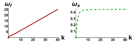
Figure 1: Plot of $\omega_{f}$ vs $k$ (left panel) and $\omega_{s}$ vs $k$ (right panel) when $\alpha=0.4$, $\mu=10^{-6}$, $\nu=5\times 10^{5}$, $\gamma_{2}=0.4$, and $\gamma_{3}=0.6$.

where $A=k^{2}+H_{1}$, $B=1+\gamma_{1}-\gamma_{1}\gamma_{3}+\gamma_{2}k^{2}+\gamma_{2}H_{1}$, and $C=\gamma_{1}\gamma_{2}-\gamma_{1}\gamma_{2}\gamma_{3}$. In Eq. (20), to get real and positive value of $\omega$, the condition $B^{2}>4AC$ should be satisfied. The positive and negative signs in Eq. (20) correspond to the fast ($\omega_{f}$) and slow ($\omega_{s}$) DIA modes. The fast DIA mode corresponds to the case in which both inertial dust and ion components oscillate in phase with the inertialess electrons. On the other hand, the slow DIA mode corresponds to the case in which only one of the inertial components oscillates in phase with inertialess electrons, but the other inertial component oscillates in anti-phase with them [29, 30]. We have numerically analyzed the fast and slow DIA modes in Fig. 1 in the presence of non-thermal electrons. Figure 1 (left panel) indicates that the frequency of the DIAWs can be higher than ion-plasma frequency. In this regard, we note that in absence of dust, the frequency of the ion-acoustic waves is always less than the ion-plasma or ion-Langmuir frequency. However, the phase speed of the DIAWs increases with the magnitude of the dust charge ($Z_{d}$) and dust number density ($n_{d0}$). This is due to the extra space charge electric field created by the highly negatively charged dust grains. This is theoretically predicted by Shukla and Silin [31] and experimentally observed by Barkan et al. [32]. Thus, as the magnitude of the dust charge ($Z_{d}$) or dust number density ($n_{d0}$) increases, the frequency of the DIAWs increases, even it can exceed the ion-plasma or ion-Langmuir frequency. On the other hand, the dispersion curve of slow DIA mode shown in Fig. 1 (right panel) clearly indicates that the frequency of the slow DIA mode is always less than the ion-plasma or ion-Langmuir frequency even in the presence of highly negatively charged dust.

For second order harmonics, equations can be found from the next order of $\epsilon$ (with $m=2$ and $l=1$) as

$$n_{d1}^{(2)}=-\frac{\gamma_{1}k^{2}}{\omega^{2}}\phi_{1}^{(2)}-\bigg{[}\frac{2(\gamma_{1}k\omega-\gamma_{1}v_{g}k^{2})}{i\omega^{3}}\bigg{]}\frac{\partial\phi_{1}^{(1)}}{\partial\xi},$$ (21)

$$u_{d1}^{(2)}=-\frac{\gamma_{1}k}{\omega}\phi_{1}^{(2)}-\bigg{[}\frac{\gamma_{1}\omega-\gamma_{1}v_{g}k}{i\omega^{2}}\bigg{]}\frac{\partial\phi_{1}^{(1)}}{\partial\xi},$$ (22)

$$n_{i1}^{(2)}=\frac{k^{2}}{\omega^{2}-\gamma_{2}k^{2}}\phi_{1}^{(2)}+\bigg{[}\frac{2k\omega(\omega-v_{g}k)}{i(\omega^{2}-\gamma_{2}k^{2})^{2}}\bigg{]}\frac{\partial\phi_{1}^{(1)}}{\partial\xi},$$ (23)

$$u_{i1}^{(2)}=\frac{k\omega}{\omega^{2}-\gamma_{2}k^{2}}\phi_{1}^{(2)}+\bigg{[}\frac{(\omega-v_{g}k)}{i(\omega^{2}-\gamma_{2}k^{2})^{2}}\bigg{]}\frac{\partial\phi_{1}^{(1)}}{\partial\xi}$$

$$+\bigg{[}\frac{(\omega^{2}+\gamma_{2}k^{2})}{i(\omega^{2}-\gamma_{2}k^{2})^{2}}\bigg{]}\frac{\partial\phi_{1}^{(1)}}{\partial\xi},\$$ (24)

with the compatibility condition, we have obtained the group speed of IAWs as

$$v_{g}=\frac{\gamma_{1}\gamma_{3}\omega^{5}+2\gamma_{1}\gamma_{2}k^{2}\omega^{3}-2\gamma_{1}\gamma_{2}\gamma_{3}k^{2}\omega^{3}-\gamma_{1}\omega^{5}+\mathcal{F}_{1}}{\gamma_{1}\gamma_{2}^{2}\gamma_{3}k^{5}-2\gamma_{1}\gamma_{2}\gamma_{3}k^{3}\omega^{2}+\mathcal{F}_{2}},$$ (25)

where

$$\mathcal{F}_{1}=\gamma_{1}\gamma_{2}^{2}\gamma_{3}k^{4}\omega-\omega^{5}+\omega^{7}-2\gamma_{2}\omega^{5}k^{2}+\gamma_{2}^{2}\omega^{3}k^{4}-\gamma_{1}\gamma_{2}^{2}k^{4}\omega,$$

$$\mathcal{F}_{2}=\gamma_{1}\gamma_{3}k\omega^{4}-\gamma_{1}k\omega^{4}+2\gamma_{1}\gamma_{2}k^{3}\omega^{2}-k\omega^{4}-\gamma_{1}\gamma_{2}^{2}k^{5}.\$$

The coefficients of the $\epsilon$ when $m=2$ with $l=2$ provides the second order harmonic amplitudes which are found to be proportional to $|\phi_{1}^{(1)}|^{2}$

$$n_{d2}^{(2)}=H_{4}|\phi_{1}^{(1)}|^{2},$$ (26)

$$u_{d2}^{(2)}=H_{5}|\phi_{1}^{(1)}|^{2},$$ (27)

$$n_{i2}^{(2)}=H_{6}|\phi_{1}^{(1)}|^{2},$$ (28)

$$u_{i2}^{(2)}=H_{7}|\phi_{1}^{(1)}|^{2},$$ (29)

$$\phi_{2}^{(2)}=H_{8}|\phi_{1}^{(1)}|^{2},\$$ (30)

where

$$H_{4}=\frac{3\gamma_{1}^{2}k^{4}-2\gamma_{1}k^{2}\omega^{2}H_{8}}{2\omega^{4}},$$

$$H_{5}=\frac{\gamma_{1}^{2}k^{3}-2\gamma_{1}k\omega^{2}H_{8}}{2\omega^{3}},$$

$$H_{6}=\frac{2k^{2}H_{8}(\omega^{2}-\gamma_{2}k^{2})^{2}+k^{4}(\gamma_{2}k^{2}+3\omega^{2})}{2(\omega^{2}-\gamma_{2}k^{2})^{3}},$$

$$H_{7}=\frac{2k(H_{8}+\gamma_{2}H_{6})(\omega^{2}-\gamma_{2}k^{2})^{2}+k^{3}\omega^{2}+\gamma_{2}k^{5}}{2\omega(\omega^{2}-\gamma_{2}k^{2})^{2}},$$

$$H_{8}=\{k^{4}\omega^{4}(3\omega^{2}+\gamma_{2}k^{2})-3\gamma_{1}^{2}k^{4}(1-\gamma_{3})(\omega^{2}-\gamma_{2}k^{2})^{3}$$

$$-2\omega^{4}H_{2}(\omega^{2}-\gamma_{2}k^{2})^{3}\}/6k^{2}\omega^{4}(\omega^{2}-\gamma_{2}k^{2})^{3}.\$$

Again, when ($m=3$ with $l=0$) and ($m=2$ with $l=0$), we find these relations

$$n_{d0}^{(2)}=H_{9}|\phi_{1}^{(1)}|^{2},$$ (31)

$$u_{d0}^{(2)}=H_{10}|\phi_{1}^{(1)}|^{2},$$ (32)

$$n_{i0}^{(2)}=H_{11}|\phi_{1}^{(1)}|^{2},$$ (33)

$$u_{i0}^{(2)}=H_{12}|\phi_{1}^{(1)}|^{2},$$ (34)

$$\phi_{0}^{(2)}=H_{13}|\phi_{1}^{(1)}|^{2},\$$ (35)

where

$$H_{9}=\frac{2\gamma_{1}^{2}v_{g}k^{3}+\gamma_{1}^{2}k^{2}\omega-\gamma_{1}\omega^{3}H_{13}}{v_{g}^{2}\omega^{3}},$$

$$H_{10}=\frac{\gamma_{1}^{2}k^{2}-\gamma_{1}\omega^{2}H_{13}}{v_{g}\omega^{2}},$$

$$H_{11}=\frac{H_{13}(\omega^{2}-\gamma_{2}k^{2})^{2}+2v_{g}k^{3}\omega+\gamma_{2}k^{4}+k^{2}\omega^{2}}{(\gamma_{2}-v_{g}^{2})(\omega^{2}-\gamma_{2}k^{2})^{2}},$$

$$H_{12}=\frac{(H_{1}3+\gamma_{2}H_{11})(\omega^{2}-\gamma_{2}k^{2})^{2}+k^{2}\omega^{2}+\gamma_{2}k^{4}}{v_{g}(\omega^{2}-\gamma_{2}k^{2})^{2}},$$

$$H_{13}=\frac{v_{g}^{2}k^{2}\omega^{3}(\gamma_{2}k^{2}+\omega^{2}+2v_{g}k\omega)-\mathcal{F}_{3}}{\omega^{3}(\omega^{2}-\gamma_{2}k^{2})^{2}\times\mathcal{F}_{4}},\$$

where

$$\mathcal{F}_{3}=(1-\gamma_{3})(v_{g}^{2}-\gamma_{2})(\omega^{2}-\gamma_{2}k^{2})^{2}(\gamma_{1}^{2}k^{2}\omega+2\gamma_{1}^{2}v_{g}k^{3})$$

$$+2v_{g}^{2}\omega^{3}H_{2}(v_{g}^{2}-\gamma_{2})(\omega^{2}-\gamma_{2}k^{2})^{2},$$

$$\mathcal{F}_{4}=v_{g}^{2}H_{1}(v_{g}^{2}-\gamma_{2})-v_{g}^{2}-\gamma_{1}(1-\gamma_{3})(v_{g}^{2}-\gamma_{2}).\$$

Now, we develop the standard NLSE by substituting all the above equations into third order harmonic modes ($m=3$ with $l=1$):

$$i\frac{\partial\Phi}{\partial\tau}+P\frac{\partial^{2}\Phi}{\partial\xi^{2}}+Q|\Phi|^{2}\Phi=0,$$ (36)

where $\Phi=\phi_{1}^{(1)}$ for simplicity. In Eq. (36), $P$ can be written as

$$P=\frac{\mathcal{F}_{5}-\omega^{4}(\omega^{2}-\gamma_{2}k^{2})^{3}}{\omega(\omega^{2}-\gamma_{2}k^{2})\times\mathcal{F}_{6}},\$$

where

$$\mathcal{F}_{5}=\omega^{4}(\omega-v_{g}k)\{2k\omega(\gamma_{2}k-v_{g}\omega)+(\omega-v_{g}k)(\omega^{2}+\gamma_{2}k^{2})\}$$

$$+\gamma_{1}(1-\gamma_{3})(\omega-v_{g}k)(\omega-3v_{g}k)(\omega^{2}-\gamma_{2}k^{2})^{3},$$

$$\mathcal{F}_{6}=2k^{2}\omega^{4}+2\gamma_{1}k^{2}(1-\gamma_{3})(\omega^{2}-\gamma_{2}k^{2})^{2},\$$

and also $Q$ can be written as

$$Q=\frac{\mathcal{F}_{7}-\omega^{3}(\omega^{2}k^{2}+\gamma_{2}k^{4})(H_{6}+H_{11})-2k^{3}\omega^{4}(H_{7}+H_{12})}{\mathcal{F}_{6}},\$$

where

$$\mathcal{F}_{7}=\big{[}\omega^{3}\{3H_{3}+2H_{2}(H_{8}+H_{13})\}-\gamma_{1}k^{2}\omega(1-\gamma_{3})(H_{4}+H_{9})$$

$$-2\gamma_{1}k^{3}(1-\gamma_{3})(H_{5}+H_{10})\big{]}(\omega^{2}-\gamma_{2}k^{2})^{2}.\$$

The space and time evolution of the DIAWs in the plasma medium are directly governed by the dispersion ($P$) and nonlinear ($Q$) coefficients of NLSE and are indirectly governed by different plasma parameters such as $\alpha$, $\mu$, $\nu$, $\gamma_{2}$, and $\gamma_{3}$. Thus, these plasma parameters significantly affect the stability conditions of DIAWs.

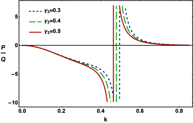
Figure 2: Plot of $P/Q$ vs $k$ for various values of $\gamma_{2}$ when $\alpha=0.4$, $\mu=10^{-6}$, $\nu=5\times 10^{5}$, and $\gamma_{3}=0.6$.

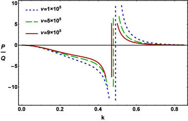
Figure 3: Plot of $P/Q$ vs $k$ for various values of $\nu$ when $\alpha=0.4$, $\mu=10^{-6}$, $\gamma_{2}=0.4$, and $\gamma_{3}=0.6$.

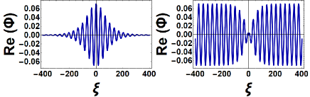
Figure 4: Bright (left panel) and dark (right panel) envelope solitons when other plasma parameters are $\tau=0$, $\psi_{0}=0.005$, $U=0.4$, $\Omega_{0}=0.4$, $\alpha=0.4$, $\mu=10^{-6}$, $\nu=5\times 10^{5}$, $\gamma_{2}=0.4$, and $\gamma_{3}=0.6$.

4 Modulational instability and Envelope Solitons

The stable and unstable parametric regimes of DIAWs are organised by the sign of $P$ and $Q$ of Eq. (36). When $P$ and $Q$ has the same sign (i.e., $P/Q>0$), the evolution of DIAWs amplitude is modulationally unstable in the presence of external perturbations. On the other hand, when $P$ and $Q$ has opposite sign (i.e., $P/Q<0$), the DIAWs are modulationally stable in the presence of external perturbations. So, the plot of $P/Q$ against $k$ yields stable and unstable parametric regimes of the DIAWs. The point at which the transition of $P/Q$ curve intersects with the $k$-axis is known as the critical wave number $k~{}(=k_{c})$.

The bright (when $P/Q>0$) and dark (when $P/Q<0$) envelope solitonic solutions can be written, respectively, as

$$\Phi(\xi,\tau)=\left[\psi_{0}~{}\mbox{sech}^{2}\left(\frac{\xi-U\tau}{W}\right)\right]^{\frac{1}{2}}$$

$$\times\exp\left[\frac{i}{2P}\left\{U\xi+\left(\Omega_{0}-\frac{U^{2}}{2}\right)\tau\right\}\right],$$ (37)

$$\Phi(\xi,\tau)=\left[\psi_{0}~{}\mbox{tanh}^{2}\left(\frac{\xi-U\tau}{W}\right)\right]^{\frac{1}{2}}$$

$$\times\exp\left[\frac{i}{2P}\left\{U\xi-\left(\frac{U^{2}}{2}-2PQ\psi_{0}\right)\tau\right\}\right],$$ (38)

where $\psi_{0}$ is the amplitude of localized pulse for both bright and dark envelope solitons, $U$ is the propagation speed of the localized pulse, $W$ is the soliton width, and $\Omega_{0}$ is the oscillating frequency at $U=0$. The soliton width $W$ and the maximum amplitude $\psi_{0}$ are related as $W=\sqrt{2\mid P/Q\mid/\psi_{0}}$. We have depicted the bright (left panel) and dark (right panel) envelope solitons in Fig. 4.

5 Results and discussions

Now, we would like to numerically analyze the stability conditions of the DIAWs in the presence of non-thermal electrons. The mass and charge state of the plasma species, even their number density, are important factors in recognizing the stability conditions of the DIAWs in DPM [1, 30, 33, 34, 35, 36]. The mass of the dust grains is comparable to the mass of the protons. In a general picture of the DPM, dust grains are massive (million to billion times heavier than the protons) and their sizes range from nanometres to millimetres. Dust grains may be metallic, conducting, or made of ice particulates. The size and shape of dust grains will be different, unless they are man-made. The dust grains are million to billion times heavier than the protons, and typically, a dust grain acquires one thousand to several hundred thousand elementary charges [1, 30, 33, 34, 35, 36].

It may be noted here that in DAWs, the mass of the dust grains provides the moment of inertia, and the thermal pressure of the electrons and ions provides the restoring force in a three component DPM. On the other hand, in DIAWs, the mass of the ion provides the moment of inertia, and the thermal pressure of the electron provides the restoring force in the presence of immobile dust grains. In this article, we consider three component dusty plasma model having inertial warm positive ions and negative dust grains, and interialess non-thermal electrons. It may be noted here that in the DIAWs, if anyone considers the thermal effects of the ions then it is important to consider the moment of inertia of the ions along with the dust grains in the presence of inertialess electrons. This means that the consideration of the pressure term of the ions highly contributes to the moment of inertia along with inertial dust grains to generate DIAWs in a DPM having inertialess electrons. In our present analysis, we have considered that $m_{d}=10^{6}m_{i}$, $Z_{d}=(10^{3}\thicksim 10^{5})Z_{i}$, and $T_{e}=10T_{i}$.

The effects of ion and electron temperature on MI conditions of DIAWs can be observed from Fig. 2 and it is clear from this figure that (a) it is really interesting that both modulaltionally stable and unstable parametric regimes are allowed; (b) the DIAWs are modulationally stable for small values of $k$ while modulationally unstable for large values of $k$; (c) the critical wave number $k_{c}$ decreases (increases) with increasing ion (electron) temperature for a constant value of $Z_{i}$ (via $\gamma_{2}$). So, ion and electron temperature play an opposite role in recognizing the modulationally stable and unstable parametric regimes of DIAWs. Figures 3 can reflect the effects of the charge state of inertial warm ions and negatively charged dust grains on the instability criterion of DIAWs in the presence of non-thermal electrons (via $\nu$). The DIAWs become unstable for small (large) values of $k$ as we increase the charge state of the inertial negatively charged dust grains (warm ions). Finally, from Fig. 4, it can be seen that the bright (dark) envelope solitons associated with the unstable (stable) parametric regimes of DIAWs are allowed by the plasma model.

6 Conclusion

In this work, we have considered the moment of inertia of the warm ions along with negatively charged dust grains and inertialess non-thermal electrons for studying the conditions of MI of the DIAWs. By employing RPM, we have derived the NLSE (36) from a set of basic equations, and have studied the formation of the electrostatic envelope solitons associated with DIAWs in an unmagnnetized DPM. The consideration of the moment of inertia of the warm ions along with the negatively charged dust grains in a three component DPM has significantly changed the dynamics of DPM as well as the instability conditions of the DIAWs. We, finally, hope that the findings of our present investigation should be useful in understanding the mechanism of the formation of electrostatic envelope solitons in a three component DPM (viz., cometary tails [3], the magnetosphere of the Jupiter and the Saturn [4], interstellar medium [5, 6], in the galactic centre [6], and the Earth’s ionosphere [9], etc.).

References

[1] P.K. Shukla and A.A. Mamun, Introduction to Dusty Plasma Physics, Institute of Physics, Bristol, 2002.
[2] M. Shahmansouri and A.A. Mamun, J. Plasma Physics 80, 593 (2014).
[3] H. Alinejad, Astrophys. Space Sci. 327, 131 (2010).
[4] A. Paul and A. Bandyopadhyay, Astrophys. Space Sci. 361, 172 (2016).
[5] G. Banerjee and S. Maitra, Phys. Plasmas 23, 123701 (2016).
[6] S. Sardar, et al., Phys. Plasmas 24, 063705 (2017).
[7] M.R. Amin, et al., Phys. Rev. E 58, 6517 (1998).
[8] S.K. El-Labany, et al., Phys. Plasmas 22, 073702 (2015).
[9] N.S. Saini and I. Kourakis, Phys. Plasmas 15, 123701 (2008).
[10] A.P. Misra and A. Roy Chowdhury, Eur. Phys. J. D 39, 49 (2006).
[11] G.S. Selwyn, et al., J. Vac. Sci. Technol. A 11, 1132 (1993).
[12] H. Kersten, et al., Contrib. Plasma Phys. 411, 598 (2001).
[13] A.J. Hundhausen, et al., J. Geophys. Res. 72, 1979 (1967).
[14] R.A. Cairns, et al., Geophys. Res. Lett. 22, 2709 (1995).
[15] N.A. Chowdhury, et al., Chaos 27, 093105 (2017).
[16] N.A. Chowdhury, et al., Phys. plasmas 24, 113701 (2017).
[17] M.H. Rahman, et al., Chinese J. Phys. 56, 2061 (2018).
[18] M.H. Rahman, et al., Phys. Plasmas 25, 102118 (2018).
[19] N.A. Chowdhury, et al., Vacuum 147, 31 (2018).