The resurgent structure of quantum knot invariants

Abstract.

The asymptotic expansion of quantum knot invariants in complex Chern-Simons theory gives rise to factorially divergent formal power series. We conjecture that these series are resurgent functions whose Stokes automorphism is given by a pair of matrices of $q$-series with integer coefficients, which are determined explicitly by the fundamental solutions of a pair of linear $q$-difference equations. We further conjecture that for a hyperbolic knot, a distinguished entry of those matrices equals to the Dimofte-Gaiotto-Gukov 3D-index, and thus is given by a counting of BPS states. We illustrate our conjectures explicitly by matching theoretically and numerically computed integers for the cases of the $4_{1}$ and the $5_{2}$ knots.

1. Introduction

1.1. Asymptotic expansions in perturbative quantum field theory

Perturbative expansions in quantum field theories are often mathematically defined but typically lead to factorially divergent formal power series. Important examples are the perturbative expansions of the partition function of 3-dimensional manifolds (with, or without boundary) in complex Chern-Simons theory with arbitrary gauge group. For instance, in [GLMn08] it was shown that the LMO invariant of a 3-manifold (which is the perturbative expansion of the Witten-Reshetikhin-Turaev invariant at the trivial flat collection and arbitrary gauge group), is a Gevrey-1 formal power series, that is a formal power series whose $n$th coefficient is bounded by $n!C^{n}$ for some positive constant $C$. Said differently, these perturbative expansions have Borel transforms which are germs of holomorphic functions at the origin.

In [Gar08] it was conjectured that the perturbative expansions in complex Chern-Simons theory are resurgent functions, and more precisely that they have analytic continuation as multivalued functions in the complex plane minus a discrete and computable set of points, placed in finitely many vertical lines in the complex plane. These vertical lines are formed by an infinite towers of singularities, with a $2\pi{\rm i}$ periodicity. The position of these singularities is dictated by the values of the complex Chern-Simons function (a $\mathbbm{C}/2\pi{\rm i}\mathbbm{Z}$-valued function) on the set of flat connections.

1.2. Resurgence in complex Chern-Simons theory

In what follows, we will identify the partition function of complex Chern-Simons theory with the state integral of Andersen-Kashaev in [AK14], following the ideas of Hikami, Dimofte et al [Hik07, DGLZ09]. Although this identification has not been derived from first principles, it turns out to have a number of startling consequences. We will focus on manifolds of the form $M=\mathbb{S}^{3}\backslash\mathcal{K}$, where $\mathcal{K}$ is a hyperbolic knot.

Our goal is to give an explicit description of the resurgent structure of the formal power series of perturbative Chern-Simons theory in terms of a fundamental solution of a pair of linear $q$-difference equation and a matrix of integers. We will describe the general story first, and illustrate it with concrete examples later.

We will denote by $\mathcal{P}$ the set of critical points of the complex Chern-Simons action and by $\sigma$ a typical critical point. Given our identification of Chern-Simons theory with state integrals, it turns out that the set $\mathcal{P}$ coincides with the set of critical points of the integrand of the state integral, an effectively computable set of algebraic numbers. The critical values of the complex Chern-Simons function are labeled by $\sigma$ and an integer $\mu$ (often called “multicovering”):

$$\text{CS}(\sigma;\mu)={V(\sigma)\over 2\pi}-2\pi{{\rm i}}\mu,\qquad\mu\in\mathbbm{Z}.$$ (1)

We conjecture that the corresponding transseries $\Phi_{\sigma,\mu}$ satisfy the translation invariance property

$$\Phi_{\sigma,\mu}(\tau)=\tilde{q}^{\mu}\,\Phi_{\sigma}(\tau),\qquad\tilde{q}={\rm e}^{-2\pi{\rm i}/\tau},$$ (2)

where $\Phi_{\sigma}(\tau)$ is the conventional asymptotic expansion of the state integral around the saddle point $\sigma$. It has the form

$$\Phi_{\sigma}(\tau)=\exp\left({V(\sigma)\over 2\pi\tau}\right)\varphi_{\sigma}(\tau),\qquad\varphi_{\sigma}(\tau)\in\mathbbm{C}[[\tau]].$$ (3)

As a consequence, all the Stokes automorphisms acting on $\Phi_{\sigma,\mu}$ are packaged in two Stokes automorphism matrices $\mathsf{S}^{+}(q)$, $\mathsf{S}^{-}(q^{-1})$, which are matrices of $q$- and $q^{-1}$-series respectively, and each of which encodes Stokes automorphism across a half-plane. Their detailed definition is given in Section 5.1.

An important feature of state integrals is that they depend on additional parameters and this leads to a system of a pair of linear $q$-difference equations, one in the upper half-plane and another in the lower half-plane [GK17]. In our examples, these linear $q$-difference equations have explicit sets of fundamental solutions. We conjecture that

Conjecture 1.

(a) $\mathsf{S}^{\pm}(q)$ are bilinear functions of two fundamental solutions of the pair of linear $q$-difference equations.
(b) $\mathsf{S}^{\pm}(q)$ satisfy the inversion relation

$$\mathsf{S}^{+}(q)^{T}\mathsf{S}^{-}(q)=\mathbf{1}\,.$$ (4)

(c) $\mathsf{S}^{\pm}(q)$ are uniquely determined by $\mathsf{S}^{+}(0)$, $\mathsf{S}^{-}(0)$ and a pair of fundamental solutions to the pair of linear $q$-difference equations.

The above matrices $\mathsf{S}^{\pm}$ uniquely determine the collection of transseries $\Phi_{\sigma,\mu}(\tau)$ for all $(\sigma,\mu)$ via an abstract Riemann-Hilbert correspondence first pointed out in [Vor83] and developed recently in [GMN10, IMnS19, KS20]. Note that this transcendental correspondence converts the difficult problem of computing coefficients of $\Phi_{\sigma,\mu}(\tau)$ (typically, one can not compute more than a couple of hundred coefficients) into the much easier problem of computing fundamental solutions of linear $q$-difference equations, up to a matrix of unknown integers.

Given a hyperbolic knot $\mathcal{K}$ there is a distinguished critical point $\sigma_{1}$ (the geometric representation, corresponding to the complete hyperbolic structure), and in that case we conjecture a precise relation between the entry $\mathsf{S}^{+}_{\sigma_{1},\sigma_{1}}(q)$ of the matrix $\mathsf{S}^{+}(q)$ and the (rotated) 3D-index of Dimofte-Gaiotto-Gukov [DGG14, DGG13].

Conjecture 2.

We have:

$$\mathsf{S}^{+}_{\sigma_{1}\sigma_{1}}(q)=\,\mathrm{Ind}_{\mathcal{K}}^{\mathrm{rot}}(q)\,.$$ (5)

We recall that the 3D-index $\mathcal{I}_{\mathcal{K}}(m,e)(q)$ associated to a knot $\mathcal{K}$ is labeled by two integers $(m,e)$. It counts BPS states in a three-dimensional, $\mathcal{N}=2$ supersymmetric theory $T_{M}$ which can be associated to the manifold $M=\mathbb{S}^{3}\backslash\mathcal{K}$ [DGG14]. The rotated index is then given by

$$\mathrm{Ind}_{\mathcal{K}}^{\mathrm{rot}}(q)=\sum_{e\in\mathbb{Z}}\mathcal{I}_{\mathcal{K}}(0,e)(q).$$ (6)

The relation in (5) between the resurgent structure of complex Chern–Simons theory and a counting of BPS states in the corresponding supersymmetric theory was anticipated in [Mn19, GGMn20b].

We emphasize that although the state integrals and their perturbation theory are well-defined, the above picture is largely conjectural. However, it fits well with the work of Kontsevich-Soibelman [KS11], as well as with a lecture of Kontsevich on June 30, 2020 [Kon20], and it paves the way for a deeper understanding of the topological/physical meaning of the integers appearing in $\mathsf{S}^{\pm}$.

We should point out that the above theory in fact has little to do with knots and 3-manifolds and complex Chern-Simons theory, and little to do with the Bloch group, but appears to be part of a larger combinatorial structure. This is apparent in the data needed to define the formal power series of [DG13, DG18] as well as the data needed to define $q$-hypergeometric Nahm sums (and thus their asymptotic expansion at roots of unity [GZa]) and the data needed to define state integrals [GK17]. This combinatorial structure is sometimes called a $K_{2}$-Lagrangian, or an extended symplectic group.

We will illustrate the above conjectures concretely for the invariants of the two simplest hyperbolic knots, the $4_{1}$ and the $5_{2}$ knots. Some aspects of the resurgent structure of complex Chern–Simons theory for the $4_{1}$ knot were studied in [GMnP, GH18], but they focused on the “classical” transseries $\Phi_{\sigma}(\tau)$ (i.e. they didn’t address the resurgent structure of the tower of singularities). The resurgent problem in the case of compact $\mathrm{SU}(2)$ Chern–Simons theory was addressed in [CG11, GMnP], where complete towers of Stokes constants were explicitly computed for some Seifert three-manifolds.

This paper is, in a sense, a sequel to [GZc] and [GZb] which the reader can consult for further information, motivation, historical presentation, as well as for the connection with the asymptotics of the Kashaev invariant and with the quantum modularity conjecture.

Note that our notation $\varphi_{\sigma}(\tau)$ from Equation (3) corresponds to the notation $\Phi^{(\sigma)}_{0}(2\pi{\rm i}x)$ of [GZc]. In particular, the coefficient of $\tau^{n}$ in $\varphi_{\sigma}(\tau)$ is (up to multiplication by an eighth root of unity and the square root of an nonzero element of $F_{\sigma}$) in $(2\pi{\rm i})^{n}F_{\sigma}$, where $F_{\sigma}$ is the trace field of $\sigma$.

2. The equation $(1-x)(1-x^{-1})=1$ and the $4_{1}$ knot

The state integral of the $4_{1}$ knot is given by Equation (39) below with $(A,B)=(1,2)$ and $\mu=\lambda=0$. The critical points of the integrand are solutions of the algebraic equation

$$(1-x)(1-x^{-1})=1.$$ (7)

The latter has two solutions $\xi_{1}={\rm e}^{2\pi{\rm i}/6}$ and $\xi_{2}={\rm e}^{-2\pi{\rm i}/6}$ which lie in the number field $\mathbbm{Q}(\sqrt{-3})$, the trace field of the $4_{1}$ knot. The corresponding series $\Phi_{\sigma_{j}}(\tau)$ satisfy the relation $\Phi_{\sigma_{2}}(\tau)={\rm i}\Phi_{\sigma_{1}}(-\tau)$ and the first few terms of $\varphi_{\sigma_{1}}(\tau/(2\pi{\rm i}))\in 3^{-1/4}\mathbbm{Q}(\sqrt{-3})[[\tau]]$ are given by

$$\varphi_{\sigma_{1}}\left(\frac{\tau}{2\pi{\rm i}}\right)=\frac{1}{\sqrt[4]{3}}\,\Bigl{(}1\,+\,\frac{11\tau}{72\sqrt{-3}}\,+\,\frac{697\tau^{2}}{2\,(72\sqrt{-3})^{2}}\,+\,\frac{724351\tau^{3}}{30\,(72\sqrt{-3})^{3}}\,+\,\cdots\Bigr{)}\,.$$ (8)

The exponent in (3) involves the hyperbolic volume of the $4_{1}$ knot complement

$$V(\sigma_{1})=V=2{\rm Im}\,{\rm Li}_{2}({\rm e}^{{\rm i}\pi/3})=2.029883\dots\,.$$ (9)

The two series $\Phi_{\sigma_{j}}(\tau)$ for $j=1,2$ form a vector

$$\Phi(\tau)=\begin{pmatrix}\Phi_{\sigma_{1}}(\tau)\\ \Phi_{\sigma_{2}}(\tau)\end{pmatrix}$$ (10)

that also appears in the refined quantum modularity conjecture [GZc]. $\Phi(\tau)$ is the vector of series whose description in Borel plane we wish to give.

Consider the linear $q$-difference equation

$$y_{m+1}(q)-(2-q^{m})y_{m}(q)+y_{m-1}(q)=0\qquad(m\in\mathbbm{Z})\,.$$ (11)

It has a fundamental solution set given by the columns of the following matrix

$$W_{m}(q)=\begin{pmatrix}G^{0}_{m}(q)&G^{1}_{m}(q)\\ G^{0}_{m+1}(q)&G^{1}_{m+1}(q)\end{pmatrix},$$ (12)

where $G^{0}_{m}(q)$ and $G^{1}_{m}(q)$ are defined by

$$G^{0}_{m}(q) =\sum_{n=0}^{\infty}(-1)^{n}\frac{q^{n(n+1)/2+mn}}{(q;q)_{n}^{2}}$$ (13a)

$$G^{1}_{m}(q) =\sum_{n=0}^{\infty}(-1)^{n}\frac{q^{n(n+1)/2+mn}}{(q;q)_{n}^{2}}\left(2m+E_{1}(q)+2\sum_{j=1}^{n}\frac{1+q^{j}}{1-q^{j}}\right)\,,$$ (13b)

and $E_{1}(q)=1-4\sum_{n=1}^{\infty}q^{n}/(1-q^{n})$ is the Eisenstein series.

It is easy to see that $G^{0}_{m}$ satisfies (11). Indeed, $G^{0}_{m}(q)=\sum_{n=0}^{\infty}a_{n,-m}(q)^{-1}$ where $a_{n,m}(q)$ is given in (34) below. Equations (35a)-(35c), applied to $a_{n,-m}(q)^{-1}$ conclude the result. A similar proof applies for $G^{1}_{m}$. Another way to do so is to use the state integral (39) (with $(A,B)=(1,2)$) and show that the latter satisfies the linear $q$-difference equation (11) in two ways, one with respect to the variable $\lambda$ and another with respect to the variable $\mu$.

The fundamental solution $W_{m}(q)$ satisfies

$$\det(W_{m}(q))=2$$ (14)

and the symmetry

$$W_{m}(q^{-1})=W_{-m}(q)\begin{pmatrix}1&0\\ 0&-1\end{pmatrix}\,,$$ (15)

and the orthogonality

$$\frac{1}{2}W_{m}(q)\begin{pmatrix}0&1\\ -1&0\end{pmatrix}W_{m}(q)^{T}=\begin{pmatrix}0&1\\ -1&0\end{pmatrix}\,.$$ (16)

for all integers $m$, as well as

$$\frac{1}{2}W_{m}(q)\begin{pmatrix}0&1\\ -1&0\end{pmatrix}W_{\ell}(q)^{T}\in\mathrm{SL}(2,\mathbbm{Z}[q,1/q])$$ (17)

for all integers $m,\ell$. The $\mathsf{S}$ matrix is given by

$$\mathsf{S}^{+}(q) ={1\over 2}\begin{pmatrix}0&1\\ 1&1\end{pmatrix}W_{-1}(q)\begin{pmatrix}0&1\\ 1&0\end{pmatrix}W_{-1}(q)^{T}\begin{pmatrix}0&-1\\ 1&2\end{pmatrix},$$ (18a)

$$\mathsf{S}^{-}(q) ={1\over 2}\begin{pmatrix}-1&-1\\ 0&1\end{pmatrix}W_{-1}(q)\begin{pmatrix}0&1\\ 1&0\end{pmatrix}W_{-1}(q)^{T}\begin{pmatrix}1&0\\ -2&1\end{pmatrix}\,.$$ (18b)

The above matrix $\mathsf{S}$ satisfies Equation (4).

3. The equation $x^{-2}(1-x)^{3}=1$ and the $5_{2}$ knot

The state integral of the $5_{2}$ knot is given by Equation (39) below with $(A,B)=(2,3)$ and $\mu=\lambda=0$. The critical points of the integrand are solutions of the algebraic equation

$$x^{-2}(1-x)^{3}=1\,.$$ (19)

The above equation (which defines a cubic field of discriminant $-23$, the trace field of the $5_{2}$ knot) has three solutions $\xi_{1}=0.78492+1.30714\dots\rm i$, $\xi_{2}=0.78492-1.30714\dots\rm i$ and $\xi_{3}=0.43016\dots$, corresponding to the geometric representation, its conjugate and the real representation. The corresponding series $\Phi_{\sigma_{j}}(\tau)$ satisfy $\Phi_{\sigma_{2}}(\tau)=-{\rm i}\overline{\Phi}_{\sigma_{1}}(-\tau)$ and the first few terms of $\phi_{\sigma_{j}}(\tau/(2\pi{\rm i}))$ are given by

$$\varphi_{\sigma_{j}}\left(\frac{\tau}{2\pi{\rm i}}\right) =\left(\frac{-3\xi_{j}^{2}+3\xi_{j}-2}{23}\right)^{1/4}\left(1+\frac{33\xi_{j}^{2}+242\xi_{j}-245}{2^{2}\cdot 23^{2}}\tau+\frac{100250\xi_{j}^{2}-12643\xi_{j}+2732}{2^{5}\cdot 23^{3}}\tau^{2}\right.$$

$$+\frac{-50198891\xi_{j}^{2}+35443870\xi_{j}-79016748}{2^{7}\cdot 3\cdot 5\cdot 23^{5}}\tau^{3}$$

$$\left.+\frac{-3809943572\xi_{j}^{2}+1861268771\xi_{j}+1015686665}{2^{11}\cdot 3\cdot 5\cdot 23^{6}}\tau^{4}+\dots\right)\,.$$ (20)

The exponent in (3) involves

$$V(\sigma_{1})=2.821\ldots+1.379\ldots{\rm i},\;V(\sigma_{2})=-2.821\ldots+1.379\ldots{\rm i},\;V(\sigma_{3})=-2.758\ldots$$ (21)

where $\Re\,V(\sigma_{1})$ is the hyperbolic volume of the $5_{2}$ knot complement, and $\Im\,V(\sigma_{1})=\Im\,V(\sigma_{2})$ the Chern-Simons action. The three series $\Phi_{\sigma_{j}}(\tau)$ for $j=1,2,3$ form a vector

$$\Phi(\tau)=\left(\begin{array}[]{c}\Phi_{\sigma_{1}}(\tau)\\ \Phi_{\sigma_{2}}(\tau)\\ \Phi_{\sigma_{3}}(\tau)\end{array}\right).$$ (22)

Consider the linear $q$-difference equation

$$y_{m}(q)-3y_{m+1}(q)+(3-q^{2+m})y_{m+2}(q)-y_{m+3}(q)=0.$$ (23)

The above equation has a fundamental solution set given by the columns of the following matrix

$$W_{m}(q)=\begin{cases}W_{m}^{+}(q),\quad&|q|<1,\\ \begin{pmatrix}0&0&1\\ 0&1&0\\ 1&0&0\end{pmatrix}W_{-m-2}^{-}(q^{-1})\begin{pmatrix}1&0&0\\ 0&-1&0\\ 0&0&1\end{pmatrix},\quad&|q|>1.\end{cases}$$ (24)

where the matrices $W_{m}^{\varepsilon}(q)$ with $\varepsilon=\pm$ are respectively

$$W^{\varepsilon}_{m}(q)=\begin{pmatrix}H^{\varepsilon}_{0,m}(q)&H^{\varepsilon}_{1,m}(q)&H^{\varepsilon}_{2,m}(q)\\ H^{\varepsilon}_{0,m+1}(q)&H^{\varepsilon}_{1,m+1}(q)&H^{\varepsilon}_{2,m+1}(q)\\ H^{\varepsilon}_{0,m+2}(q)&H^{\varepsilon}_{1,m+2}(q)&H^{\varepsilon}_{2,m+2}(q)\end{pmatrix}$$ (25)

and $H^{\varepsilon}_{j,m}(q)$ are given in Appendix A for $j=0,1,2$ and $m\in\mathbbm{Z}$.

The fundamental solutions satisfy

$$\det(W_{m}(q))=2,$$ (26)

for all integers $m$ as well as

$$\frac{1}{2}W_{m}(q)\begin{pmatrix}0&0&1\\ 0&2&0\\ 1&0&0\end{pmatrix}W_{\ell}(q^{-1})^{T}\in\mathrm{SL}(3,\mathbbm{Z}[q,1/q])$$ (27)

for all integers $m,\ell$. In particular, we have:

$$\frac{1}{2}W_{m-1}(q)\begin{pmatrix}0&0&1\\ 0&2&0\\ 1&0&0\end{pmatrix}W_{-m-1}(q^{-1})^{T}=\begin{pmatrix}1&0&0\\ 0&0&1\\ 0&1&3-q^{m}\end{pmatrix}\,.$$ (28)

The $\mathsf{S}$ matrix is given by

$$\mathsf{S}^{+}(q) =\frac{1}{2}\begin{pmatrix}0&1&0\\ 0&1&1\\ -1&0&0\end{pmatrix}W_{-1}(q^{-1})\begin{pmatrix}0&0&1\\ 0&-2&0\\ 1&0&0\end{pmatrix}W_{-1}(q)^{T}\begin{pmatrix}0&0&-1\\ 1&1&0\\ 0&1&0\end{pmatrix},$$ (29a)

$$\mathsf{S}^{-}(q) =\frac{1}{2}\begin{pmatrix}0&3&-1\\ 0&-1&0\\ 1&0&0\end{pmatrix}W_{-1}(q)\begin{pmatrix}0&0&1\\ 0&-2&0\\ 1&0&0\end{pmatrix}W_{-1}(q^{-1})^{T}\begin{pmatrix}0&0&1\\ 3&-1&0\\ -1&0&0\end{pmatrix}\,.$$ (29b)

The above matrix $\mathsf{S}$ satisfies Equation (4). A proof is given in Appendix A.2.

4. Descendants

A key aspect of our study of asymptotic series are linear $q$-difference equations which are satisfied for their descendants. This elementary idea leads to descendants of the Kashaev invariant (studied extensively in [GZc]), of asymptotic series (ibid), of $q$-series as well as of state integrals. In this section we review in detail the story of descendants (or ancestors, as the case may be).

4.1. The Kashaev invariant and its descendants

The series $\Phi_{\sigma_{1}}(\tau)$ appearing in the saddle-point expansion of the state integral appeared originally in the asymptotic expansion of the Kashaev invariant [Kas95]. In the case of the $4_{1}$ knot, the Kashaev invariant is given by

$$\mathbf{J}^{(4_{1})}(q)=\sum_{n=0}^{\infty}(q;q)_{n}(q^{-1};q^{-1})_{n}\,.$$ (30)

The above expression can be evaluated when $q$ is a root of unity. The Volume Conjecture of Kashaev [Kas97] (and its extension to all orders [Guk05]) asserts that $\mathbf{J}^{(4_{1})}({\rm e}^{2\pi{\rm i}/N})$ has an asymptotic expansion for $N$ large of the form

$$\mathbf{J}^{(4_{1})}({\rm e}^{2\pi{\rm i}/N})\sim N^{3/2}\,\Phi_{\sigma_{1}}\left(\frac{1}{N}\right).$$ (31)

We now explain a relation discovered in [GZc] between the formula for the Kashaev invariant (30) and the algebraic equation (7).

Following [GZc], we define the descendants $\mathbf{J}^{(4_{1})}_{m}(q)$ of the Kashaev invariant of the $4_{1}$ knot by

$$\mathbf{J}^{(4_{1})}_{m}(q)=\sum_{n=0}^{\infty}(q;q)_{n}(q^{-1};q^{-1})_{n}\,q^{mn},\qquad(m\in\mathbbm{Z})\,.$$ (32)

Then, the sequence $\mathbf{J}^{(4_{1})}_{m}(q)$ is a solution to a linear $q$-difference equation

$$q^{m+1}\mathbf{J}_{m}(q)+(1-2q^{m})\mathbf{J}_{m}(q)+q^{m-1}\mathbf{J}_{m-1}(q)=1,\qquad(m\in\mathbbm{Z})\,.$$ (33)

This can be seen as follows: let

$$a_{n,m}(q)=(q;q)_{n}(q^{-1};q^{-1})_{n}q^{mn}$$ (34)

denote the summand of (32). It follows that

$$a_{n+1,m}(q) =(1-q^{-n-1})(1-q^{n+1})\,a_{n,m}(q)$$ (35a)

$$=q^{m}(2-q^{n+1}-q^{-n-1})\,a_{n,m}(q)$$ (35b)

$$=q^{m}(2-q\,a_{n,m+1}(q)-q^{-1}a_{n,m-1}(q))\,.$$ (35c)

Summing over $n\geq 0$ and taking into account the boundary term $a_{0,m}(q)=1$ on the left hand side of the above equation concludes the proof of Equation (33).

Using the operators $E$ and $Q$ that act on sequences $(y_{m})$ by

$$(Ey)_{m}=y_{m+1},\qquad(Qy)_{m}=q^{m}y_{m},\qquad EQ=qQE$$ (36)

it follows that we can write (33) in the form

$$(Q(1-qE)(1-q^{-1}E^{-1})-I)\mathbf{J}_{m}(q)=1\,.$$ (37)

The homogeneous part of the above operator can be obtained by replacing $x$ in the left hand side of Equation (7) $x$ by $qE$, and replacing the right hand side of Equation (7) by $Q^{-1}$.

4.2. The $q$-series $(G^{0}_{0},G^{1}_{0})$ and their descendants

We now discuss an appearance of the formal power series $\Phi(\tau)$ in the radial asymptotics of some $q$-series, following [GZb].

By $q$-series we mean formal Laurent series in a variable $q$ with integer coefficients, i.e., elements of $\mathbbm{Z}((q))$. All the $q$-series below will define holomorphic functions in the punctured unit disk with (perhaps) a pole at the origin. We now recall how the radial asymptotics of the $q$-series $(G^{0}_{0},G^{1}_{0})$ is given by $\Phi(\tau)$. The first series $G^{0}_{0}(q)$ was found quite by accident to have radial asymptotics expressed in terms of the series $\Phi(\tau)$ [GZb], whereas the second series was found systematically by expressing the state integral invariant of the $4_{1}$ knot in terms of products of $q$-series and $\tilde{q}$-series [GK17].

Below, we will use capital letters for $q$-series and small letters for the corresponding functions on the upper half-plane, e.g., $g^{0}_{m}(\tau)=G^{0}_{m}(q)$ for $q={\rm e}^{2\pi{\rm i}\tau}$. In [GZb] it was observed that we have an asymptotic expansion

$$\begin{pmatrix}\frac{1}{\sqrt{\tau}}g^{0}_{0}(\tau)\\ \sqrt{\tau}g^{1}_{0}(\tau)\end{pmatrix}\sim\begin{pmatrix}1&-1\\ 1&1\end{pmatrix}\Phi(\tau)$$ (38)

to all orders in $\tau$, as $\tau$ tends to $0$ along a ray in the first quadrant of the upper half-plane. The above asymptotic expansion requires some explanation since on a fixed ray in the first quadrant, $\Phi_{\sigma_{1}}(\tau)$ is exponentially larger than $\Phi_{\sigma_{2}}(\tau)$. Nonetheless, the asymptotic expansion (38) makes sense theoretically and computationally if we use a refined optimal truncation explained in detail in [GZc] and applied in [GZb]. The numerical computations of [GZb] hinted that the matrix in Equation (38) is the constant term of a matrix of $\tilde{q}$ series.

Given the definition of $G^{0}_{0}(q)$ and $G^{1}_{0}(q)$ from [GZb] and [GK17], it was relatively straightforward to add the variable $q^{mn}$ and arrive to formulas (13a) and (13b) which define the descendants of the pair $(G^{0}_{0}(q),G^{1}_{0}(q))$.

4.3. The state integral and its descendants

In this section we recall the definition of state integrals and some of their basic properties. State integrals are multidimensional integrals whose integrand is a product of Faddeev’s quantum dilogarithm function $\Phi_{\mathsf{b}}$ (whose definition we will not need and may be found in [Fad95, FK94]) times an exponential of a quadratic and linear form. Here $\tau=\mathsf{b}^{2}\in\mathbbm{C}^{\prime}:=\mathbbm{C}\setminus(-\infty,0]$, thus even if the integrand contains no free variables, a state integral is always a holomorphic function of $\tau$.

State integrals have two key properties:

• they define holomorphic functions in the complex cut plane $\mathbbm{C}^{\prime}$.

• they can be expressed bilinearly in the upper and in the lower half-plane in terms of products of $q$-series and $\tilde{q}$-series.

For a detailed discussion of state integrals and numerous example, see for instance [BDP14] and also [AK14] and [GK17].

In this section we introduce a descendant version of the one dimensional state integrals of [GK17] that satisfies the above properties. In this section we will use the notation from [GK17]. Consider the state integral

$$\mathcal{I}_{A,B,\lambda,\mu}(\mathsf{b})=\int_{\mathbbm{R}+{\rm i}\epsilon}\Phi_{\mathsf{b}}(x)^{B}{\rm e}^{-A\pi{\rm i}x^{2}+2\pi(\lambda\mathsf{b}-\mu\mathsf{b}^{-1})x}{\rm d}x,\qquad(\lambda,\mu\in\mathbbm{Z})$$ (39)

where $A$ and $B$ are integers and $B>A>0$. Under these assumptions, it follows that the integrand is exponentially decaying at infinity and the integral is absolutely convergent and defines a holomorphic function of $\tau=\mathsf{b}^{2}\in\mathbbm{C}^{\prime}$. Below, we will use the notation $\phi(w,\delta_{\bullet})$, $\tilde{\phi}(w,\tilde{\delta}_{\bullet})$ and

$$\langle F(q,x)\rangle=F(q,1)$$ (40)

from [GK17].

Theorem 3.

Fix integers $A$ and $B$ with $B>A>0$ and integers $\lambda$ and $\mu$. For all $\tau$ with $\Im(\tau)>0$, we have:

$$\mathcal{I}_{A,B,\lambda,\mu}(\mathsf{b})=(-1)^{\lambda-\mu}q^{\frac{\lambda}{2}}\tilde{q}^{\frac{\mu}{2}}\left(\frac{\tilde{q}}{q}\right)^{\frac{B-3A}{24}}{\rm e}^{\pi{\rm i}\frac{B+2(A+1)}{4}}\langle P_{A,B,\lambda,\mu}\left(F_{A,B,\lambda}(q,x)\widetilde{F}_{A,B,\mu}(\tilde{q},\tilde{x})\right)\rangle$$ (41)

where the operator $P_{A,B,\lambda,\mu}$ is given by

$$P_{A,B,\lambda,\mu}=\mathrm{Res}_{w=0}\left({\rm e}^{\frac{w^{2}}{4\pi{\rm i}}+w\left(\mathsf{b}(\delta+1/2+\lambda/A)+\mathsf{b}^{-1}(\tilde{\delta}+1/2-\mu/A)\right)}\right)^{A}\left(\frac{\phi(\mathsf{b}w,\delta_{\bullet})\tilde{\phi}(\mathsf{b}^{-1}w,\tilde{\delta}_{\bullet})}{\mathsf{b}(1-{\rm e}^{\mathsf{b}^{-1}w})}\right)^{B}.$$ (42)

In particular, the right hand side of Equation (41) is a bilinear combination of $q$ and $\tilde{q}$-series extend to the cut plane $\mathbbm{C}^{\prime}$. A similar formula can be given when $\tau$ is in the lower half-plane, and what is more, the state integral satisfies the symmetry $\mathcal{I}_{A,B,\lambda,\mu}(\mathsf{b})=\mathcal{I}_{A,B,\lambda,\mu}(\mathsf{b}^{-1})$ which is a consequence of the symmetry $\Phi_{\mathsf{b}^{-1}}(x)=\Phi_{\mathsf{b}}(x)$ of the quantum dilogarithm.

Proof.

We follow the derivation in [GK17] closely. The idea is to sum up residues at all singularities in the upper half-plane. The factor $\Phi_{\mathsf{b}}(x)$ has poles at

$$x_{m,n}={\rm i}\mathsf{b}(m+1/2)+{\rm i}\mathsf{b}^{-1}(n+1/2),\quad m,n\in\mathbbm{N}\,.$$ (43)

We notice that

$${\rm e}^{2\pi(\lambda\mathsf{b}-\mu\mathsf{b}^{-1})(x+x_{m,n})}={\rm e}^{w(\lambda\mathsf{b}-\mu\mathsf{b}^{-1})}q^{\lambda(m+1/2)}\tilde{q}^{\mu(n+1/2)}(-1)^{\lambda-\mu}$$ (44)

where we have made the change of variables $w=2\pi x$ and used the notation

$$q={\rm e}^{2\pi{\rm i}\mathsf{b}^{2}},\quad\tilde{q}={\rm e}^{-2\pi{\rm i}\mathsf{b}^{-2}}.$$ (45)

Now by modifying Eqn.(27) of [GK17], we find

$$\mathcal{I}_{A,B,\lambda,\mu}(\mathsf{b})=(-1)^{\lambda-\mu}q^{\frac{\lambda}{2}}\tilde{q}^{\frac{\mu}{2}}\left(\frac{\tilde{q}}{q}\right)^{\frac{B-3A}{24}}{\rm e}^{\pi{\rm i}\frac{B+2(A+1)}{4}}\times\\ \sum_{m,n=0}^{\infty}\left(\mathrm{Res}_{w=0}F_{A,B,m,n,\lambda,\mu}(w)\right)\frac{q^{\lambda m}t_{m}(q)^{A}}{(q;q)_{m}^{B}}\frac{\tilde{q}^{\mu n}\tilde{t}_{n}(\tilde{q})^{A}}{(\tilde{q}^{-1};\tilde{q}^{-1})_{n}^{B}}\,,$$ (46)

where

$$F_{A,B,m,n,\lambda,\mu}(w)=\left(e^{\frac{w^{2}}{4\pi{\rm i}}+w\left(\mathsf{b}(m+1/2+\lambda/A)+\mathsf{b}^{-1}(n+1/2-\mu/A)\right)}\right)^{A}\left(\frac{\phi_{m}(\mathsf{b}w)\tilde{\phi}_{n}(\mathsf{b}^{-1}w)}{\mathsf{b}(1-e^{\mathsf{b}^{-1}w})}\right)^{B}\,.$$ (47)

Using the operator formalism in [GK17], this concludes the proof of Equation (41). ∎

The reader may find in [GK17] the expressions of the operators $\phi(w,\delta_{\bullet})$, $\tilde{\phi}(w,\tilde{\delta}_{\bullet})$. Note that $e_{l}(\tilde{q})$ in the paper are simply $E_{l}^{(0)}(\tilde{q})$. In addition,

$$F_{A,B,\lambda}(q,x)=\sum_{n=0}^{\infty}(-1)^{An}\frac{q^{A\frac{n(n+1)}{2}+n\lambda}}{(q;q)_{n}^{B}}x^{n},$$ (48)

$$\widetilde{F}_{A,B,\mu}(\tilde{q},\tilde{x})=\sum_{n=0}^{\infty}(-1)^{(B-A)n}\frac{\tilde{q}^{(B-A)\frac{n(n+1)}{2}+n\mu}}{(\tilde{q};\tilde{q})_{n}^{B}}\tilde{x}^{n}.$$ (49)

They can be related by

$$F_{A,B,\lambda}(q^{-1},x)=\widetilde{F}_{A,B,-\lambda}(q,x).$$ (50)

Example 4.

In this example we illustrate theorem 3 with the state integral $\mathcal{I}_{1,2,\lambda,\mu}(\mathsf{b})$ associated to the $4_{1}$ knot [AK14]. As we will see, this reproduces the $q$-series $G^{0}_{m}(q)$ and $G^{1}_{m}(q)$ of (13a) and (13b).

Using

$$F_{\lambda}(q,x)=F_{1,2,\lambda}(q,x)=\widetilde{F}_{1,2,\lambda}(q,x)=\sum_{n=0}^{\infty}(-1)^{n}\frac{q^{\frac{n(n+1)}{2}+n\lambda}}{(q;q)_{n}^{2}}x^{n}.$$ (51)

we find that

$$P_{1,2,\lambda,\mu}=\frac{\mathsf{b}}{2}(1+2\delta-4\delta_{1}+2\lambda)-\frac{\mathsf{b}^{-1}}{2}(1+2\tilde{\delta}-4\tilde{\delta}_{1}+2\mu).$$ (52)

It then follows that ($\tau=\mathsf{b}^{2}$)

$$\mathcal{I}_{1,2,\lambda,\mu}(\mathsf{b})=(-1)^{\lambda-\mu+1}{\rm i}q^{\frac{\lambda}{2}}\tilde{q}^{\frac{\mu}{2}}\left(\frac{q}{\tilde{q}}\right)^{\frac{1}{24}}\left(\frac{\tau^{1/2}}{2}G^{1}_{\lambda}(q)G^{0}_{\mu}(\tilde{q})-\frac{\tau^{-1/2}}{2}G^{0}_{\lambda}(q)G^{1}_{\mu}(\tilde{q})\right),$$ (53)

where we have used that

$$\langle F_{\lambda}(q,x)\rangle=G^{0}_{\lambda}(q),\qquad\langle(1+2\lambda+2\delta-4\delta_{1})F_{\lambda}(q,x)\rangle=G^{1}_{\lambda}(q).$$ (54)

In appendix A, we give the details for the state integral $\mathcal{I}_{2,3,\lambda,\mu}(\mathsf{b})$ of the $5_{2}$ knot.

5. Computations

5.1. Resurgent analysis

In this section we briefly review some basic ingredients of resurgent analysis. A detailed exposition may be found for example in [ABS19, MS16]. Given a Gevrey-1 series

$$\varphi(\tau)=\sum_{n\geq 0}a_{n}\tau^{n},\quad a_{n}=O(C^{n}n!),$$ (55)

its Borel transform is defined by

$$\widehat{\varphi}(\zeta)=\sum_{k\geq 0}{a_{k}\over k!}\zeta^{k}.$$ (56)

It is a holomorphic function in a neighborhood of the origin. In favorable cases, this function can be extended to the complex $\zeta$-plane (also called Borel plane), but it will have singularities. Assuming that the analytically continued function does not grow too fast at infinity, the Borel resummation of $\varphi(\tau)$ is defined as the Laplace transform

$$s(\varphi)(\tau)=\int_{0}^{\infty}{\rm e}^{-\zeta}\widehat{\varphi}(\zeta\tau){\rm d}\zeta.$$ (57)

This has discontinuities at Stokes rays in the $\tau$ plane, whenever ${\rm arg}(\tau)={\rm arg}(\zeta_{s})$, where $\zeta_{s}$ is a singularity of $\widehat{\varphi}(\zeta)$. We define the lateral Borel resummations for $\tau$ near a Stokes ray by

$$s_{\pm}(\varphi)(\tau)=\int_{0}^{{\rm e}^{\pm{\rm i}\epsilon}\infty}{\rm e}^{-\zeta}\widehat{\varphi}(\zeta\tau){\rm d}\zeta.$$ (58)

In the context of the theory of resurgence, we are usually given a collection of transseries $\Phi_{\omega}(\tau)$, where $\omega$ belongs to an indexing set. These transseries have the form

$$\Phi_{\omega}(\tau)={\rm e}^{-V_{\omega}/\tau}\varphi_{\omega}(\tau),\qquad\varphi_{\omega}(\tau)\in\mathbbm{C}[[\tau]],$$ (59)

where $V_{\omega}$ is the “action” associated to the sector $\omega$. The Borel resummation of the trans-series $\Phi_{\omega}(\tau)$ is defined by

$$s(\Phi_{\omega})(\tau)={\rm e}^{-V_{\omega}/\tau}s(\varphi_{\omega})(\tau)$$ (60)

(with suitable care for the constant term of $\varphi_{\omega}(\tau)$). To measure the discontinuity of Borel resummations across a Stokes ray, one introduces the Stokes automorphism $\mathfrak{S}$ as

$$s_{+}=s_{-}\mathfrak{S}.$$ (61)

In our case, the singularities of $\widehat{\varphi}(\tau)$ are logarithmic branch points (i.e. we are dealing with so-called simple resurgent functions). In that case, the Stokes automorphism can be expressed as a (possibly infinite) linear combination of transseries,

$$\mathfrak{S}(\Phi_{\omega})=\Phi_{\omega}+\sum_{\omega^{\prime}}\mathsf{S}_{\omega\omega^{\prime}}\Phi_{\omega^{\prime}}.$$ (62)

The coefficients $\mathsf{S}_{\omega\omega^{\prime}}$ are the Stokes constants (note that with this convention, their signs are opposite to e.g. the ones in [ABS19].) The singularities of $\widehat{\varphi}_{\omega}(\tau)$ occur at the points $\omega^{\prime}-\omega$ for which $\mathsf{S}_{\omega\omega^{\prime}}\not=0$.

In the case that we consider in this paper, the transseries are labeled by the critical point $\sigma$ and the multicovering $\mu\in\mathbb{Z}$, i.e. $\omega=(\sigma,\mu)$. If there is a singularity in the Borel plane of $\Phi_{\sigma,\mu}$ located at

$$\iota_{\sigma,\sigma^{\prime}}^{(\mu,\lambda)}=\text{CS}(\sigma;\mu)-\text{CS}(\sigma^{\prime};\lambda),$$ (63)

representing another transseries $\Phi_{\sigma^{\prime},\lambda}$, then the Borel resummation $s(\Phi_{\sigma,\mu})(\tau)$ is discontinuous across the Stokes ray $\rho_{\theta}$ with $\theta=\arg\iota_{\sigma,\sigma^{\prime}}^{(\mu,\lambda)}$, and the associated Stokes automorphism reads

$$s_{+}(\Phi_{\sigma,\mu})(\tau)=s_{-}(\Phi_{\sigma,\mu})(\tau)+\mathsf{S}_{\sigma,\sigma^{\prime}}^{(\mu,\lambda)}s_{-}(\Phi_{\sigma^{\prime},\lambda})(\tau),$$ (64)

where $\mathsf{S}_{\sigma,\sigma^{\prime}}^{(\mu,\lambda)}$ is the Stokes constant. Equation (2) implies that $\mathsf{S}_{\sigma,\sigma^{\prime}}^{(\mu,\lambda)}=\mathsf{S}_{\sigma,\sigma^{\prime}}^{(\lambda-\mu)}$ depends on $\sigma,\sigma^{\prime}$ and the difference $\lambda-\mu$, an arbitrary integer number. It follows the equation of Stokes automorphism (64) can be written as

$$s_{+}(\Phi)(\tau)=\mathfrak{S}_{\theta}(\tilde{q})s_{-}(\Phi)(\tau)$$ (65)

with $\Phi(\tau)=(\Phi_{\sigma}(\tau))_{\sigma}$ the vector of asymptotic series, and the Stokes automorphism matrix

$$\mathfrak{S}_{\theta}(\tilde{q})=I+\mathsf{S}_{\sigma,\sigma^{\prime}}^{(k)}\tilde{q}^{k}E_{\sigma,\sigma^{\prime}}$$ (66)

where $E_{\sigma,\sigma^{\prime}}$ is the elementary matrix with $(\sigma,\sigma^{\prime})$-entry 1 and all other entries zero. Furthermore, all the Stokes constants are encoded in the two Stokes matrices

$$\mathsf{S}^{+}(\tilde{q})=\mathfrak{S}_{-\epsilon\to\pi-\epsilon}(\tilde{q}),\quad\mathsf{S}^{-}(\tilde{q}^{-1})=\mathfrak{S}_{\pi-\epsilon\to 2\pi-\epsilon}(\tilde{q})$$ (67)

(for $\epsilon>0$ and sufficiently small) where $\mathfrak{S}_{\theta^{-}\to\theta^{+}}$ is the global Stokes automorphism matrix defined for two non-Stokes rays whose arguments satisfy $0\leq\theta^{+}-\theta^{-}\leq\pi$ by

$$\mathfrak{S}_{\theta^{-}\to\theta^{+}}(\tilde{q})=\prod_{\theta^{-}<\theta<\theta^{+}}^{\longleftarrow}\mathfrak{S}_{\theta}(\tilde{q})$$ (68)

where the ordered product is taken over the Stokes rays in the cone generated by $\rho_{\theta^{-}}$ and $\rho_{\theta^{+}}$. This factorization is well-known in the classical literature on the WKB method (see for example [Vor83] where it is called the “radar method”), and we will discuss it in more detail including its uniqueness in [GGMn20a]. Note the Stokes automorphisms are now represented by two finite-dimensional matrices $\mathsf{S}^{+}(\tilde{q})$ and $\mathsf{S}^{-}(\tilde{q}^{-1})$ in which the entries have been promoted to $\tilde{q}$ and $\tilde{q}^{-1}$-series respectively. This reorganization of the transseries is reminiscent of what was done in [CC01].

To numerically compute the integer coefficients of the above $\tilde{q}$-series, we need a high precision numerical computation of the Laplace integrals. And here lies the issue. In practice, only a few hundred coefficients of the series $\varphi(\tau)$ can be obtained. For instance, for the $4_{1}$ knot, the stationary phase of the state integral allows one to compute 300 coefficients of $\varphi_{\sigma_{1,2}}(\tau)$, and for the $5_{2}$ knot about 200 coefficients of $\varphi_{\sigma_{1,2,3}}(\tau)$ can be obtained. Alternatively, a numerical computation of the Kashaev invariant together with numerical extrapolation gives about 100 terms. Given such a truncated series, one can use Padé approximants to analytically continue the Borel transform to the complex plane, and then calculate the Borel resummation numerically. The Padé approximant can be also used to determine numerically the singularities in the Borel plane. Precision can be improved by using a conformal mapping, see [CMHR⁺07] for a summary of numerical techniques.

5.2. The $4_{1}$ knot

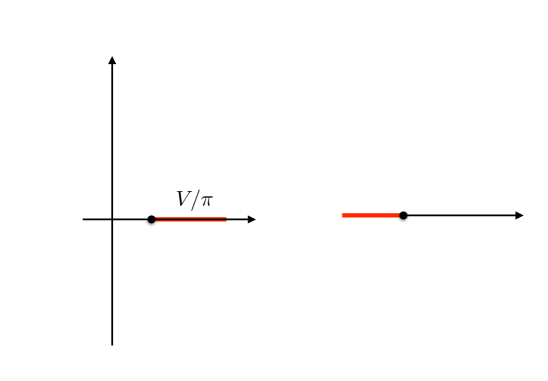
Figure 1. The singularities in the Borel plane for the series $\varphi_{\sigma_{1,2}}(\tau)$.

The structure of singularities in the Borel plane for the formal power series $\varphi_{1,2}(\tau)$ of the $4_{1}$ knot is shown in Fig. 1. Points in each vertical line are $2\pi{\rm i}$ apart, and the two points in the real axis correspond to

$$\iota_{\pm}=\pm\left({V(\sigma_{1})\over 2\pi}-{V(\sigma_{2})\over 2\pi}\right)=\pm{V\over\pi},$$ (69)

where $V$ is defined in (9). Since each singularity in the Borel plane leads to a discontinuity in the Borel resummation, one has the structure of Stokes rays shown in Fig. 2 (where we took into account both series). Note that there is an infinite dense set of rays accumulating towards the imaginary axis.

We already hinted at the end of Section 4.2 that the asymptotic expansion (38) can be upgraded to an exact expression. To do this, one has to upgrade the optimal truncation of $\Phi(\tau)$ to its Borel resummation. Simultaneously we have to promote the matrix of constants appearing in  (38), to a matrix whose entries are power series in $\tilde{q}$ with integer coefficients:

$$\begin{pmatrix}\frac{1}{\sqrt{\tau}}g^{0}_{0}(\tau)\\ \sqrt{\tau}g^{1}_{0}(\tau)\end{pmatrix}=M_{R}(\tilde{q})\,s_{R}(\Phi)(\tau).$$ (70)

The index $R$ labels a sector in the $\tau$-plane, since due to presence of Stokes rays, both the matrix $M_{R}(\tilde{q})$ and the Borel resummed vector $\Phi$ depend on the sector of the $\tau$-plane. In view of the structure of the Stokes rays, convenient sectors to perform the analysis are the angular wedges (i.e., pointed open cones in the complex plane) denoted by $I$, $II$, $III$ and $IV$ in Fig. 2.

It is a challenge to numerically compute the matrix $M_{R}(\tilde{q})$ given only a few hundred terms of $\Phi(\tau)$, since the volume of $4_{1}$ (about $2.02\dots$) is so much smaller than the instanton corrections (appearing at $4\pi^{2}=39.47\dots$). This can be done however, and with 300 terms of $\Phi(\tau)$ it is possible to compute the first twelve terms in the series appearing in $M_{R}(\tilde{q})$. One finds for example, in region $I$,

$$M_{I}(q)=\begin{pmatrix}1-q-2q^{2}-2q^{3}-2q^{4}&-1+2q+3q^{2}+2q^{3}+q^{4}\\ 1-7q-14q^{2}-8q^{3}-2q^{4}&1+10q+15q^{2}-2q^{3}-19q^{4}\end{pmatrix}+O(q^{5}).$$ (71)

Our Conjecture 1 suggests that these $q$-series can be expressed in terms of solutions to the linear $q$-difference equation (11). Indeed, one has, at this order,

$$M_{I}(q)=\begin{pmatrix}G_{0}^{0}(q)&-G_{0}^{0}(q)-G_{-1}^{0}(q)\\ G_{0}^{1}(q)&-G_{0}^{1}(q)-G_{-1}^{1}(q)\end{pmatrix}=W_{-1}(q)^{T}\,\begin{pmatrix}0&-1\\ 1&-1\end{pmatrix}\,.$$ (72)

We conjecture that this is in fact the exact expression for this matrix.

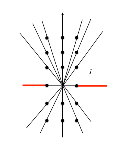
Figure 2. Stokes rays in the $\tau$-plane for $\Phi(\tau)$.

An important consequence of the relation (70) is that, by inverting it, one can express the Borel resummations of $\Phi_{\sigma_{j}}$ for $j=1,2$ in a given sector, in terms of the descendants of the state integral introduced in (4.3), which are holomorphic functions of $\tau$ on $\mathbbm{C}^{\prime}$. Indeed, let us consider the “reduced” descendant

$$\widetilde{\mathcal{I}}_{1,2,\lambda,\mu}(\mathsf{b})=\frac{\tau^{1/2}}{2}G^{1}_{\lambda}(q)G^{0}_{\mu}(\tilde{q})-\frac{\tau^{-1/2}}{2}G^{0}_{\lambda}(q)G^{1}_{\mu}(\tilde{q}).$$ (73)

This differs from the descendant (53) in a manifestly holomorphic factor, so it is holomorphic on $\mathbbm{C}^{\prime}$. Then, one finds, in region $I$,

$$s_{I}(\Phi_{\sigma_{1}})(\tau)=\widetilde{\mathcal{I}}_{1,2,0,0}(\tau)+\widetilde{\mathcal{I}}_{1,2,0,-1,}(\tau),\qquad s_{I}(\Phi_{\sigma_{2}})(\tau)=\widetilde{\mathcal{I}}_{1,2,0,0}(\tau).$$ (74)

This procedure can be done in the other sectors appearing in Fig. 2: one calculates $M_{R}(q)$, express it in terms of fundamental solutions, and represent the Borel resummation $s_{R}(\Phi)$ in terms of holomorphic functions on $\mathbbm{C}^{\prime}$. By comparing the different expressions for the Borel resummations in different sectors, one deduces the Stokes automorphisms relating them, and from a composition of the Stokes automorphisms one deduces the promised $\mathsf{S}$ matrices.

The results for $M_{R}(q)$ are the following:

$$M_{II}(q) =\begin{pmatrix}G_{0}^{0}(q)+G_{-1}^{0}(q)&-G_{0}^{0}(q)\\ -G_{0}^{1}(q)-G_{-1}^{1}(q)&G_{0}^{1}(q)\end{pmatrix}=\begin{pmatrix}1&0\\ 0&-1\end{pmatrix}\,W_{-1}(q)^{T}\,\begin{pmatrix}1&0\\ 1&-1\end{pmatrix},$$ (75)

$$M_{III}(q) =\begin{pmatrix}G_{0}^{0}(q^{-1})+G_{-1}^{0}(q^{-1})&G_{0}^{0}(q^{-1})\\ G_{0}^{1}(q^{-1})+G_{-1}^{1}(q^{-1})&G_{0}^{1}(q^{-1})\end{pmatrix}=W_{-1}(q^{-1})^{T}\,\begin{pmatrix}1&0\\ 1&1\end{pmatrix},$$

$$M_{IV}(q) =\begin{pmatrix}G_{0}^{0}(q^{-1})&G_{0}^{0}(q^{-1})+G_{-1}^{0}(q^{-1})\\ -G_{0}^{1}(q^{-1})&-G_{0}^{1}(q^{-1})-G_{-1}^{1}(q^{-1})\end{pmatrix}=\begin{pmatrix}1&0\\ 0&-1\end{pmatrix}\,W_{-1}(q^{-1})^{T}\,\begin{pmatrix}0&1\\ 1&1\end{pmatrix}\,.$$

From these values one deduces the Stokes automorphisms

$$s_{II}(\Phi) =\mathfrak{S}_{I\rightarrow II}(\tilde{q})s_{I}(\Phi), s_{IV}(\Phi) =\mathfrak{S}_{III\rightarrow IV}(\tilde{q}^{-1})s_{III}(\Phi)$$

$$s_{I}(\Phi) =\mathfrak{S}_{IV\mapsto I}s_{IV}(\Phi), s_{III}(\Phi) =\mathfrak{S}_{II\mapsto III}s_{III}(\Phi),$$ (76)

where

$$\mathfrak{S}_{I\rightarrow II}(q) =M_{II}(q)^{-1}M_{I}(q) \mathfrak{S}_{III\rightarrow IV}(q) =M_{IV}(q^{-1})^{-1}M_{III}(q^{-1})$$ (77a)

$$\mathfrak{S}_{IV\rightarrow I} =M_{I}(q)^{-1}M_{IV}(q) \mathfrak{S}_{II\rightarrow III} =M_{III}(q)^{-1}M_{II}(q)\,.$$ (77b)

and

$$\mathsf{S}^{+}(q)=\mathfrak{S}_{I\rightarrow II}(q)\mathfrak{S}_{IV\rightarrow I},\qquad\mathsf{S}^{-}(q)=\mathfrak{S}_{III\rightarrow IV}(q)\mathfrak{S}_{II\rightarrow III}\,.$$ (78)

Substituting the conjectured values for $M_{R}$ and using symmetry and the orthogonality relations  (15) and (16) one obtains (18a), (18b). In the $q\mapsto 0$ limit the Stokes matrices read

$$\mathsf{S}^{+}(0)=\begin{pmatrix}1&3\\ 0&1\end{pmatrix}\,,\quad\mathsf{S}^{-}(0)=\begin{pmatrix}1&0\\ -3&1\end{pmatrix}.$$ (79)

The off–diagonal entries $\pm 3$ are Stokes constants associated to the singularities $\iota_{\pm}$ on the positive and negative real axis respectively. They agree with the matrix of integers obtained in [GH18],[GZc]. Note that the Stokes matrices $\mathsf{S}^{\pm}(q)$ can also be factorized according to (67) in order to extract all the other Stokes constants. This will be studied in [GGMn20a]. Let us finally note that

$$\mathsf{S}^{+}_{\sigma_{1}\sigma_{1}}(q)=G_{0}^{0}(q)G_{0}^{1}(q)=1-8q-9q^{2}+18q^{3}+46q^{4}+O(q^{5})={\rm Ind}^{\rm rot}_{4_{1}}(q),$$ (80)

in agreement with Conjecture 2 (the fact that $G_{0}^{0}(q)G_{0}^{1}(q)$ equals the rotated index was pointed out in [GZb]).

5.3. The $5_{2}$ knot

The structure of singularities in the Borel plane for the formal power series $\varphi_{\sigma_{j}}(\tau)$ ($j=1,2,3$) of the $5_{2}$ knot is shown in Fig. 3. Points in each vertical line are $2\pi{\rm i}$ are apart, while the six points $\iota_{ij}$ surrounding the origin are given by

$$\iota_{ij}=\frac{V(\sigma_{i})}{2\pi}-\frac{V(\sigma_{j})}{2\pi},\qquad 1\leq i\neq j\leq 3\,,$$ (81)

where $V(\sigma_{i})$ are given in (21). The structure of Stokes rays is shown in Fig. 4. There is also an infinite dense set of rays accumulating towards the imaginary axis.

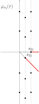
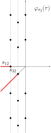
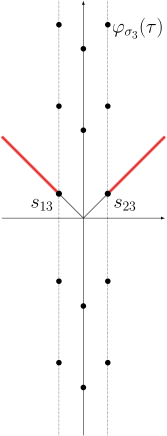
Figure 3. The singularities in the Borel plane for the series $\varphi_{\sigma_{j}}(\tau)$ of the $5_{2}$ knot for $j=1,2,3$.

The $q$-series $H^{\pm}_{k,0}$ for $(k=0,1,2)$, which are analogues of $G^{0}_{0},G^{1}_{0}$ of the $4_{1}$ knot, have similarly interesting radial asymptotics. We use small letters for the corresponding functions, i.e.

$$h_{k}(\tau)=\begin{cases}H^{+}_{k,0}({\rm e}^{2\pi{\rm i}\tau}),\quad&\Im(\tau)>0\\ H^{-}_{k,0}({\rm e}^{-2\pi{\rm i}\tau}),\quad&\Im(\tau)<0\end{cases},\quad k=0,1,2\,.$$ (82)

Then the exact expression of the radial asymptotics reads

$${\rm e}^{3\pi{\rm i}/4}\left(\begin{array}[]{c}\tau^{-1}h_{0}(\tau)\\ h_{1}(\tau)\\ \tau h_{2}(\tau)\end{array}\right)=M_{R}(\tilde{q})s_{R}(\Phi)(\tau),$$ (83)

where the index $R$ labels a sector in the $\tau$-plane. The entries of the matrix $M_{R}(\tilde{q})$ are power series in $\tilde{q}$ in the upper half plane, and power series in $1/\tilde{q}$ in the lower half-plane.

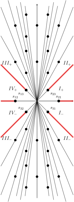
Figure 4. Stokes rays in the $\tau$-plane for $\Phi_{\sigma_{j}}(\tau)$ of the $5_{2}$ knot for $j=1,2,3$. Note that the points $s_{23},s_{31}$ happen to have the same real part, and so do $s_{13},s_{32}$. The dots are not shown in scale for aesthetic purpose.

With more than 200 terms of $\Phi(\tau)$, we are able to compute first few terms in $M_{R}(\tilde{q})$. For instance, in region $I_{+}$ we are able to compute first six terms in each entry of $M_{I_{+}}(\tilde{q})$. We display some of the results here

$$M_{I_{+}}(q)=\begin{pmatrix}-1-q^{2}&2+3q^{2}&1+q+3q^{2}\\ -1+3q+3q^{2}&1-6q-3q^{2}&-q\\ -\frac{5}{6}+5q-\frac{53}{6}q^{2}&-\frac{4}{3}-4q+\frac{77}{2}q^{2}&-\frac{1}{6}+\frac{29}{6}q+\frac{55}{2}q^{2}\end{pmatrix}+O(q^{3}).$$ (84)

Following Conjecture 1, we can express it in terms of solutions to the linear $q$-difference equation (23)

$$M_{I_{+}}(q)=W_{-1}(q)^{T}\begin{pmatrix}0&0&1\\ -1&3&0\\ 0&-1&0\end{pmatrix},$$ (85)

where the Wronskian is defined in (25). Note that this expression is exact. By inverting the matrix $M_{I_{+}}(q)$, we can express the Borel resummation of $\Phi_{\sigma_{j}}$ for $j=1,2,3$ in the sector $I_{+}$ in terms of the descendants of the state integal introduced in Equation (39). Let us again introduce the “reduced” descendant

$$\widetilde{\mathcal{I}}_{\lambda,\mu}(\tau)=\tau H_{2,\lambda}^{+}(q)H_{0,\mu}^{-}(\tilde{q})-2H_{1,\lambda}^{+}(q)H_{1,\mu}^{-}(\tilde{q})+\tau^{-1}H_{0,\lambda}^{+}(q)H_{2,\mu}^{-}(\tilde{q}),$$ (86)

which differs from the descendant (111) in a manifestly holomorphic factor. We find in region $I_{+}$

$$s_{I_{+}}(\Phi)(\tau)=\frac{1}{2}{\rm e}^{3\pi{\rm i}/4}\begin{pmatrix}-1&-1&0\\ 0&-1&0\\ 0&0&1\end{pmatrix}\left(\begin{array}[]{c}\widetilde{\mathcal{I}}_{0,-1}\\ \widetilde{\mathcal{I}}_{0,0}\\ \widetilde{\mathcal{I}}_{0,1}\\ \end{array}\right)(\tau)\,.$$ (87)

In other regions, the results for $M_{R}(q)$ are as follows:

• In the upper half-plane

  $$M_{II_{+}}(q)= W_{-1}(q)^{T}\begin{pmatrix}0&-3&1\\ -1&3&0\\ 0&-1&0\end{pmatrix},$$ (88)

  $$M_{III_{+}}(q)= \begin{pmatrix}1&0&0\\ 0&-1&0\\ 0&0&1\end{pmatrix}W_{-1}(q)^{T}\begin{pmatrix}-3&0&1\\ 3&-1&0\\ -1&0&0\end{pmatrix},$$ (89)

  $$M_{IV_{+}}(q)= \begin{pmatrix}1&0&0\\ 0&-1&0\\ 0&0&1\end{pmatrix}W_{-1}(q)^{T}\begin{pmatrix}0&0&1\\ 3&-1&0\\ -1&0&0\end{pmatrix},\qquad|q|<1.$$ (90)

• In the lower half-plane:

  $$M_{I_{-}}(q)= \begin{pmatrix}1&0&0\\ 0&-1&0\\ 0&0&1\end{pmatrix}W_{-1}(q)^{T}\begin{pmatrix}0&0&1\\ -1&-1&0\\ 0&-1&0\end{pmatrix},$$ (91)

  $$M_{II_{-}}(q)= \begin{pmatrix}1&0&0\\ 0&-1&0\\ 0&0&1\end{pmatrix}W_{-1}(q)^{T}\begin{pmatrix}0&0&1\\ -1&-1&-3\\ 0&-1&0\end{pmatrix},$$ (92)

  $$M_{III_{-}}(q)= W_{-1}(q)^{T}\begin{pmatrix}0&0&1\\ -1&-1&-3\\ -1&0&0\end{pmatrix},$$ (93)

  $$M_{IV_{-}}(q)= W_{-1}(q)^{T}\begin{pmatrix}0&0&1\\ -1&-1&0\\ -1&0&0\end{pmatrix},\qquad|q|>1.$$ (94)

From these values one can deduce the Stokes automorphism, in the anticlockwise direction

$$s_{III_{+}}(\Phi)=\mathfrak{S}_{II_{+}\to III_{+}}(\tilde{q})s_{II_{+}}(\Phi),\quad s_{II_{-}}(\Phi)=\mathfrak{S}_{III_{-}\to II_{-}}(\tilde{q}^{-1})s_{III_{-}}(\Phi),$$

$$s_{II_{+}}(\Phi)=\mathfrak{S}_{I_{+}\to II_{+}}s_{I_{+}}(\Phi),\quad s_{I_{-}}(\Phi)=\mathfrak{S}_{II_{-}\to I_{-}}s_{II_{-}}(\Phi),$$

$$s_{IV_{+}}(\Phi)=\mathfrak{S}_{III_{+}\to IV_{+}}s_{III_{+}}(\Phi),\quad s_{III_{-}}(\Phi)=\mathfrak{S}_{IV_{-}\to III_{-}}s_{IV_{-}}(\Phi),$$

$$s_{I_{+}}(\Phi)=\mathfrak{S}_{I_{-}\to I_{+}}s_{I_{-}}(\Phi),\quad s_{IV_{-}}(\Phi)=\mathfrak{S}_{IV_{+}\to IV_{-}}s_{IV_{+}}(\Phi),$$ (95)

where

$$\mathfrak{S}_{II_{+}\to III_{+}}(q)= \frac{1}{2}\begin{pmatrix}0&-1&0\\ 0&-1&-1\\ 1&-3&0\end{pmatrix}\cdot W_{-1}(q^{-1})\cdot\begin{pmatrix}0&0&1\\ 0&-2&0\\ 1&0&0\end{pmatrix}\cdot W_{-1}(q)\cdot\begin{pmatrix}0&-3&1\\ -1&3&0\\ 0&-1&0\end{pmatrix},$$ (96)

$$\mathfrak{S}^{-1}_{III_{-}\to II_{-}}(q)= \frac{1}{2}\begin{pmatrix}0&-1&0\\ -3&3&-1\\ 1&0&0\end{pmatrix}\cdot W_{-1}(q)\cdot\begin{pmatrix}0&0&1\\ 0&-2&0\\ 1&0&0\end{pmatrix}\cdot W_{-1}(q^{-1})^{T}\cdot\begin{pmatrix}0&0&1\\ -1&-1&-3\\ 0&-1&0\end{pmatrix},$$ (97)

and $\mathfrak{S}_{I_{-}\to I_{+}}$,$\mathfrak{S}_{I_{+}\to II_{+}}$,$\mathfrak{S}_{III_{+}\to IV_{+}}$,$\mathfrak{S}_{IV_{+}\to IV_{-}}$,$\mathfrak{S}_{IV_{-}\to III_{-}}$,$\mathfrak{S}_{II_{-}\to I_{-}}$ are given in (100a),(100b). The matrices $\mathsf{S}^{\pm}(q)$ are simply

$$\mathsf{S}^{+}(q)= \mathfrak{S}_{III_{+}\to IV_{+}}\mathfrak{S}_{II_{+}\to III_{+}}(q)\mathfrak{S}_{I_{+}\to II_{+}}\mathfrak{S}_{I_{-}\to I_{+}},$$ (98)

$$\mathsf{S}^{-}(q)= \mathfrak{S}_{II_{-}\to I_{-}}\mathfrak{S}_{III_{-}\to II_{-}}(q)\mathfrak{S}_{IV_{-}\to III_{-}}\mathfrak{S}_{IV_{+}\to IV_{-}},$$ (99)

and we obtain (29a),(29b).

In the $q\mapsto 0$ limit, the Stokes matrices factorize

$$\mathsf{S}^{+}(0)= \mathfrak{S}_{\sigma_{3},\sigma_{1}}\mathfrak{S}_{\sigma_{3},\sigma_{2}}\mathfrak{S}_{\sigma_{1},\sigma_{2}}=\begin{pmatrix}1&0&0\\ 0&1&0\\ -3&0&1\end{pmatrix}\begin{pmatrix}1&0&0\\ 0&1&0\\ 0&3&1\end{pmatrix}\begin{pmatrix}1&4&0\\ 0&1&0\\ 0&0&1\end{pmatrix},$$ (100a)

$$\mathsf{S}^{-}(0)= \mathfrak{S}_{\sigma_{1},\sigma_{3}}\mathfrak{S}_{\sigma_{2},\sigma_{3}}\mathfrak{S}_{\sigma_{2},\sigma_{1}}=\begin{pmatrix}1&0&3\\ 0&1&0\\ 0&0&1\end{pmatrix}\begin{pmatrix}1&0&0\\ 0&1&-3\\ 0&0&1\end{pmatrix}\begin{pmatrix}1&0&0\\ -4&1&0\\ 0&0&1\end{pmatrix}.$$ (100b)

The non-vanishing off-diagonal entry of $\mathfrak{S}_{\sigma_{i},\sigma_{j}}$ is the Stokes constant associated to the Borel singularity $\iota_{i,j}$. Assembling these Stokes constants in a matrix we obtain

$$\begin{pmatrix}0&4&3\\ -4&0&-3\\ -3&3&0\end{pmatrix}$$ (101)

which is what was found numerically in [GZc, Sec.3.3]. Note that the Stokes matrices $\mathsf{S}^{\pm}(q)$ can also be factorized according to (67) in order to extract all the other Stokes constants. This will be studied in detail in [GGMn20a].

We note that

$$\mathsf{S}^{+}_{\sigma_{1}\sigma_{1}}(q)=2H_{1,0}^{+}(q)H_{1,0}^{-}(q)=1-12q+3q^{2}+74q^{3}+90q^{4}+O(q^{5})={\rm Ind}^{\rm rot}_{5_{2}}(q),$$ (102)

in agreement with Conjecture 2.

6. Open questions

In this paper we have formulated conjectures on the full resurgent structure of quantum knot invariants of hyperbolic knots, and we have presented detailed evidence for the first non-trivial cases, namely the knots $4_{1}$ and $5_{2}$. Although we used complex Chern-Simons theory as a way to motivate our results, and state integrals and asymptotic series as a way to present them, it is clear that a key ingredient that controls the description of the asymptotic series in Borel plane is a pair of linear $q$-difference equations with explicit fundamental solutions. It is natural to ask whether these linear $q$-difference equations are related to those that annihilate the 3D-index, or the colored Jones polynomial of a knot [GL05]. The latter is the famous $\widehat{A}$-polynomial of a knot, whose specialization at $q=1$ is conjectured to essentially coincide with the $A$-polynomial of a knot [Gar04]. It is an interesting question to relate the newly found linear $q$-difference equations with the $\widehat{A}$-polynomial of a knot.

One could also consider deformations by an arbitrary holonomy around the knot, which will be explored in [GGMn20a]. In this case, the resulting perturbative series depend on a parameter $x$ (see e.g. [DGLZ09]) that plays the role of a Jacobi variable and one could calculate the Stokes constants in this extended setting. This might make clearer the relation to the $A$-polynomial and its quantization.

Another interesting question is whether the Stokes constants we compute, which are closely related to BPS counting, can be obtained with techniques similar to those of [GMN13], i.e. by doing WKB analysis on the algebraic curve defined by the $A$-polynomial, or some variant thereof.

Finally, we would like to point out that towers of singularities similar to those studied here appear in the Borel plane of topological string partition functions, see e.g. [PS10, CSMnS17]. Understanding the Stokes constants of these singularities in topological string theory would probably lead to fascinating mathematics and to connections with BPS state counting in string theory.

Appendix A $q$-series associated with the $5_{2}$ knot

A.1. The state integral of the $5_{2}$ knot

We now consider the case of $(A,B)=(2,3)$, i.e., the state integral $\mathcal{I}_{2,3,\lambda,\mu}(\mathsf{b})$. The data we need to present our result are

$$F_{2,3,\lambda}(q,x)=\sum_{n=0}^{\infty}\frac{q^{n(n+1)+n\lambda}}{(q;q)_{n}^{3}}x^{n},$$ (103)

$$\widetilde{F}_{2,3,\mu}(\tilde{q},\tilde{x})=\sum_{n=0}^{\infty}(-1)^{n}\frac{\tilde{q}^{\frac{1}{2}n(n+1)+n\mu}}{(\tilde{q};\tilde{q})_{n}^{3}}\tilde{x}^{n},$$ (104)

as well as the operator

$$P_{2,3,\lambda,\mu}= -\frac{1}{2\pi{\rm i}}+(1+2\delta-3\delta_{1}+\lambda)(\frac{1}{2}+\tilde{\delta}-3\tilde{\delta}_{1}+\mu)$$ (105)

$$-\frac{\mathsf{b}^{2}}{2}((1+2\delta-3\delta_{1}+\lambda)^{2}-3\delta_{2})$$ (106)

$$-\frac{\mathsf{b}^{-2}}{2}((\frac{1}{2}+\tilde{\delta}-3\tilde{\delta}_{1}+\mu)^{2}-\frac{1}{4}-3\tilde{\delta}_{2}+6\,E_{2}^{(0)}(\tilde{q})).$$ (107)

Using the observation that

$$-\frac{1}{2\pi{\rm i}}=\frac{1}{12}\left(\tau E_{2}(\tau)-\tau^{-1}E_{2}(-1/\tau)\right)$$ (108)

as well as

$$E_{2}(\tau)=1-24\sum_{s=1}^{\infty}\frac{q^{s}}{(1-q^{s})^{2}}=1-24E_{2}^{(0)}(q),$$ (109)

the final result can be written as ($\tau=\mathsf{b}^{2}$ in the upper half-plane)

$$\mathcal{I}_{2,3,\lambda,\mu}(\mathsf{b}) =(-1)^{\lambda-\mu}e^{\frac{\pi{\rm i}}{4}}q^{\frac{\lambda}{2}}\tilde{q}^{\frac{\mu}{2}}\left(\frac{q}{\tilde{q}}\right)^{\frac{1}{8}}\times$$ (110)

$$\left(-\frac{\tau}{2}H_{2,\lambda}^{+}(q)H_{0,\mu}^{-}(\tilde{q})+H_{1,\lambda}^{+}(q)H_{1,\mu}^{-}(\tilde{q})-\frac{\tau^{-1}}{2}H_{0,\lambda}^{+}(q)H_{2,\mu}^{-}(\tilde{q})\right).$$ (111)

Here

$$H_{j,\lambda}^{+}(q)=\sum_{n=0}^{\infty}p_{n,\lambda}^{(j)}(q)t_{n,\lambda}(q),\quad H_{j,\mu}^{-}(\tilde{q})=\sum_{n=0}^{\infty}P_{n,\mu}^{(j)}(\tilde{q})T_{n,\mu}(\tilde{q}),\qquad(j=0,1,2)\,,$$ (112)

where $t_{n,\lambda}(q),T_{n,\mu}(\tilde{q})$ are coefficients of $F_{2,3,\lambda}(q,x),\widetilde{F}_{2,3,\mu}(\tilde{q},\tilde{x})$ as series of $x,\tilde{x}$,

$$t_{n,\lambda}(q)=\frac{q^{n(n+1)+n\lambda}}{(q;q)_{n}^{3}},$$ (113)

$$T_{n,\mu}(\tilde{q})=(-1)^{n}\frac{\tilde{q}^{\frac{1}{2}n(n+1)+n\mu}}{(\tilde{q};\tilde{q})_{n}^{3}},$$ (114)

while $p_{n,\lambda}^{(j)}(q),P_{n,\mu}^{(j)}(\tilde{q})$ result from applying the operator $P_{2,3,\lambda,\mu}$, i.e.

$$p_{n,\lambda}^{(0)}(q)=1,$$ (115)

$$p_{n,\lambda}^{(1)}(q)=1+2n-3E_{1}^{(n)}(q)+\lambda,$$ (116)

$$p_{n,\lambda}^{(2)}(q)=\left(p_{n,\lambda}^{(1)}(q)\right)^{2}-\frac{1}{6}-3E_{2}^{(n)}(q)+4E_{2}^{(0)}(q),$$ (117)

as well as

$$P_{n,\mu}^{(0)}(\tilde{q})=1,$$ (118)

$$P_{n,\mu}^{(1)}(\tilde{q})=\frac{1}{2}+n-3E_{1}^{(n)}(\tilde{q})+\mu,$$ (119)

$$P_{n,\mu}^{(2)}(\tilde{q})=\left(P_{n,\mu}^{(1)}(\tilde{q})\right)^{2}-\frac{1}{12}-3E_{2}^{(n)}(\tilde{q})+2E_{2}^{(0)}(\tilde{q}).$$ (120)

The $q$-series $H_{j,\lambda}^{+}(q)$ and $H_{j,\mu}^{-}(q)$ for $j=0,1,2$ are exactly those that appear in Equation (25). A few coefficients of the above series are given by

$$H_{0,-1}^{+}(q)= 1+q+3q^{2}+6q^{3}+11q^{4}+18q^{5}+O(q^{6}),$$ (121)

$$H_{1,-1}^{+}(q)= -q+3q^{3}+3q^{4}+3q^{5}+O(q^{6}),$$

$$H_{2,-1}^{+}(q)= -\frac{1}{6}+\frac{29}{6}q+\frac{55}{2}q^{2}+72q^{3}+\frac{895}{6}q^{4}+270q^{5}+O(q^{6}),$$

$$H_{0,-1}^{-}(q)= -2q-3q^{2}-2q^{3}+q^{4}+9q^{5}+O(q^{6}),$$

$$H_{1,-1}^{-}(q)= -1-3q-\frac{3}{2}q^{2}+12q^{3}+\frac{69}{2}q^{4}+\frac{153}{2}q^{5}+O(q^{6}),$$

$$H_{2,-1}^{-}(q)= \frac{5}{3}q+\frac{27}{2}q^{2}+\frac{143}{3}q^{3}+\frac{541}{6}q^{4}+\frac{263}{2}q^{5}+O(q^{6}).$$

$$H_{0,0}^{+}(q)= 1+q^{2}+3q^{3}+6q^{4}+10q^{5}+O(q^{6}),$$ (122)

$$H_{1,0}^{+}(q)= 1-3q-3q^{2}+3q^{3}+6q^{4}+12q^{5}+O(q^{6}),$$

$$H_{2,0}^{+}(q)= \frac{5}{6}-5q+\frac{53}{6}q^{2}+\frac{117}{2}q^{3}+117q^{4}+\frac{601}{3}q^{5}+O(q^{6}),$$

$$H_{0,0}^{-}(q)= 1-q-3q^{2}-5q^{3}-7q^{4}-6q^{5}+O(q^{6}),$$

$$H_{1,0}^{-}(q)= \frac{1}{2}-\frac{9}{2}q-\frac{21}{2}q^{2}-\frac{19}{2}q^{3}-\frac{9}{2}q^{4}+27q^{5}+O(q^{6}),$$

$$H_{2,0}^{-}(q)= \frac{1}{6}-\frac{37}{6}q-\frac{17}{2}q^{2}+\frac{115}{6}q^{3}+\frac{389}{6}q^{4}+181q^{5}+O(q^{6}).$$

$$H_{0,1}^{+}(q)= 1+q^{3}+3q^{4}+6q^{5}+O(q^{6}),$$ (123)

$$H_{1,1}^{+}(q)= 2-3q-6q^{2}-2q^{3}+3q^{4}+15q^{5}+O(q^{6}),$$

$$H_{2,1}^{+}(q)= \frac{23}{6}-11q-12q^{2}+\frac{191}{6}q^{3}+\frac{189}{2}q^{4}+200q^{5}+O(q^{6}),$$

$$H_{0,1}^{-}(q)= 1-q^{2}-3q^{3}-6q^{4}-9q^{5}+O(q^{6}),$$

$$H_{1,1}^{-}(q)= \frac{3}{2}-3q-\frac{17}{2}q^{2}-\frac{27}{2}q^{3}-21q^{4}-\frac{31}{2}q^{5}+O(q^{6}),$$

$$H_{2,1}^{-}(q)= \frac{13}{6}-10q-\frac{109}{6}q^{2}-\frac{13}{2}q^{3}+7q^{4}+\frac{173}{2}q^{5}+O(q^{6}).$$

A.2. The symmetry $q\leftrightarrow q^{-1}$

We now discuss the symmetry $q\mapsto q^{-1}$. It is easy to see that the above $q$-series $H_{j,\lambda}^{\pm}(q)$ are well-defined holomorphic functions when $q$ is either inside or outside the unit disk. Extended this way, we claim that

$$H_{j,\lambda}^{+}(q)=(-1)^{j}H_{j,-\lambda}^{-}(1/q),\qquad(q\in\mathbbm{C},\,\,|q|\neq 1)\,.$$ (124)

This follows from the easy observation

$$t_{n,\lambda}(q)=T_{n,-\lambda}(1/q)\,$$ (125)

and the less trivial symmetry

$$E_{1}(\tau)=-E_{1}(-\tau),\quad E_{2}(\tau)=-E_{2}(-\tau)$$ (126)

(see for instance [BC13] for the first and [CMZ18] for the second), where $E_{1},E_{2}$ are related to $E_{1}^{(0)},E_{2}^{(0)}$ by

$$E_{1}(\tau) =1-4\sum_{n\geq 1}\frac{q^{n}}{1-q^{n}}=1-4E_{1}^{(0)}(q),$$ (127)

$$E_{2}(\tau) =1-24\sum_{n\geq 1}\frac{q^{n}}{(1-q^{n})^{2}}=1-24E_{2}^{(0)}(q)\,.$$ (128)

Equations (125) and (126) and induction on the exponent $n$ of $E_{1}^{(n)},E_{2}^{(n)}$ imply that

$$p_{n,\lambda}^{(k)}(q)=(-1)^{k}P_{n,-\lambda}^{(k)}(1/q)$$ (129)

for all $n$, and this concludes the proof of Equation (124).

The above conclusions hold not only for the state integral with $(A,B)=(2,3)$ or $(A,B)=(1,2)$, but for the case of arbitrary integers $A$ and $B$ with $B>A>0$.

References

- [ABS19] Inês Aniceto, Gökçe Başar, and Ricardo Schiappa, A primer on resurgent transseries and their asymptotics, Phys. Rep. 809 (2019), 1–135.
- [AK14] Jorgen Ellegaard Andersen and Rinat Kashaev, A TQFT from Quantum Teichmüller theory, Comm. Math. Phys. 330 (2014), no. 3, 887–934.
- [BC13] Sandro Bettin and Brian Conrey, Period functions and cotangent sums, Algebra Number Theory 7 (2013), no. 1, 215–242.
- [BDP14] Christopher Beem, Tudor Dimofte, and Sara Pasquetti, Holomorphic blocks in three dimensions, J. High Energy Phys. (2014), no. 12, 177, front matter+118.
- [CC01] O. Costin and R. D. Costin, On the formation of singularities of solutions of nonlinear differential systems in antistokes directions, Invent. Math. 145 (2001), no. 3, 425–485.
- [CG11] Ovidiu Costin and Stavros Garoufalidis, Resurgence of the Kontsevich-Zagier series, Ann. Inst. Fourier (Grenoble) 61 (2011), no. 3, 1225–1258.
- [CMHR+07] E. Caliceti, M. Meyer-Hermann, P. Ribeca, A. Surzhykov, and U. D. Jentschura, From useful algorithms for slowly convergent series to physical predictions based on divergent perturbative expansions, Phys. Rep. 446 (2007), no. 1-3, 1–96.
- [CMZ18] Dawei Chen, Martin Möller, and Don Zagier, Quasimodularity and large genus limits of Siegel-Veech constants, J. Amer. Math. Soc. 31 (2018), no. 4, 1059–1163.
- [CSMnS17] Ricardo Couso-Santamaría, Marcos Mariño, and Ricardo Schiappa, Resurgence matches quantization, J. Phys. A 50 (2017), no. 14, 145402, 34.
- [DG13] Tudor Dimofte and Stavros Garoufalidis, The quantum content of the gluing equations, Geom. Topol. 17 (2013), no. 3, 1253–1315.
- [DG18] by same author, Quantum modularity and complex Chern-Simons theory, Commun. Number Theory Phys. 12 (2018), no. 1, 1–52.
- [DGG13] Tudor Dimofte, Davide Gaiotto, and Sergei Gukov, 3-manifolds and 3d indices, Adv. Theor. Math. Phys. 17 (2013), no. 5, 975–1076.
- [DGG14] by same author, Gauge theories labelled by three-manifolds, Comm. Math. Phys. 325 (2014), no. 2, 367–419.
- [DGLZ09] Tudor Dimofte, Sergei Gukov, Jonatan Lenells, and Don Zagier, Exact results for perturbative Chern-Simons theory with complex gauge group, Commun. Number Theory Phys. 3 (2009), no. 2, 363–443.
- [Fad95] L. D. Faddeev, Discrete Heisenberg-Weyl group and modular group, Lett. Math. Phys. 34 (1995), no. 3, 249–254.
- [FK94] Ludwig Faddeev and Rinat Kashaev, Quantum dilogarithm, Modern Phys. Lett. A 9 (1994), no. 5, 427–434.
- [Gar04] Stavros Garoufalidis, On the characteristic and deformation varieties of a knot, Proceedings of the Casson Fest, Geom. Topol. Monogr., vol. 7, Geom. Topol. Publ., Coventry, 2004, pp. 291–309 (electronic).
- [Gar08] Stavros Garoufalidis, Chern-Simons theory, analytic continuation and arithmetic, Acta Math. Vietnam. 33 (2008), no. 3, 335–362.
- [GGMn20a] Stavros Garoufalidis, Jie Gu, and Marcos Mariño, Peacock patterns and resurgence in complex Chern-Simons theory, 2012.00062.
- [GGMn20b] Alba Grassi, Jie Gu, and Marcos Mariño, Non-perturbative approaches to the quantum Seiberg-Witten curve, JHEP 07 (2020), 106, 1908.07065.
- [GH18] Dongmin Gang and Yasuyuki Hatsuda, S-duality resurgence in Chern-Simons theory, J. High Energy Phys. (2018), no. 7, 053, front matter+23.
- [GK17] Stavros Garoufalidis and Rinat Kashaev, From state integrals to -series, Math. Res. Lett. 24 (2017), no. 3, 781–801.
- [GL05] Stavros Garoufalidis and Thang T. Q. Lê, The colored Jones function is -holonomic, Geom. Topol. 9 (2005), 1253–1293 (electronic).
- [GLMn08] Stavros Garoufalidis, Thang T. Q. Lê, and Marcos Mariño, Analyticity of the free energy of a closed 3-manifold, SIGMA Symmetry Integrability Geom. Methods Appl. 4 (2008), Paper 080, 20.
- [GMN10] Davide Gaiotto, Gregory W. Moore, and Andrew Neitzke, Four-dimensional wall-crossing via three-dimensional field theory, Comm. Math. Phys. 299 (2010), no. 1, 163–224.
- [GMN13] by same author, Wall-crossing, Hitchin systems, and the WKB approximation, Adv. Math. 234 (2013), 239–403.
- [GMnP] Sergei Gukov, Marcos Mariño, and Pavel Putrov, Resurgence in complex Chern-Simons theory, arXiv:1605.07615, Preprint 2016.
- [Guk05] Sergei Gukov, Three-dimensional quantum gravity, Chern-Simons theory, and the A-polynomial, Comm. Math. Phys. 255 (2005), no. 3, 577–627.
- [GZa] Stavros Garoufalidis and Don Zagier, Asymptotics of Nahm sums at roots of unity, With an appendix by Sander Zwegers.
- [GZb] by same author, Knots and their related -series, Preprint 2020.
- [GZc] by same author, Knots, perturbative series and quantum modularity, Preprint 2020.
- [Hik07] Kazuhiro Hikami, Generalized volume conjecture and the -polynomials: the Neumann-Zagier potential function as a classical limit of the partition function, J. Geom. Phys. 57 (2007), no. 9, 1895–1940.
- [IMnS19] Katsushi Ito, Marcos Mariño, and Hongfei Shu, TBA equations and resurgent quantum mechanics, J. High Energy Phys. (2019), no. 1, 228, front matter+44.
- [Kas95] Rinat Kashaev, A link invariant from quantum dilogarithm, Modern Phys. Lett. A 10 (1995), no. 19, 1409–1418.
- [Kas97] R. M. Kashaev, The hyperbolic volume of knots from the quantum dilogarithm, Lett. Math. Phys. 39 (1997), no. 3, 269–275.
- [Kon20] Maxim Kontsevich, Exponential integrals, Lefschetz thimbles and linear resurgence, June 2020, ReNewQuantum seminar, https://renewquantum.eu/docs/Lecture_slides_MaximKontsevich_June2020.pdf, 2020.
- [KS11] Maxim Kontsevich and Yan Soibelman, Cohomological Hall algebra, exponential Hodge structures and motivic Donaldson-Thomas invariants, Commun. Number Theory Phys. 5 (2011), no. 2, 231–352.
- [KS20] by same author, Analyticity and resurgence in wall-crossing formulas, 2005.10651.
- [Mn19] Marcos Mariño, From resurgence to BPS states, talk given at the conference Strings 2019, Brussels, https://livestream.com/accounts/7777696/events/8742238/videos/193704304, 2019.
- [MS16] Claude Mitschi and David Sauzin, Divergent series, summability and resurgence. I, Lecture Notes in Mathematics, vol. 2153, Springer, 2016.
- [PS10] Sara Pasquetti and Ricardo Schiappa, Borel and Stokes nonperturbative phenomena in topological string theory and matrix models, Ann. Henri Poincaré 11 (2010), no. 3, 351–431.
- [Vor83] A. Voros, The return of the quartic oscillator: the complex WKB method, Ann. Inst. H. Poincaré Sect. A (N.S.) 39 (1983), no. 3, 211–338.