Resummation and simulation of soft gluon effects beyond leading colour

Abstract

We present first results of resumming soft gluon effects in a simulation of high energy collisions beyond the leading-colour approximation. We work to all orders in QCD perturbation theory using a new parton branching algorithm. This amplitude evolution algorithm resembles a parton shower that is able to systematically include colour-suppressed terms. We find that colour suppressed terms can significantly contribute to jet veto cross sections.

Introduction – We present first results from a new Monte Carlo code, CVolver, that simulates high-energy particle collisions . Our analysis here is based upon simulated two-jet events and our goal is to improve on the accuracy of existing simulations Bähr et al. (2008); Bellm et al. (2016); Sjöstrand et al. (2015); Bothmann et al. (2019) by including colour correlations beyond the leading-colour approximation. To do so we pursue a new paradigm of evolution at the amplitude level in place of the traditional probabilistic algorithms (see also Nagy and Soper (2012, 2015); Martínez et al. (2018); Forshaw et al. (2019); Nagy and Soper (2019a, b)). In the next section we introduce the theoretical framework, with particular emphasis on our treatment of colour. In the following section, we present results for the cross section for the production of a two-jet system with a restriction on the amount of radiation lying in some angular region outside of the jets. This process is sensitive to wide-angle, soft-gluon emission and thus provides a good test of the framework. We observe significant deviations from the leading-colour approximation.

Summing soft-gluon effects – Particle collisions involving coloured particles and a large transfer of momentum, $Q$, are computable using perturbative QCD. However, fixed-order perturbation theory is often insufficient due to the presence of large logarithms that compensate the smallness of the perturbative coupling, $\alpha_{s}$. In other words, there exist terms of order $\alpha_{s}^{n}L^{m}$ where $L$ is some large logarithm and $m\leq 2n$. Large logarithms can arise if gluons are emitted with a low energy compared to the large momentum transfer, and if the observable is sensitive to those emissions. We refer to these as soft-gluon logarithms and, in Martínez et al. (2018), we presented an iterative algorithm for summing them to all orders in perturbation theory for general short-distance scattering processes. In this paper, we will sum the most important of these logarithms, though the framework is general enough to go beyond this ‘leading logarithmic approximation’. The formalism can be extended to also include logarithms of collinear origin Forshaw et al. (2019, 2020). The differential cross section for $n$ soft-gluon emissions can be written

$$\text{d}\sigma_{n} =\text{Tr}\,\mathbf{A}_{n}\,\text{d}\Pi_{n}~{},$$ (1)

where the operators $\mathbf{A}_{n}$ satisfy the recurrence relation

$$\mathbf{A}_{n}(E)=\mathbf{V}_{E,E_{n}}\mathbf{D}_{n}^{\mu}\;\mathbf{A}_{n-1}(E_{n})\;\mathbf{D}_{n\mu}^{\dagger}\mathbf{V}_{E,E_{n}}^{\dagger}\,\Theta(E\leq E_{n}),$$

(2)

where $\Theta(E\leq E_{n})$ is the Heaviside function. The virtual-gluon (Sudakov) operator sums over all single-gluon exchanges between pairs of partons. For two-jet production off a colour singlet (e.g. $V\to q\bar{q}$ or $H\to gg$) it is given by

$${\mathbf{V}}_{a,b} = \exp\Bigg{[}-\frac{\alpha_{s}}{\pi}\ln\left(\frac{b}{a}\right)\;\sum_{i<j}(-\mathbf{T}_{i}\cdot\mathbf{T}_{j})\,$$

$$\times\int\frac{\text{d}\Omega}{4\pi}\frac{n_{i}\cdot n_{j}}{(n_{i}\cdot n)\;(n_{j}\cdot n)}\Bigg{]}~{},$$

where $n_{i}$ is a light-like vector whose spatial part is the unit vector in the direction that particle $i$ travels. The integral is over the direction of the light-like vector $n$ and, for now, we take $\alpha_{s}$ to be fixed. The real emission operator and phase-space factor are

$$\mathbf{D}_{i}^{\mu} =\sum_{j}\mathbf{T}_{j}\;E_{i}\frac{p_{j}^{\mu}}{p_{j}\cdot q_{i}}~{}~{}~{}\text{and}$$

$$\text{d}\Pi_{n} =\prod_{i=1}^{n}\left(-\frac{\alpha_{s}}{\pi}\frac{\text{d}E_{i}}{E_{i}}\frac{\text{d}\Omega_{i}}{4\pi}\right)~{}.$$ (4)

Note that the sum over partons in the definitions of $\mathbf{V}_{a,b}$ and $\mathbf{D}_{i}^{\mu}$ is context-specific, i.e. it runs over all prior soft-gluon emissions in addition to the partons in the original hard scattering. The colour charge operator, $\mathbf{T}_{j}$, is also in a context-specific representation of SU(3)_c. Soft-gluon evolution proceeds iteratively starting from a hard-scattering operator, $\mathbf{H}=|\mathcal{M}\rangle\langle\mathcal{M}|$ with $\mathbf{A}_{0}(E)=\mathbf{V}_{E,Q}\,\mathbf{H}\,\mathbf{V}_{E,Q}^{\dagger}$. A general observable, $\Sigma$, can be computed using

$$\Sigma(\mu) = \int\sum_{n}~{}\text{d}\sigma_{n}\,u_{n}(k_{1},k_{2},\cdots,k_{n})~{},$$ (5)

where the $u_{n}$ are the observable dependent measurement functions and the $k_{i}$ are soft-gluon momenta. We suppress the dependence on the hard partons and integration over their phase space. Although we assume energy ordering, this is not essential and the algorithm can readily be adapted to account for a different ordering variable. We should take the limit $\mu\to 0$ in Eq. (5), though it is also correct to put $\mu=Q_{0}$ if the observable is fully inclusive over gluon emissions with $E<Q_{0}$.

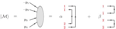
Figure 1: An example of an amplitude decomposed in the colour flow basis.

This iterative form of the algorithm is well suited to a Monte Carlo implementation. The kinematic part of the evolution is diagonal and does not pose any new problems. The main challenge is to account for the independent colour evolution in the amplitude and the conjugate amplitude. To do this we use the colour-flow basis, which is illustrated in the case where the hard scattering process is $q\bar{q}\to q\bar{q}$ in Fig. 1. We choose to draw all particles in the amplitude as heading off to the left and negative momenta indicate incoming particles. The particle with incoming momentum $p_{1}$ is an anti-quark, that with incoming momentum $p_{2}$ is a quark whilst $p_{3}$ and $p_{4}$ label an outgoing quark and an outgoing anti-quark respectively. In the colour-flow basis, quarks and anti-quarks are represented by colour and anti-colour lines (an incoming quark is represented by an anti-colour line), whilst gluons are represented by a pair of colour and anti-colour lines. A basis vector in the colour space is then represented by stating how the colour and anti-colour lines are connected. We see this on the right-hand side of Fig. 1. In the first term, the incoming anti-quark is colour connected to the outgoing anti-quark and the incoming quark is colour connected to the outgoing quark. The second term is the only other possibility for two colour lines and corresponds to the case where the incoming quark is colour connected to the incoming anti-quark. Our convention is to write amplitudes such that Fig. 1 corresponds to

$$\ket{\mathcal{M}}=\alpha\ket{21}+\beta\ket{12}~{}.$$ (6)

A general state consisting of $n$ colour lines has a basis of dimension $n!$ corresponding to all possible permutations of the numbers $(1,2,\cdots,n)$. We normalize the basis vectors so that

$$\braket{\alpha}{\beta}=N_{c}^{n-\#(\alpha,\beta)},$$ (7)

where $\#(\alpha,\beta)$ is the minimum number of pairwise swaps by which the permutations $\alpha$ and $\beta$ differ, e.g. $\braket{12}{12}=N_{c}^{2}$ and $\braket{12}{21}=N_{c}$. This basis is over-complete and not orthogonal but is very simple to implement and provides excellent opportunities for importance sampling. We introduce a dual basis, $|\alpha]$, such that $\bra{\alpha}\beta]=[\alpha\ket{\beta}=\delta_{\alpha\beta}$, where $\delta_{\alpha\beta}$ is unity if the two permutations are equal and zero otherwise. Also, $\sum_{\alpha}\ket{\alpha}[\alpha|=\mathbf{1}$. The trace in Eq. (1) is then computed using

$$\text{Tr}\,\mathbf{A}_{n}=\sum_{\sigma,\tau}[\tau|\mathbf{A}_{n}|\sigma]\braket{\sigma}{\tau}~{}.$$ (8)

Fig. 2 illustrates how we Monte Carlo over intermediate colour states by inserting the unit operator between successive real emission and virtual correction operators.

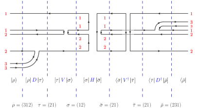
Figure 2: One contribution to the $\mathbf{A}_{1}$ operator, starting from the hard scattering illustrated in Fig. 1. It corresponds to single gluon emission with two virtual gluon exchanges. The vertical dotted lines are to help identify the intermediate colour states. The algorithm works iteratively outwards, starting from the hard process in the middle and multiplying matrix elements as it goes.

We select initial colour flows, $\sigma$ and $\bar{\sigma}$, and compute the corresponding hard scattering matrix $[\sigma|\mathbf{H}|\bar{\sigma}]$. Then we choose the momentum of the first real emission and, in anticipation of inserting Sudakov operators that act on the amplitude and the conjugate (they evolve from the hard scale $Q$ down to the energy of the emitted gluon, $E_{1}$), we choose two new colour flows, $\tau$ and $\bar{\tau}$, from the set of all possible colour flows that can be accessed after the action of a Sudakov operator (see below). We then multiply the original hard scattering matrix element by the corresponding Sudakov matrix elements. The colour states $\rho$ and $\bar{\rho}$ are chosen next, from the set of all possible permutations accessible after the emission of a gluon and these are used to deduce the corresponding real emission matrix elements. This whole process repeats until the evolution terminates and the final product of matrix elements must be further multiplied by the scalar product matrix, $\braket{\sigma_{m}}{\bar{\sigma}_{m}}$, where $m$ labels the final colour flows. This induces a $1/N_{c}$ suppression factor for every swap by which the final permutations $\sigma_{m}$ and $\bar{\sigma}_{m}$ differ.

Eq. (2) can be re-written explicitly in terms of matrix elements such that one step in the evolution is determined by

$$M_{\rho\bar{\rho}}(E)=-\frac{\alpha_{s}}{\pi} \frac{\text{d}E}{E}\frac{\text{d}\Omega}{4\pi}\,\sum_{\begin{subarray}{c}\tau,\sigma\\ \bar{\tau},\bar{\sigma}\end{subarray}}[\rho|\mathbf{D}_{E}\ket{\tau}[\tau|\mathbf{V}_{E,E^{\prime}}\ket{\sigma}$$

$$M_{\sigma\bar{\sigma}}(E^{\prime})\bra{\bar{\sigma}}\mathbf{V}^{\dagger}_{E,E^{\prime}}|\bar{\tau}]\bra{\bar{\tau}}\mathbf{D}_{E}^{\dagger}|\bar{\rho}],$$ (9)

where $E$ is the energy of the latest emission and $E^{\prime}$ is the previous energy. This expression is the core of our implementation and it provides a map from a pair of colour flows $(\sigma,\bar{\sigma})$ to the pair $(\rho,\bar{\rho})$.

Calculating the effect of real emission matrix elements and virtual gluon corrections involves computing matrix elements $[\tau|\mathbf{T}_{i}\ket{\sigma}$ and $[\tau|\mathbf{T}_{i}\cdot\mathbf{T}_{j}\ket{\sigma}$. Explicit expressions for these are presented in Martínez et al. (2018). For the real emissions, the calculations are simplified since the real emission operator can either: (a) add a new colour line without changing any of the existing colour connections or (b) add a new colour line and then make a single swap. In the case that the gluon is emitted off a colour line this swap connects the colour of the emitted gluon to the anti-colour partner of the emitter (and likewise if the gluon is emitted off an anti-colour line). Taken together, a real emission in the amplitude and the conjugate amplitude only changes the number of swaps by which the two colour flows (in the amplitude and conjugate) differ by at most two. Specifically, $0\leq\#(\sigma_{n+1},\tau_{n+1})-\#(\sigma_{n},\tau_{n})\leq 2$. This means that real emissions never bring the two colour flows ‘closer together’. ‘Singlet’ gluons, as emitted in case (a), are subleading in colour and inert from the point of view of the subsequent evolution. The simplicity of the real emissions means we do not need to make any approximation when computing them.

The main challenge is to compute the Sudakov matrix elements, $[\tau|\mathbf{V}\ket{\sigma}$, which involves the exponentiation of a possibly large colour matrix. The evaluation can be considerably simplified if we are prepared to sum terms accurate only to order $1/N_{c}^{d}$, where $d$ is a positive integer, while keeping the leading diagonal terms proportional to $(\alpha_{s}N_{c})^{n}$ to all orders $n$. Choosing larger values of $d$ will lead to more accurate results that take a longer time to compute. To do this we use the result presented in Plätzer (2014):

$$[\tau|\mathbf{V}\ket{\sigma} \approx \delta_{\tau\sigma}R(\{\sigma\})+\sum_{l=1}^{d}\left(-\frac{1}{N_{c}}\right)^{l}\sum_{\sigma_{0},\sigma_{1},\cdots\sigma_{l}}\delta_{\tau\sigma_{0}}\delta_{\sigma_{l}\sigma}$$ (10)

$$\times\prod_{\alpha=0}^{l-1}\Sigma_{\sigma_{\alpha}\sigma_{\alpha+1}}\,R(\{\sigma_{0},\sigma_{1},\cdots,\sigma_{l}\})~{}.$$

The anomalous dimension matrix elements are

$$[\tau|\ln\mathbf{V}\ket{\sigma}=\left(-N_{c}\,\Gamma_{\sigma}+\frac{\rho}{N_{c}}\right)\delta_{\tau\sigma}+\Sigma_{\tau\sigma}~{}.$$ (11)

Explicit expressions for $\Gamma_{\sigma}$, $\rho$ and $\Sigma_{\sigma\tau}$ can be computed using the results presented in Plätzer (2014); Martínez et al. (2018). Note that the off-diagonal contribution, $\Sigma_{\tau\sigma}$, is only non-zero if $\#(\sigma,\tau)=1$. In other words, each virtual gluon exchange can either leave a colour flow unchanged or induce a single swap. Exponentiating this to produce the Sudakov operator generates the possibility of many swaps but this can be managed since each swap comes at the price of a factor $1/N_{c}$. This is what allows us to truncate the sum in Eq. (10) at a small value of $d$. We refer to $d=0$ as our leading colour virtuals (LC_V) approximation and $d=1$ as next-to-leading (NLC_V) etc. The kinematic functions $R$ appearing in Eq. (10) are also listed in Plätzer (2014). In the case $d=0$, we only need

$$R(\{\sigma\})=e^{-N_{c}\Gamma_{\sigma}^{\prime}}~{},$$ (12)

where $\Gamma^{\prime}_{\sigma}=\Gamma_{\sigma}-\rho/N_{c}^{2}$. Keeping only this term generates the leading colour approximation, improved by summing the colour-diagonal subleading parts . For $d=1$ we also need

$$R(\{\tau,\sigma\}) =\frac{e^{-N_{c}\Gamma^{\prime}_{\tau}}-e^{-N_{c}\Gamma^{\prime}_{\sigma}}}{\Gamma^{\prime}_{\tau}-\Gamma^{\prime}_{\sigma}}$$ (13)

so that the NLC_V Sudakov matrix elements are

$$[\tau|\mathbf{V}\ket{\sigma}=\delta_{\tau\sigma}e^{-N_{c}\Gamma^{\prime}_{\sigma}}-\frac{1}{N_{c}}\Sigma_{\tau\sigma}R(\{\tau,\sigma\}).$$ (14)

Notice that our N^dLC_V approximation involves at most $d$ swaps for each application of the Sudakov operator, which makes the task of Monte Carloing over accessible colour states tractable. It should be emphasised that since we treat the real emissions, the scalar product matrix and the diagonal part of the anomalous dimension matrix without any approximation, our leading-colour approximation goes well beyond summing only the strictly leading ($m=0$) terms in an expansion in $(N_{c}\alpha_{s})^{n}/N_{c}^{m}$, see also Holguin et al. (2020) for a recent discussion.

One stringent test of the algorithm is that it should correctly handle the cancellation of collinear singular terms. We deal with the collinear region by cutting out small cones around every real emission. Specifically, we impose that $n\cdot n_{i,j}>\lambda$ for emission off the $ij$ pair. Correspondingly, for the loop integrals we regulate using the replacement

$$\frac{n_{i}\cdot n_{j}}{n_{i}\cdot n\,n_{j}\cdot n} \to$$ (15)

$$\frac{n_{i}\cdot n_{j}}{n\cdot n_{i}+n\cdot n_{j}}\left(\frac{\Theta(n\cdot n_{i}-\lambda)}{n\cdot n_{i}}+\frac{\Theta(n\cdot n_{j}-\lambda)}{n\cdot n_{j}}\right)~{}.$$

After integrating over solid angle,

$$\int\frac{\text{d}\Omega}{4\pi}\frac{n_{i}\cdot n_{j}}{n\cdot n_{i}+n\cdot n_{j}} \left(\frac{\Theta(n\cdot n_{i}-\lambda)}{n\cdot n_{i}}+\frac{\Theta(n\cdot n_{j}-\lambda)}{n\cdot n_{j}}\right)$$ (16)

$$\approx\ln\frac{n_{i}\cdot n_{j}}{\lambda}~{},$$

and the only approximation is to disregard terms suppressed by powers of the cutoff $\lambda$. Since the $\ln\lambda$ term in (16) is independent of $i$ and $j$ we could exploit colour conservation to write

$$\sum_{i<j}(-\mathbf{T}_{i}\cdot\mathbf{T}_{j})=\frac{1}{2}\sum_{i}\mathbf{T}_{i}^{2}~{},$$ (17)

which is colour diagonal. This leads to the well-known result that the collinear region has trivial colour and it means that all of the collinear cutoff dependence is in the abelian sector Forshaw et al. (2019).

To perform the evolution efficiently, we use the Sudakov veto algorithm with competition Platzer and Sjodahl (2012); Kleiss and Verheyen (2016) in order to select the energy of each emitted gluon. Specifically, for each ordered pair $(ij)$ we compute an energy $E_{ij}$ according to the distribution

$$\text{d}P_{ij}(E)= \frac{\text{d}E_{ij}}{E_{ij}}\xi_{ij}\Omega_{ij}\exp\Big{(}-\ln\frac{E}{E_{ij}}\xi_{ij}\Omega_{ij}\Big{)},$$ (18)

where

$$\Omega_{ij}=\frac{\alpha_{s}}{2\pi}\ln\frac{n_{i}\cdot n_{j}}{\lambda}$$ (19)

and

$$\xi_{ij}=\sum_{\rho^{\prime},\bar{\rho}^{\prime}}\frac{\braket{\rho^{\prime}}{\bar{\rho}^{\prime}}}{\braket{\tau}{\bar{\tau}}}\Big{|}[\rho^{\prime}|\mathbf{T}_{i}\ket{\tau}\bra{\bar{\tau}}\mathbf{T}_{j}|\bar{\rho}^{\prime}]\Big{|}.$$ (20)

The energy of the previous emission is $E$ and that of the current emission is $E^{\prime}=\text{max}(\{E_{ij}\},\mu)$. The colour flows prior to the emission are $\tau$ and $\bar{\tau}$. The corresponding pair $(ij)$ are the parent partons of the emission, the knowledge of which allows us to select a direction for the emitted gluon. The colour flows after the emission are selected from the distribution

$$P(\rho,\bar{\rho})=\frac{1}{\xi_{ij}}\frac{\braket{\rho}{\bar{\rho}}}{\braket{\tau}{\bar{\tau}}}\Big{|}[\rho|\mathbf{T}_{i}\ket{\tau}\bra{\bar{\tau}}\mathbf{T}_{j}|\bar{\rho}]\Big{|}.$$ (21)

This choice of $\xi_{ij}$ helps steer the evolution along the most important trajectories in colour space.

Results – We consider the production of either a $q\bar{q}$ pair or a pair of gluons ($gg$), with total energy $2Q$ in their zero momentum frame (ZMF). We refer to these as $V\to q\bar{q}$ (production off a colour singlet gauge boson) and $H\to gg$ (Higgs decay to gluons) though the cross sections we present are independent of the details of the initial state, so long as it is a colour singlet. One interesting observable that is sensitive to wide-angle, soft-gluon production in events with two primary jets is the ‘jet veto’ cross section, in which one vetoes events that have one or more particles radiated into some fixed angular region with energy greater than some value, $Q_{0}$. Like most non-global observables, the summation of even the leading logarithms with full colour accuracy has not yet been achieved . We will show results using CVolver for events with a veto on particle production in the central region ($-\pi/4<\theta<\pi/4$) in the ZMF of the primary two-jet system. For $q\bar{q}$ production we take $\ket{\mathcal{M}}=\ket{1}$, corresponding to a single colour connection, and for $gg$ production we take $\ket{\mathcal{M}}=\ket{21}-\ket{12}/N_{c}$. We denote the corresponding veto cross section $\Sigma(\rho)$ where $\rho=Q_{0}/Q$, i.e. the inclusive cross section is $\Sigma(1)=\text{Tr}\mathbf{H}=N_{c}$ for $q\bar{q}$ production and $\Sigma(1)=N_{c}^{2}-1$ for $gg$ production.

Figure 3: The jet veto cross section in $H\to gg$ for different gluon multiplicities ($n=0,1$). Also shown are the individual contributions at each order of $N_{c}^{k}$ for $d=0$ and $d=2$. Solid curves (except that labelled LC_R+V) always correspond to $d=2$ and the broken curves always correspond to $d=0$. See text for details.

Figures 3 and 4 show the veto cross section dependence on $\rho$ for different gluon multiplicities up to $n=3$ in $H\to gg$. We present results for $d=0$ (LC_V) and $d=2$ (NNLC_V). In the cases we consider here the differences between $d=1$ and $d=2$ are always less than $1-2$% for up to two emissions or otherwise well within the fluctuations we observe. Also shown are the strictly leading-colour results, LC_V+R, which are composed of the $N_{c}^{k_{n}^{\text{max}}}$ contribution in Eq. (22) below, with $\Sigma_{n}^{(k_{n}^{\text{max}})}$ calculated in the $d=0$ approximation. Finally, we show the breakdown in terms of the different powers of $N_{c}$ that contribute. Specifically, we consider

$$\Sigma_{n}=\sum_{k}^{k_{n}^{\text{max}}}N_{c}^{k}\Sigma_{n}^{(k)},$$ (22)

where $k_{n}^{\text{max}}=n+1$ for $q\bar{q}$ production and $k_{n}^{\text{max}}=n+2$ for $gg$. The coefficients $\Sigma_{n}^{(k)}$ include Sudakov $R$-factors, such as Eq.(12) and Eq.(13), whose exponents are given by the diagonal entries in the anomalous dimension matrix. This is not a strict expansion in powers of $N_{c}$. Rather it keeps track of $1/N_{c}$, off-diagonal suppression that occurs in the hard scattering matrix, the scalar product matrix $(\braket{\alpha}{\beta})$, the real emission operators and the successive terms (indexed by $l$) in Eq.(10). The case $n=0$ illustrates a peculiar feature of our LC_V approximation for $H\to gg$: the non-vanishing at small $\rho$ occurs because of an unphysical $N_{c}^{0}$ contribution that is present at $d=0$ due to the subleading $N_{c}$ terms in the scalar product and hard scattering matrices: the strictly leading $N_{c}$ contribution corresponds to the well-behaved LC_V+R curve, which is equal to the $k=2$ curve and is the same for $d=0$ and $d=2$.

Figures 5 and 6, are the corresponding plots for the $V\to q\bar{q}$ process. Here we use the notation $d$ and $d^{\prime}$ to distinguish between exponentiating and not exponentiating the colour-diagonal $\rho$-term in the anomalous dimension matrix. Note that for $n=0$, the $d^{\prime}=0$ result is the exact result for quarks and the $n=1$, $d=0$ result is the exact result for gluons. Finally, in Fig. 7, we show how the total cross section is built up from different multiplicities. The differences between the full-colour (solid blue) curves and the leading colour (LC_V+R) ones are clearly significant. The apparent success of our $d^{\prime}=0$ approximation is interesting to note, though we do not expect this to continue once we consider more sophisticated hard processes.

Figure 4: The jet veto cross section in $H\to gg$ for different gluon multiplicities ($n=2,3$). Also shown are the individual contributions at each order of $N_{c}^{k}$ for $d=0$ and $d=2$. See text for details.

Figure 5: The jet veto cross section in $V\to q\bar{q}$ for different gluon multiplicities ($n=0,1$). Also shown are the individual contributions at each order of $N_{c}^{k}$ for $d=0$ and $d^{\prime}=2$. See text for details.

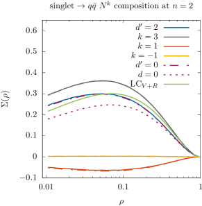
(a)

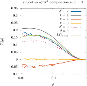
(b)

Figure 6: The jet veto cross section in $V\to q\bar{q}$ for different gluon multiplicities ($n=2,3$). Also shown are the individual contributions at each order of $N_{c}^{k}$ for $d=0$, $d^{\prime}=0$ and $d^{\prime}=2$. See text for details.

Figure 7: The jet veto cross section in (a) $H\to gg$ and (b) $V\to q\bar{q}$ for different gluon multiplicities. Results are shown for $d=0$ and $d=2$. We show the contributions from $n=0$ up to $4$ emissions, however the complete result sums over all emissions (in practice we have limited the simulation to $n\leq 40$ emissions).

Conclusions – This paper represents a major milestone in a project to compute numerically full-colour evolution in perturbative QCD. The inclusion of subleading colour effects will improve the accuracy of future simulation codes and, as a result, be of considerable value to experimenters and theorists interested in performing percent-level simulations for current and future colliders. For the future, we intend to go beyond the soft approximation and include incoming hadrons.

Acknowledgements – The authors want to thank the Erwin Schrödinger Institute Vienna for support while this work has been finalized. JRF thanks the Institute for Particle Physics Phenomenology in Durham for the award of an Associateship. This work has received funding from the UK Science and Technology Facilities Council, the European Union’s Horizon 2020 research and innovation programme as part of the Marie Skłodowska-Curie Innovative Training Network MCnetITN3 (grant agreement no. 722104), and in part by the COST actions CA16201 “PARTICLEFACE” and CA16108 “VBSCAN”. We are grateful to Thomas Becher, Jack Holguin, Mike Seymour, Malin Sjödahl, and René Ángeles Martínez for discussions.

References

- Note (1) CVolver stands for Colour Virtual Evolver, and originates from the studies first presented in Plätzer (2014).
- Bähr et al. (2008) M. Bähr et al., Eur. Phys. J. C58, 639 (2008), arXiv:0803.0883 [hep-ph] .
- Bellm et al. (2016) J. Bellm et al., Eur. Phys. J. C76, 196 (2016), arXiv:1512.01178 [hep-ph] .
- Sjöstrand et al. (2015) T. Sjöstrand et al., Comput. Phys. Commun. 191, 159 (2015), arXiv:1410.3012 [hep-ph] .
- Bothmann et al. (2019) E. Bothmann et al. (Sherpa), SciPost Phys. 7, 034 (2019), arXiv:1905.09127 [hep-ph] .
- Nagy and Soper (2012) Z. Nagy and D. E. Soper, JHEP 06, 044 (2012), arXiv:1202.4496 [hep-ph] .
- Nagy and Soper (2015) Z. Nagy and D. E. Soper, JHEP 07, 119 (2015), arXiv:1501.00778 [hep-ph] .
- Martínez et al. (2018) R. Á. Martínez, M. De Angelis, J. R. Forshaw, S. Plätzer, and M. H. Seymour, (2018), arXiv:1802.08531 [hep-ph] .
- Forshaw et al. (2019) J. R. Forshaw, J. Holguin, and S. Plätzer, JHEP 08, 145 (2019), arXiv:1905.08686 [hep-ph] .
- Nagy and Soper (2019a) Z. Nagy and D. E. Soper, Phys. Rev. D 100, 074012 (2019a), arXiv:1905.07176 [hep-ph] .
- Nagy and Soper (2019b) Z. Nagy and D. E. Soper, Phys. Rev. D 99, 054009 (2019b), arXiv:1902.02105 [hep-ph] .
- Forshaw et al. (2020) J. R. Forshaw, J. Holguin, and S. Plätzer, (2020), arXiv:2003.06400 [hep-ph] .
- Note (2) For processes with two or more coloured particles in both the initial and final state of the hard process, Coulomb/Glauber exchanges are also needed.
- Plätzer (2014) S. Plätzer, Eur. Phys. J. C74, 2907 (2014), arXiv:1312.2448 [hep-ph] .
- Note (3) The improvement is only relevant if there are quarks in the hard process since always vanishes for purely gluonic states.
- Holguin et al. (2020) J. Holguin, J. R. Forshaw, and S. Plätzer, (2020), arXiv:2003.06399 [hep-ph] .
- Platzer and Sjodahl (2012) S. Platzer and M. Sjodahl, Eur. Phys. J. Plus 127, 26 (2012), arXiv:1108.6180 [hep-ph] .
- Kleiss and Verheyen (2016) R. Kleiss and R. Verheyen, Eur.Phys.J.C 76, 359 (2016), arXiv:1605.09246 [hep-ph] .
- Note (4) One notable exception being the numerical summation of the hemisphere jet mass in collisions in Hagiwara et al. (2016).
- Hagiwara et al. (2016) Y. Hagiwara, Y. Hatta, and T. Ueda, Phys. Lett. B 756, 254 (2016), arXiv:1507.07641 [hep-ph] .