Phase-Noise Compensation for OFDM Systems Exploiting Coherence Bandwidth:
Modeling, Algorithms, and Analysis

Abstract

Phase-noise (PN) estimation and compensation are crucial in millimeter-wave (mmWave) communication systems to achieve high reliability. The PN estimation, however, suffers from high computational complexity due to its fundamental characteristics, such as spectral spreading and fast-varying fluctuations. In this paper, we propose a new framework for low-complexity PN compensation in orthogonal frequency-division multiplexing systems. The proposed framework also includes a pilot allocation strategy to minimize its overhead. The key ideas are to exploit the coherence bandwidth of mmWave systems and to approximate the actual PN spectrum with its dominant components, resulting in a non-iterative solution by using linear minimum mean squared-error estimation. The proposed method obtains a reduction of more than $2.5\times$ in total complexity, as compared to the existing methods. Furthermore, we derive closed-form expressions for normalized mean squared-errors (NMSEs) as a function of critical system parameters, which help in understanding the NMSE behavior in low and high signal-to-noise ratio regimes. Lastly, we study a trade-off between performance and pilot-overhead to provide insight into an appropriate approximation of the PN spectrum.

I Introduction

The range of frequencies from $30\text{\,}\mathrm{GHz}$ to $300\text{\,}\mathrm{GHz}$ is usually referred to as the millimeter-wave (mmWave) band. A key feature is that there is an abundant spectrum available to support ultra-high data rate transmission. Owing to this, the mmWave bands have attracted considerable attention [2, 3, 4, 5]. A critical issue, however, is that severe phase-noise (PN) arises from a local oscillator (LO) in practical mmWave systems. The PN increases with the carrier frequency [6], resulting in a 20–40 times higher PN than LOs for sub-$6\text{\,}\mathrm{GHz}$ [7]. The non-negligible amount of PN inevitably leads to significant performance degradation in coherent systems [8]. New modulation techniques, such as orthogonal time frequency modulation (OTFS) [9] and frequency-domain multiplexing with a frequency-domain cyclic prefix (FDM-FDCP) [10], have been recently introduced to tackle this problem in mmWave communications. In orthogonal frequency-division multiplexing (OFDM) systems, the performance drop by PN has been demonstrated using various metrics, such as signal-to-interference-plus-noise ratio (SINR) [11, 12, 13, 14, 15], bit error rate (BER) [11, 16], and channel capacity [17]. To perform coherent detection in mmWave OFDM systems, it is imperative to estimate and compensate the combined effect of PN and the wireless channel, which is a multiplicative process in the time domain, and a circular convolution process in the frequency domain [15]. Unfortunately, this is not a simple task due to the following characteristics of PN in OFDM systems:

• Spectral spreading: PN brings about spectral spreading of the ideal Dirac-delta impulse at the LO’s frequency. The spectral spreading of PN has two detrimental effects on the performance of OFDM systems. One is the common rotation on all subcarriers of an OFDM symbol, called common phase error (CPE); the other is inter-carrier interference (ICI), which destroys orthogonality of subcarriers. As PN increases, it results in higher ICI from neighboring subcarriers.

• Fast-varying fluctuations: The PN process is fast-varying so that there is a low correlation across consecutive OFDM symbols, resulting in estimation and compensation for each OFDM symbol. It requires a stringent latency requirement or high buffer cost for PN estimation.

The problem of simultaneously dealing with both spectral spreading and fast-varying fluctuations is especially challenging in the presence of severe PN. In the OFDM system, the effective channel coefficient is entanglement of two unknown variables of PN and wireless channel components. For this reason, the required estimation problem of effective channel coefficients is formulated as an underdetermined system, which generally has infinitely many solutions. Obtaining an accurate solution is, therefore, not guaranteed. One could argue that, it is possible to solve this problem by using a Bayesian approach [18]. However, it might require high-computational complexity, which makes it more challenging to meet the requirement that the PN estimate must be updated every OFDM symbol.

The problem of severe PN continues to be a significant challenge in multi-antenna systems, i.e, multiple-input multiple-output (MIMO), based on coherent beamforming. Recently, [19, 20, 21, 22, 23] have investigated the impact of such PN at large-scale antenna systems, so-called massive MIMO. [19, 20] have analytically shown the PN impact on the performance of precoders /equalizers at massive MIMO base station (BS). It has been generalized with hardware impairments including multiplicative phase-drifts and additive distortion noise [21, 22, 23]. A common observation in the previous research is that, increasing the number of antennas can be beneficial for PN mitigation since the phase-drifts average out. However, separate LOs for each antenna are required to obtain such benefits, resulting in high-cost hardware architecture.

Plenty of methods for PN estimation and compensation have been investigated in [24, 25, 26, 27, 28, 29, 30, 31, 32, 33, 34]. Early studies on PN compensation have used quite strong assumptions such as small PN [24, 25] and perfect channel state information [26, 27] at the receiver. In the case where both PN and channel state information are unknown, joint channel and PN estimation [28, 29], iterative joint PN estimation and data detection [30, 31] have been presented. However, such techniques may be too complicated to be implemented in practical wireless systems.

Pilot-assisted transmission simplifies the challenging task of receiver design for coherent processing in general. The use of pilots may also be beneficial to achieve low-complexity estimation or to acquire the instantaneous channel coefficients. In this regard, a dedicated pilot symbol for phase tracking, called Phase Tracking Reference Signal (PTRS), has been introduced in the 3rd Generation Partnership Project (3GPP) New Radio (NR) [35]. Motivated by this fact, [32, 33, 34] have designed the dedicated pilot pattern for PN tracking so that it has a high density in the time domain to tackle the low correlation of PN across OFDM symbols. These solutions, however, have been focused on tracking only CPE while there is no consideration to estimate the performance limiting ICI components in mmWave systems.

Contributions: We develop a novel framework for low-complexity PN compensation for OFDM systems. The key ideas are to exploit the coherence bandwidth of mmWave systems and to approximate the actual PN spectrum with its dominant components. Our main contributions are summarized as follows:

• We reformulate the joint estimation problem of PN and channel from an underdetermined system into a system with the same number of observations and unknowns, which enables low-complexity PN estimation by using least-squares (LS) and linear minimum mean squared-error (LMMSE) estimators. The proposed algorithm obtains a reduction of more than $2.5\times$ in total complexity, as compared to the existing method.

• We design a pilot pattern that has a carefully selected set of symbols to estimate the combined effect of dominant PN components and channel frequency response. Furthermore, the minimum pilot-overhead ratio for our proposed method is quantified with a set of system parameters related to the channel coherence structure.

• We derive closed-form expressions for normalized mean squared-errors of each estimator for joint PN and channel estimation. These expressions are represented as a function of OFDM parameters, LO quality, signal-to-noise ratio (SNR), and approximation order of the PN spectrum. Further, this helps in understanding the NMSE behavior in low and high SNR regimes, providing an informative guideline for pilot allocation in mmWave OFDM systems.

• We present a trade-off between performance and pilot-overhead. For the analysis, the BER and throughput performance of the proposed method are evaluated. This trade-off provides insight into an appropriate approximation of the PN spectrum, according to SNR and PN environments.

Notation: The set of complex numbers is denoted by $\mathbb{C}$. Lowercase boldface letters stand for column vectors and uppercase boldface letters designate matrices. For a vector or a matrix, we denote its transpose, conjugate, and conjugate transpose $\mathbf{(\cdot)}^{\rm T}$, $\mathbf{(\cdot)}^{*}$, and $\mathbf{(\cdot)}^{\rm H}$, respectively; the subscript notations $\mathbf{(\cdot)}_{\rm t}$ and $\mathbf{(\cdot)}_{\rm f}$ stand for the time- and frequency-domain representations of a vector or a matrix. The $N\times N$ identity matrix is denoted by $\mathbf{I}_{N}$, and the $N\times M$ all-zeros matrix by $\mathbf{0}_{N\times M}$. The expectation operator and Euclidean norm is denoted by ${\mathbb{E}}[\mathbf{\cdot}]$ and $\|\mathbf{\cdot}\|_{2}$, respectively. Sets are designated by upper-case calligraphic letters; the cardinality and complement of the set $\mathcal{T}$ is $|\mathcal{T}|$ and $\mathcal{T}^{c}$, respectively; the difference between two sets $\mathcal{T}$ and $\mathcal{F}$ is denoted by $\mathcal{T}\setminus\mathcal{F}$. The operators for circular convolution, deconvolution, and Hadamard product are written as $\circledast$, $\circledast^{-1}$, and $\circ$, respectively; $\lfloor x\rfloor$ and $\lceil x\rceil$ denote the greatest/least integer less/greater than or equal to $x$.

Outline: The remainder of this paper is organized as follows: In Section II, we describe the system model under consideration. Section III describes the proposed PN and channel compensation algorithm. In Section IV, we analyze the NMSE performance of the proposed method by numerical evaluation. Section V addresses the pilot-overhead and the computational complexity of our proposed algorithm. Section VI present the trade-off between performance and pilot-overhead. A summary and concluding remarks appear in Section VII.

II System Description and Preliminaries

In this section, we briefly overview our basic idea to tackle the joint estimation problem of PN and channel frequency response and compare it with the approach of existing solutions. Before moving on to this, we first present the system and PN models that will be used in this paper.

II-A System Model

We consider an OFDM system with $N$ subcarriers, a sampling period $T_{\rm s}$, a subcarrier spacing $\Delta f$, and a bandwidth $B=1/T_{\rm s}=N\Delta f$. Let $\{X_{k}\}_{k=0}^{N-1}$ be the transmitted symbol sequence across $N$ subcarriers of an OFDM symbol, with an average per-symbol power constraint $\mathbb{E}[|X_{k}|^{2}]=E_{\rm s}$. An $N$-point unitary inverse discrete Fourier transform (IDFT) of $\{X_{k}\}_{k=0}^{N-1}$ provides the time-domain representation of the OFDM symbol as

$$x_{n}={\frac{1}{\sqrt{N}}}{\sum_{k=0}^{N-1}}X_{k}e^{j2\pi kn/N},$$ (1)

where time index $n\in\{-N_{\rm cp},-N_{\rm cp}+1,\cdots,0,1,\ldots,N-1\}$. Each OFDM symbol is assumed to consist of a cyclic prefix (CP) of length-$N_{\rm cp}$ samples.

For our subsequent analysis, we adopt the coherence block model with a coherence time $T_{\rm c}$ and a coherence bandwidth $B_{\rm c}$. In this model, there are two parameters widely used in the literature [36, 37, 38]. One is the number of OFDM symbols within $T_{\rm c}$, and the other is the number of subcarriers within $B_{\rm c}$. These parameters are defined as

$$N_{\rm ct}\triangleq\lfloor{T_{\rm c}}/{T_{\rm sym}}\rfloor,$$ (2)

$$N_{\rm cb}\triangleq\lfloor{B_{\rm c}}/{\Delta f}\rfloor,$$ (3)

where $T_{\rm sym}$ the duration of one OFDM symbol. We assume that the coherence block spans $N_{\rm ct}$ and $N_{\rm cb}$ successive OFDM symbols and subcarriers, over which the channel impulse and frequency response, respectively, is constant.

II-B Phase Noise Model

We consider the model introduced in [39] to illustrate the PN of a free-running oscillator. The PN is defined as

$$\phi(t)=2\pi f_{\rm o}\eta(t)$$ (4)

where $f_{\rm o}$ denotes an oscillator frequency. A random time shift $\eta(t)$ becomes, asymptotically with time, a Wiener process as

$$\eta(t)=\sqrt{c}W(t),$$ (5)

where $c$ denotes the parameter indicating an oscillator quality; $W(t)$ represents a Wiener process having an accumulated Gaussian random variable with i.i.d. $\mathcal{N}(0,1)$, i.e., $W(t_{2})-W(t_{1})\propto\hskip 1.25pt\mathcal{N}(0,\sqrt{\Delta t})$ where $\Delta t=\mid t_{2}-t_{1}\mid$. The variance of the Wiener process $\eta(t)$ increases linearly with the time difference $\Delta t$, i.e., $\sigma_{\eta}^{2}=c\Delta t$. According to (4), $\phi(t)$ is also a Wiener process with zero mean and variance $2\pi\beta\Delta t$, where $\beta$ denotes the two-sided 3-$\mathrm{dB}$ linewidth of the Lorentzian power spectral density [11].

II-C OFDM Signal Model with Phase Noise

The PN at the receiver influences the channel output as an angular multiplicative distortion in the time domain. Then, the received signal in the time domain ${\mathbf{y}_{\rm{t}}}\in\mathbb{C}^{N\times 1}$ is

$$\begin{split}{\mathbf{y}_{\rm{t}}}&=\mathbf{p}_{\rm t}\circ({\mathbf{x}_{\rm{t}}}\circledast{\mathbf{h}_{\rm{t}}})+{\mathbf{z}_{\rm{t}}}\\ &={\mathbf{\Phi}}_{\rm t}({\mathbf{x}}_{\rm t}\circledast{\mathbf{h}}_{\rm t})+{\mathbf{z}}_{\rm t},\end{split}$$ (6)

where $\mathbf{p}_{\rm t}=[e^{j\phi_{0}},e^{j\phi_{1}},\cdots,e^{j\phi_{N-1}}]^{\rm T}\in\mathbb{C}^{N\times 1}$ is the PN realization during one OFDM symbol, $\mathbf{x}_{\rm{t}}\in\mathbb{C}^{N\times 1}$ the transmitted signal, $\mathbf{h}_{\rm{t}}\in\mathbb{C}^{N\times 1}$ the channel impulse response, ${\mathbf{z}_{\rm{t}}}\in\mathbb{C}^{N\times 1}$ the additive white Gaussian noise (AWGN) with i.i.d. ${\mathcal{CN}}\left(0,\sigma_{z}^{2}\right)$ entries, and $\mathbf{\Phi}_{\rm{t}}={\rm{diag}}\{e^{j\phi_{n}}\}_{n=0}^{N-1}\in\mathbb{C}^{N\times N}$ the diagonal matrix with the entries of $\mathbf{p}_{\rm t}$ on its main diagonal. In view of the duality, the discrete Fourier transform (DFT) of a product of two finite-length sequences is the circular convolution of their respective DFTs [40]. Thus, the received signal in the frequency domain ${\mathbf{y}_{\rm{f}}}\in\mathbb{C}^{N\times 1}$ is

$$\begin{split}{\mathbf{y}_{\rm{f}}}&={\mathbf{p}_{\rm{f}}}\circledast({\mathbf{x}_{\rm{f}}}\circ{\mathbf{h}_{\rm{f}}})+{\mathbf{z}_{\rm{f}}}\\ &=\mathbf{\Phi}_{\rm{f}}{\mathbf{H}_{\rm f}}{\mathbf{x}_{\rm{f}}}+{\mathbf{z}_{\rm{f}}},\end{split}$$ (7)

where $\mathbf{p}_{\rm{f}}=[P_{0},P_{1},\cdots,P_{N-1}]^{\rm T}\in\mathbb{C}^{N\times 1}$ is the DFT coefficient vector of the time-domain PN sequence $\{e^{j\phi_{n}}\}_{n=0}^{N-1}$, i.e., $P_{i}=\frac{1}{N}\sum_{n=0}^{N-1}e^{j\phi_{n}}e^{-j2\pi ni/N}$; $\mathbf{x}_{\rm{f}}=[X_{0},X_{1},\cdots,X_{N-1}]^{\rm T}$, $\mathbf{h}_{\rm{f}}=[H_{0},H_{1},\cdots,H_{N-1}]^{\rm T}$, $\mathbf{z}_{\rm{f}}=[Z_{0},Z_{1},\cdots,Z_{N-1}]^{\rm T}\in\mathbb{C}^{N\times 1}$ the transmit symbol, channel frequency fresponse, and noise, respectively, in the frequency domain; $\mathbf{\Phi}_{\rm{f}}={{\rm circ}(\mathbf{p}_{\rm f})}$ is a circulant matrix formed by the spectral PN components,

$$\mathbf{\Phi}_{\rm{f}}=\begin{bmatrix}P_{0}&P_{N-1}&P_{N-2}&\cdots&\cdots&P_{1}\\ P_{1}&P_{0}&P_{N-1}&\cdots&\cdots&P_{2}\\ P_{2}&P_{1}&P_{0}&P_{N-1}&\ddots&P_{3}\\ \vdots&\ddots&\ddots&\ddots&\ddots&\vdots\\ P_{N-2}&P_{N-3}&\cdots&P_{1}&P_{0}&P_{N-1}\\ P_{N-1}&P_{N-2}&\cdots&P_{2}&P_{1}&P_{0}\end{bmatrix},$$ (8)

${\mathbf{H}_{\rm f}}={\rm diag}\{H_{k}\}_{k=0}^{N-1}$ is the diagonal matrix with the entries of $\mathbf{h}_{\rm f}$ on its main diagonal. Given the coherence block model, we denote the number of coherence blocks $N_{\rm c}$. Thus, the channel frequency response consists of $N_{\rm c}$ different channel coefficients, with i.i.d. $\mathcal{CN}(0,1)$ entries, and its index set is denoted $\mathcal{C}$, i.e., $\{H_{k}\}_{k=0}^{N_{\rm c}-1},k\in\mathcal{C}$. To look into the CPE and the ICI effect on the received signal for each subcarrier $k\in\{0,1,\cdots,N-1\}$, let us rewrite (7) in the sample-wise form

$$Y_{k}=\underbrace{P_{0}}_{\rm CPE}H_{k}X_{k}+\underbrace{{\sum_{\ell=0,\ell\neq k}^{N-1}}P_{(k-\ell)_{N}}H_{\ell}X_{\ell}}_{\rm ICI}+Z_{k},$$ (9)

where $(\cdot)_{N}$ denotes the modulo-$N$ operation. In the absence of PN, by the fact that $P_{i}$ is a Kronecker delta function $\delta[i]$, the received signal (9) becomes

$$Y_{k}=X_{k}H_{k}+Z_{k}.$$ (10)

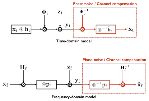
Figure 1: Basic model of PN/channel compensation and detection in time and frequency domains.

II-D Phase Noise and Channel Compensation Model

In this subsection, we provide a brief comparison of the conventional and proposed approaches for PN and channel compensation. Fig. 1 displays the basic model of PN/channel compensation and detection, where $\hat{(\cdot)}$ designates the corresponding estimated or decoded vector/matrix. Researchers have investigated how to efficiently reduce the unknowns to handle the underdetermined problem of joint PN and channel estimation, which led to low-complexity estimation methods. A popular approach is to utilize the fact that the channel impulse response $\mathbf{h}_{\rm t}$ in the time domain has fewer parameters than in the frequency response, resulting in time-domain channel estimation with a smaller number of unknowns. Based on this fact, the joint estimation algorithms for frequency-domain PN [41, 42], and time-domain PN [43, 44], respectively, have been presented. The basic technique used in [41, 42, 43, 44] is a joint least-squares estimation. Especially, [42] introduced a new constraint by the geometrical property of spectral PN components to complement the weakness of the relaxed constraint used in [41]. Further, [44] showed to be able to reduce the computational complexity of least-squares estimation significantly by using the majorization-minimization technique. However, the above least-squares estimation methods require a full-pilot OFDM symbol to perform joint PN and channel estimation, translating into significant pilot overhead.

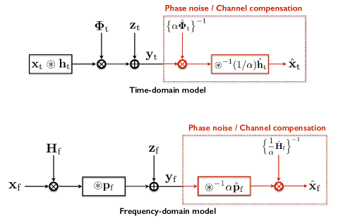
Figure 2: Proposed model of PN/channel compensation and detection in time and frequency domains.

In contrast to the existing approach, we consider channel coherence in the frequency domain to manage the underdetermined problem. The coherence bandwidth of a mmWave system is inherently much larger than those of conventional systems [45]. It is a promising basis for more suitable PN compensation in mmWave systems. Larger coherence bandwidth can facilitate the estimation of scaled PN components in the frequency domain, i.e., $\alpha\hat{\mathbf{p}}_{\rm f}$, $\alpha\in\mathbb{C}$, as illustrated in Fig. 2. The deconvolution by the scaled PN estimates suppresses the effect of ICI by PN, translating it into a simple estimation problem for $(1/\alpha)\mathbf{h}_{\rm f}$, which can be estimated by using as many pilots as there are channel coefficients in $\mathbf{h}_{\rm f}$.

II-E Effective Channel with Large Coherence Bandwidth

The effective channel coefficient can be recovered, provided that there are as many observations as unknowns. To see how coherence bandwidth could be utilized to meet this condition, let us go through two examples. Let $N_{\rm p}$ denote the number of dominant PN components in the frequency domain.

Example 1: Consider four received samples as shown in (9) when $N_{\rm cb}=1$ and $N_{\rm p}=3$.

$$\begin{split}Y_{0}&=\underbrace{P_{0}}_{\rm CPE}H_{0}X_{0}+\underbrace{P_{1}H_{N-1}X_{N-1}+P_{N-1}H_{1}X_{1}}_{\rm dominant\ ICI}\\ &\;\;\;+{\sum_{{\ell}\in\mathcal{L}\setminus\{0,1,N-1\}}}P_{(0-\ell)_{N}}H_{\ell}X_{\ell}+Z_{0},\\ Y_{1}&=\underbrace{P_{0}}_{\rm CPE}H_{1}X_{1}+\underbrace{P_{1}H_{0}X_{0}+P_{N-1}H_{2}X_{2}}_{\rm dominant\ ICI}\\ &\;\;\;+{\sum_{{\ell}\in\mathcal{L}\setminus\{0,1,2\}}}P_{(1-\ell)_{N}}H_{\ell}X_{\ell}+Z_{1},\\ Y_{2}&=\underbrace{P_{0}}_{\rm CPE}H_{2}X_{2}+\underbrace{P_{1}H_{1}X_{1}+P_{N-1}H_{3}X_{3}}_{\rm dominant\ ICI}\\ &\;\;\;+{\sum_{{\ell}\in\mathcal{L}\setminus\{1,2,3\}}}P_{(2-\ell)_{N}}H_{\ell}X_{\ell}+Z_{2},\\ Y_{3}&=\underbrace{P_{0}}_{\rm CPE}H_{3}X_{3}+\underbrace{P_{1}H_{2}X_{2}+P_{N-1}H_{4}X_{4}}_{\rm dominant\ ICI}\\ &\;\;\;+{\sum_{{\ell}\in\mathcal{L}\setminus\{2,3,4\}}}P_{(3-\ell)_{N}}H_{\ell}X_{\ell}+Z_{3},\\ \end{split}$$ (11)

where subcarrier index $\ell\in\mathcal{L}\triangleq\{0,1,...,N-1\}$. Assume that ICI terms represented by the summation operator and noise components are negligible, and all transmitted symbols are used as pilots. In the four observations, there are twelve different unknowns, i.e., $\{P_{0}H_{k}\}_{k=0}^{3}$, $\{P_{1}H_{k}\}_{k=N-1,0}^{2}$, and $\{P_{N-1}H_{k}\}_{k=1}^{4}$, being underdetermined.

Example 2: Consider the same number of received samples when $N_{\rm cb}=6$ and $N_{\rm p}=3$ as follows.

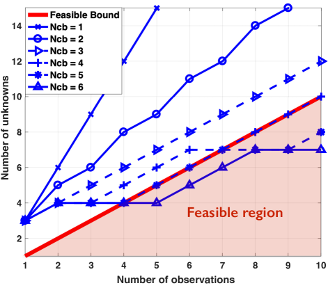
Figure 3: The total number of effective channel unknowns involved in the corresponding numbers of observations according to $N_{\rm cb}$ ($N_{\rm p}=3$).

$$\begin{split}Y_{0}&=\underbrace{P_{0}}_{\rm CPE}H_{0}X_{0}+\underbrace{P_{1}H_{\lceil{(N-1)/6}\rceil}X_{N-1}+P_{N-1}H_{0}X_{1}}_{\rm dominant\ ICI}\\ &\;\;\;+{\sum_{{\ell}\in\mathcal{L}\setminus\{0,1,N-1\}}}P_{(0-\ell)_{N}}H_{\lfloor{\ell/6}\rfloor}X_{\ell}+Z_{0},\\ Y_{1}&=\underbrace{P_{0}}_{\rm CPE}H_{0}X_{1}+\underbrace{P_{1}H_{0}X_{0}+P_{N-1}H_{0}X_{2}}_{\rm dominant\ ICI}\\ &\;\;\;+{\sum_{{\ell}\in\mathcal{L}\setminus\{0,1,2\}}}P_{(1-\ell)_{N}}H_{\lfloor{\ell/6}\rfloor}X_{\ell}+Z_{1},\\ Y_{2}&=\underbrace{P_{0}}_{\rm CPE}H_{0}X_{2}+\underbrace{P_{1}H_{0}X_{1}+P_{N-1}H_{0}X_{3}}_{\rm dominant\ ICI}\\ &\;\;\;+{\sum_{{\ell}\in\mathcal{L}\setminus\{1,2,3\}}}P_{(2-\ell)_{N}}H_{\lfloor{\ell/6}\rfloor}X_{\ell}+Z_{2},\\ Y_{3}&=\underbrace{P_{0}}_{\rm CPE}H_{0}X_{3}+\underbrace{P_{1}H_{0}X_{2}+P_{N-1}H_{0}X_{4}}_{\rm dominant\ ICI}\\ &\;\;\;+{\sum_{{\ell}\in\mathcal{L}\setminus\{2,3,4\}}}P_{(3-\ell)_{N}}H_{\lfloor{\ell/6}\rfloor}X_{\ell}+Z_{3}.\\ \end{split}$$ (12)

In this case, it is possible to recover all effective channel coefficients because there are only as many unknowns as observations. Fig. 3 shows the total number of effective channel unknowns involved in the corresponding numbers of observations, according to $N_{\rm cb}$, when $N_{\rm p}=3$. For channel frequency responses with $N_{\rm cb}$ larger than three, there are fewer unknowns than observations. With this insight, in the next section, we describe a low-complexity PN/channel estimation followed by the NMSE analysis.

III Proposed Algorithm

Exploiting the approximation of the PN spectrum and large coherence bandwidth, the joint estimation problem of PN and channel can be reformulated from a heavily underdetermined system into a system with the same number of equations and unknowns, referred to as a fully determined linear system. This enables low-complexity PN/channel estimation by using the LS and LMMSE estimators. In the proposed algorithm, two kinds of frequency-domain estimations are required. One is for the $N_{\rm p}$ dominant PN components scaled by $\alpha$ and the other for the $N_{\rm c}$ scaled-channel coefficients, as illustrated in Fig. 2.

To define dominant PN components, we adopt $\gamma$ as the approximation order of the PN spectrum, where $N_{\rm p}=2\gamma+1$ for $\gamma\in\{0,1,\cdots,N/2\}$. The index set of dominant PN is defined as $\mathcal{P}\triangleq\{0,1,\cdots,N-1\}\setminus\{\gamma+1,\gamma+2,\cdots,N-(\gamma+1)\}$. Let $\mathbf{p}_{\rm{f},\gamma}\in\mathbb{C}^{N\times 1}$ be the approximated PN vector where $P_{i}=0$, $i\in\mathcal{P}^{\rm c}$, and $\mathbf{e}_{\rm f,app}\triangleq\mathbf{p}_{\rm f}-\mathbf{p}_{{\rm f},\gamma}\in\mathbb{C}^{N\times 1}$ be the approximation error vector, e.g., $\mathbf{p}_{\rm{f},2}=[P_{0},P_{1},P_{2},0,\cdots,0,P_{N-2},P_{N-1}]^{\rm T}$ and $\mathbf{e}_{\rm f,app}=[\mathbf{0}_{1\times 3},P_{3},P_{4},\cdots,P_{N-(\gamma+1)},\mathbf{0}_{1\times 2}]^{\rm T}$ for $\gamma=2$. The frequency-domain effective channel component in (7) is defined as $F_{i,k}\triangleq P_{i}H_{k}$, which is the element in a set of multiplications between $P_{i}$ and $H_{k}$ for $i\in\mathcal{P}$ and $k\in\mathcal{C}$. We call this PN-affected channel. With the $\gamma$-order approximation, the PN-affected-channel matrix ${\mathbf{F}}_{\gamma}$ and the approximation error matrix ${\mathbf{E}}_{\gamma}$ are, respectively,

$${\mathbf{F}}_{\gamma}=\mathbf{\Phi}_{\rm{f},\gamma}{\mathbf{H}_{\rm f}},\text{and}$$ (13)

$${\mathbf{E}}_{\gamma}=\mathbf{F}-{\mathbf{F}}_{\gamma}=\tilde{\mathbf{\Phi}}_{\rm f,\gamma}\mathbf{H}_{\rm f},$$ (14)

where $\mathbf{\Phi}_{\rm{f},\gamma}={{\rm circ}(\mathbf{p}_{\rm{f},\gamma})}$, $\tilde{\mathbf{\Phi}}_{\rm f,\gamma}={{\rm circ}(\mathbf{e}_{\rm f,app})}$, and ${\mathbf{F}}=\mathbf{\Phi}_{\rm{f}}{\mathbf{H}_{\rm f}}$. One of the columns in $\mathbf{F}_{\gamma}$ is estimated for ICI suppression, which includes $N_{\rm p}$ dominant PN components scaled by $\alpha$. As a result of the ICI suppression, the Toeplitz convolution matrix (13) is converted into a diagonal matrix of which diagonal elements are called the ICI-free channel in this paper. Fig. 4 illustrates the proposed architecture with PN-affected- and ICI-free-channel estimation. Before explaining the details of proposed algorithm, we first describe the transmission structure in the following subsection.

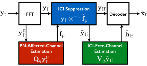
Figure 4: System overview of the proposed PN/channel compensation architecture. For the PN-affected-estimator $\mathbf{Q}_{q}$ and ICI-free-channel estimator $\mathbf{V}_{q}$, the LS and LMMSE estimators are applied, i.e., $q\in\{\mathsf{ls},\mathsf{lmmse}\}$.

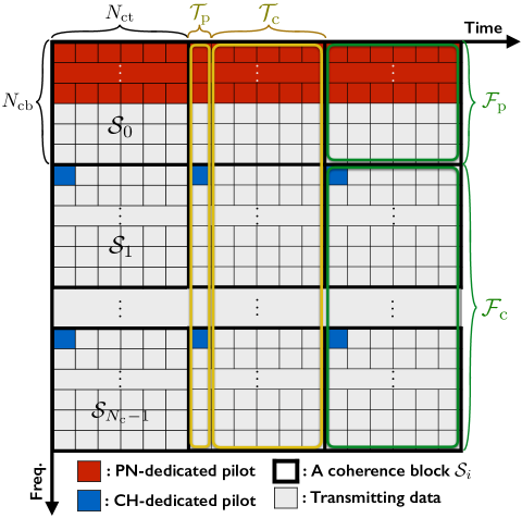
Figure 5: An example of transmission structure for PN-affected- and ICI-free-channel estimation. Based on a set of coherence blocks across $N$ subcarriers, $\mathcal{S}=\mathcal{S}_{0}\cup\mathcal{S}_{1}\cup\cdots\mathcal{S}_{N_{\rm c}-1}$, the pattern for resource allocation is identical.

III-A Transmission Structure

Let us define a coherence block $\mathcal{S}_{k}$, $k\in\mathcal{C}$ with cardinality $|\mathcal{S}_{k}|=N_{\rm cb}N_{\rm ct}$, and $\mathcal{S}=\mathcal{S}_{0}\cup\mathcal{S}_{1}\cup\cdots\mathcal{S}_{N_{\rm c}-1}$ be a set of non-overlapping coherence blocks across $N$ subcarriers, i.e., $|\mathcal{S}|=N_{\rm c}N_{\rm cb}N_{\rm ct}$, as illustrated in Fig. 5. To describe resource allocation for pilots and transmitting data, we divide $\mathcal{S}$ into two subsets in the frequency and time domain, respectively; $\mathcal{F}_{\rm p}$ and $\mathcal{F}_{\rm c}$ in the frequency domain, and $\mathcal{T}_{\rm p}$ and $\mathcal{T}_{\rm c}$ in the time domain, where $\mathcal{S}=\mathcal{F}_{\rm p}\cup\mathcal{F}_{\rm c}=\mathcal{T}_{\rm p}\cup\mathcal{T}_{\rm c}$ and $\mathcal{F}_{\rm p}\cap\mathcal{F}_{\rm c}=\mathcal{T}_{\rm p}\cap\mathcal{T}_{\rm c}=\phi$. In the frequency domain, $\mathcal{F}_{\rm p}$ designate the coherence block set that includes PN-dedicated pilot for PN-affected-channel estimation, and $\mathcal{F}_{\rm c}$ involves CH-dedicated pilot for ICI-free-channel estimation. An example of transmission structure for PN-affected- and ICI-free-channel estimation is shown in Fig. 5. In the time domain, we consider the fact that the PN process is fast-varying within channel coherence time while the wireless channel is invariant, resulting in the PN-affected-channel estimation of each OFDM symbol. Hence, only the PN-dedicated pilot is allocated in $\mathcal{T}_{\rm c}$ while both pilots in $\mathcal{T}_{\rm p}$. The remainder of the coherence block is used for transmitting data.

III-B PN-Affected-Channel Estimation

In this subsection, we elaborate on the PN-affected-channel estimation with the following example.

Example 3 (PN-Affected-Channel Estimation): Suppose $N_{\rm cb}=6$ and $N_{\rm p}=3$ in this example. Based on (7), (13), and (14), the received signal is

$${\mathbf{y}}_{\rm{f}}={\mathbf{F}}_{1}{\mathbf{x}_{\rm{f}}}+\underbrace{\mathbf{E}_{1}{\mathbf{x}_{\rm{f}}}+{\mathbf{z}_{\rm{f}}}}_{{\mathbf{w}}_{1}}={\mathbf{F}}_{1}{\mathbf{x}_{\rm{f}}}+{\mathbf{w}}_{1},$$ (15)

where $\mathbf{F}_{1}$ is presented in (16) at the top of next page and denotes the 1-order approximated channel matrix; $\mathbf{E}_{1}$ is its approximation error matrix; ${\mathbf{w}}_{1}$ is the ICI by the approximation error plus AWGN.

$${\mathbf{F}}_{1}=\begin{bmatrix}F_{0,0}&F_{N-1,0}&0&\cdots&0&F_{1,N_{\rm c}-1}\\ F_{1,0}&F_{0,0}&F_{N-1,0}&\ddots&\ddots&0\\ 0&F_{1,0}&F_{0,0}&F_{N-1,0}&\ddots&\vdots\\ \vdots&\ddots&\ddots&\ddots&\ddots&0\\ 0&\ddots&\ddots&F_{1,N_{\rm c}-1}&F_{0,N_{\rm c}-1}&F_{N-1,N_{\rm c}-1}\\ F_{N-1,0}&0&\cdots&0&F_{1,N_{\rm c}-1}&F_{0,N_{\rm c}-1}\end{bmatrix}\in\mathbb{C}^{N\times N}.$$ (16)

We denote the PN-affected-channel vector by $\mathbf{f}_{\bar{\rm p}}\in\mathbb{C}^{N_{\rm p}\times 1}$, which consists of dominant PN components scaled by a channel coefficient as

$$\begin{split}{\mathbf{f}}_{\bar{\rm p}}&=[F_{N-\gamma,k},F_{N-\gamma+1,k},\cdots,F_{0,k},\cdots,F_{\gamma-1,k},F_{\gamma,k}]^{\rm T}\\ &=H_{k}\underbrace{[P_{N-\gamma},P_{N-\gamma+1},\cdots,P_{0},\cdots,P_{\gamma-1},P_{\gamma}]^{\rm T}}_{\bar{\mathbf{p}}_{\rm f,\gamma}},\end{split}$$ (17)

where $\bar{\mathbf{p}}_{\rm f,\gamma}\in\mathbb{C}^{N_{\rm p}\times 1}$ is the dominant PN vector with the $\gamma$-order approximation. Based on (17), the coefficient $\alpha$ in Fig. 2 indicates the channel coefficient $H_{k}$ in $\mathcal{S}_{k}$. In this example, $\mathbf{f}_{\bar{\rm p}}=[F_{N-1,k},F_{0,k},F_{1,k}]^{\rm T}\in\mathbb{C}^{3\times 1}$. With the three unknowns in $\mathbf{f}_{\bar{\rm p}}$, a fully determined linear system can be constructed as follows:

$$\begin{split}{\mathbf{y}_{\rm f}^{\rm p}}&={\mathbf{F}_{1}^{\rm p}}{\mathbf{x}_{\rm{f,1}}^{\rm p}}+{\mathbf{w}}_{1}^{\rm p}\\ &=\underbrace{\begin{bmatrix}F_{1,0}&F_{0,0}&F_{N-1,0}&0&0\\ 0&F_{1,0}&F_{0,0}&F_{N-1,0}&0\\ 0&0&F_{1,0}&F_{0,0}&F_{N-1,0}\end{bmatrix}}_{\mathbf{F}_{1}^{\rm p}}\underbrace{\begin{bmatrix}X_{0}^{\rm p}\\ X_{1}^{\rm p}\\ X_{2}^{\rm p}\\ X_{3}^{\rm p}\\ X_{4}^{\rm p}\end{bmatrix}}_{\mathbf{x}_{\rm f,1}^{\rm p}}+{\mathbf{w}}_{1}^{\rm p},\\ \end{split}$$ (18)

where $\mathbf{y}_{\rm f}^{\rm p}=[Y_{1},Y_{2},Y_{3}]^{\rm T}$ is the three observations in $\mathbf{y}_{\rm f}$, and $\mathbf{w}_{1}^{\rm p}\in\mathbb{C}^{3\times 1}$ the corresponding vector in $\mathbf{w}_{1}$; the element in $\mathbf{x}_{\rm f,1}^{\rm p}$ is denoted by $X_{k}^{\rm p}$ to distinguish the PN-dedicated pilot from transmitting data. Using the commutative property, (18) can be rewritten as

$${\mathbf{y}_{\rm f}^{\rm p}}=\underbrace{\begin{bmatrix}X_{2}^{\rm p}&X_{1}^{\rm p}&X_{0}^{\rm p}\\ X_{3}^{\rm p}&X_{2}^{\rm p}&X_{1}^{\rm p}\\ X_{4}^{\rm p}&X_{3}^{\rm p}&X_{2}^{\rm p}\end{bmatrix}}_{\mathbf{X}_{\rm{f,1}}^{\rm p}}\underbrace{\begin{bmatrix}F_{N-1,0}\\ F_{0,0}\\ F_{1,0}\end{bmatrix}}_{\mathbf{f}_{\bar{\rm{p}}}}+{\mathbf{w}}_{1}^{\rm p}.$$ (19)

By the PN-dedicated pilot $\{X_{k}^{\rm p}\}_{k=0}^{4}$ such that ${\rm rank}(\mathbf{X}_{\rm f,1}^{\rm p})=3$, all the unknowns in $\mathbf{f}_{\bar{\rm p}}$ can be estimated. Based on (19), the optimization problem for the optimal PN-dedicated pilot matrix, with respect to the approximation order of $\gamma$, is

$$\underset{\mathbf{X}_{{\rm f},\gamma}^{\rm p}}{\text{minimize}}\quad\|\mathbf{w}_{\gamma}^{\rm p}\|_{\rm F}^{2}$$ (20)

$$\text{subject to}\hskip 10.00002pt{\rm rank}(\mathbf{X}_{{\rm f},\gamma}^{\rm p})=2\gamma+1.$$

The following theorem provides the optimal solution of (20).

Theorem 1.

Assume that the PN-dedicated pilot is allocated in the $\mathcal{S}_{0}$. If a $\gamma$-order approximation of PN spectrum is applied, the optimal PN-dedicated pilot matrix $\mathbf{X}_{{\rm f},\gamma}^{\rm p}\in\mathbb{C}^{N_{\rm p}\times N_{\rm p}}$, for minimizing the ICI by the approximation error, is

$$\mathbf{X}_{{\rm f},\gamma}^{\rm p}=\mathbf{I}_{N_{\rm p}}$$ (21)

where

$$\mathbf{X}_{{\rm f},\gamma}^{\rm p}=\begin{bmatrix}X_{2\gamma}^{\rm p}&X_{2\gamma-1}^{\rm p}&\cdots&\cdots&X_{0}^{\rm p}\\ X_{2\gamma+1}^{\rm p}&X_{2\gamma}^{\rm p}&X_{2\gamma-1}^{\rm p}&\cdots&X_{1}^{\rm p}\\ X_{2\gamma+2}^{\rm p}&X_{2\gamma+1}^{\rm p}&X_{2\gamma}^{\rm p}&\ddots&\vdots\\ \vdots&\ddots&\ddots&\ddots&X_{2\gamma-1}^{\rm p}\\ X_{2\gamma+2\gamma}^{\rm p}&\cdots&X_{2\gamma+2}^{\rm p}&X_{2\gamma+1}^{\rm p}&X_{2\gamma}^{\rm p}\end{bmatrix}$$ (22)

Proof.

See Appendix A ∎

We consider the LS and LMMSE estimators for the PN-affected channel. The optimal PN-dedicated pilot matrix (21) leads to lower computational complexity as compared to the conventional LS and LMMSE estimators [46]. The LS and LMMSE PN-affected-channel estimators, respectively, is (see Appendix B for $\mathbf{Q}_{\mathsf{lmmse}}$)

$$\begin{split}{\mathbf{Q}}_{\mathsf{ls}}&=({\mathbf{X}_{\rm{f,\gamma}}^{\rm p}})^{-1}=\mathbf{I}_{N_{\rm p}},\end{split}$$ (23)

$$\begin{split}{\mathbf{Q}}_{\mathsf{lmmse}}&=\mathbf{R}_{\mathbf{p}\mathbf{p}}^{\gamma}\{\mathbf{R}_{\mathbf{p}\mathbf{p}}^{\gamma}+\mathbf{R}_{\mathbf{ici}}^{\gamma}+\frac{1}{\mathsf{SNR}}{\mathbf{I}_{N_{\rm p}}}\}^{-1},\end{split}$$ (24)

where $\mathbf{R}_{\mathbf{p}\mathbf{p}}^{\gamma}=\mathbb{E}\{\bar{\mathbf{p}}_{{\rm f},\gamma}(\bar{\mathbf{p}}_{{\rm f},\gamma})^{\rm H}\}$ is the autocorrelation matrix of $\bar{\mathbf{p}}_{{\rm f},\gamma}$ in (17) and $\mathbf{R}_{\mathbf{ici}}^{\gamma}$ the autocorrelation matrix of ICI vector arising from the $\gamma$-order-approximation error; ${\mathsf{SNR}}\triangleq E_{\rm s}/\sigma_{z}^{2}$ the average SNR. The LS/LMMSE estimate of $\mathbf{f}_{\bar{\rm p}}$ is

$$\begin{split}{\hat{\mathbf{f}}}_{\bar{\rm p},q}&={{\mathbf{Q}}_{q}}{\mathbf{y}_{\rm f}^{\rm p}},\;\;q\in\{\mathsf{ls,lmmse}\}.\end{split}$$ (25)

III-C ICI Suppression

In general, the ICI brought on by PN can be suppressed by the deconvolution between received signals and PN components in the frequency domain [47]. In this subsection, we start with a Lemma that provides our idea behind the ICI suppression.

Lemma 1.

Let $\mathbf{z}\in\mathbb{C}^{N\times 1}$ be the output vector of circular convolution between $\mathbf{x}\in\mathbb{C}^{N\times 1}$ and vector $\mathbf{y}\in\mathbb{C}^{N\times 1}$. Then the deconvolution of $c\mathbf{x}$ from $\mathbf{z}$, where $c\in\mathbb{C}$ is a scalar, is given by

$$\mathbf{z}\circledast^{-1}c\mathbf{x}=\frac{1}{c}\mathbf{y}$$ (26)

Proof.

By the linear property of circular convolution [40],

$$\mathbf{z}=\mathbf{x}\circledast\mathbf{y}=c\cdot\frac{1}{c}(\mathbf{x}\circledast\mathbf{y})=c\mathbf{x}\circledast\frac{1}{c}\mathbf{y}.$$ (27)

∎

Let $\mathbf{f}_{\rm p}\triangleq\alpha\mathbf{p}_{\rm f,\gamma}=[F_{0,k},F_{1,k},\cdots,F_{N-1,k}]^{\rm T}$ be the length-$N$ PN-affected-channel vector, which has the corresponding coefficients in (17) for $i\in\mathcal{P}$, and $F_{i,k}=0$ for $i\in\mathcal{P}^{\rm c}$. From Lemma 1, the deconvolution of $\mathbf{f}_{\rm p}$ from $\mathbf{y}_{\rm f}$ yields the effective channel $(1/\alpha)\mathbf{h}_{\rm f}$. In other words, the Toeplitz convolution matrix $\mathbf{F}_{\gamma}$ is converted into the diagonal matrix $\mathbf{H}_{\rm If}=(1/\alpha)\mathbf{H}_{\rm f}$ called the ICI-free channel, which means that the off-diagonal elements causing ICI in $\mathbf{F}_{\gamma}$ can be canceled. The ICI-free channel is represented as

$$\mathbf{H}_{\rm If}=\begin{bmatrix}\mathbf{H}_{\rm If}^{0}&\mathbf{0}_{N_{\rm cb}\times N_{\rm cb}}&\cdots&\mathbf{0}_{N_{\rm cb}\times N_{\rm cb}}\\ \mathbf{0}_{N_{\rm cb}\times N_{\rm cb}}&\mathbf{H}_{\rm If}^{1}&\ddots&\vdots\\ \vdots&\ddots&\ddots&\mathbf{0}_{N_{\rm cb}\times N_{\rm cb}}\\ \mathbf{0}_{N_{\rm cb}\times N_{\rm cb}}&\cdots&\mathbf{0}_{N_{\rm cb}\times N_{\rm cb}}&\mathbf{H}_{\rm If}^{N_{\rm c}-1}\end{bmatrix},$$ (28)

where $\mathbf{H}_{\rm If}^{m}=H_{{\rm If},m}\mathbf{I}_{N_{\rm cb}}\in\mathbb{C}^{N_{\rm cb}\times N_{\rm cb}}$, for $m\in\mathcal{C}$, is the diagonal matrix with coefficient $H_{{\rm If},m}\triangleq H_{m}/\alpha$.

The complete ICI elimination shown in (28) can be achieved under the following assumptions: 1) PN components beyond $\gamma$-order are negligible, and 2) perfect PN-affected-channel is estimated. From a practical perspective, we model the PN-affected channel estimate with the estimation error vector $\mathbf{e}_{\rm f,est}\triangleq(1/\alpha)\bar{\mathbf{e}}_{\rm f,est}$ as

$$\begin{split}\hat{\mathbf{f}}_{\rm p}&=\mathbf{f}_{\rm p}+\bar{\mathbf{e}}_{\rm f,est}=\alpha\big{(}\mathbf{p}_{\rm f,\gamma}+\mathbf{e}_{\rm f,est}\big{)},\end{split}$$ (29)

where $\mathbf{e}_{\rm f,est}\triangleq[E_{{\rm f},0}^{\rm est},E_{{\rm f},1}^{\rm est},\cdots,E_{{\rm f},N-1}^{\rm est}]^{\rm T}\in{\mathbb{C}^{N\times 1}}$, $E_{{\rm f},i}^{\rm est}\neq 0$ for $i\in\mathcal{P}$; otherwise $E_{{\rm f},i}^{\rm est}=0$. The PN-affected-channel estimate can be expressed as

$$\hat{\mathbf{f}}_{\rm p}=\alpha\big{\{}\mathbf{p}_{\rm f}+(\mathbf{e}_{\rm f,est}-\mathbf{e}_{\rm f,app})\big{\}},$$ (30)

where we define the effective error vector as $\mathbf{e}_{\rm f,eff}\triangleq\mathbf{e}_{\rm f,est}-\mathbf{e}_{\rm f,app}\in\mathbb{C}^{N\times 1}$.

To describe the output vector of deconvolution, we adopt the time-domain representation $\mathbf{g}_{\rm p}$ and $\mathbf{e}_{\rm t,eff}$ of $\hat{\mathbf{f}}_{\rm p}$ and $\mathbf{e}_{\rm f,eff}$, respectively, as

$$\mathbf{g}_{\rm p}=\sqrt{N}\mathbf{D}_{N}^{\rm H}{\hat{\mathbf{f}}_{\rm p}}=[g_{{\rm p},0},g_{{\rm p},1},\cdots,g_{{\rm p},N-1}]^{\rm T}\in\mathbb{C}^{N\times 1},{\text{and}}$$ (31)

$$\mathbf{e}_{\rm t,eff}=\sqrt{N}\mathbf{D}_{N}^{\rm H}{\mathbf{e}}_{\rm f,eff}=[E^{\rm eff}_{{\rm t},0},E^{\rm eff}_{{\rm t},1},\cdots,E^{\rm eff}_{{\rm t},N-1}]^{\rm T}\in\mathbb{C}^{N\times 1},$$ (32)

where $\mathbf{D}_{N}$ refers to the $N\times N$ unitary discrete Fourier transform (DFT) matrix. The following theorem shows the output vector $\mathbf{y}_{\rm If}$ after the ICI suppression.

Theorem 2.

Let $\mathbf{y}_{\rm If}=[Y_{{\rm If},0},Y_{{\rm If},1},\cdots,Y_{{\rm If},N-1}]^{\rm T}\in\mathbb{C}^{N\times 1}$ denote the output vector by deconvolving the PN-affected-channel estimate $\hat{\mathbf{f}}_{\rm p}$ from $\mathbf{y}_{\rm f}$. The signal model of $\mathbf{y}_{\rm If}$ taking into account the approximation error of the PN spectrum and the estimation error of the PN-affected channel is given by

$$\begin{split}\mathbf{y}_{\rm If}&=\mathbf{y}_{\rm f}\circledast^{-1}\hat{\mathbf{f}}_{\rm p}\\ &=\{\mathbf{I}_{N}-\mathbf{\Upsilon}\}\mathbf{H}_{\rm If}\mathbf{x}_{\rm f}+\bar{\mathbf{z}}_{\rm f},\\ \end{split}$$ (33)

where

$$\mathbf{\Upsilon}\triangleq\alpha\mathbf{D}_{N}{\mathbf{G}_{\rm p}}{\mathbf{E}_{\rm t,eff}}\mathbf{D}_{N}^{\rm H},$$ (34)

$$\bar{\mathbf{z}}_{\rm f}\triangleq\mathbf{D}_{N}\mathbf{G}_{\rm p}\mathbf{D}_{N}^{\rm H}\mathbf{z}_{\rm f},$$ (35)

$$\mathbf{G}_{\rm p}\triangleq{\rm diag}\big{\{}1/g_{{\rm p},n}\big{\}}_{n=0}^{N-1},$$ (36)

$$\mathbf{E}_{\rm t,eff}\triangleq{\rm diag}\big{\{}E^{\rm eff}_{{\rm t},n}\big{\}}_{n=0}^{N-1}.$$ (37)

Proof.

See Appendix C. ∎

The following lemma provides a constructive proof of the above theorem.

Lemma 2.

Let $\mathbf{C}\in\mathbb{C}^{N\times N}$ be a circulant matrix whose first column is $\mathbf{c}=[c_{0},c_{1},\cdots,c_{N-1}]^{\rm T}$ and each subsequent column is obtained by a circular shift of the previous column. The circulant matrix $\mathbf{C}$ has eigenvector $\mathbf{d}_{k}=\frac{1}{\sqrt{N}}[1,e^{j2\pi k/N},\cdots,e^{j2\pi k(N-1)/N}]^{\rm H}$ for $k=\{0,1,\cdots,N-1\}$, and corresponding eigenvalues

$$\lambda_{k}=\sum_{\ell=0}^{N-1}{c_{\ell}e^{j2\pi k\ell/N}},$$ (38)

and can be decomposed as $\mathbf{C}=\mathbf{D}_{N}\mathbf{\Lambda}\mathbf{D}_{N}^{\rm H}$, where $\mathbf{D}_{N}$ is N-point unitary DFT matrix and $\mathbf{\Lambda}$ is ${\rm diag}\{\lambda_{k}\}_{k=0}^{N-1}$.

Proof.

See [48]. ∎

By the expression from Theorem 2, we obtain the signal model to design the ICI-free-channel estimator in Section III-D. The effective error incurs the $\mathbf{\Upsilon}$-dependent term in the deconvolved output vector. The impact of the $\mathbf{\Upsilon}$-dependent term is divided into two; one is the distortion of the ICI-free-channel on each subcarrier, and the other is the residual interference. To see this impact, let us rewrite the deconvolution output-vector (33) as

$$\begin{split}\mathbf{y}_{\rm If}&=\{\mathbf{I}_{N}-(\mathbf{\Upsilon}_{\rm diag}+\mathbf{\Upsilon}_{\rm off})\}\mathbf{H}_{\rm If}\mathbf{x}_{\rm f}+\bar{\mathbf{z}}_{\rm f}\\ &=\underbrace{\{\mathbf{I}_{N}-\mathbf{\Upsilon}_{\rm diag}\}\mathbf{H}_{\rm If}}_{\triangleq\bar{\mathbf{H}}_{\rm If}}\mathbf{x}_{\rm f}-\mathbf{\Upsilon}_{\rm off}\mathbf{H}_{\rm If}\mathbf{x}_{\rm f}+\bar{\mathbf{z}}_{\rm f},\end{split}$$ (39)

where $\mathbf{\Upsilon}_{\rm diag}$ is the diagonal matrix with the main diagonal terms of $\mathbf{\Upsilon}$. The diagonal terms are the distorted coefficients by the effective error. As the $\mathbf{\Upsilon}_{\rm off}\triangleq\mathbf{\Upsilon}-\mathbf{\Upsilon}_{\rm diag}$ is its off-diagonal matrix, the $\mathbf{\Upsilon}_{\rm off}\mathbf{H}_{\rm If}\mathbf{x}_{\rm f}$ acts as a residual interference. Notice that, in practice, $\bar{\mathbf{H}}_{\rm If}$ should be estimated to decode the data symbols, which is described in the following subsection.

III-D ICI-Free-Channel Estimation

The main objective of this subsection is to estimate the diagonal elements of $\bar{\mathbf{H}}_{\rm If}$ by using the CH-dedicated pilot. The following theorem shows that the diagonal terms of $\mathbf{\Upsilon}$ have an identical coefficient, which means that constant channel frequency response over $N_{\rm cb}$ successive subcarriers is still maintained despite the impact of the effective error.

Theorem 3.

The ICI-free-channel matrix distorted by the effective error is a scaled version of $\mathbf{H}_{\rm If}$ as

$$\bar{\mathbf{H}}_{\rm If}=(1-\bar{\varepsilon}_{\rm cd})\mathbf{H}_{\rm If},\;\;\;\;\;\bar{\varepsilon}_{\rm cd}\in\mathbb{C},$$ (40)

where we call $\bar{\varepsilon}_{\rm cd}$ a common distortion coefficient of the ICI-free channel. The $\bar{\varepsilon}_{\rm cd}$ is defined as

$$\bar{\varepsilon}_{\rm cd}\triangleq\alpha\bigg{\{}\frac{1}{N}\sum_{n=0}^{N-1}\frac{E_{{\rm t},n}^{\rm eff}}{g_{{\rm p},n}}\bigg{\}}.$$ (41)

Proof.

Note that $\mathbf{\Upsilon}$ is a circulant matrix by definition in (34). Thus, $\mathbf{\Upsilon}_{\rm diag}$ can be represented as $\mathbf{\Upsilon}_{\rm diag}=\bar{\varepsilon}_{\rm cd}\mathbf{I}_{N}$. The expression for $\bar{\varepsilon}_{\rm cd}$ can be simply proved by (34). ∎

The matrix $\bar{\mathbf{H}}_{\rm If}$ has $N_{\rm c}$ diagonal elements defined as $\tilde{\mathbf{h}}_{\rm If}=[(1-\bar{\varepsilon}_{\rm cd})H_{{\rm If},0},(1-\bar{\varepsilon}_{\rm cd})H_{{\rm If},1},\cdots,(1-\bar{\varepsilon}_{\rm cd})H_{{\rm If},N_{\rm c}-1}]^{\rm T}\in\mathbb{C}^{N_{\rm c}\times 1}$. To estimate $\tilde{\mathbf{h}}_{\rm If}$, one PN-dedicated pilot in $\mathcal{F}_{\rm p}$ can be reused. Hence $(N_{\rm c}-1)$ CH-dedicated pilots are additionally needed. Let $\mathbf{x}_{\rm f}^{\rm c}=[X_{2\gamma}^{\rm p},X_{1}^{\rm c},X_{2}^{\rm c},\cdots,X_{N_{\rm c}-1}^{\rm c}]^{\rm T}\in\mathbb{C}^{N_{\rm c}\times 1}$ be the pilot vector for the ICI-free-channel estimation. Based on Theorem 2, the output vector $\tilde{\mathbf{y}}_{\rm If}=[Y_{{\rm If},2\gamma},Y_{{\rm If},N_{\rm cb}},Y_{{\rm If},2N_{\rm cb}},\cdots,Y_{{\rm If},(N_{\rm c}-1)N_{\rm cb}}]^{\rm T}\in\mathbb{C}^{N_{\rm c}\times 1}$, to estimate $\tilde{\mathbf{h}}_{\rm If}$, can be expressed as

$$\begin{split}\tilde{\mathbf{y}}_{\rm If}&=\tilde{\mathbf{D}}_{N}\{\mathbf{I}_{N}-\alpha\mathbf{G}_{\rm p}\mathbf{E}_{\rm t,eff}\}\mathbf{D}_{N}^{\rm H}\mathbf{H}_{\rm If}\mathbf{x}_{\rm f}+\tilde{\mathbf{z}}_{\rm f}\\ &=\tilde{\mathbf{H}}_{\rm If}\mathbf{x}_{\rm f}^{\rm c}+\tilde{\mathbf{\Upsilon}}_{\rm off}\mathbf{H}_{\rm If}\mathbf{x}_{\rm f}+\tilde{\mathbf{z}}_{\rm f},\end{split}$$ (42)

where $\tilde{\mathbf{H}}_{\rm If}={\rm diag}\{(1-\bar{\varepsilon}_{\rm cd})H_{\rm If,m}\}_{m=0}^{N_{\rm c}-1}$ is the diagonal matrix with entries from $\tilde{\mathbf{h}}_{\rm If}$ on its main diagonal, $\tilde{\mathbf{\Upsilon}}_{\rm off}\triangleq\tilde{\mathbf{D}}_{N}\{\bar{\varepsilon}_{\rm cd}\mathbf{I}_{N}-\alpha\mathbf{G}_{\rm p}\mathbf{E}_{\rm t,eff}\}\mathbf{D}_{N}^{\rm H}$, $\tilde{\mathbf{z}}_{\rm f}\triangleq\tilde{\mathbf{D}}_{N}\mathbf{G}_{\rm p}\mathbf{D}_{N}^{\rm H}\mathbf{z}_{\rm f}$, and $\tilde{\mathbf{D}}_{N}\in\mathbb{C}^{N_{\rm c}\times N}$ is a semi-unitary matrix formed by rows $m=\{N_{\gamma},N_{\rm cb},2N_{\rm cb},\cdots,(N_{\rm c}-1)N_{\rm cb}\}$ of $\mathbf{D}_{N}$. The second equation on the right side in (42) represents the expression by separating residual interference, i.e., $\tilde{\mathbf{\Upsilon}}_{\rm off}\mathbf{H}_{\rm If}\mathbf{x}_{\rm f}$.

We employ the LS and LMMSE estimators for the ICI-free channel. The LS and LMMSE estimators are, respectively, (See Appendix D for $\mathbf{V}_{\mathsf{lmmse}}$)

$$\mathbf{V}_{\mathsf{ls}}=(\mathbf{X}_{\rm f}^{\rm c})^{-1},\text{and}$$ (43)

$$\mathbf{V}_{\mathsf{lmmse}}=\frac{1-\sigma_{\varepsilon}^{2}}{1+(1/\mathsf{SNR})}(\mathbf{X}_{\rm f}^{\rm c})^{\rm H},$$ (44)

where $\mathbf{X}_{\rm f}^{\rm c}\in\mathbb{C}^{N_{\rm c}\times N_{\rm c}}$ is a diagonal matrix with entries from $\mathbf{x}_{\rm f}^{\rm c}$ on its main diagonal and $\sigma_{\varepsilon}^{2}$ is the variance of the effective error. The ICI-free-channel estimate $\hat{\mathbf{h}}_{\rm If}\in\mathbb{C}^{N_{\rm c}\times 1}$, which becomes the last estimate for decoding the transmitting data, is given by

$$\hat{\mathbf{h}}_{{\rm{If}},q}=\mathbf{V}_{q}\tilde{\mathbf{y}}_{\rm{If}},\;\;\;q\in\{\mathsf{ls,lmmse}\}$$ (45)

IV Normalized Mean Squared-Error Analysis

NMSE has been widely used, as a performance metric, to evaluate channel estimators for fading environments, e.g., spatially- or temporally-correlated channels [49, 50, 51]. Furthermore, Hamila et al. [52] and Liu et al. [53] have derived closed-from expressions of the NMSE (a modified NMSE in [53]). These expressions provide useful insights into channel estimation performance, according to system parameters. This section presents an NMSE analysis of PN-affected- / ICI-free-channel estimation. For the NMSE analysis, we offer a simple closed-form expression for their respective NMSEs, based on the assumption of PN modeled by a Wiener process. It helps in understanding the NMSE behavior in low and high SNR regimes. In the following expressions, the channel coherence matrix of $\{H_{k}\}_{k=0}^{N_{\rm c}-1}$ has an identity matrix, i.e., $\mathbf{R}_{\mathbf{hh}}=\mathbf{I}_{N_{\rm c}}$, by the coherence block model given in Section II.

IV-A NMSE of PN-affected channel

The NMSE for PN-affected-channel estimation is defined as

$${\mathsf{NMSE}}_{{\rm{p}},q}\triangleq\frac{\mathbb{E}[\|\hat{\mathbf{f}}_{\bar{\rm p},q}-\mathbf{f}_{\bar{\rm p}}\|_{2}^{2}]}{\mathbb{E}[\|\mathbf{f}_{\bar{\rm p}}\|_{2}^{2}]},\;\;q\in\{{\mathsf{ls}},{\mathsf{lmmse}}\}.$$ (46)

From (46), we derive the NMSEs of LS and LMMSE PN-affected-channel estimators, respectively, as

$$\begin{split}{\mathsf{NMSE}}_{\rm{p},\mathsf{ls}}&=\frac{\mathbb{E}\{\|\mathbf{y}_{\rm f}^{\rm p}-\mathbf{f}_{\bar{\rm p}}\|_{2}^{2}\}}{\mathbb{E}\{\|\mathbf{f}_{\bar{\rm p}}\|_{2}^{2}\}}\\ &=\frac{{\rm tr}\{\mathbf{R}_{\mathbf{ici}}^{\gamma}+(1/\mathsf{SNR})\mathbf{I}_{N_{\rm p}}\}}{{\rm tr}\{\mathbf{R}_{\mathbf{pp}}^{\gamma}\}},\text{and}\end{split}$$ (47)

$$\begin{split}{\mathsf{NMSE}}_{\rm{p},\mathsf{lmmse}}&=\frac{\mathbb{E}\{\|\hat{\mathbf{f}}_{\bar{\rm p},{\mathsf{lmmse}}}-\mathbf{f}_{\bar{\rm p}}\|_{2}^{2}\}}{\mathbb{E}\{\|\mathbf{f}_{\bar{\rm p}}\|_{2}^{2}\}}\\ \vspace{0.2mm}&=1-\frac{{\rm tr}\big{\{}\mathbf{R}_{\mathbf{pp}}^{\gamma}\{\mathbf{R}_{\mathbf{pp}}^{\gamma}+\mathbf{R}_{\mathbf{ici}}^{\gamma}+(\frac{1}{\mathsf{SNR}})\mathbf{I}_{N_{\rm p}}\}^{-1}\mathbf{R}_{\mathbf{pp}}^{\gamma}\big{\}}}{{\rm tr}\{\mathbf{R}_{\mathbf{pp}}^{\gamma}\}},\end{split}$$ (48)

In (47) and (48), the matrix $\mathbf{R}_{\mathbf{pp}}^{\gamma}$ is a submatrix of the autocorrelation matrix

$$\mathbf{R}_{\mathbf{pp}}=\mathbb{E}\{\mathbf{p}_{\rm f}\mathbf{p}_{\rm f}^{\rm H}\}=\frac{1}{N}\mathbf{D}_{N}\mathbf{\Psi}^{\rm T}\mathbf{D}_{N}^{\rm H}\in\mathbb{C}^{N\times N},$$ (49)

where $\mathbf{\Psi}$ has entries of $\psi_{m,n}\triangleq e^{-\pi\beta|m-n|T_{\rm s}}$ for $m,n\in\{0,1,\cdots,N-1\}$. The entries in $\mathbf{R}_{\mathbf{ici}}^{\gamma}$ can be defined as a function of autocorrelation coefficients in $\mathbf{R}_{\mathbf{pp}}$. (See Appendix E for the autocorrelation coefficients of $\mathbf{R}_{\mathbf{pp}}^{\gamma}$ and $\mathbf{R}_{\mathbf{ici}}^{\gamma}$)

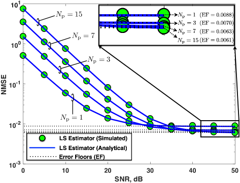
(a) $\beta=500$

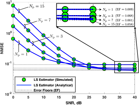
(b) $\beta=5000$

Figure 6: NMSE of LS PN-affected-channel estimator as a function of $\mathsf{SNR}$ for $\beta\in\{500,5000\}$ and $\mathcal{P}_{\rm d}=\{1,3,7,15\}$. Also shown are the error floors corresponding to the elements in $\mathcal{P}_{\rm d}$. The error floors are obtained by the NMSE expression in (47) with $\mathsf{SNR}=\infty$.

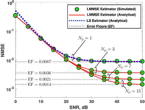
(a) $\beta=500$

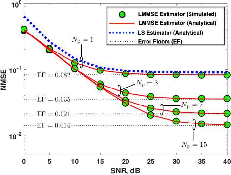
(b) $\beta=5000$

Figure 7: NMSE of LMMSE PN-affected-channel estimator as a function of $\mathsf{SNR}$ for $\beta\in\{500,5000\}$ and $\mathcal{P}_{\rm d}=\{1,3,7,15\}$. For comparison, the NMSE curve of LS estimator corresponding to $N_{\rm p}=1$ (dotted blue line) is included. Also shown are the error floors corresponding to the elements in $\mathcal{P}_{\rm d}$. The error floors are obtained by the NMSE expression in (48) with $\mathsf{SNR}=\infty$.

Remark 1.

(NMSE behavior for PN-affected-channel estimation): The LMMSE estimator with the second-order statistics of PN spectrum achieves better NMSE performance as increasing $N_{\rm p}$. One remarkable observation is that the LS estimator has different NMSE behavior depending on the SNR range. At low SNRs, the NMSE increases with $N_{\rm p}$ while it is the opposite at high SNRs. To look at the NMSE in the low and high SNR regimes, we approximate the NMSE of LS estimator (47) as follows.

$${\mathsf{NMSE}}_{{\rm p},{\mathsf{ls}}}\approx{\mathsf{NMSE}}_{{\rm p},{\mathsf{ls}}}^{\mathsf{app}}=\frac{1-\mathsf{P}_{\rm dom}+N_{\rm p}/\mathsf{SNR}}{\mathsf{P}_{\rm dom}},$$ (50)

where ${\mathsf{P}}_{\rm dom}\triangleq\mathbb{E}\big{\{}{\sum_{i\in\mathcal{P}}}{\|P_{i}\|_{2}^{2}}\big{\}}$ as the power sum of the $N_{\rm p}$ dominant PN components. The NMSE in the low and high SNR regimes, respectively, are

$$\lim_{{\mathsf{SNR}}\to\infty}{\mathsf{NMSE}}_{{\rm p},\mathsf{ls}}^{\mathsf{app}}=\frac{1-{\mathsf{P}}_{\rm dom}}{{\mathsf{P}}_{\rm dom}},\text{and}$$ (51)

$$\lim_{{\mathsf{SNR}}\to 0}{\mathsf{NMSE}}_{{\rm p},\mathsf{ls}}^{\mathsf{app}}=\frac{N_{\rm p}/{\mathsf{P}}_{\rm dom}}{\mathsf{SNR}}.$$ (52)

The NMSE at high SNRs (51) obviously decreases with $N_{\rm p}$. For the low SNR regime, let us define the numerator in (52) as $f(\gamma)\triangleq N_{\rm p}/{\mathsf{P}_{\rm dom}}$. This is an increasing function of the approximation order $\gamma$, i.e., $f(\gamma)^{\prime}>0$ for all $\gamma\geq 1$, translating into an NMSE degradation as $N_{\rm p}$ increases.

To validate our analysis, we compare the NMSE expressions for LS/LMMSE PN-affected-channel estimation (47) and (48) with the simulation result in Figs. 6-7. For the numerical evaluation, the following parameters are assumed: $N=4096$, $B=$245.76\text{\,}\mathrm{MHz}$$, $\Delta f=$60\text{\,}\mathrm{kHz}$$, which corresponds to one 3GPP NR signaling resource block to support communication at mmWave frequencies [35]. Also, we consider the set of dominant PN components $\mathcal{P}_{\rm d}=\{1,3,7,15\}$ and two kinds of 3-$\mathrm{dB}$ linewidth $\beta\in\{500,5000\}$ ($\mathrm{H}\mathrm{z}$) as LO parameters. The PN model that we adopt for the numerical evaluation is illustrated in Fig. 8. Both have severe PN spectrum compared to the one in conventional transceivers [8]. Unless otherwise stated, the same settings are assumed for numerical evaluation in this paper. As shown in Figs. 6-7, the agreement is excellent for all SNR and $N_{\rm p}$ values. Furthermore, it shows that the NMSE behavior follows the analysis in Remark 1.

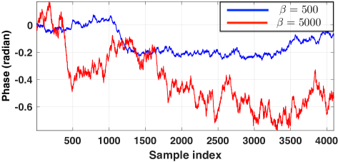
(a) Phase-noise trajectories (time domain)

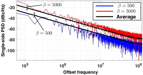
(b) Power spectrum density (frequency domain)

Figure 8: Phase-noise trajectories (one OFDM symbol with $N=4096$) and power spectrum density of free running oscillators, with $\beta=\{500,5000\}$, respectively. (simulated)

IV-B NMSE of ICI-free channel

The NMSE for ICI-free-channel estimation is

$${\mathsf{NMSE}}_{{\rm c},q}\triangleq\frac{\mathbb{E}[\|\hat{\mathbf{h}}_{{\rm If},q}-\tilde{\mathbf{h}}_{\rm If}\|_{2}^{2}]}{\mathbb{E}[\|\tilde{\mathbf{h}}_{\rm If}\|_{2}^{2}]},\;\;q\in\{{\mathsf{ls}},{\mathsf{lmmse}}\}.$$ (53)

From (53), the NMSEs of the LS and LMMSE ICI-free-channel estimators can be derived, respectively, as

$$\begin{split}{\mathsf{NMSE}}_{{\rm c},\mathsf{ls}}&=\frac{{\rm tr}\{\mathbf{R}_{\tilde{\mathbf{y}}\tilde{\mathbf{y}}}-\mathbf{R}_{\tilde{\mathbf{h}}\tilde{\mathbf{h}}}\}}{{\rm tr}\{\mathbf{R}_{\tilde{\mathbf{h}}\tilde{\mathbf{h}}}\}}\\ &=\frac{{\rm tr}\big{\{}\bar{G}\{1+(1/\mathsf{SNR})\}\mathbf{I}_{N_{\rm c}}-\bar{G}(1-\sigma_{\varepsilon}^{2})\mathbf{I}_{N_{\rm c}}\big{\}}}{{\rm tr}\{\bar{G}(1-\sigma_{\varepsilon}^{2})\mathbf{I}_{N_{\rm c}}\}}\\ &=\frac{N_{\rm c}\bar{G}\{1+(1/\mathsf{SNR})-1+\sigma_{\varepsilon}^{2}\}}{N_{\rm c}\bar{G}(1-\sigma_{\varepsilon}^{2})}=\frac{\frac{1}{\mathsf{SNR}}+\sigma_{\varepsilon}^{2}}{1-\sigma_{\varepsilon}^{2}},\text{and}\end{split}$$ (54)

$$\begin{split}{\mathsf{NMSE}}_{{\rm c},\mathsf{lmmse}}&=\frac{{\rm tr}\big{\{}\mathbf{R}_{\tilde{\mathbf{h}}\tilde{\mathbf{h}}}-\mathbf{R}_{\tilde{\mathbf{h}}\tilde{\mathbf{y}}}\mathbf{R}_{\tilde{\mathbf{y}}\tilde{\mathbf{y}}}^{-1}\mathbf{R}_{\tilde{\mathbf{y}}\tilde{\mathbf{h}}}\big{\}}}{{\rm tr}\{\mathbf{R}_{\tilde{\mathbf{h}}\tilde{\mathbf{h}}}\}}\\ &=\frac{{\rm tr}\Big{\{}\bar{G}(1-\sigma_{\varepsilon}^{2})\mathbf{I}_{N_{\rm c}}-\frac{\{\bar{G}(1-\sigma_{\varepsilon}^{2})\}^{2}}{\bar{G}\{1+(1/\mathsf{SNR})\}}(\mathbf{X}_{\rm f}^{\rm c})^{\rm H}\mathbf{X}_{\rm f}^{\rm c}\Big{\}}}{{\rm tr}\{\bar{G}(1-\sigma_{\varepsilon}^{2})\mathbf{I}_{N_{\rm c}}\}}\\ &=\frac{{\rm tr}\Big{\{}\bar{G}(1-\sigma_{\varepsilon}^{2})\Big{\{}1-\frac{\bar{G}(1-\sigma_{\varepsilon}^{2})}{\bar{G}\{1+(1/\mathsf{SNR})\}}\Big{\}}\mathbf{I}_{N_{\rm c}}\Big{\}}}{{\rm tr}\{\bar{G}(1-\sigma_{\varepsilon}^{2})\mathbf{I}_{N_{\rm c}}\}}\\ &=\frac{N_{\rm c}\bar{G}(1-\sigma_{\varepsilon}^{2})\Big{\{}1-\frac{1-\sigma_{\varepsilon}^{2}}{\{1+(1/\mathsf{SNR})\}}\Big{\}}}{N_{\rm c}\bar{G}(1-\sigma_{\varepsilon}^{2})}\\ &=\frac{\sigma_{\varepsilon}^{2}+(1/\mathsf{SNR})}{1+(1/\mathsf{SNR})}=\frac{1+\sigma_{\varepsilon}^{2}\mathsf{SNR}}{1+\mathsf{SNR}},\end{split}$$ (55)

where ${\mathbf{R}}_{\tilde{\mathbf{y}}\tilde{\mathbf{y}}}\triangleq\mathbb{E}\{\tilde{\mathbf{y}}_{\rm If}\tilde{\mathbf{y}}_{\rm If}^{\rm H}\}$, ${\mathbf{R}}_{\tilde{\mathbf{h}}\tilde{\mathbf{h}}}\triangleq\mathbb{E}\{\tilde{\mathbf{h}}_{\rm If}\tilde{\mathbf{h}}_{\rm If}^{\rm H}\}$, and ${\mathbf{R}}_{\tilde{\mathbf{h}}\tilde{\mathbf{y}}}\triangleq\mathbb{E}\{\tilde{\mathbf{h}}_{\rm If}\tilde{\mathbf{y}}_{\rm If}^{\rm H}\}$. Both NMSE expressions (54) and (55) can be formulated by only the average SNR and the effective-error variance.

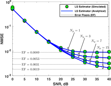
(a) $\beta=500$

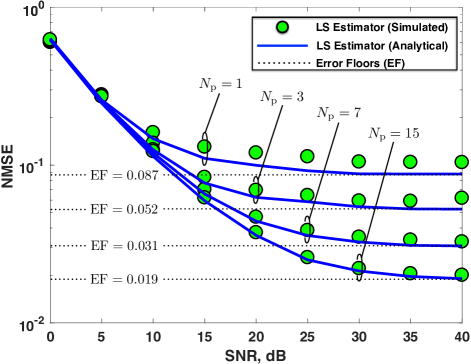
(b) $\beta=5000$

Figure 9: NMSE of LS ICI-free-channel estimator as a function of $\mathsf{SNR}$ for $\beta\in\{500,5000\}$ and $\mathcal{P}_{\rm d}=\{1,3,7,15\}$. Also shown are the error floors corresponding to the elements in $\mathcal{P}_{\rm d}$. The error floors are obtained by the NMSE expression in (54) with $\mathsf{SNR}=\infty$.

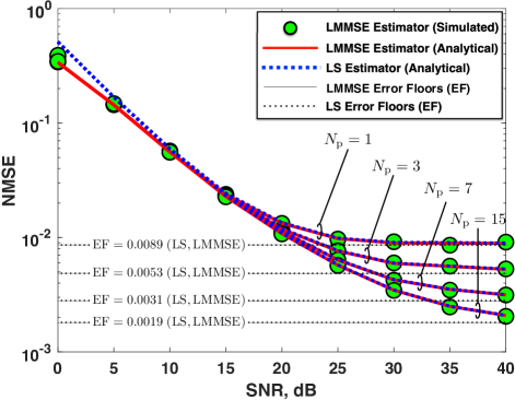
(a) $\beta=500$

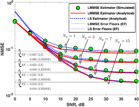
(b) $\beta=5000$

Figure 10: NMSE of LMMSE ICI-free-channel estimator as a function of $\mathsf{SNR}$ for $\beta\in\{500,5000\}$ and $\mathcal{P}_{\rm d}=\{1,3,7,15\}$. For comparison, the NMSE curves of LS estimator corresponding to the elements in $\mathcal{P}_{\rm d}$ (dotted blue line) are included. Also shown are the error floors corresponding to the elements in $\mathcal{P}_{\rm d}$. The error floors are obtained by (56) and (57), respectively.

Remark 2.

(NMSE floor of ICI-free-channel estimation): To present the NMSE floor of ICI-free-channel estimation, which bounds the achievable NMSE for linear estimators, let us look at the NMSEs in the high SNR regime. The NMSEs of LS/LMMSE ICI-free-channel estimators are lower-bounded by, respectively, i.e., ${\mathsf{NMSE}}_{{\rm c},q}\geq{\mathsf{NMSE}}_{{\rm c},q}^{\mathsf{lb}},\;q\in\{\mathsf{ls},\mathsf{lmmse}\}$,

$${\mathsf{NMSE}}_{{\rm c},\mathsf{ls}}^{\mathsf{lb}}=\lim_{{\mathsf{SNR}}\to\infty}{\mathsf{NMSE}}_{{\rm c},\mathsf{ls}}=\frac{\sigma_{\varepsilon}^{2}}{1-\sigma_{\varepsilon}^{2}},\text{and}$$ (56)

$${\mathsf{NMSE}}_{{\rm c},\mathsf{lmmse}}^{\mathsf{lb}}=\lim_{{\mathsf{SNR}}\to\infty}{\mathsf{NMSE}}_{{\rm c},\mathsf{lmmse}}=\sigma_{\varepsilon}^{2}.$$ (57)

In the case where the effective-error variance is small enough ($\sigma_{\varepsilon}^{2}\ll 1$), the lower bound of LS ICI-free-channel estimation (56) can be approximated as ${\mathsf{NMSE}}_{{\rm c},\mathsf{ls}}^{\mathsf{lb}}\approx\sigma_{\varepsilon}^{2}$, resulting in the same NMSE floor as the LMMSE estimator.

Comparisons of the NMSE expressions for LS/LMMSE ICI-free-channel estimation (54) and (55) with their simulation results are shown in Fig. 9-10. In the numerical evaluation, we used the LMMSE PN-affected-channel estimator. All figures have good agreements. The NMSE gap between LS and LMMSE estimators decreases as the SNR increases. In Fig. 10(a), it is observed that he LS and LMMSE NMSE floors are equal (rounded to fourth decimal place), as analyzed in Remark 2. However, in the more severe PN case ($\beta=5000$), higher effective-error variance arises, translating into a gap between LS and LMMSE NMSE floors shown in Fig. 10(b).

TABLE I: Computational complexity comparison.

		Estimation		Compensation
		Phase Noise	Wireless Channel	Phase Noise
Proposed¶	LS	$\mathcal{O}(0)$	$\mathcal{O}(N_{\rm c})$	$\mathcal{O}(NN_{\rm p})$
	LMMSE	$\mathcal{O}\big{(}N_{\rm p}^{2}(N_{\rm p}+1)\big{)}$	$\mathcal{O}(N_{\rm c}^{2})$
[41]†		$\mathcal{O}(N_{\rm p}^{3}+NL)$	$\mathcal{O}\big{(}N(N_{\rm p}+L)\big{)}$	$\mathcal{O}(NN_{\rm p})$
[43]		$\mathcal{O}(N_{\rm it}N^{3})$‡		$\mathcal{O}(N)$
[44]		$\mathcal{O}(N^{2}{\rm{log}_{2}}{N}+N_{\rm it}N)$‡	$\mathcal{O}(N)$	$\mathcal{O}(N)$

• In the proposed method, the PN-affected and ICI-free channels are applied instead of PN and wireless channel, respectively.

• $L$ denotes the number of effective channel taps in time domain.

• $N_{\rm it}$ denotes the number of iterations required.

V Pilot Overhead and Complexity Analysis

Our proposed algorithm translates into a practical PN estimation/compensation for mmWave OFDM systems. To derive this, we address the pilot-overhead and the computational complexity of our proposed method.

V-A Pilot Overhead Analysis

Recall that the resource allocation in each $\mathcal{S}$ ($|\mathcal{S}|=NN_{\rm ct}$) is identical where $\mathcal{S}$ is a set of coherence blocks across $N$ subcarriers as illustrated in Fig. 5. The pilot overhead is defined as $\rho_{\rm oh}\triangleq N_{\rm tp}/NN_{\rm ct}$ where $N_{\rm tp}$ is the total number of pilots. The following theorem provides the minimum pilot-overhead of the proposed algorithm.

Theorem 4.

Supposing a set of system parameters $\{N,N_{\rm ct},N_{\rm c},N_{\rm p}\}$, the minimum pilot-overhead for the PN-affected- and ICI-free-channel estimation is

$$\rho_{\rm oh}=\frac{N_{\rm ct}(2N_{\rm p}-1)+(N_{\rm c}-1)}{NN_{\rm ct}}.$$ (58)

Proof.

Consider the allocation of PN- and CH-dedicated pilots in the $\mathcal{S}$. It is shown in Theorem 1 that $(2N_{\rm p}-1)$ PN-dedicated pilots are required to estimate $N_{\rm p}$ PN-affected-channel coefficients. The PN-affected-channel estimation for each OFDM symbol leads the allocation of $N_{\rm ct}(2N_{\rm p}-1)$ PN-dedicated pilots in the $\mathcal{S}$. Recall that $(N_{\rm c}-1)$ CH-dedicated pilots are additionally needed for ICI-free-channel estimation over $N_{\rm ct}$ OFDM symbols. Hence (58) can be clearly derived. ∎

We provide an example below to help the understanding of how much the pilot overhead for our proposed algorithm is, as compared to the conventional cellular systems.

Example 4 (Comparison with the Cell-Specific Reference Symbol Overhead of Conventional Cellular Systems): In this example, let us consider a set of parameters in Long-Term Evolution (LTE) systems supporting $20\text{\,}\mathrm{MHz}$ channel bandwidth: $N=1200$, $N_{\rm ct}=7$, $N_{\rm c}=100$. We assume that one Cell-Specific Reference Symbol (CRS) is allocated for a resource block, i.e., $N_{\rm tp}=N_{\rm c}$. Based on this parameter set, therefore, the CRS overhead $\rho_{\rm oh,crs}\triangleq N_{\rm c}/(NN_{\rm ct})$ is $1.19\text{\,}\%$, which does not include the overhead for PN estimation. Consider the set of the number of dominant PN components $\mathcal{P}_{\rm d}=\{1,3,7,15\}$. The corresponding minimum pilot-overhead ratios from (58) are $1.26\text{\,}\%$, $1.60\text{\,}\%$, $2.26\text{\,}\%$, and $3.60\text{\,}\%$, respectively. These are quite reasonable values for the practical use of our algorithm.

V-B Computational Complexity Analysis

In this subsection, we investigate the computational complexity of the PN-affected-/ICI-free-channel estimation and the ICI suppression (PN compensation). Since the LS PN-affected-channel estimator (23) is an identity matrix, no computation is required for obtaining $\hat{\mathbf{f}}_{{\bar{\rm p}},\mathsf{ls}}$. The LMMSE PN-affected-channel estimator (24) and the matrix-vector multiplication (25) have a complexity of respectively $\mathcal{O}\big{(}N_{\rm p}^{3}\big{)}$ and $\mathcal{O}\big{(}N_{\rm p}^{2}\big{)}$, leading to a total complexity in the order of $\mathcal{O}\big{(}N_{\rm p}^{2}(N_{\rm p}+1)\big{)}$. According to (43) – (45), the complexity order of the LS/LMMSE ICI-free-channel estimation is $\mathcal{O}(N_{\rm c})$ and $\mathcal{O}(N_{\rm c}^{2})$, respectively. As described in Section III-C, the PN compensation in the proposed method is performed in the frequency domain. Recall that the PN effect is a circular convolution process in the frequency domain. Hence the PN compensation process is the deconvolution of the received signal and the PN estimate in frequency. It results in a complexity of $\mathcal{O}(N^{2})$. Since the length-$N$ PN-affected-channel estimate $\hat{\mathbf{f}}_{\rm p}$ includes only $N_{\rm p}$ nonzero values, the deconvolution (33) has a complexity $\mathcal{O}({NN_{\rm p}})$.

The complexity comparison with existing work on low-complexity PN estimation and compensation is shown in Table  I. From the relation $N\gg N_{\rm p},N_{\rm c}$, the proposed method has lower complexity for both PN and channel estimation than the existing solutions. Let us consider a total complexity, including joint PN/channel estimation and PN compensation, with mmWave system parameters. For example, if $N=4096$, $N_{\rm p}=7$, $N_{\rm c}=100$, $L=5$, and $N_{\rm it}=1$, the proposed method with the LMMSE estimation obtains a reduction of $2.53\times$, $(1.76\times 10^{6})\times$, and $(5.15\times 10^{3})\times$, respectively, in the total complexity, as compared to [41, 43, 44]. Furthermore, all of these existing solutions require a full-pilot OFDM symbol to perform joint PN and channel estimation, which leads to significant pilot overhead to tackle the problem of fast-varying PN estimation.

VI Trade-Off Analysis

This section uses BER and throughput to study the trade-off between performance and pilot-overhead. For the numerical evaluation, the following parameters are used: $N=4096$, $\Delta f=$60\text{\,}\mathrm{kHz}$$, and $N_{\rm c}=275$, which corresponds to one 3GPP NR signaling to support communication at mmWave frequency [35]. Also, we consider the set of dominant phase-noise components $\mathcal{P}_{\rm d}\in\{1,3,7,15\}$ and two kinds of 3-$\rm{dB}$ linewidth $\beta\in\{500,5000\}$.

VI-A Bit-Error Rate Performance

Fig. 11 shows the BER performance for an OFDM system transmitting uncoded 16- quadrature amplitude modulation (QAM). The BER curves of $N_{\rm p}$-perfect PN compensation serve as a benchmark, where it is assumed that $N_{\rm p}\in\{3,7\}$ dominant PN components are perfectly known, and able to be used for the compensation. The performance curve without PN is used as another benchmark for comparison. As illustrated in Fig. 11(a), the proposed method has quite good BER performance by using the estimation of even only three significant PN components when $\beta=500$. In case of $N_{\rm p}\in\{3,7\}$, it is shown that there is around $3\hskip 1.00006pt{\rm dB}$ difference between perfect $N_{\rm p}$-perfect phase-noise compensation and proposed method at a BER of $10^{-3}$. In comparison with no PN case, there is around $3.5\hskip 1.00006pt{\rm dB}$ and $5\hskip 1.00006pt{\rm dB}$, respectively, for $N_{\rm p}\in\{3,7\}$, at the same BER level. Also, it is observed that, when $N_{\rm p}>3$, the performance improvements by the proposed method is relatively small. It means that most of PN energy is focused in three dominant PN components in the $\beta=500$ case. Whereas the BER performance shown in Fig. 11(b) ($\beta=5000$ ) is largely improved, as more number of dominant PN components is considered. For example, as $N_{\rm p}\in\{1,3,7,15\}$ increases, their BERs at the $30\hskip 1.00006pt{\rm dB}$ SNR level, are 0.089, 0.048, 0.02, and 0.007, respectively. We can tell that there is more room to improve the BER performance by the use of pilot-overhead, as compared to the $\beta=500$.

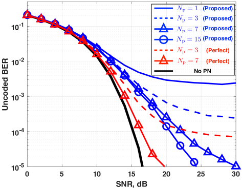
(a) $\beta=500$

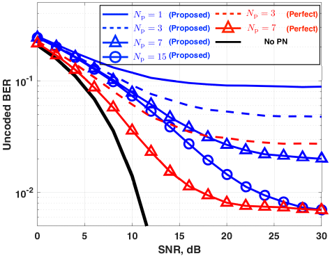
(b) $\beta=5000$

Figure 11: BER performance of the proposed solutions (blue), $N_{\rm p}$-perfect PN compensation (red), and no PN case (black) with $\beta\in\{500,5000\}$.

VI-B Throughput versus Pilot-Overhead Trade-Off

To study the trade-off between performance and pilot-overhead, we define the throughput based on 3GPP terminologies, as follows:

$${\mathsf{THP}}=(1-\rho_{\rm oh})\times\frac{N_{\rm c}\times N_{\rm re}\times N_{\mathsf{ofdm}}}{T_{\mathsf{slot}}}\times M_{\mathsf{qam}}\times(1-\mathsf{BER}),$$ (59)

where $N_{\rm c}$ and $N_{\rm re}$ are the number of resource blocks, resource elements in a resource block, respectively; $N_{\mathsf{ofdm}}$ is the number of OFDM symbols per slot, $T_{\mathsf{slot}}$ the slot duration, $M_{\mathsf{qam}}$ a modulation order per resource element, $\mathsf{BER}$ the average BER. For the numerical evaluation with (59), the following parameters are assumed: $N_{\rm re}=12$, $N_{\mathsf{ofdm}}=14$, $T_{\mathsf{slot}}=$0.25\text{\,}\mathrm{ms}$$, $M_{\mathsf{qam}}=4$, which also corresponds to one 3GPP NR signaling resource block to support communication at mmWave frequency [35]. Fig. 12 shows the throughput performance as a function of SNR. From (58), the pilot-overhead $\rho_{\rm oh}$, according to $N_{\rm p}\in\mathcal{P}_{\rm d}$, is 1.22 %, 1.34 %, 1.58 %, and 2.06 %, respectively. When $\beta=5000$, the higher-order PN approximation and its estimation lead to the better throughput performance although the more pilot-overhead is required. On the other hand, when $\beta=500$, the estimation of three dominant PN components, i.e., $N_{\rm p}=3$, results in better throughput performance than the others, in the SNR range more than $6\hskip 1.00006pt{\rm dB}$. At the high SNRs, the throughput with $N_{\rm p}=3$ is around $5.2\hskip 1.00006pt{\rm{Mbits/s}}$ higher than the one with $N_{\rm p}=15$, while the $N_{\rm p}=15$ case has around $24.4\hskip 1.00006pt{\rm{Mbits/s}}$ higher throughput, as compared to the $N_{\rm p}=3$. From these results, it is found that higher-order PN estimation does not guarantee better throughput performance due to the increase of the pilot-overhead.

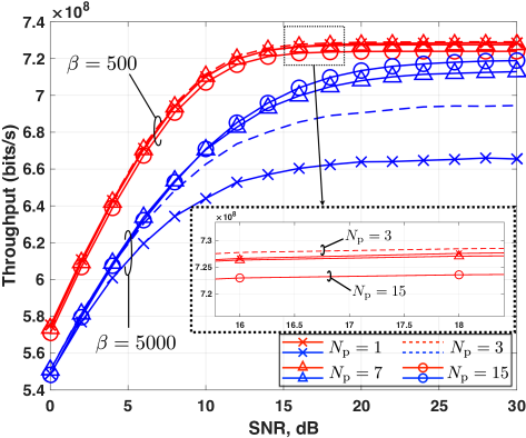
Figure 12: Trade-off between throughput and pilot-overhead with $\mathcal{P}_{\rm d}=\{1,3,7,15\}$ and $\beta\in\{500,5000\}$.

Although the pilot-overhead effort leads to the throughput improvement when $\beta=5000$, the high-order approximation of PN spectrum, e.g., $N_{\rm p}=7$ or $15$, may not always be required. The computational complexity of PN-affected-channel estimation is a function of $N_{\rm p}$, i.e., $\mathcal{O}\big{(}N_{\rm p}^{2}(N_{\rm p}+1)\big{)}$ with LMMSE estimator. In case where the throughput difference is marginal according to $N_{\rm p}$, the lowest $N_{\rm p}$ could be selected to reduce the complexity, if not for throughput-sensitive applications. For example, when $\beta=5000$, the PN spectrum approximation with $N_{\rm p}=1$ could be considered for a SNR of less than about $2\hskip 1.00006pt{\rm dB}$, and $N_{\rm p}=3$ for a SNR of $2$ - $5\hskip 1.00006pt{\rm dB}$.

VII Conclusion

Practically suppressing the effect of PN is a critical aspect of mmWave communication systems to realize its potential benefits. This paper has outlined a novel framework for PN compensation on OFDM systems, which uses LS/LMMSE estimators and pilot-assisted transmission. Our main conclusion is that the large coherence bandwidth in mmWave bands and an approximation of the PN spectrum enable low-complexity PN compensation with a reasonable pilot-overhead, which leads to a very efficient solution for the severe PN problem. Further, we have derived analytically tractable expressions for the NMSE performance of our proposed framework, and studied the trade-off between performance and pilot-overhead. These expressions and trade-off analysis offer an insight into an appropriate approximation of the PN spectrum, according to the SNR and PN environments.

$${\mathbf{\Phi}_{\rm ici,{\gamma}}^{\rm p}}=\begin{bmatrix}P_{N-N_{\rm b}}&P_{N-N_{\rm b}-1}&P_{N-N_{\rm b}-2}&\cdots&P_{N_{\rm a}+1}&P_{N_{\rm a}}\\ P_{N-N_{\rm b}+1}&P_{N-N_{\rm b}}&P_{N-N_{\rm b}-1}&\cdots&P_{N_{\rm a}+2}&P_{N_{\rm a}+1}\\ \vdots&\vdots&\vdots&\cdots&\vdots&\vdots\\ P_{N-N_{\rm b}+(N_{\rm p}-1)}&P_{N-N_{\rm b}+(N_{\rm p}-2)}&P_{N-N_{\rm b}+(N_{\rm p}-3)}&\cdots&P_{N_{\rm a}+N_{\rm p}}&P_{N_{\rm a}+(N_{\rm p}-1)}\end{bmatrix}.$$ (64)

Appendix A Proof of Theorem 1

From (19), we have the generalized form of $\mathbf{y}_{\rm f}^{\rm p}$ with respect to $\gamma$-order approximation as follows:

$$\mathbf{y}_{\rm f}^{\rm p}={\mathbf{X}_{\rm f,\gamma}^{\rm p}}{\mathbf{f}_{\bar{\rm{p}}}}+{\mathbf{w}}_{\gamma}^{\rm p},$$ (60)

where ${\mathbf{w}}^{\rm p}_{\gamma}=[W_{\gamma,0}^{\rm p},W_{\gamma,1}^{\rm p},\cdots,W_{\gamma,N_{\rm p}-1}^{\rm p}]\in\mathbb{C}^{N_{\rm p}\times 1}$ is the ICI by the $\gamma$-order-approximation error plus AWGN in $\mathbf{y}_{\rm f}^{\rm p}$. The element set in the $\mathbf{X}_{{\rm f},\gamma}^{\rm p}$ is $\{X_{k}^{\rm p}\}_{k=0}^{2N_{\rm p}-2}$, which means that $(2N_{\rm p}-1)$ PN-dedicated pilots are required to estimate $N_{\rm p}$ PN-affected-channel components. Regarding each observation in $\mathbf{y}_{\rm f}^{\rm p}$, the $N_{\rm p}$ PN-dedicated pilots are multiplied with the $\mathbf{f}_{\bar{\rm p}}$. The remaining $(N_{\rm p}-1)$-pilot, however, combines with higher-order PN components than $\gamma$, resulting in being involved in $\mathbf{w}_{\gamma}^{\rm p}$. To meet two conditions for PN-dedicated-pilot pattern, which are the ICI minimization and ${\rm rank}(\mathbf{X}_{\rm f,\gamma}^{\rm p})=N_{\rm p}$, we employ the fact that the diagonal term $X_{\rm 2\gamma}^{\rm p}$ in $\mathbf{X}_{\rm f,\gamma}^{\rm p}$ does not belong to $\mathbf{w}_{\gamma}^{\rm p}$ and can be used for making the full rank of $\mathbf{X}_{\rm f,\gamma}^{\rm p}$. Hence, a non-zero pilot symbol is allocated for $X_{\rm 2\gamma}^{\rm p}$ and zero-pilot for the remainder to minimize the ICI, leading to the optimal PN-dedicated pilot matrix (21).

Appendix B LMMSE Estimator for PN-Affected Channel

The LMMSE PN-affected-channel estimator is defined as

$${\mathbf{Q}}_{\mathsf{lmmse}}={\mathbf{R}}_{\mathbf{f}\mathbf{y}}{{\mathbf{R}}_{\mathbf{y}\mathbf{y}}}^{-1},$$ (61)

where ${\mathbf{R}}_{\mathbf{f}\mathbf{y}}=\mathbb{E}\{{\mathbf{f}_{\bar{\rm p}}}({\mathbf{y}_{\rm f}^{\rm p}})^{\rm H}\}$ is the cross-covariance matrix between ${\mathbf{f}_{\bar{\rm p}}}$ and ${\mathbf{y}_{\rm f}^{\rm p}}$, ${\mathbf{R}}_{\mathbf{y}\mathbf{y}}=\mathbb{E}\{{\mathbf{y}_{\rm f}^{\rm p}}({\mathbf{y}_{\rm f}^{\rm p}})^{\rm H}\}$ the autocorrelation matrix of ${\mathbf{y}_{\rm f}^{\rm p}}$. Substituting (21) in Theorem 1 into (60) , we have

$$\begin{split}{\mathbf{R}}_{\mathbf{f}\mathbf{y}}&=\mathbb{E}\{{\mathbf{f}_{\bar{\rm p}}}({\mathbf{X}_{\rm f,\gamma}^{\rm p}}{\mathbf{f}_{\bar{\rm p}}}+{\mathbf{w}_{\gamma}^{\rm p}})^{\rm H}\}\\ &=\mathbb{E}\{{\mathbf{f}_{\bar{\rm p}}}{\mathbf{f}_{\bar{\rm p}}}^{\rm H}\}+\underbrace{\mathbb{E}\{{\mathbf{f}_{\bar{\rm p}}}({\mathbf{E}_{\gamma}^{\rm p}}{\mathbf{x}_{\rm f}}+{\mathbf{z}_{\rm f}})^{\rm H}\}}_{\mathbf{0}_{N_{\rm p}\times N_{\rm p}}}\\ &\stackrel{{\scriptstyle\text{(a)}}}{{=}}\underbrace{\mathbb{E}\{\|\alpha\|_{2}^{2}\}}_{1}\underbrace{\mathbb{E}\{\bar{\mathbf{p}}_{{\rm f},\gamma}(\bar{\mathbf{p}}_{{\rm f},\gamma})^{\rm H}\}}_{\mathbf{R}_{\mathbf{p}\mathbf{p}}^{\gamma}}=\mathbf{R}_{\mathbf{p}\mathbf{p}}^{\gamma},\end{split}$$ (62)

$$\begin{split}{\mathbf{R}}_{\mathbf{y}\mathbf{y}}&=\mathbb{E}\{({\mathbf{f}_{\bar{\rm p}}}+{\mathbf{w}_{\gamma}^{\rm p}})({\mathbf{f}_{\bar{\rm p}}}+{\mathbf{w}_{\gamma}^{\rm p}})^{\rm H}\}\\ &=\mathbf{R}_{\mathbf{p}\mathbf{p}}^{\gamma}+\mathbb{E}\{{\mathbf{E}_{\gamma}^{\rm p}}{\mathbf{x}_{\rm f}}{{\mathbf{x}_{\rm f}}^{\rm H}}({\mathbf{E}_{\gamma}^{\rm p}})^{\rm H}\}+\underbrace{\mathbb{E}\{{\mathbf{z}_{\rm f}}{\mathbf{z}_{\rm f}^{\rm H}}\}}_{\sigma_{z}^{2}{\mathbf{I}_{N_{\rm p}}}}\\ &=\mathbf{R}_{\mathbf{p}\mathbf{p}}^{\gamma}+\underbrace{\mathbb{E}\{\tilde{\mathbf{\Phi}}_{{\rm f},\gamma}^{\rm p}({\tilde{\mathbf{\Phi}}_{{\rm f},\gamma}^{\rm p})^{\rm H}}\}}_{\mathbf{R}_{\mathbf{ici}}}+\sigma_{z}^{2}{\mathbf{I}_{N_{\rm p}}}\\ &=\mathbf{R}_{\mathbf{p}\mathbf{p}}^{\gamma}+\mathbf{R}_{\mathbf{ici}}+(1/{\mathsf{SNR}}){\mathbf{I}_{N_{\rm p}}}.\end{split}$$ (63)

where ${\mathbf{E}}_{\gamma}^{\rm p}\in\mathbb{C}^{N_{\rm p}\times N}$ is the $\gamma$-order-approximation-error matrix in $\mathbf{y}_{\rm f}^{\rm p}$, $\tilde{\mathbf{\Phi}}_{{\rm f},\gamma}^{\rm p}=[\mathbf{\Phi}_{{\rm ici},\gamma}^{\rm p}\;\;\mathbf{0}_{N_{\rm p}\times(2N_{\rm p}-1)}]\in\mathbb{C}^{N_{\rm p}\times N}$. The $\mathbf{\Phi}_{{\rm ici},\gamma}^{\rm p}\in\mathbb{C}^{N_{\rm p}\times(N-2N{\rm p}+1)}$ is given in (64) at the bottom of this page, where $N_{\rm a}\triangleq\frac{N_{\rm p}+1}{2}$ and $N_{\rm b}\triangleq\frac{3N_{\rm p}-1}{2}$.

$$\begin{split}\mathbf{R}_{\tilde{\mathbf{h}}\tilde{\mathbf{y}}}&=\mathbb{E}\{\tilde{\mathbf{h}}_{\rm If}(\tilde{\mathbf{H}}_{\rm If}\mathbf{x}_{\rm f}^{\rm c}+\tilde{\mathbf{\Upsilon}}_{\rm off}\mathbf{H}_{\rm If}\mathbf{x}_{\rm f}+\tilde{\mathbf{z}}_{\rm f})^{\rm H}\}\\ &=\mathbb{E}\{\tilde{\mathbf{h}}_{\rm If}\tilde{\mathbf{h}}_{\rm If}^{\rm H}\}(\mathbf{X}_{\rm f}^{\rm c})^{\rm H}+\underbrace{\mathbb{E}\{\tilde{\mathbf{h}}_{\rm If}(\tilde{\mathbf{\Upsilon}}_{\rm off}\mathbf{H}_{\rm If}\mathbf{x}_{\rm f})^{\rm H}\}}_{\mathbf{0}_{N_{\rm c}\times N_{\rm c}}}+\underbrace{\mathbb{E}\{\tilde{\mathbf{h}}_{\rm If}\tilde{\mathbf{z}}_{\rm f}^{\rm H}\}}_{\mathbf{0}_{N_{\rm c}\times N_{\rm c}}}\\ &=\bar{G}(1-\sigma_{\varepsilon}^{2})(\mathbf{X}_{\rm f}^{\rm c})^{\rm H}\end{split}$$ (72)

$$\begin{split}\mathbf{R}_{\tilde{\mathbf{y}}\tilde{\mathbf{y}}}&=\mathbb{E}\Big{\{}\big{(}\tilde{\mathbf{D}}_{N}\{\mathbf{I}_{N}-\alpha\mathbf{G}_{\rm p}\mathbf{E}_{\rm t,eff}\}\mathbf{D}_{N}^{\rm H}\mathbf{H}_{\rm If}\mathbf{x}_{\rm f}+\tilde{\mathbf{z}}_{\rm f}\big{)}\big{(}\tilde{\mathbf{D}}_{N}\{\mathbf{I}_{N}-\alpha\mathbf{G}_{\rm p}\mathbf{E}_{\rm t,eff}\}\mathbf{D}_{N}^{\rm H}\mathbf{H}_{\rm If}\mathbf{x}_{\rm f}+\tilde{\mathbf{z}}_{\rm f}\big{)}^{\rm H}\Big{\}}\\ &=\frac{1}{\|\alpha\|_{2}^{2}}\mathbb{E}\big{\{}\tilde{\mathbf{D}}_{N}\{\mathbf{I}_{N}-\alpha\mathbf{G}_{\rm p}\mathbf{E}_{\rm t,eff}\}\{\mathbf{I}_{N}-\alpha\mathbf{G}_{\rm p}\mathbf{E}_{\rm t,eff}\}^{\rm H}\tilde{\mathbf{D}}_{N}^{\rm H}\big{\}}+\mathbb{E}\{\tilde{\mathbf{z}}_{\rm f}\tilde{\mathbf{z}}_{\rm f}^{\rm H}\}\\ &=\frac{1}{\|\alpha\|_{2}^{2}}\mathbb{E}\big{\{}\tilde{\mathbf{D}}_{N}\{\alpha\mathbf{G}_{\rm p}\mathbf{\Phi}_{\rm t}\}\{\alpha\mathbf{G}_{\rm p}\mathbf{\Phi}_{\rm t}\}^{\rm H}\tilde{\mathbf{D}}_{N}^{\rm H}\big{\}}+\tilde{\mathbf{D}}_{N}\mathbf{G}_{\rm p}\mathbf{D}_{N}^{\rm H}\underbrace{\mathbb{E}\{\mathbf{z}_{\rm f}\mathbf{z}_{\rm f}^{\rm H}\}}_{\sigma_{z}^{2}\mathbf{I}_{N}}\mathbf{D}_{N}\mathbf{G}_{\rm p}^{\rm H}\tilde{\mathbf{D}}_{N}^{\rm H}\\ &=\tilde{\mathbf{D}}_{N}\mathbf{G}_{\rm p}\mathbf{G}_{\rm p}^{\rm H}\tilde{\mathbf{D}}_{N}^{\rm H}+\sigma_{z}^{2}\tilde{\mathbf{D}}_{N}\mathbf{G}_{\rm p}\mathbf{G}_{\rm p}^{\rm H}\tilde{\mathbf{D}}_{N}^{\rm H}=(1+\sigma_{z}^{2})\tilde{\mathbf{D}}_{N}\mathbf{G}_{\rm p}\mathbf{G}_{\rm p}\tilde{\mathbf{D}}_{N}^{\rm H}\\ &=\bar{G}\big{\{}1+(1/\mathsf{SNR})\big{\}}\mathbf{I}_{N_{\rm c}}\end{split}$$ (73)

Appendix C Proof of Theorem 2

The equivalent time-domain representation of $\hat{\mathbf{f}}_{\rm p}$ and $\mathbf{e}_{\rm f,app}$ can be described as follows:

$$\hat{\mathbf{f}}_{\rm p}=\alpha(\mathbf{p}_{\rm f,\gamma}+\mathbf{e}_{\rm f,est})\longleftrightarrow\mathbf{g}_{\rm p}=\alpha(\mathbf{p}_{\rm t,\gamma}+\mathbf{e}_{\rm t,est}),$$ (65)

$$\mathbf{e}_{\rm f,app}=\mathbf{p}_{\rm f}-\mathbf{p}_{\rm f,\gamma}\longleftrightarrow\mathbf{e}_{\rm t,app}=\mathbf{p}_{\rm t}-\mathbf{p}_{\rm t,\gamma}.$$ (66)

where $\mathbf{p}_{\rm t}\triangleq\sqrt{N}\mathbf{D}_{N}^{\rm H}\mathbf{p}_{\rm f}=[e^{j\phi_{0}},e^{j\phi_{1}},\cdots,e^{j\phi_{N-1}}]^{\rm T}$, $\mathbf{p}_{\rm t,\gamma}\triangleq\sqrt{N}\mathbf{D}_{N}^{\rm H}\mathbf{p}_{\rm f,\gamma}=[p_{0},p_{1},\cdots,p_{N-1}]^{\rm T}$, $\mathbf{e}_{\rm t,est}\triangleq\sqrt{N}{\mathbf{D}}_{N}^{\rm H}\mathbf{e}_{\rm f,est}=[E_{\rm t,0}^{\rm est},E_{\rm t,1}^{\rm est},\cdots,E_{{\rm t},N-1}^{\rm est}]^{\rm T}\in\mathbb{C}^{N\times 1}$. The deconvolution output-vector of $\mathbf{y}_{\rm If}$ and $\hat{\mathbf{f}}_{\rm p}$ is

$$\begin{split}\mathbf{y}_{\rm If}&=\mathbf{D}_{N}\underbrace{\Big{\{}\big{\{}{\rm diag}\big{\{}g_{{\rm p},n}\big{\}}_{n=0}^{N-1}\big{\}}^{-1}\Big{\}}}_{\mathbf{G}_{\rm p}}\mathbf{D}_{N}^{\rm H}\mathbf{y}_{\rm f}\\ &=\mathbf{D}_{N}\Big{\{}\frac{1}{\alpha}\big{\{}\underbrace{{\rm diag}\{p_{n}\}_{n=0}^{N-1}}_{\triangleq\mathbf{\Phi}_{{\rm t},\gamma}}+\underbrace{{\rm diag}\{E_{{\rm t},n}^{\rm est}\}_{n=0}^{N-1}}_{\triangleq\mathbf{E}_{\rm t,est}}\big{\}}^{-1}\Big{\}}\mathbf{D}_{N}^{\rm H}\mathbf{y}_{\rm f}\\ &\stackrel{{\scriptstyle\text{(a)}}}{{=}}\mathbf{D}_{N}\Big{\{}\frac{1}{\alpha}\big{\{}\mathbf{\Phi}_{{\rm t},\gamma}^{-1}-\mathbf{\Phi}_{{\rm t},\gamma}^{-1}\big{\{}\mathbf{\Phi}_{{\rm t},\gamma}^{-1}+\mathbf{E}_{\rm t,est}^{-1}\big{\}}^{-1}\mathbf{\Phi}_{{\rm t},\gamma}^{-1}\big{\}}\Big{\}}\mathbf{D}_{N}^{\rm H}\mathbf{y}_{\rm f}\\ &\stackrel{{\scriptstyle\text{(b)}}}{{=}}\frac{1}{\alpha}\mathbf{D}_{N}\Big{\{}\mathbf{I}_{N}-\big{\{}\mathbf{\Phi}_{{\rm t},\gamma}+\mathbf{E}_{\rm t,est}\big{\}}^{-1}\mathbf{E}_{\rm t,est}\Big{\}}\mathbf{\Phi}_{{\rm t},\gamma}^{-1}\mathbf{D}_{N}^{\rm H}\mathbf{y}_{\rm f}\\ &=\frac{1}{\alpha}\mathbf{D}_{N}\big{\{}\mathbf{I}_{N}-\alpha\mathbf{G}_{\rm p}\mathbf{E}_{\rm t,est}\big{\}}\mathbf{y}_{\rm d}\\ &=\underbrace{\frac{1}{\alpha}\mathbf{H}_{\rm f}}_{\triangleq\mathbf{H}_{\rm If}}\mathbf{x}_{\rm f}+\bar{\mathbf{\Upsilon}}\mathbf{H}_{\rm If}\mathbf{x}_{\rm f}+\bar{\mathbf{z}}_{\rm f}=\{\mathbf{I}+\bar{\mathbf{\Upsilon}}\}\mathbf{H}_{\rm If}\mathbf{x}_{\rm f}+\bar{\mathbf{z}}_{\rm f},\end{split}$$ (67)

where (a) and (b) follow from the matrix identity $(\mathbf{A}+\mathbf{B})^{-1}=\mathbf{A}^{-1}-\mathbf{A}^{-1}(\mathbf{A}^{-1}+\mathbf{B}^{-1})^{-1}\mathbf{A}^{-1}$ and $(\mathbf{A}^{-1}+\mathbf{B}^{-1})^{-1}=\mathbf{A}(\mathbf{A}+\mathbf{B})^{-1}\mathbf{B}$, respectively;

$$\begin{split}\mathbf{y}_{\rm d}&=\mathbf{\Phi}_{{\rm t},\gamma}^{-1}\mathbf{D}_{N}^{\rm H}\mathbf{y}_{\rm f}=\mathbf{\Phi}_{{\rm t},\gamma}^{-1}\mathbf{D}_{N}^{\rm H}\Big{\{}\mathbf{F}_{\gamma}\mathbf{x}_{\rm f}+\mathbf{E}_{\gamma}\mathbf{x}_{\rm f}+\mathbf{z}_{\rm f}\Big{\}}\\ &=\mathbf{\Phi}_{{\rm t},\gamma}^{-1}\mathbf{D}_{N}^{\rm H}\Big{\{}\mathbf{\Phi}_{{\rm f},\gamma}\mathbf{H}_{\rm f}\mathbf{x}_{\rm f}+\underbrace{\{\mathbf{\Phi}_{\rm f}-\mathbf{\Phi}_{\rm f,\gamma}\}}_{\triangleq\tilde{\mathbf{\Phi}}_{\rm f,\gamma}}\mathbf{H}_{\rm f}\mathbf{x}_{\rm f}+\mathbf{z}_{\rm f}\Big{\}}\\ &\stackrel{{\scriptstyle\text{(c)}}}{{=}}\mathbf{\Phi}_{{\rm t},\gamma}^{-1}\mathbf{D}_{N}^{\rm H}\Big{\{}\mathbf{D}_{N}\mathbf{\Lambda}_{\Phi}\mathbf{D}_{N}^{\rm H}\mathbf{H}_{\rm f}\mathbf{x}_{\rm f}+\mathbf{D}_{N}\tilde{\mathbf{\Lambda}}_{\Phi}\mathbf{D}_{N}^{\rm H}\mathbf{H}_{\rm f}\mathbf{x}_{\rm f}+\mathbf{z}_{\rm f}\Big{\}}\\ &=\underbrace{\mathbf{\Phi}_{{\rm t},\gamma}^{-1}\mathbf{\Lambda}_{\Phi}}_{\mathbf{I}_{N}}\mathbf{D}_{N}^{\rm H}\mathbf{H}_{\rm f}\mathbf{x}_{\rm f}+\mathbf{\Phi}_{{\rm t},\gamma}^{-1}\tilde{\mathbf{\Lambda}}_{\Phi}\mathbf{D}_{N}^{\rm H}\mathbf{H}_{\rm f}\mathbf{x}_{\rm f}+\mathbf{\Phi}_{{\rm t},\gamma}^{-1}\mathbf{D}_{N}^{\rm H}\mathbf{z}_{\rm f}\\ &=\mathbf{D}_{N}^{\rm H}\mathbf{H}_{\rm f}\mathbf{x}_{\rm f}+\mathbf{\Phi}_{{\rm t},\gamma}^{-1}\tilde{\mathbf{\Lambda}}_{\Phi}\mathbf{D}_{N}^{\rm H}\mathbf{H}_{\rm f}\mathbf{x}_{\rm f}+\mathbf{\Phi}_{{\rm t},\gamma}^{-1}\mathbf{D}_{N}^{\rm H}\mathbf{z}_{\rm f},\end{split}$$ (68)

$$\begin{split}\bar{\mathbf{\Upsilon}}&=\mathbf{D}_{N}\Big{\{}\big{\{}\mathbf{I}_{N}-\alpha\mathbf{G}_{\rm p}\mathbf{E}_{\rm t,est}\big{\}}\Big{\{}\mathbf{\Phi}_{{\rm t},\gamma}^{-1}\tilde{\mathbf{\Lambda}}_{\Phi}\Big{\}}-\alpha\mathbf{G}_{\rm p}\mathbf{E}_{\rm t,est}\Big{\}}\mathbf{D}_{N}^{\rm H}\\ &\stackrel{{\scriptstyle\text{(d)}}}{{=}}\mathbf{D}_{N}\Big{\{}\big{\{}\mathbf{I}_{N}-\alpha\mathbf{G}_{\rm p}\mathbf{E}_{\rm t,est}\big{\}}\Big{\{}\mathbf{\Phi}_{{\rm t},\gamma}^{-1}\mathbf{E}_{\rm t,app}\Big{\}}-\alpha\mathbf{G}_{\rm p}\mathbf{E}_{\rm t,est}\Big{\}}\mathbf{D}_{N}^{\rm H}\\ &=\mathbf{D}_{N}\Big{\{}\underbrace{\big{\{}\mathbf{I}_{N}-\alpha\mathbf{G}_{\rm p}\mathbf{E}_{\rm t,est}\big{\}}\mathbf{\Phi}_{{\rm t},\gamma}^{-1}}_{\alpha\mathbf{G}_{\rm p}}\mathbf{E}_{\rm t,app}-\alpha\mathbf{G}_{\rm p}\mathbf{E}_{\rm t,est}\Big{\}}\mathbf{D}_{N}^{\rm H}\\ &=\alpha\mathbf{D}_{N}\mathbf{G}_{\rm p}\underbrace{\Big{\{}\mathbf{E}_{\rm t,app}-\mathbf{E}_{\rm t,est}\Big{\}}}_{-\mathbf{E}_{\rm t,eff}}\mathbf{D}_{N}^{\rm H}\\ &=-\alpha\mathbf{D}_{N}\mathbf{G}_{\rm p}\mathbf{E}_{\rm t,eff}\mathbf{D}_{N}^{\rm H}=-\mathbf{\Upsilon}.\end{split}$$ (69)

In (68) and (69), (c) and (d) follow from Lemma 2 ($\mathbf{\Lambda}_{\Phi}=\mathbf{\Phi}_{{\rm t},\gamma}$, $\tilde{\mathbf{\Lambda}}_{\Phi}=\mathbf{E}_{\rm t,app}$); $\mathbf{E}_{\rm t,app}$ is the diagonal matrix with entries from $\mathbf{e}_{\rm t,app}$ on its main diagonal.

$$\begin{split}\bar{\mathbf{z}}_{\rm f}&=\frac{1}{\alpha}\mathbf{D}_{N}\Big{\{}\{\mathbf{I}_{N}-\alpha\mathbf{G}_{\rm p}\mathbf{E}_{\rm t,est}\}\mathbf{\Phi}_{{\rm t},\gamma}^{-1}\Big{\}}\mathbf{D}_{N}^{\rm H}\mathbf{z}_{\rm f}\\ &=\frac{1}{\alpha}\mathbf{D}_{N}\Big{\{}\alpha\mathbf{G}_{\rm p}\Big{\}}\mathbf{D}_{N}^{\rm H}\mathbf{z}_{\rm f}\\ &=\mathbf{D}_{N}\mathbf{G}_{\rm p}\mathbf{D}_{N}^{\rm H}\mathbf{z}_{\rm f}.\\ \end{split}$$ (70)

Appendix D LMMSE Estimator for ICI-Free Channel

The LMMSE estimator for ICI-free channel vector $\tilde{\mathbf{h}}_{\rm If}$ is defined as

$${\mathbf{V}}_{\mathsf{lmmse}}={\mathbf{R}}_{\tilde{\mathbf{h}}\tilde{\mathbf{y}}}{\mathbf{R}}_{\tilde{\mathbf{y}}\tilde{\mathbf{y}}}^{-1},$$ (71)

where ${\mathbf{R}}_{\tilde{\mathbf{h}}\tilde{\mathbf{y}}}=\mathbb{E}\{\tilde{\mathbf{h}}_{\rm If}\tilde{\mathbf{y}}_{\rm If}^{\rm H}\}$ is the cross-covariance matrix between $\tilde{\mathbf{h}}_{\rm If}$ and $\tilde{\mathbf{y}}_{\rm If}$; ${\mathbf{R}}_{\tilde{\mathbf{y}}\tilde{\mathbf{y}}}=\mathbb{E}\{\tilde{\mathbf{y}}_{\rm If}\tilde{\mathbf{y}}_{\rm If}^{\rm H}\}$ is the autocorrelation matrix of $\tilde{\mathbf{y}}_{\rm If}$. Based on (42), the ${\mathbf{R}}_{\tilde{\mathbf{h}}\tilde{\mathbf{y}}}$ and ${\mathbf{R}}_{\tilde{\mathbf{y}}\tilde{\mathbf{y}}}$ are represented as (72) and (73), respectively, in the bottom of this page, where $\bar{G}\triangleq\frac{1}{N}\sum_{n=0}^{N-1}\{\|1/g_{{\rm p},n}\|_{2}^{2}\}$ is the mean of absolute-squared diagonal coefficients in $\mathbf{G}_{\rm p}$.

Appendix E Autocorrelation Coefficients of $\mathbf{R}_{\mathbf{pp}}^{\gamma}$ and $\mathbf{R}_{\mathbf{ici}}^{\gamma}$

The autocorrelation coefficient $R_{k,\ell}$ in $\mathbf{R}_{\mathbf{pp}}$ is [47]

$$\begin{split}R_{k,\ell}&=\mathbb{E}\{P_{k}P_{\ell}^{*}\}\\ &={\frac{1}{N^{2}}}\mathbb{E}\Bigg{\{}{\sum_{m=0}^{N-1}\sum_{n=0}^{N-1}}{e^{j(\phi_{m}-\phi_{n})}}{e^{-j{\frac{2\pi}{N}}(mk-n\ell)}}\Bigg{\}}\\ &={\frac{1}{N^{2}}}{\sum_{m=0}^{N-1}\sum_{n=0}^{N-1}}\mathbb{E}\{{e^{j\Delta\phi_{m,n}}}\}{e^{-j{\frac{2\pi}{N}}(mk-n\ell)}}\\ &\stackrel{{\scriptstyle\text{(a)}}}{{=}}{\frac{1}{N^{2}}}{\sum_{m=0}^{N-1}\sum_{n=0}^{N-1}}\underbrace{\{{e^{-\pi\beta|m-n|T_{\rm s}}}\}}_{\triangleq\psi_{m,n}}{e^{-j{\frac{2\pi}{N}}(mk-n\ell)}}\end{split}$$ (74)

where (a) is determined using the moment generating function of $\Delta\phi_{m,n}$. The autocorrelation coefficient $R_{k,\ell}^{\rm{ici}}$ of $\mathbf{R}_{\mathbf{ici}}^{\gamma}$ is

$$\begin{split}R_{k,\ell}^{\rm ici}={\sum_{i=N_{\rm a}+k}^{N-N_{\rm b}+k}}{R_{i,i+(\ell-k)}}\end{split}$$ (75)

References

- [1] M. Chung, L. Liu, O. Edfors, and F. Sheikh, “Phase noise compensation for OFDM systems exploiting coherence bandwidth,” in Proc. IEEE Int. Workshop on Signal Processing Advances in Wireless Communications (SPAWC), pp. 1–5, Jul. 2019.
- [2] T. S. Rappaport, S. Sun, R. Mayzus, H. Zhao, Y. Azar, K. Wang, G. N. Wong, J. K. Schulz, M. Samimi, and F. Gutierrez, “Millimeter wave mobile communications for 5G cellular: It will work!” IEEE Access, vol. 1, pp. 335–349, 2013.
- [3] J. G. Andrews, S. Buzzi, W. Choi, S. V. Hanly, A. Lozano, A. C. K. Soong, and J. C. Zhang, “What will 5G be?” IEEE Journal on Selected Areas in Communications, vol. 32, no. 6, pp. 1065–1082, 2014.
- [4] M. Chung, L. Liu, A. Johansson, M. Nilsson, O. Zander, Z. Ying, F. Tufvesson, and O. Edfors, “Millimeter-wave massive MIMO testbed with hybrid beamforming,” in Proc. Asilomar Conference on Signals, Systems, and Computers, pp. 1–5, Nov. 2020.
- [5] M. Chung, L. Liu, A. Johansson, S. Gunnarsson, M. Nilsson, Z. Ying, O. Zander, K. Samanta, C. Clifton, T. Koimori, S. Morita, S. Taniguchi, F. Tufvesson, and O. Edfors, “LuMaMi28: Real-time millimeter-wave massive MIMO systems with antenna selection,” Sep. 2021, [Online] Available: https://arxiv.org/pdf/2109.03273.pdf.
- [6] W. P. Robins, Phase noise in signal sources: theory and applications. vol.9. IET, 1984.
- [7] M. Chung, H. Prabhu, F. Sheikh, O. Edfors, and L. Liu, “Low-complexity fully-digital phase noise suppression for millimeter-wave systems,” in Proc. IEEE Int. Symp. on Circ. and Sys. (ISCAS), pp. 1–5, Oct. 2020.
- [8] A. A. Zaidi, R. Baldemair, H. Tullberg, H. Bjorkegren, L. Sundstrom, J. Medbo, C. Kilinc, and I. Da Silva, “Waveform and numerology to support 5G services and requirements,” IEEE Communications Magazine, vol. 54, no. 11, pp. 90–98, Nov. 2016.
- [9] G. D. Surabhi, M. K. Ramachandran, and A. Chockalingam, “OTFS modulation with phase noise in mmWave communications,” in Proc. IEEE Vehicular Technology Conference (VTC), pp. 1–5, May 2019.
- [10] N. Grimwood, T. Dean, and A. Goldsmith, “Robustness of FDM-FDCP modulation to phase noise in millimeter wave systems,” in Proc. Asilomar Conference on Signals, Systems, and Computers, pp. 264–268, Feb 2019.
- [11] T. Pollet, M. Van Bladel, and M. Moeneclaey, “BER sensitivity of OFDM systems to carrier frequency offset and Wiener phase noise,” IEEE Transactions on Communications, vol. 43, no. 234, pp. 191–193, Feb. 1995.
- [12] H. Steendam, M. Moeneclaey, and H. Sari, “The effect of carrier phase jitter on the performance of orthogonal frequency-division multiple-access systems,” IEEE Transactions on Communications, vol. 46, no. 4, pp. 456–459, Apr. 1998.
- [13] A. G. Armada, “Understanding the effects of phase noise in orthogonal frequency division multiplexing (OFDM),” IEEE Transactions on Broadcasting, vol. 47, no. 2, pp. 153–159, Jun. 2001.
- [14] S. Wu and Y. Bar-Ness, “OFDM systems in the presence of phase noise: consequences and solutions,” IEEE Transactions on Communications, vol. 52, no. 11, pp. 1988–1996, Nov. 2004.
- [15] L. Piazzo and P. Mandarini, “Analysis of phase noise effects in OFDM modems,” IEEE Transactions on Communications, vol. 50, no. 10, pp. 1696–1705, Dec. 2002.
- [16] L. Tomba, “On the effect of Wiener phase noise in OFDM systems,” IEEE Transactions on Communications, vol. 46, no. 5, pp. 580–583, May 1998.
- [17] P. Mathecken, T. Riihonen, N. Tchamov, S. Werner, M. Valkama, and W. R., “Characterization of OFDM radio link under pll-based oscillator phase noise and multipath fading channel,” IEEE Transactions on Communications, vol. 60, no. 6, pp. 1479–1485, Jun. 2012.
- [18] K. Zhong, Y. Wu, and S. Li, “Signal detection for OFDM-based virtual MIMO systems under unknown doubly selective channels, multiple interferences and phase noises,” IEEE Transactions on Wireless Communications, vol. 12, no. 10, pp. 5309–5321, Sep. 2013.
- [19] A. Pitarokoilis, S. K. Mohammed, and E. G. Larsson, “Uplink performance of time-reversal MRC in massive MIMO systems subject to phase noise,” IEEE Transactions on Wireless Communications, vol. 14, no. 2, pp. 711–723, Sep 2015.
- [20] R. Krishnan, M. R. Khanzadi, N. Krishnan, Y. Wu, A. Graell i Amat, T. Eriksson, and R. Schober, “Linear massive MIMO precoders in the presence of phase noise–A large-scale analysis,” IEEE Transactions on Vehicular Technology, vol. 65, no. 5, pp. 3057–3071, May 2016.
- [21] E. Björnson, M. Matthaiou, and M. Debbah, “Massive MIMO with non-ideal arbitrary arrays: Hardware scaling laws and circuit-aware design,” IEEE Transactions on Wireless Communications, vol. 14, no. 8, pp. 4353–4368, Apr. 2015.
- [22] Q. Zhang, T. Q. S. Quek, and S. Jin, “Scaling analysis for massive mimo systems with hardware impairments in rician fading,” IEEE Transactions on Wireless Communications, vol. 17, no. 7, pp. 4536–4549, Jul. 2018.
- [23] S. Jacobsson, U. Gustavsson, G. Durisi, and C. Studer, “Massive MU-MIMO-OFDM uplink with hardware impairments: Modeling and analysis,” in Proc. Asilomar Conference on Signals, Systems, and Computers, pp. 1829–1835, Oct. 2018.
- [24] P. Robertson and S. Kaiser, “Analysis of the effects of phase-noise in orthogonal frequency division multiplex (OFDM) systems,” in Proc. IEEE International Conference on Communications (ICC), pp. 1652–1657, Jun. 1995.
- [25] A. G. Armada and M. Calvo, “Phase noise and sub-carrier spacing effects on the performance of an OFDM communication system,” IEEE Communications Letters, vol. 2, no. 1, pp. 11–13, Jan. 1998.
- [26] R. A. Casas, S. L. Biracree, and A. E. Youtz, “Time domain phase noise correction for OFDM signals,” IEEE Transactions on Broadcasting, vol. 48, no. 3, pp. 230–236, Sep. 2002.
- [27] G. Liu and W. Zhu, “Compensation of phase noise in OFDM systems using an ICI reduction scheme,” IEEE Transactions on Broadcasting, vol. 50, no. 4, pp. 399–407, Dec. 2004.
- [28] S. Suyama, H. Suzuki, K. Fukawa, and J. Izumi, “Iterative receiver employing phase noise compensation and channel estimation for millimeter-wave OFDM systems,” IEEE Journal on Selected Areas in Communications, vol. 27, no. 8, pp. 1358–1366, Sep. 2009.
- [29] H. Mehrpouyan, A. A. Nasir, S. D. Blostein, T. Eriksson, G. K. , Karagiannidis, and T. Svensson, “Joint estimation of channel and oscillator phase noise in MIMO systems,” IEEE Transactions on Signal Processing, vol. 60, no. 9, pp. 4790–4807, Sep. 2012.
- [30] R. Wang, H. Mehrpouyan, M. Tao, and Y. Hua, “Channel estimation, carrier recovery, and data detection in the presence of phase noise in OFDM relay systems,” IEEE Transactions on Wireless Communications, vol. 15, no. 2, pp. 1186–1205, Feb. 2016.
- [31] A. Kreimer and D. Raphaeli, “Efficient low complexity phase noise resistant iterative joint phase estimation and decoding algorithm,” IEEE Transactions on Communications, vol. 66, no. 9, pp. 4199–4210, Apr. 2018.
- [32] H. Huang, W. G. J. Wang, and J. He, “Phase noise and frequency offset compensation in high frequency MIMO-OFDM system,” in Proc. IEEE International Conference on Communications (ICC), pp. 1280–1285, Jun. 2015.
- [33] K. Wang, L. M. A. Jalloul, and A. Gomaa, “Phase noise compensation using limited reference symbols in 3GPP lte downlink,” Jun. 2018, [Online] Available: https://arxiv.org/abs/1711.10064.
- [34] Y. Qi, M. Hunukumbure, H. Nam, H. Yoo, and S. Amuru, “On the phase tracking reference signal (PT-RS) design for 5G new radio (NR),” Jul. 2018, [Online] Available: https://arxiv.org/abs/1807.07336.
- [35] 3rd Generation Partnership Project (3GPP), Physical channels and modulation (Release 15), 3GPP TS 38.211 V15.3.0, Sep. 2018.
- [36] T. Marzetta, “Noncooperative cellular wireless with unlimited numbers of base station antennas,” IEEE Transactions on Wireless Communications, vol. 9, no. 11, pp. 3590–3600, Nov. 2010.
- [37] F. Rusek, D. Persson, B. K. Lau, E. G. Larsson, T. L. Marzetta, O. Edfors, and F. Tufvesson, “Scaling up MIMO: Opportunities and challenges with very large arrays,” IEEE Signal Processing Magazine, vol. 30, no. 1, pp. 40–60, Jan. 2013.
- [38] E. Björnson, E. G. Larsson, and T. L. Marzetta, “Massive MIMO: Ten myths and one critical question,” IEEE Communications Magazine, vol. 54, no. 2, pp. 114–123, Feb. 2016.
- [39] A. Demir, A. Mehrotra, and J. Roychowdhury, “Phase noise in oscillators: A unifying theory and numerical methods for characterization,” IEEE Transactions on Circuits and Systems I: Fundamental Theory and Applications, vol. 47, no. 5, pp. 655–674, May 2000.
- [40] A. V. Oppenheim, R. W. Schafer, and J. R. Buck, Discrete-time signal processing. Prentice Hall, 1989.
- [41] P. Rabiei, W. Namgoong, and N. Al-Dhahir, “A non-iterative technique for phase noise ICI mitigation in packet-based OFDM systems,” IEEE Transactions on Signal Processing, vol. 58, no. 11, pp. 5945–5950, Nov. 2010.
- [42] P. Mathecken, T. Riihonen, S. Werner, and R. Wichman, “Phase noise estimation in OFDM: Utilizing its associated spectral geometry,” IEEE Transactions on Signal Processing, vol. 64, no. 8, pp. 1999–2012, Apr. 2016.
- [43] Q. Zou, A. Tarighat, and A. H. Sayed, “Compensation of phase noise in OFDM wireless systems,” IEEE Transactions on Signal Processing, vol. 55, no. 11, pp. 5407–5424, Nov. 2007.
- [44] Z. Wang, P. Babu, and D. P. Palomar, “Effective low-complexity optimization methods for joint phase noise and channel estimation in OFDM,” IEEE Transactions on Signal Processing, vol. 65, no. 12, pp. 3247–3260, Jun. 2017.
- [45] S. Hur, T. Kim, D. J. Love, J. V. Krogmeier, T. A. Thomas, and A. Ghosh, “Millimeter wave beamforming for wireless backhaul and access in small cell networks,” IEEE Transactions on Communications, vol. 61, no. 10, pp. 4391–4403, Oct. 2013.
- [46] S. M. Kay, Fundamentals of statistical signal processing. Prentice Hall PTR, 1993.
- [47] D. Petrovic, W. Rave, and G. Fettweis, “Effects of phase noise on OFDM systems with and without PLL: Characterization and compensation,” IEEE Transactions on Communications, vol. 55, no. 8, pp. 1607–1616, Aug. 2007.
- [48] P. J. Davis, Circulant matrices. American Mathematical Soc., 2012.
- [49] Y. G. Li, J. H. Winters, and N. R. Sollenberger, “MIMO-OFDM for wireless communications: signal detection with enhanced channel estimation,” IEEE Transactions on Communications, vol. 50, no. 9, pp. 1471–1477, Nov. 2002.
- [50] H. Yin, D. Gesbert, M. Filippou, and Y. Liu, “A coordinated approach to channel estimation in large-scale multiple-antenna systems,” IEEE Journal on Selected Areas in Communications, vol. 31, no. 2, pp. 264–273, Jan. 2013.
- [51] N. Shariati, E. Björnson, M. Bengtsson, and M. Debbah, “Low-complexity polynomial channel estimation in large-scale MIMO with arbitrary statistics,” IEEE Journal of Selected Topics in Signal Processing, vol. 8, no. 5, pp. 815–830, Apr. 2014.
- [52] R. Hamila, Ö. Özdemir, and N. Al-Dhahir, “Beamforming OFDM performance under joint phase noise and I/Q imbalance,” IEEE Transactions on Vehicular Technology, vol. 65, no. 5, pp. 2978–2989, May 2016.
- [53] P. Liu, S. Jin, T. Jiang, Q. Zhang, and M. Matthaiou, “Pilot power allocation through user grouping in multi-cell massive MIMO systems,” IEEE Transactions on Communications, vol. 65, no. 4, pp. 156–1574, Apr. 2017.
- [54] S. Sesia, I. Toufik, and M. Baker, LTE: the UMTS long term evolution. New York: John Wiley Sons, 2009.
- [55] M. K. Samimi and T. S. Rappaport, “Local multipath model parameters for generating 5G millimeter-wave 3GPP-like channel impulse response,” in Proc. IEEE European Conference on Antennas and Propagation, pp. 1–5, Apr. 2016.
- PN
- phase-noise
- mmWave
- millimeter-wave
- LO
- local oscillator
- CPE
- common phase error
- ICI
- inter-carrier interference
- SINR
- signal-to-interference-plus-noise ratio
- BER
- bit error rate
- PTRS
- Phase Tracking Reference Signal
- 3GPP
- 3rd Generation Partnership Project
- NR
- New Radio
- LS
- least-squares
- LMMSE
- linear minimum mean squared-error
- NMSE
- normalized mean squared-error
- SNR
- signal-to-noise ratio
- IDFT
- inverse discrete Fourier transform
- CP
- cyclic prefix
- MIMO
- multiple-input multiple-output
- QAM
- quadrature amplitude modulation
- OFDM
- orthogonal frequency-division multiplexing
- BS
- base station
- MMSE
- Minimum Mean Square Error
- MU-MIMO
- Multi-User MIMO
- MS
- Mobile Station
- DPC
- Dirty Paper Coding
- ZF
- Zero-Forcing
- MF
- Matched Filter
- VPU
- vector processing unit
- MSB
- Most Significant Bit
- WL
- Word Length
- FF
- Folding Factor
- FIFO
- First-In-First-Out
- MUI
- Multi-User Interference
- DNS
- Diagonal Neumann Series
- TNS
- Tri-diagonal Neumann series
- MAC
- Multiply-Accumulate
- CE
- constant envelope
- PE
- Processing Element
- PA
- Power Amplifier
- PAR
- Peak-to-Average Ratio
- CCDF
- Complementary Cumulative Distribution Function
- OBR
- Out-of-Band (ratio) Power
- SDNR
- Signal-to-distortion-plus-noise ratio
- IBO
- Input-Back-off
- OBO
- Output-Back-off
- ISI
- Inter-Symbol Interference
- MUI
- Multi-user interference
- LUT
- Look-Up-Table