Optimal tool path planning for 3D printing with spatio-temporal and thermal constraints

Abstract

In this paper, we address the problem of synthesizing optimal path plans in $2D$ subject to spatio-temporal and thermal constraints. Our solution consists of reducing the path planning problem to a Mixed Integer Linear Programming (MILP) problem. The challenge is in encoding the “implication” constraints in the path planning problem using only conjunctions that are permitted by the MILP formulation. Our experimental analysis using an implementation of the encoding in a Python toolbox demonstrates the feasibility of our approach in generating the optimal plans.

I INTRODUCTION

Path Planning [1, 2] is a classical problem in robotics that has been extensively investigated. In this paper, we focus on $2D$ path planning in the presence of spatio-temporal and thermal constraints to optimize for superior structural properties of printed $3D$ structures in the context of additive manufacturing.

Additive manufacturing or the $3D$ printing procedure broadly consists of placing material in $3$-dimensional space with the help of computer-controlled material delivery systems, and fusing new material onto either a printing platform or previously printed material. Few common additive manufacturing methods include Fused Filament Fabrication (FFF), Selective Laser Sintering (SLS) and Stereolithography (SLA). In this paper, we focus on FFF process, which is widely used due to its ease of customization and cost effectiveness. Broadly, the $3D$ printing procedure takes a $3D$ CAD model of a structure as input, and generates $2D$ projections of the models at different layer heights using a software called a “slicer”. The sequence of multiple $2$-dimensional layers are then printed to create a $3$-dimensional part. To print a particular layer, the printer uses $3$ computer-controlled motors, one for each axis, to precisely position a material extruder in $3D$ space which melts a filament in a heating chamber and extrudes (draws) onto the print bed or onto previously printed parts. It has been observed that structural properties of the printed parts are affected by the temperature profile during the printing [3].

In this paper, we focus on the $2D$ tool path planning, and our objective is to ensure that the printing pattern is covered by the printer in the least time, while at the same time maintaining the temperature between certain bounds. In particular, this requires us to consider the spatio-temporal heat evolution model in the planning problem. We consider a discrete setting, wherein the $2D$ print bed is divided into a finite number of cells, and the print pattern is specified by a subset of these cells. The problem is to synthesize a plan for the traversal of the printhead/nozzle with the constraint that the nozzle can move one unit along the $x$-axis or the $y$-axis in each time step. We also simplify/discretize the heat equation, and include that in our planning model.

Our broad approach to synthesizing the plan is to encode the optimal path planning problem into a Mixed Integer Linear Programming (MILP) problem, and use an off-the-shelf solver to obtain the optimal assignment to the variables from which a plan can be extracted. The challenge arises from the fact that a straightforward encoding of the constraints requires using “implications” while MILP only supports conjunctions of linear constraints. Hence, we need to choose appropriate variables and define appropriate linear constraints that can encode these “implications”. We have implemented the encoding and the extraction algorithms in a Python toolbox. We illustrate our procedure on an example, as well as report our experimental analysis which demonstrates the feasibility of the approach to synthesize optimal plans for spatio-temporal and thermal constraints.

The novelty of our work lies in the fact that while $2D$ path planning has been investigated extensively, it has not been studied in the context of spatio-temporal and thermal constraints that need to be considered to optimize for superior structural properties.

I-A Related Work

Coverage problem consists of generating a plan to cover a given area, which is closely related to printing problem, that requires covering a print region. Path planning problem for coverage have been investigated in  [4, 5, 6]. Optimal path planning has been extensively investigated in the context of minimizing the total distance travelled [7, 8, 9, 10, 11, 12, 13, 14, 15].

In the context of tool path planning for $3D$ printers, two classes of algorithms have been explored, namely, those that provide an optimal path to visit a set of points in a two dimensional plane, and those that traverse a set of print segments such that the total distance travelled along non-print segments is minimized. Several strategies for path generation have been explored that do not necessarily consider optimality including Raster  [16], ZigZag  [17], Contour  [18], Spiral  [19], and Fractal space curves  [20]. Optimal path planning for the first class of problems has been investigated based on modifications of the asymmetric travelling salesman problem [21]. The second class of problems have been investigated for different velocity profiles including constant velocity profiles [22] and triangular/trapezoidal velocity profiles  [23, 24, 25, 26]. Further, $3D$ path planning algorithms based on Eulerian tour checking algorithm known as Hierholzer’s algorithm [22], tour construction algorithm known as Frederickson’s algorithm  [23, 27], Christofides algorithm [23], and greedy $2$-Opt and greedy annealing algorithm [28], have been considered. While several of these algorithms focus on optimality of the $2D$/$3D$ path plans with respect to distance travelled, none of them optimize the plans for superior structural properties based on thermal constraints, which is the focus of this paper.

II Preliminaries

Let $\mathbb{R}$ denote the set of real numbers and $\mathbb{Z}$ the set of integers. Let $[n]$ denote the set $\{0,\cdots,n-1\}$. Given a sequence $\rho=a_{0}a_{1}a_{2}\cdots a_{k}$, $\rho(i)$ will denote the $i$-th element, namely, $a_{i}$, and $k$ will be the length of $\rho$. Given an $m\times n$ matrix $P$, we use $P(i,j)$ to denote the $j$-th element of the $i$-th row of $P$; the row numbers are $0,1,\cdots,m-1$ and the column numbers are $0,1,\cdots,n-1$.

III $2D$ path planning problem

In this section, we discuss the optimal $2D$ path planning problem under spatio-temporal and thermal constraints towards achieving superior structural properties, and formalize a discrete version of the problem.

III-A An overview

We focus on a $2D$ path planning problem that corresponds to printing a “slice” of a given $3D$ object. The print head can move in the $x$ and $y$ directions, and can extrude the print material during the movement. While the print head moves in continuous fragments, we consider a discrete version of the problem as a simplified first step to incorporate the spatio-temporal and thermal constraints required to print objects with superior structural properties. Hence, we divide the two dimensional plan into an $m\times n$ grid, and specify a subset of these cells as the print region as shown in Figure 1. It shows a $3\times 3$ grid partitioning the print bed (or a $2D$ layer) into $9$ cells, where the diagonal cells constitute the print pattern. We allow the print head to move to the adjacent cell either in the $x$-direction or in the $y$-direction in one time step, but not simultaneously in both directions.

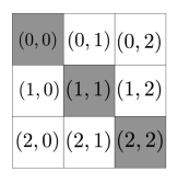
Figure 1: A $3\times 3$ bed with print region (gray)

The nozzle extrudes the material by heating the filament, hence, the print bed’s temperature increases at the point of extrusion of the material. The heat evolves in a spatio-temporal manner according to the heat equation, given by the following partial differential equation (PDE):

$$\frac{\partial{T}}{\partial{t}}=\alpha(\frac{\partial{{}^{2}T}}{\partial{x}^{2}}+\frac{\partial{{}^{2}T}}{\partial{y}^{2}})+u(x,y,t),$$ (1)

where $T(x,y,t)$ is the temperature at the position $(x,y)$ at time $t$, $\alpha$ is the thermal diffusivity, and $u(x,y,t)$ is the temperature applied at time $t$ to position $(x,y)$, which in our case will be the temperature of the extruded material. We consider a simple discrete model of the heat equation, wherein we replace the second derivatives $\frac{\partial{{}^{2}T}}{\partial{x}^{2}}$ and $\frac{\partial{{}^{2}T}}{\partial{y}^{2}}$ by their first derivatives $\frac{\partial{T}}{\partial{x}}$ and $\frac{\partial{T}}{\partial{y}}$, respectively. Further, we discretize $\frac{\partial{T}}{\partial{x}}$ and $\frac{\partial{T}}{\partial{y}}$. Note that $\frac{\partial{T}}{\partial{x}}$ can be approximated as $\frac{T(x+\Delta,y,t)-T(x,y,t)}{\Delta}$, for a given $\Delta$. By taking $\Delta$ to be $1$ (which corresponds to the next cell along the $x$-axis) we obtain $T(x+1,y,t)-T(x,y,t)$. Similarly, we can approximate the slope from the left, that is, take $\Delta=-1$, and we obtain $T(x,y,t)-T(x-1,y,t)$. We approximate the partial derivative by the average of the approximation from the left and the right and obtain $[T(x+1,y,t)-T(x,y,t)+T(x,y,t)-T(x-1,y,t)]/2=[T(x+1,y,t)-T(x-1,y,t)]/2$. Similarly, we approximate the partial derivative with respect to $y$ by $[T(x,y+1,t)-T(x,y-1,t)]/2$. Hence, we obtain the following difference equation approximating the heat evolution:

$$T(x,y,t+1)-T(x,y,t)=\alpha[T(x+1,y,t)-T(x-1,y,t)+$$

$$T(x,y+1,t)-T(x,y-1,t)]/2+u(x,y,t)$$ (2)

III-B Problem Formulation

We formalize the optimal tool path planning problem. Formally, the problem is specified using a printing scenario $\textit{S}=(m,n,\textit{P},\textit{T},\textit{T}_{l},\textit{T}_{u},\alpha,\textit{T}_{h})$, where:

• the bed is divided into an $m\times n$ grid of cells;

• P is an $m\times n$ matrix that specifies the printing pattern, that is, $\textit{P}(i,j)=1$ implies that the cell $(i,j)$ needs to be printed, and $\textit{P}(i,j)=0$ implies that cell $(i,j)$ does not need to be printed;

• T is an $m\times n$ matrix that specifies the initial temperature profile of the bed, that is, $\textit{T}(i,j)$ is a real number that specifies the temperature of the cell $(i,j)$ at the beginning of printing, that is, at time $0$;

• $\textit{T}_{l}$ and $\textit{T}_{u}$ provide lower and upper bounds on the temperature of the bed during the printing; and

• $\alpha$ and $\textit{T}_{h}$ are parameters for the temperature evolution model.

The objective is to find a plan such that the pattern is printed, the temperature constraints are maintained and the time to print is minimized. Two cells positions $(i,j)$ and $(i^{\prime},j^{\prime})$ are adjacent if either $i=i^{\prime}$ and $|j-j^{\prime}|=1$ or $j=j^{\prime}$ and $|i-i^{\prime}|=1$. A plan is a sequence of adjacent cells, that is, $\rho=\{(x_{k},y_{k})\}_{k\in[d]}$ such that $(x_{k+1},y_{k+1})$ is an adjacent cell of $(x_{k},y_{k})$, for all $k$. We refer to $(x_{k},y_{k})$ as the $k$-th cell visited by the plan. Let $\textit{Cost}(\rho)$ denote the distance travelled along $\rho$, that is, the length of $\rho$. An annotated plan is a pair $(\rho,\{u_{k}\}_{k\in[d]},\{\textit{T}_{k}\}_{k\in[d]})$, where $\rho$ is a plan of length $d$, $u_{k}\in\{0,1\}$ indicates if the nozzle is printing at the $k$-th time instance in the plan, and $\textit{T}_{k}(i,j)$ specifies the temperature of cell $(i,j)$ at time $k$. Our objective is to find an annotated path with minimum cost, such that the following conditions hold:

• Cover the pattern: For every $(i,j)$, if $P(i,j)=1$, then there is exactly one $k\in\{1,\cdots,d\}$ such that $\rho(k)=(i,j)$ and $b_{k}=1$; and if $P(i,j)=0$, then there is no $k\in\{1,\cdots,d\}$ such that $\rho(k)=(i,j)$ and $b_{k}=1$.

• Temperature evolution constraints: The temperature profile at time $k+1$ is related to that at time $k$ according to Equation (2). For all $(i,j)$, $\textit{T}_{0}(i,j)=\textit{T}(i,j)$, and

  $$\textit{T}_{k+1}(i,j)=\textit{T}_{k}(i,j)+\alpha([\textit{T}_{k}(i+1,j)-\textit{T}_{k}(i-1,j)]/2$$

  $$+[\textit{T}_{k}(i,j+1)-\textit{T}_{k}(i,j-1)]/2)+T_{h}u_{k}b_{k},$$ (3)

  where $b_{k}=1$ if $\rho(k)=(i,j)$, and $0$, otherwise. Note that if $(i,j)$ corresponds to a boundary cell, then some of the indices on the right are outside the range $[m]\times[n]$, we take those $\textit{T}_{k}(i,j)$ to be $0$ (or equivalently, eliminate those terms from the equation).

• Temperature bound constraints: The temperature always remains within the bounds $\textit{T}_{l}$ and $\textit{T}_{u}$. For all $i\in[m],j\in[n],k\in[d]$,

  $$\textit{T}_{l}\leq\textit{T}_{k}(i,j)\leq\textit{T}_{u}$$

We refer to an annotated path that satisfies the above conditions as valid.

IV Plan Synthesis using MILP

In this section, we provide a method to synthesize a plan to print a given pattern with a minimum length plan while satisfying the temperature constraints. Our broad approach is to encode the problem as a Mixed Integer Linear Programming (MILP) problem and to extract a plan from a satisfying valuation of the constraints. The challenge arises from the fact that a natural way to encode our problem involves implications, however, MILP only allows conjunctions, where as implication requires disjunction. Hence, we need to use a slightly involved encoding that avoids the implications. First, we provide an overview of MILP, and then we present our encoding.

IV-A MILP

Mixed Integer Linear Programming (MILP) refer to an optimization problem with linear objectives and linear constraints where the variables consist of a mixture of real and integer variables. Let $x=(x_{0},\cdots,x_{n-1})$ be a tuple of variables, where $I\subseteq[n]$ is a set of indices which correspond to integer variables, with the rest being real variables. The general form of MILP is given by:

$$\min c^{T}x$$

$$Ax\leq b,\ x\in\mathbb{R}^{n},\ x_{i}\in\mathbb{Z},\ \forall i\in I$$

Here $c^{T}x$ represents a linear objective function, $Ax\leq b$ represents a finite number of linear constraints over the variables $x$, where the constants $c$, $A$ and $b$ are rationals. The problem is to find a real valuation for all the variables $x$, with the additional restriction that the variables with indices from $I$ have integer values, such that the constraint $Ax\leq b$ is satisfied and the value of $c^{T}x$ is minimized. While the MILP problem is NP-complete, there are efficient tools such as Gurobi [29] and CPLEX [30] that can be used to solve the problems.

IV-B Encoding

We present an encoding of the 3D tool path planning problem into an MILP problem. Given a printing scenario $\textit{S}=(m,n,\textit{P},\textit{T},\textit{T}_{l},\textit{T}_{u},\alpha,\textit{T}_{h})$ and a time bound $d$, we generate a MILP problem $\textit{Enc}(\textit{S},d)$ such that the optimal value of $\textit{Enc}(\textit{S},d)$ corresponds to a shortest length annotated plan.

$\textit{Enc}(\textit{S},d)$ uses the following variables: For every $i\in[m],j\in[n],k\in[d]$,

• a real-valued variable $T_{i,j}^{k}$ that represents the temperature of the $(i,j)$-th cell in the plan at time $k$.

• an integer (boolean) variable $u_{i,j}^{k}$ that takes values from $\{0,1\}$, and a value of $1$ means that the nozzle is printing at $(i,j)$-th cell at time $k$ and $0$ means that the nozzle is not printing at the $(i,j)$-th position at time $k$.

• an integer (boolean) variable $p_{i,j}^{k}$ that takes values from $\{0,1\}$, and a value of $1$ means that the nozzle is positioned at the $(i,j)$-th cell at time $k$ and $0$ means that the nozzle is not positioned at the $(i,j)$-th cell at time $k$.

• an integer variable $m$ when is minimized captures the index in the plan corresponding to the last printed cell.

$\textit{Enc}(\textit{S},d)$ consists of the following constraints, for every $i\in[m],j\in[n],k\in[d]$:

• The following constraint encodes the temperature evolution; in particular, it captures the relationship between temperature at time $k+1$ and at time $k$ as a result of the application of input:

  $$T_{i,j}^{k+1}=T_{i,j}^{k}+\alpha([T_{i+1,j}^{k}-T_{i-1,j}^{k}]/2$$

  $$+[T_{i,j+1}^{k}-T_{i,j-1}^{k}]/2)+\textit{T}_{h}u_{i,j}^{k}$$

  The constraint will change accordingly for the boundary cells, in that, the terms corresponding to the indices that are out of the range will be eliminated.

• The following constraints specify that each of the print cells in the pattern P is printed at exactly one of the times between $1$ and $d$. More precisely, for every $(i,j)$ in the print region, that is, $P(i,j)=1$, the nozzle will print at some time between $0$ and $d$, and it is expressed as:

  $$\sum_{k\in[d]}u_{i,j}^{k}=1$$

  For every $(i,j)$ not in the print region, that is, $P(i,j)=0$, the nozzle will not print at any time between $0$ and $d$, and it is expressed as:

  $$\sum_{k\in[d]}u_{i,j}^{k}=0$$

• We need to encode that if the cell $(i,j)$ is being printed at time $k$, then the nozzle is also positioned at cell $(i,j)$ at time $k$. That is, if $u_{i,j}^{k}=1$, then $p_{i,j}^{k}=1$. Since, we do not have implications in MILP, we capture it using the following constraint.

  $$u_{i,j}^{k}\leq p_{i,j}^{k}$$

  Note that if $u_{i,j}^{k}=1$, it implies that $p_{i,j}^{k}=1$. On the other hand, if $u_{i,j}^{k}=0$, it specifies a trivial constraint on $p_{i,j}^{k}$, that is, $p_{i,j}^{k}\geq 0$.

• Next, we add constraints corresponding to the plan. At every time instance $k$, the nozzle is in exactly one position. For every $k\in[d]$,

  $$\sum_{(i,j)\in[m]\times[n]}p_{i,j}^{k}=1$$

• The nozzle should either remain in the same position, move one step to the right, left, top or bottom in every time instance. Again this requires an implication such as if $p_{i,j}^{k}=1$, then one of $p_{i,j}^{k+1},p_{i-1,j}^{k+1},p_{i+1,j}^{k+1},p_{i,j-1}^{k+1}$ or $p_{i,j+1}^{k+1}$ is $1$. We encode this requirement using a linear constraint as follows:

  $$p_{i,j}^{k}\leq p_{i,j}^{k+1}+p_{i-1,j}^{k+1}+p_{i+1,j}^{k+1}+p_{i,j-1}^{k+1}+p_{i,j+1}^{k+1}$$

  Note that if $p_{i,j}^{k}=0$, then the above inequality is trivially true, hence, it does not impose any additional constraints. On the other hand, if $p_{i,j}^{k}=1$, this essentially states that one of $p_{i,j}^{k+1},p_{i-1,j}^{k+1},p_{i+1,j}^{k+1},p_{i,j-1}^{k+1}$ or $p_{i,j+1}^{k+1}$ is $1$. Again, the constraint will change accordingly for the boundary cells, in that, the terms corresponding to the indices that are out of the range will be eliminated.

• The following constraint encodes the temperature constraints, namely, that the temperature should remain within $\textit{T}_{l}$ and $\textit{T}_{u}$ at all times and in all cells.

  $$\textit{T}_{l}\leq T_{i,j}^{k}\leq\textit{T}_{u}$$

The above will provide an annotated path that covers the print pattern $P$, and satisfies the temperature evolution constraints and the temperature bound constraints. We need to provide an objective function such that minimization of the same will provide the minimum cost valid annotated path. Our broad idea is to capture the index of the last printed cell in the plan using the variable $m$. We capture this by adding constraints $m\geq k$ for every $k$ where printing happens in the path. Note that printing happens at $k$ when $\sum_{(i,j)\in[m]\times[n]}u_{i,j}^{k}=1$.

$$m\geq k-2d+2d\sum_{(i,j)\in[m]\times[n]}u_{i,j}^{k}$$

Note that if $\sum_{(i,j)\in[m]\times[n]}u_{i,j}^{k}=1$, then the constraint reduces to $m\geq k-2d+2d=k$, as required. On the other hand, if $\sum_{(i,j)\in[m]\times[n]}u_{i,j}^{k}=0$, then the constraint reduces to $m\geq k-2d$. Since $k\leq d$ and $d>0$, we have $k-2d$ is a negative number, which is a trivial constraint that does not impose any restrictions. Note that $m$ satisfying these constraints only provides an upper bound on the last printed index in the plan, however, minimizing for $m$ not only ensures that $m$ coincides with the last printed index, but also that the plan itself is minimal.

V Illustrative Example

In this section, we illustrate the encoding and the optimal path generation on the example in Figure 1. In the following, we choose $\alpha=1$, $T_{h}=1$, $\textit{T}_{l}=0$, $\textit{T}_{u}=200$, time boundary $d=10$ and initial temperature of $\textit{T}(i,j)=75$ for each cell. We instantiate some of the constraints for this example to illustrate.

The constraint $C1$ for the center cell $(1,1)$ at time $1$ is as below. As seen from the following constraint, the temperature at center cell at time $1$ is related to temperature at that point at time $0$, the temperature of its four neighbor cells, and the extruder temperature.

$$T_{1,1}^{1}=T_{1,1}^{0}+\alpha([T_{2,1}^{0}-T_{0,1}^{0}]/2$$

$$+[T_{1,2}^{0}-T_{1,0}^{0}]/2)+\textit{T}_{h}u_{1,1}^{0}$$

The temperature constraints for a corner cell $(0,0)$ at time $1$, we obtain:

$$T_{0,0}^{1}=T_{0,0}^{0}+\alpha([T_{1,0}^{0}-T_{0,0}^{0}]/2$$

$$+[T_{0,1}^{0}-T_{0,0}^{0}]/2)+\textit{T}_{h}u_{0,0}^{0}$$

Constraint $C2$ captures that every cell in the print region is printed at some time, and every cell not in the print region is never printed. The cosntraint for the center cell $(1,1)$, which corresponds to a print cell, that is, $P(1,1)=1$, is given by:

$$u_{1,1}^{0}+u_{1,1}^{1}+u_{1,1}^{2}+\cdots+u_{1,1}^{10}=1$$

And the constraint for the cell $(0,1)$ which is not in the print region is:

$$u_{0,1}^{0}+u_{0,1}^{1}+u_{0,1}^{2}+\cdots+u_{0,1}^{10}=0$$

Constraint $C3$ states that if a cell is printed at time $k$, then the printed head is at that cell. For both the cells $(1,1)$ and $(0,1)$, we have similar constraints.

$$u_{1,1}^{2}\leq p_{1,1}^{2}$$

$$u_{0,1}^{2}\leq p_{0,1}^{2}$$

The constraint $C4$ captures that at each time, the nozzle is exactly in one cell. For time instance $2$, the constraint is given by:

$$p_{0,0}^{2}+p_{0,1}^{2}+p_{0,2}^{2}+\cdots+p_{2,2}^{2}=1$$

The constraint $C5$ captures that the nozzle moves at most one step to one of its neighbors in one time unit elapse. For example, if the nozzle is at cell $(1,1)$ at time $1$, it can move $1$ step to the left or right of the cell horizontally or vertically or remain at the cell $(1,1)$ at time $2$. This is captured by:

$$p_{1,1}^{1}\leq p_{1,1}^{2}+p_{0,1}^{2}+p_{2,1}^{2}+\\ p_{1,0}^{2}+p_{1,2}^{2}$$

But for corner cell (0,0) at time 1, the next movement can be one step to the right side of the cell horizontally or down side of the cell vertically.

$$p_{0,0}^{1}\leq p_{0,0}^{2},+p_{1,0}^{2}+p_{0,1}^{2}$$

The constraint $C6$ captures that the temperature of each cell should be between $\textit{T}_{l}$ and $\textit{T}_{u}$, which in this example for cell $(1,1)$ at time $1$, with $\textit{T}_{l}=0$, and $\textit{T}_{u}=200$, is given by:

$$0\leq T_{1,1}^{1}\leq 200$$

Finally, our goal is to minimize $m$ corresponding to the index of the last printed cell. For time $1$, the constraint on $m$ is given by:

$$m\geq 1-2\times 10+2\times 10(u_{0,0}^{1}+u_{0,1}^{1}+u_{0,2}^{1}+\cdots+u_{2,2}^{1})$$

After generating all the constraints, we sent the constraints to Gurobi solver and Figure 2 shows the obtained path which is shown by red arrows.

The value of returned $m$ was $4$, and printer was printing at time instants $0$, $2$ and $4$, which corresponds to the gray cells. When we decreased the temperature range to $\textit{T}_{l}=65$ and $\textit{T}_{u}=85$, we obtained a larger $m$ and a longer path where the printer was sitting idle at the same cell for more than $1$ time unit. We believe that this is to ensure that the temperature constraints are satisfied, since, as time progresses, the temperature distributes and reduces to be within the range.

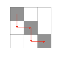
Figure 2: The Gurobi’s path optimization on $3\times 3$ bed with gray print region

VI Experimental Evaluation

In this section, we briefly describe our implementation and experimental evaluation. We implemented a Python tool box to automatically generate constraints corresponding to $\textit{Enc}(\textit{S},d)$ in the Gurobi input format, given a scenario S and a time bound $d$. Gurobi is an MILP solver, which returns the optimal assignment. We have implemented an algorithm to extract the optimal annotated plan from the optimal assignment.

We consider a diagonal pattern, that is, the print region corresponds to the diagonal cells in an $n\times n$ grid to evaluate our method. We experiment with varying grid sizes (increasing values of $n$), and with two different settings for temperature bounds. The results are presented in Table I and Table II. Our experiments have been conducted on 2.8 GHz Intel Core i7 Laptop. Dimensions represents the size of the grid, $d$ denotes the time bound, $m$ denotes cost of the returned path (length of the path until the last printed cell), the time taken to encode the constraints in seconds and the time taken by Gurobi to find the value of $m$ (and the optimal assignment).

TABLE I: Diagonal print pattern with $\textit{T}_{l}=0$ and $\textit{T}_{u}=200$

Dimensions	2$\times$ 2	3$\times$ 3	5$\times$ 5	7$\times$ 7
d	10	10	10	15
m	2	4	8	14
Encoding time	0.035	0.06	0.194	0.581
MILP solving time	0.065	0.12	0.848	10.306

First, we observe from Table I for the diagonal printing pattern with $\textit{T}_{l}=0$ and $\textit{T}_{u}=200$ that both the encoding time and the MILP solving time increase as we increase the size of the grid. However, MILP solving time, increases much faster than the encoding time, which points to the fact that MILP is an NP-complete problem. Also, we had a time-out of $1$ minute, and the procedure times out for $9\times 9$ grid. In all the cases, we obtained the shortest path to be the step plan along the diagonal as illustrated in Figure 2.

TABLE II: Diagonal print pattern with $\textit{T}_{l}=65$ and $\textit{T}_{u}=85$

Dimentions	2$\times$ 2	3$\times$ 3	5$\times$ 5	7$\times$ 7
d	10	10	10	15
m	6	7	9	NF
Encoding time	0.039	0.072	0.19	NF
MILP solving time	0.17	0.12	0.62	NF

Table II for the diagonal printing pattern with $\textit{T}_{l}=65$ and $\textit{T}_{u}=86$, we have a similar observation about the encoding and MILP solving time. However, with this reduced range for the temperature, we observe that the values of $m$ are relatively larger. In fact, when given a bound of $15$ for the $7\times 7$ grid, the procedure returned infeasible, indicating a potential plan that satisfies all the constraints would be longer. We observed that the path consisted sometime of repeated consecutive positioning of the nozzle at a particular cell. We conjecture that this is to satisfy the temperature constraints, and may corresponding to allow “cooling” of the cell temperatures.

VII Conclusion

In this paper, we addressed the problem of optimal path planning with spatio-temporal and thermal constraints, that arise naturally in the context of 3D printer tool path planning for superior structural properties. We considered a discrete version of the problem, and reduced the problem to MILP problem, which we solved using off-the-shelf solvers. Our experimental analysis demonstrated the feasibility of the approach. In the future, we will explore a continuous version of the problem, where we consider a PDE heat equation and generate continuous plans that specify velocity and acceleration of the print head.

References

- [1] S. M. LaValle, Planning Algorithms. Cambridge University Press, 2006.
- [2] J.-C. Latombe, Robot Motion Planning. Kluwer Academic Publishers, 1991.
- [3] V. Damodaran, A. Castellanos, M. Milostan, and P. Prabhakar, “Improving the mode-ii interlaminar fracture toughness of polymeric matrix composites through additive manufacturing,” Materials & Design, vol. 157, pp. 60 – 73, 2018.
- [4] E. Galceran and M. Carreras, “A survey on coverage path planning for robotics,” Robotics and Autonomous systems, 2013.
- [5] S. X. Yang and C. Luo, “A neural network approach to complete coverage path planning,” IEEE Transactions on Systems, Man, and Cybernetics, Part B (Cybernetics), 2004.
- [6] H. Choset, “Coverage for robotics–a survey of recent results,” Annals of mathematics and artificial intelligence, 2001.
- [7] A. Stentz, “Optimal and efficient path planning for partially-known environments,” in Robotics and Automation. Proceedings., IEEE International Conference on, 1994.
- [8] G. Yang and V. Kapila, “Optimal path planning for unmanned air vehicles with kinematic and tactical constraints,” in Decision and Control, 2002, Proceedings of the 41st IEEE Conference on, 2002.
- [9] M. Lepetič, G. Klančar, I. Škrjanc, D. Matko, and B. Potočnik, “Time optimal path planning considering acceleration limits,” Robotics and Autonomous Systems, 2003.
- [10] T. McGee, S. Spry, and K. Hedrick, “Optimal path planning in a constant wind with a bounded turning rate,” in AIAA Guidance, Navigation, and Control Conference and Exhibit, 2005.
- [11] T. G. McGee and J. K. Hedrick, “Optimal path planning with a kinematic airplane model,” Journal of guidance, control, and dynamics, 2007.
- [12] W. Wu, H. Chen, and P.-Y. Woo, “Time optimal path planning for a wheeled mobile robot,” Journal of Robotic Systems, 2000.
- [13] P. Bhattacharya and M. L. Gavrilova, “Voronoi diagram in optimal path planning,” in Voronoi Diagrams in Science and Engineering, 2007. ISVD’07. 4th International Symposium on, 2007.
- [14] S. L. Smith, J. Tuumova, C. Belta, and D. Rus, “Optimal path planning for surveillance with temporal-logic constraints,” The International Journal of Robotics Research, 2011.
- [15] R. Lal, A. Sharda, and P. Prabhakar, “Optimal multi-robot path planning for pesticide spraying in agricultural fields,” in 56th IEEE Annual Conference on Decision and Control, CDC 2017, Melbourne, Australia, December 12-15, 2017, 2017, pp. 5815–5820.
- [16] M. R. Dunlavey, “Efficient polygon-filling algorithms for raster displays,” ACM Transactions on Graphics (TOG), 1983.
- [17] S. C. Park and B. K. Choi, “Tool-path planning for direction-parallel area milling,” Computer-Aided Design, 2000.
- [18] R. Farouki, T. Koenig, K. Tarabanis, J. Korein, and J. Batchelder, “Path planning with offset curves for layered fabrication processes,” Journal of Manufacturing Systems, 1995.
- [19] H. Wang and J. A. Stori, “A metric-based approach to 2d tool-path optimization for high-speed machining,” in ASME 2002 International Mechanical Engineering Congress and Exposition, 2002.
- [20] P. Kulkarni, A. Marsan, and D. Dutta, “A review of process planning techniques in layered manufacturing,” Rapid prototyping journal, 2000.
- [21] P. K. Wah, K. G. Murty, A. Joneja, and L. C. Chiu, “Tool path optimization in layered manufacturing,” Iie Transactions, 2002.
- [22] G. Dreifus, K. Goodrick, S. Giles, M. Patel, R. M. Foster, C. Williams, J. Lindahl, B. Post, A. Roschli, L. Love, et al., “Path optimization along lattices in additive manufacturing using the chinese postman problem,” 3D Printing and Additive Manufacturing, 2017.
- [23] K.-Y. Fok, C.-T. Cheng, and K. T. Chi, “A refinement process for nozzle path planning in 3d printing,” in Circuits and Systems (ISCAS), 2017.
- [24] N. Ganganath, C.-T. Cheng, K.-Y. Fok, and K. T. Chi, “Trajectory planning for 3d printing: A revisit to traveling salesman problem,” in Control, Automation and Robotics (ICCAR), 2016.
- [25] K.-Y. Fok, C.-T. Cheng, K. T. Chi, and N. Ganganath, “A relaxation scheme for tsp-based 3d printing path optimizer,” in Cyber-Enabled Distributed Computing and Knowledge Discovery (CyberC), 2016 International Conference on, 2016.
- [26] K.-Y. Fok, N. Ganganath, C.-T. Cheng, and K. T. Chi, “A 3d printing path optimizer based on christofides algorithm,” in Consumer Electronics-Taiwan (ICCE-TW), 2016 IEEE International Conference on, 2016.
- [27] G. N. Frederickson, “Approximation algorithms for some postman problems,” Journal of the ACM (JACM), 1979.
- [28] P. Lechowicz, L. Koszalka, I. Pozniak-Koszalka, and A. Kasprzak, “Path optimization in 3d printer: Algorithms and experimentation system,” in Computational and Business Intelligence (ISCBI), 2016 4th International Symposium on, 2016.
- [29] L. Gurobi Optimization, “Gurobi optimizer reference manual,” 2018. [Online]. Available: http://www.gurobi.com
- [30] I. I. C. O. Studio, “CPLEX,” 2018. [Online]. Available: http://www.cplex.com