Plasmons in anisotropic Dirac systems

Abstract

We consider the plasmon excitations in anisotropic two-dimensional Dirac systems, be it either anisotropic graphene or surfaces of topological insulators. Generalizing the exact density-density response function one finds a plasmon dispersion that is anisotropic already at the lowest frequencies. Asymptotic expressions are obtained for the dispersion in this regime. We show that the plasmon properties of the complete material class of anisotropic Dirac systems are characterized by just two dimensionless material parameters. The strong anisotropy can be used to guide the plasmon modes, introducing new functionalities to the field of Dirac plasmonics.

I Introduction

Graphene and topological insulators (TI) are two-dimensional (2D) Dirac systems Geim07 ; Kane05 in the sense that they have a linear electron (and hole) dispersion and a Dirac point where the Fermi surface shrinks to zero. The peculiarities of relativistic electrons and the high Fermi velocity make them unique systems to study fundamental phenomena like spin-momentum locking and open many interesting applications in nano-electronics. Replacing the spin in TI by the pseudo-spin in graphene leads to a high formal analogy between both types of systems, be it that the number of Dirac cones that are present in the 2D Brioullin zone in one case is odd and in the other even. In the doped case, these Dirac systems allow for collective charge excitations – plasmons – that are different from both bulk and surface plasmons of ordinary metals. A pure 2D Dirac plasmon, like its 3D counterpart, has no direct coupling to light due to the momentum mismatch. However, such a coupling can be created by proper surface modification that break translation symmetry, for instance by grating or nano-structuration. This allows for interesting applications such as terahertz photodetectors, motivating the field of graphene plasmonics, or more in general, Dirac plasmonics.kochnl11 ; Grigorenko12 ; diornn13 ; gaap14

Here we concentrate on systems having an anisotropic Dirac cone in particular with a high factor of anisotropy $A=v_{x}/v_{y}$ between two extremal Fermi velocities in the two perpendicular directions $x$ and $y$. A large factor of $A=18$ was for instance predicted for the topological surface states of the 3D TI HgS, Virot11 but other TI’s can have large anisotropy factors as well. Zhang11 Experimentally anisotropic Dirac cones were detected recently by angle resolved photoemission in for instance Ru₂Sn₃,gievsr14 CaMnBi₂,fewasr14 BaMnBi₂, and BaZnBi₂.Ryu18 In graphene the Dirac cone warping produces some anisotropy in the dispersion of the 2D and acoustic plasmons.himiepl09 ; gayussc11 ; denoprb13 ; pisinjp14 External strain can cause spatial anisotropy in graphene, but the expected changes in the plasmon anisotropy are rather small.Choi10

Quite a considerable amount of theoretical work had been devoted to tilted Dirac cones which can be found in $\alpha$-(BEDT-TTF)₂I₃ (BEDT-TTF=bis(ethylene-dithio)tetrathiafuva) under pressure,Tajima06 in some other organic quasi-two-dimensional materials as well as in orthorombic borophene.Feng17 The analytical result for the imaginary part of the density-density response has been given in Ref. Nishine10, and for the real part in Ref.  Sadhukhan17, . There, also a slight anisotropy was included. Plasmons of a tilted cone in a magnetic field were analyzed in Ref. Sari14, . However, the analytical formula of Ref. Sadhukhan17, was criticized in Ref. Jalali18, and we will clarify that point here for any possible anisotropic Dirac system. We will not consider the effect of tilting, but rather only spatial anisotropy that lowers in-plane rotation symmetry which is the usual case for anisotropic TI’s and for this situation will provide analytical expressions for the full plasmon dispersion and certain limiting cases. We are going to derive handy analytical formulas for the anisotropic plasmon dispersion of a general anisotropic Dirac system being characterized by just 2 dimensionless material parameters.

II Hamiltonian and charge response

We are considering electrons confined to two dimensions with Coulomb interactions. The Hamiltonian of an anisotropic Dirac system is given by

$$H=\sum_{\bf k}\varepsilon_{\bf k}c_{{\bf k}\uparrow}^{\dagger}c_{{\bf k}\downarrow}+\varepsilon_{\bf k}^{*}c_{{\bf k}\downarrow}^{\dagger}c_{{\bf k}\uparrow}\;,$$ (1)

where $c^{\dagger}$/$c$ represent fermion creation/annihilation operators, $\bf k$ the 2D wavevector and the energy is given in terms of the velocities $v_{x}$/$v_{y}$ in $x$/$y$ direction as

$$\varepsilon_{\bf k}=v_{y}k_{y}+{\rm i}v_{x}k_{x}=\lvert\varepsilon_{\bf k}\rvert\exp({\rm i}\Phi_{\bf k})\;.$$ (2)

The Hamiltonian describes anisotropic topological insulators or graphene if one replaces spin by pseudo spin and adds valley and spin degeneracies. The plasmon dispersion can then be obtained by calculating the dielectric function in random phase approximation (RPA). The dielectric function at 2D wave vector ${\bf q}$ and energy transfer $\omega$ is related with the charge susceptibility (or density-density response function)

$$\chi(\bf{q},\omega)=\langle\langle\rho_{\bf q};\rho_{\bf-q}\rangle\rangle$$ (3)

with

$$\rho_{\bf q}=\sum_{{\bf k}\sigma}c_{{\bf k}\sigma}^{\dagger}c_{{\bf k+q}\sigma}$$

being expressed via a retarded Green’s function. In RPA we obtain

$$\chi({\bf q},\omega)=\frac{\chi_{0}({\bf q},\omega)}{1-V({\bf q})\chi_{0}({\bf q},\omega)}\;,$$ (4)

where $\chi_{0}$ is the electron-hole bubble (in graphical representation) and $V({\bf q})=e^{2}/(2\lvert{\bf q}\rvert\varepsilon_{0}\varepsilon_{rel})$ is the Coulomb interaction in the 2D system. Following the calculation for the isotropic case Wunsch06 ; Hwang07 ; Principi09 we generalize it to the anisotropic situation. By diagonalizing (1) one finds two energy branches $\pm\lvert\varepsilon_{\bf k}\rvert=\lambda\lvert\varepsilon_{\bf k}\rvert$. The unitary transformation

$$\tilde{c}_{{\bf k}\pm}=(c_{{\bf k}\uparrow}\exp(-{\rm i}\phi_{\bf k}/2)\pm c_{{\bf k}\downarrow}\exp({\rm i}\phi_{\bf k}/2))/\sqrt{2}$$

diagonalizes the Hamiltonian (1) and gives the zero-order susceptibility as:

$$\chi_{0}({\bf q},\omega)=\sum_{\lambda\lambda^{\prime}}\chi_{0}^{\lambda\lambda^{\prime}}=g\sum_{{\bf k}\lambda\lambda^{\prime}}\frac{F^{\lambda\lambda^{\prime}}(n_{{\bf k}\lambda}-n_{{\bf k+q}\lambda^{\prime}})}{\omega+{\rm i}0^{+}+\lambda\lvert\varepsilon_{\bf k}\rvert-\lambda^{\prime}\lvert\varepsilon_{\bf k+q}\rvert}\;,$$

where $g$ is an eventual degeneracy ($g=4$ in graphene due to spin and valley degeneracy). Also, $\{\lambda,\lambda^{\prime}\}=\pm 1$ denote the two branches of the dispersion and $n_{{\bf k}\lambda}$ is in general the Fermi function $n_{{\bf k}\lambda}=f(\lambda\lvert\varepsilon_{\bf k}\rvert-\varepsilon_{F})$ of the $\lambda$ branch but we restrict ourselves here to zero temperature and $\varepsilon_{F}$ is the Fermi energy. The form factor is

$$F^{\lambda\lambda^{\prime}}=(1+\lambda\lambda^{\prime}\cos(\Phi_{\bf k+q}-\Phi_{\bf k}))/2\;.$$

We consider now a doped situation with a Fermi energy $\varepsilon_{F}$ lying in the positive branch $\lambda=+1$. Since the negative branch is completely filled, $\chi_{0}^{--}$ is zero. We are interested in the real part of $\chi_{0}$ to determine the plasmon dispersion via the zero of the denominator of (4). As in the isotropic case, the plasmon dispersion is dominated by $\chi_{0}^{++}$ which can be expressed as:

$$\chi_{0}^{++}=g\iint_{\varepsilon_{\bf k}<\varepsilon_{F}}\frac{\rm dk_{x}\rm dk_{y}}{4\pi^{2}}\frac{F^{++}(\lvert\varepsilon_{\bf k+q}\rvert-\lvert\varepsilon_{\bf k}\rvert)}{\omega^{2}-(\lvert\varepsilon_{\bf k+q}\rvert-\lvert\varepsilon_{\bf k}\rvert)^{2}}\;.$$ (5)

After introducing vectors ${\bf K}$ and ${\bf Q}$ with $K_{i}=k_{i}v_{i}/v$, $Q_{i}=q_{i}v_{i}/v$ ($i=\{x,y\}$) and $v^{2}=v_{x}v_{y}$ we can write $\lvert\varepsilon_{\bf k}\rvert=v\lvert{\bf K}\rvert$ and cast integral (5) into the same form as for the isotropic case

$$\chi_{0}^{++}=g\iint_{\lvert{\bf K}\rvert<\frac{\varepsilon_{F}}{v}}\frac{\rm dK_{x}\rm dK_{y}}{4\pi^{2}}\frac{F^{++}v(\lvert{\bf K+Q}\rvert-\lvert{\bf K}\rvert)}{\omega^{2}-v^{2}(\lvert{\bf K+Q}\rvert-{\bf K}\rvert)^{2}}\;.$$

We also see that $\Phi_{{\bf k+q}}-\Phi_{{\bf k}}$ equals the angle between ${\bf K+Q}$ and ${\bf K}$. Therefore, we can use for $\chi_{0}^{++}$ at wave vector ${\bf q}$ in the anisotropic case the expression for the isotropic case $\chi_{0}^{++,{\rm iso}}$ at wave vector ${\bf Q}$ which is also true for the other contributions $\chi_{0}^{+-}$ and $\chi_{0}^{-+}$. We find finally

$$\chi_{0}({\bf q},\omega)=\chi_{0}^{{\rm iso}}({\bf Q},\omega)\;,$$ (6)

where we have to use the Fermi velocity $v=\sqrt{v_{x}v_{y}}$ in $\chi_{0}^{{\rm iso}}$. The exact expression of $\chi_{0}^{{\rm iso}}$ in the isotropic case is well known, Wunsch06 ; Hwang07 but it now depends on $Q=\lvert{\bf Q}\rvert$ instead of $q=\lvert{\bf q}\rvert$. The dependence on the angle $\alpha$ of the plasmon propagation, where $q_{x}=q\cos\alpha$ and $q_{y}=q\sin\alpha$ can be cast into a directional factor $D$:

$$Q=qD\quad,\quad D=\sqrt{A\cos^{2}\alpha+\frac{\sin^{2}\alpha}{A}}\;.$$ (7)

Using the known expression for $\chi_{0}^{{\rm iso}}$, we find the exact expression for the density-density response function in the anisotropic case. It can be expressed like

$$\chi_{0}({\bf q},\omega)=Cg(\kappa,\nu)\quad,\quad C=\frac{g\varepsilon_{F}}{2\pi v^{2}\hbar^{2}}\;,$$ (8)

in dependence on the dimensionless parameters

$$\nu=\frac{\hbar\omega}{\varepsilon_{F}}\quad,\quad\kappa=\frac{q}{q_{F}}D\;,$$ (9)

where we introduce $\hbar$ from now on with $q_{F}$ being an averaged Fermi wave vector defined by $\varepsilon_{F}=\hbar vq_{F}$, and where

$$g(\kappa,\nu)=-1+f\left(G_{+}\left(\frac{2+\nu}{\kappa}\right)-G_{+}\left(\frac{2-\nu}{\kappa}\right)\right)$$

and

$$f=\frac{\kappa^{2}}{8\sqrt{\nu^{2}-\kappa^{2}}}\,,\,G_{+}(x)=x\sqrt{x^{2}-1}-\ln{(x+\sqrt{x^{2}+1})}\;.$$

This expression for the real part outside the continuum of electron-hole excitations whose border is given by $\nu=\kappa$ and $\nu=2-\kappa$ and where the imaginary part of $\chi_{0}$ is zero derives from the complete expression given in Refs. Wunsch06, ; Hwang07, . The analytical expression (8) can also be obtained from the tilted case Sadhukhan17 ; Jalali18 by putting the tilt angle to zero in which case the difference between Refs. Sadhukhan17, and Jalali18, disappears.

We are interested in the plasmon dispersion in the hydrodynamic limit $\omega\to 0$ and $q\to 0$ where we can use the leading-order expression Raghu10 :

$$g(\kappa,\nu)=\frac{\nu^{2}}{\sqrt{\nu^{2}-\kappa^{2}}}-1\;.$$ (10)

For $\nu\gg\kappa$ that simplifies to

$$g(\kappa,\nu)=\frac{\kappa^{2}}{2\nu^{2}}\;.$$ (11)

To illustrate the different approximations we present them in Fig. 1 together with the exact expression for $\nu=0.6$. At small $q$ all three expressions coincide, but $\chi_{0}$ diverges if $\kappa=Dq/q_{F}$ approaches the continuum of particle-hole excitations $\kappa=\nu$ which is not the case in the parabolic approximation in Eq.  (11).

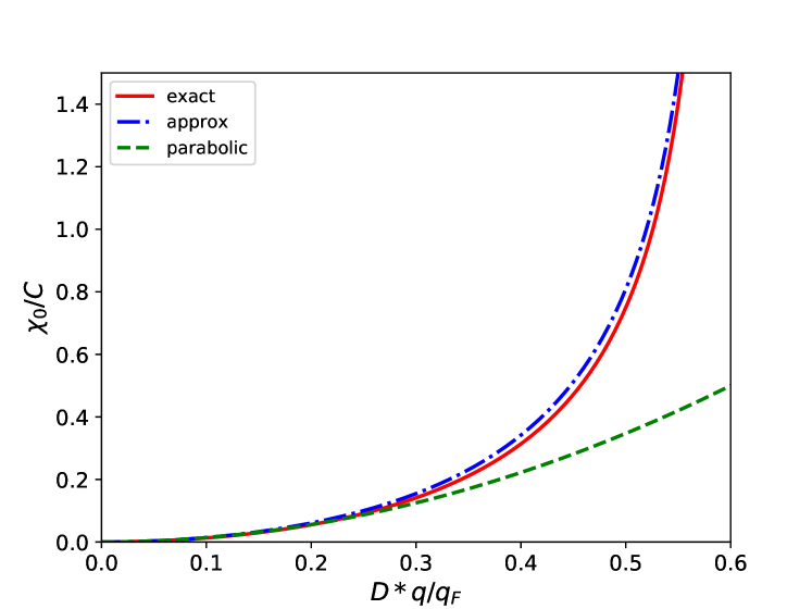
Figure 1: Real part of the zero-order density-density response function $\chi_{0}/C$ for $\nu=\hbar\omega/\varepsilon_{F}=0.6$. Compared are the exact expression (red, full line) with the approximative one (Eq. (10), blue dash-dotted line) and the parabolic approximation (Eq. (11), green dashed line).

III Plasmon

The plasmon dispersion is determined by solving $V({\bf q})\chi_{0}({\bf q},\omega)=1$ which is in dimensionless form

$$\frac{q}{q_{F}}=2\beta g(\kappa,\nu)\;,$$ (12)

where we introduce the dimensionless material parameter

$$\beta=\frac{ge^{2}}{8\pi\varepsilon_{0}\varepsilon_{rel}\hbar v}\;.$$ (13)

In the parabolic approximation for small $q$ and $\omega$ the plasmon dispersion can be explicitly given,

$$\frac{\hbar\omega}{\varepsilon_{F}}=\sqrt{\beta}\sqrt{\frac{q}{q_{F}}}D\;,$$ (14)

and is especially simple. The square-root dispersion is of course characteristic to 2D systems.

Any anisotropic Dirac system is characterized by the degeneracy $g$, the Fermi velocity $v$, the anisotropy $A=v_{x}/v_{y}$, the relative dielectric constant $\varepsilon_{rel}$, and the Fermi energy $\varepsilon_{F}$ closely related with the filling of the Dirac cone. The plasmon dispersion which is given by the solution of (12) is valid for any anisotropic Dirac system and characterized by just two material parameters $\beta$ and $A$. At the same time, without tilting, the analytical result (12) is rather simple.

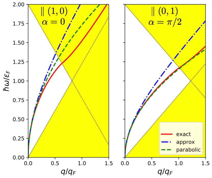
Figure 2: Plasmon dispersion for material parameters $\beta=2.0$ and $A=1.5$ for the two extremal plasmon propagation directions $\alpha=0$ (left) and $\alpha=\pi/2$ (right) using the exact expression or the two approximate ones (see Fig. 1) together with the corresponding boundaries of the continuum of electron-hole excitations (yellow) shown by dotted lines.

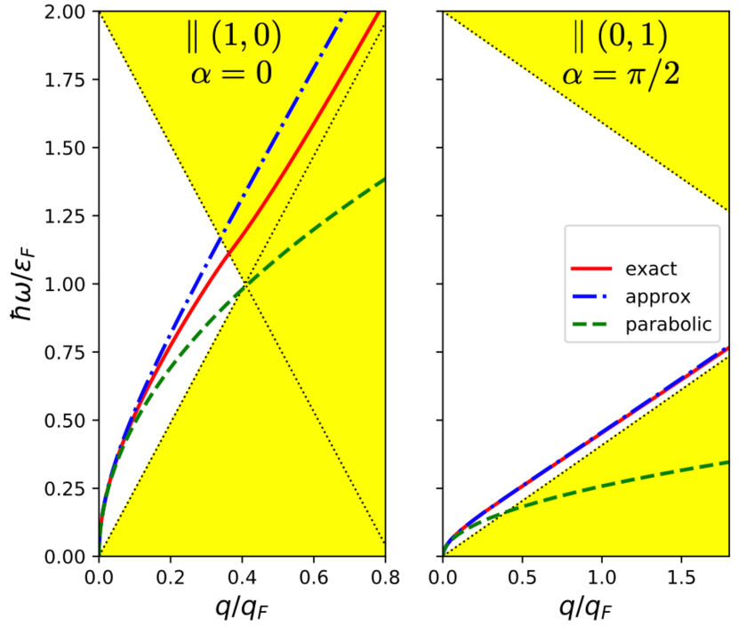
Figure 3: Plasmon dispersion for material parameters $\beta=0.4$ and $A=6.0$ for the two extremal plasmon propagation directions $\alpha=0$ (left) and $\alpha=\pi/2$ (right) using the exact expression or the two approximate ones (see Figs. 1 and 2). The continuum of electron-hole excitations is indicated in yellow.

The exact plasmon dispersion together with that one resulting from the two approximations (10) and (11) is shown in Figs. 2 and 3 for two different sets of material parameters. In all cases, we show the two extremal directions $\alpha=0$ and $\alpha=\pi/2$. The behavior is different for materials with $\beta$ larger than one and having a relatively small anisotropy (represented in Fig. 2 for $\beta=2.0$ and $A=1.5$) from that one for $\beta$ being considerably smaller than one and having a large anisotropy (Fig. 3 for $\beta=0.4$ and $A=6.0$). In Fig. 2 both approximations represent relatively well the exact plasmon dispersion. The square-root dispersion never crosses the line $\nu=\kappa$ and enters into the continuum of electron-hole excitations where it gets a final life-time by crossing the upper line $\nu=2-\kappa$. That is different in Fig. 3. There the square-root dispersion crosses the line $\nu=\kappa$ which is especially visible for $\alpha=\pi/2$ in the right hand part of the figure. Just relying on the parabolic approximation would imply that the plasmon becomes damped above a critical value $\nu_{c}=\beta/\sqrt{A}$ which was incorrectly inferred in Ref. Raghu10, for Bi₂Se₃. In effect, due to the divergence of $\chi_{0}$ at $\nu=\kappa$, the exact plasmon dispersion can never cross the line $\nu=\kappa$ such that the plasmon remains undamped up to a critical $\nu_{c}$ of order one. Lines of constant plasmon energy are shown in Fig. 4 for $\beta=2.0$ and $A=2.5$. Clearly, they deviate strongly from simple ellipses which are expected for a tilted Dirac cone Jalali18 and show a remarkable anisotropy which increases at small plasmon energies.

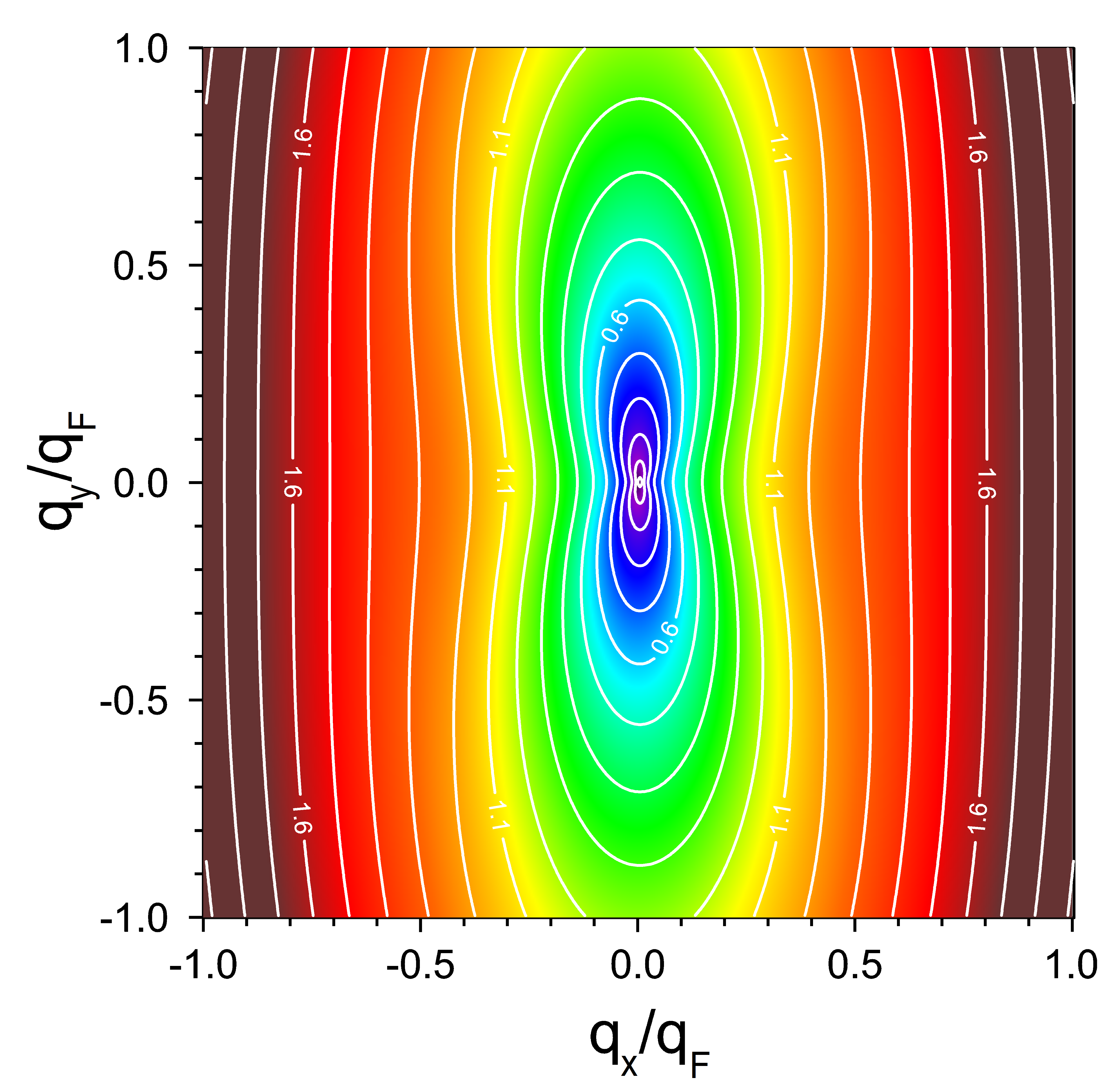
Figure 4: Contour plot of the anisotropic plasmon dispersion with lines of constant plasmon energy in the $q_{x}$-$q_{y}$ plane for material parameters $\beta=2.0$ and $A=2.5$.

IV Materials

The material parameter $\beta$ can vary quite considerably in different Dirac systems. For graphene with $g=4$, $\varepsilon_{rel}=2.4$, and $v=9\times 10^{5}ms^{-1}$, one finds $\beta=2.08$, exceeding $\beta=1$ considerably.

For Bi₂Se₃ a bulk dielectric constant perpendicular to the $c$-axis of $\varepsilon_{rel}\approx 27$ was obtained in the first-principles calculations.nehaprb13 Experimentally determined $\varepsilon_{rel}\approx 29$ was obtained using single crystals.Richter77 ; Stordeur92 Employing the latter value together with $v=5\times 10^{5}ms^{-1}$ and $g=1$ leads to $\beta=0.10$, which compares well with the simulation of the measured plasmon dispersion in Ref. Politano15, .

Turning to anisotropic Dirac systems we have to distinguish two different cases, systems like HgS or Ag₂Te with a preferred direction of plasmon propagation, or materials of the BaMnBi₂ class which preserve a fourfold rotation symmetry axis at the surface despite the strong anisotropy of the Dirac cones. Our theory directly applies to the first class of systems. The anisotropy factor was predicted to be 18 (HgS)Virot11 or about 10 (Ag₂Te)Zhang11 . The $\beta$ parameter is more difficult to estimate due to the uncertain knowledge about $\varepsilon_{rel}$. By comparison with Bi₂Se₃ the $\beta$ parameter can be assumed to be smaller or close to 1. So one expects a scenario close to that reported in Fig. 3, with an even higher anisotropy factor $A$.

For the other class of anisotropic Dirac cones with conserved 4 fold rotation symmetry, there are all together 4 anisotropic Dirac cones being pairwise perpendicular to each other. Therefore, one obtains four contributions to $\chi_{0}$:

$$\chi_{0}=\frac{g\varepsilon_{F}}{4\pi}\left(\frac{{{\bf Q}_{1}}^{2}}{\omega^{2}}+\frac{{{\bf Q}_{2}}^{2}}{\omega^{2}}\right)\;,$$ (15)

where the preferred direction of one cone ${{\bf Q}_{1}}^{2}=q^{2}(A\cos^{2}\alpha+\sin^{2}\alpha/A)$ is perpendicular to that one of the other cone ${{\bf Q}_{2}}^{2}=q^{2}(A\sin^{2}\alpha+\cos^{2}\alpha/A)$ and $g=2$. We see that the anisotropy disappears in the leading order and remains only in higher orders. The anisotropy is expected to be much smaller than in the other class of anisotropic TI’s and to appear only for larger values of $q$ as is quite usual in many realistic materials.

V Discussion and conclusions

We have shown how the well-known square-root dispersion for 2D Dirac plasmons can be generalized to the anisotropic case. Interestingly, the entire material class of anisotropic Dirac systems can be described by just two material parameters $\beta$ and $A$. For materials with small values of $\beta$ the square-root dispersion applies only for very small frequencies and has to be replaced by a more exact one close to the continuum of electron-hole excitations. Materials with high anisotropy factor $A$ show strongly anisotropic plasmon excitations in the entire energy range up to very small frequencies. Controlling either of the material parameters opens the pathway to engineer and customize 2D Dirac systems for plasmonics. In particular, for high anisotropies, plasmon wave guides may be constructed.maaln18 ; mashim20 It should be mentioned, that anisotropic low-energy plasmons can also be realized in other 2D systems with a non-linear band dispersion like phosphorene,loroprl14 ; lagujap15 ; ghthprb17 ; savaprb17 ; lemaap18 ; wazhaom20 borophene,hushjacs17 ; lihuprl20 ; delioe20 and MoS₂.toasjpcm17 However, the amount of anisotropy is not so pronounced there as we predict here.

Verifying the predicted anisotropy of the plasmon dispersion requires measurements at the surface of anisotropic TI’s. One interesting candidate system is Ag₂Te for which the anisotropic Dirac cone was experimentally verified. A useful technique to measure the plasmon dispersion at the surface of a TI is electron energy loss spectroscopy (EELS) in reflection geometry. Also optical measurements are possible that require periodic structure modifications, for instance surface grating.

Acknowledgements - R.H. thanks M. Knupfer, S.-L. Drechsler, and M. Richter for very helpful discussions. V.M.S. acknowledges financial support from the Spanish Ministry Science and Innovation (Grant No. PID2019-105488GB-I00). J.v.d.B. acknowledges financial support from the German Research Foundation (Deutsche Forschungsgemeinschaft, DFG) via SFB1143 Project No. A5 and under Germanys Excellence Strategy through the Würzburg-Dresden Cluster of Excellence on Complexity and Topology in Quantum Matter ct.qmat (EXC 2147, Project No. 390858490).

References

- (1) A. K. Geim and K. S. Novoselov, Nature Mater. 6, 183 (2007).
- (2) C. L. Kane and E. J. Mele, Phys. Rev. Lett. 95, 146802 (2005).
- (3) A.N. Grigorenko, M. Polini, and K. S. Novoselov, Nature Photon. 6, 749 (2012).
- (4) F. H. L. Koppens, D. E. Chang, and F. J. Garcia de Abajo, Nano Lett. 11, 3370 (2011).
- (5) P. Di Pietro, M. Ortolani, O. Limaj, A. Di Gaspare, V. Giliberti, F. Giorgianni, M. Brahlek, N. Bansal, N. Koirala, S. Oh, P. Calvani, and S. Lupi, Nat. Nanotechnol. 8, 556 (2013).
- (6) F. J. Garcia de Abajo, ACS Photonics 1, 135 (2014).
- (7) F. Virot, R. Hayn, M. Richter, and J. van den Brink, Phys. Rev. Lett. 106, 236806 (2011).
- (8) W. Zhang, R. Yu, W. Feng, Y. Yao, H. Weng, X. Dai, and Z. Fang, Phys. Rev. Lett. 106, 156808 (2011).
- (9) Q. D. Gibson, D. Evtushinsky, A. N. Yaresko, V. B. Zabolotnyy, M. N. Ali, M. K. Fuccillo, J. van den Brink, B. Büchner, R. J. Cava, and S. V. Borisenko, Sci. Rep. 4, 5168 (2014).
- (10) Y. Feng, Z. J. Wang, C. Y. Chen, Y. G. Shi, Z. J. Xie, H. A. Yi, A. J. Liang, S. L. He, J. F. He, Y. Y. Peng, X. Liu, Y. Liu, L. Zhao, G. D. Liu, X. O. Dong, J. Zhang, C. T. Chen, Z. A. Xu, X. Dai, Z. Fang, and X. J. Zhou, Sci. Rep. 4, 5385 (2014).
- (11) H.Ryu, S.Y. Park, L.Li, W. Ren, J.B. Neaton, C. Petrovic, C. Hwang, and S.-K. Mo, Sci. Rep. 8, 15322 (2018).
- (12) A. Hill, S. A. Mikhailov, and K. Ziegler, EPL 87, 27005 (2009).
- (13) Y. Gao and Z. Yuan, Solid State Commun. 151, 1009 (2011).
- (14) V. Despoja, D. Novko, K. Dekanić, M. Šunjić, and L. Marušić, Phys. Rev. B 87, 075447 (2013).
- (15) M. Pisarra, A. Sindona, P. Riccardi, V. M. Silkin, and J. M. Pitarke, New J. Phys. 16, 083003 (2014).
- (16) S.-M. Choi, S.-H. Jhi, and Y.-W. Son, Phys. Rev. B 81, 081407 (2010).
- (17) N. Tajima, S. Sugawara, M. Tamura, Y. Nishio, and K. Kajita, J. Phys. Soc. Jpn. 75, 051010 (2006).
- (18) B. Feng, O. Sugino, R.-Y. Liu, J. Zhang, R. Yukawa, M. Kawamura, T. Iimori, H. Kim, Y. Hasegawa, H. Li, L. Chen, K. Wu, H. Kumigashira, F. Komori, T.-C. Chiang, S. Meng, and I. Matsuda, Phys. Rev. Lett. 118, 096401 (2017).
- (19) T. Nishine, A. Kobayashi, and Y. Suzumura, J. Phys. Soc. Jpn. 79, 114715 (2010).
- (20) K. Sadhukhan and A. Agarwal, Phys. Rev. B 96, 035410 (2017).
- (21) J. Sári, C. Töke, and M.O. Goerbig, Phys. Rev. B 90, 155446 (2014).
- (22) Z. Jalali-Mola and S. A. Jafari, Phys. Rev. B 98, 195415 (2018).
- (23) B. Wunsch, T. Stauber, F. Sols, and F. Guinea, New J. Phys. 8, 318 (2006).
- (24) E. H. Hwang and S. Das Sarma, Phys. Rev. B 75, 205418 (2007).
- (25) A. Principi, M. Polini, and G. Vignale, Phys. Rev. B 80, 075418 (2009).
- (26) S. Raghu, S. B. Chung, X.-L. Qi, and S.-C. Zhang, Phys. Rev. Lett. 104, 116401 (2010).
- (27) I. A. Nechaev, R. C. Hatch, M. Bianchi, D. Guan, C. Friedrich, I. Aguilera, J. L. Mi, B. B. Iversen, S. Blügel, Ph. Hofmann, and E. V. Chulkov, Phys. Rev. B 87, 121111 (2013).
- (28) W. Richter, H. Köhler, and C. R. Becker, Phys. Stat. Sol. (b) 84, 619 (1977).
- (29) M. Stordeur, K. K. Ketavonc, A. Priemuth, H. Sobotta, and V. Riede, Phys. Stat. Sol. (b) 169, 505 (1992).
- (30) A. Politano, V. M. Silkin, I. A. Nechaev, M. S. Vitiello, L. Viti, Z. S. Aliev, M. B. Babanly, G. Chiarello, P. M. Echenique, and E. V. Chulkov, Phys. Rev. Lett. 115, 216802 (2015).
- (31) W.-L. Ma, P. Alonso-González, S.-J. Li, A. Y. Nikitin, J. Yuan, J. Martín-Sánchez, J. Taboada-Gutiérrez, I. Amenabar, P.-N. Li, S. Vélez, C. Tollan, Z.-G. Dai, Y.-P. Zhang, S. Sriram, K. Kalantar-Zadeh, S.-T. Lee, R. Hillenbrand, and Q.-L. Bao, Nature 562, 557 (2018).
- (32) W.-L. Ma, B. Shabbir, Q.-D. Ou, Y.-M. Dong, H.-Y. Chen, P.-N. Li, X.-L. Zhang, Y.-R. Lu, and Q.-L. Bao, InfoMat. 2, 777 (2020).
- (33) T. Low, R. Roldán, H. Wang, F. Xia, P. Avouris, L. M. Moreno, and F. Guinea, Phys. Rev. Lett. 113, 106802 (2014).
- (34) R.-T. Lam and J. Guo, J. Appl. Phys. 117, 113105 (2015).
- (35) B. Ghosh, P. Kumar, A. Thakur, Y. S. Chauhan, S. Bhowmick, and A. Agarwal, Phys. Rev. B 96, 035422 (2017).
- (36) S. Saberi-Pouya, T. Vazifehshenas, T. Salavati-fard, and M. Farmanbar, Phys. Rev. B 96, 115402 (2017).
- (37) I.-H. Lee, L. Martin-Moreno, D. A. Mohr, K. Khaliji, T. Low, and S.-H. Oh, ACS Photonics 5, 2208 (2018).
- (38) C. Wang, G. W. Zhang, S. Y. Huang, Y. G. Xie, and H. Yan, Adv. Opt. Mater. 8, 1900996 (2020).
- (39) C. Lian, S.-Q. Hu, J. Zhang, C. Cheng, Z. Yuan, S. Gao, and S. Meng, Phys. Rev. Lett. 125, 116802 (2020).
- (40) S. A. Dereshgi, Z. Z. Liu, and K. Aydin, Opt. Exp. 28, 16725 (2020).
- (41) Y. Huang, S. N. Shikodkar, and B. I. Yakobson, J. Amer. Chem. Soc. 139, 17181 (2017).
- (42) Z. Torbatian and R. Asgari, J. Phys.: Condens. Matter 29, 465701 (2017).