Improved Approximation Algorithms for Tverberg Partitions

Abstract

Tverberg’s theorem states that a set of $n$ points in $\mathbb{R}^{d}$ can be partitioned into $\left\lceil{n/(d+1)}\right\rceil$ sets whose convex hulls all intersect. A point in the intersection (aka Tverberg point) is a centerpoint, or high-dimensional median, of the input point set. While randomized algorithms exist to find centerpoints with some failure probability, a partition for a Tverberg point provides a certificate of its correctness.

Unfortunately, known algorithms for computing exact Tverberg points take $n^{O(d^{2})}$ time. We provide several new approximation algorithms for this problem, which improve running time or approximation quality over previous work. In particular, we provide the first strongly polynomial (in both $n$ and $d$) approximation algorithm for finding a Tverberg point.

1 Introduction

Given a set $P$ of $n$ points in the plane and a query point $q$, classification problems ask whether $q$ belongs to the same class as $P$. Some algorithms use the convex hull $\mathcal{CH}\left({P}\right)$ as a decision boundary for classifying $q$. However, in realistic datasets, $P$ may be noisy and contain outliers, and even one faraway point can dramatically enlarge the hull of $P$. Thus, we would like to measure how deeply $q$ lies within $P$ in way that is more robust against noise.

In this paper, we investigate the notion of Tverberg depth. However, there are many related measures of depth in the literature, including:

1. Tukey depth. The Tukey depth of $q$ is the minimum number of points that must be removed before $q$ becomes a vertex of the convex hull. Computing the depth is equivalent to computing the closed halfspace that contains $q$ and the smallest number of points of $P$, and this takes $O(n\log n)$ time in the plane [Cha04].

2. Centerpoint. In $\mathbb{R}^{d}$, a point with Tukey depth $n\alpha$ is an $\alpha$-centerpoint. There is always a $1/(d+1)$-centerpoint, known simply as the centerpoint, which can be computed exactly in $O(n^{d-1})$ time [JM94, Cha04]. It can be approximated using the centerpoint of a sample [CEM+96], but getting a polynomial-time (in both $n$ and $d$) approximation algorithm proved challenging. Clarkson et al. [CEM+96] provided an algorithm that computes a $1/4d^{2}$-centerpoint in roughly $O(d^{9})$ time. Miller and Sheehy [MS10] derandomized it to find a (roughly) $1/2d^{2}$-centerpoint in $n^{O(\log d)}$ time. More recently, Har-Peled and Mitchell [HJ19] improved the running time to compute a (roughly) $1/d^{2}$-centerpoint in (roughly) $O(d^{7})$ time.

3. Onion depth. Imagine peeling away the vertices of the current convex hull and removing them from $P$. The onion depth is the number of layers which must be removed before the point $q$ is exposed. The convex layers of points in the plane can be computed in $O(n\log n)$ time by an algorithm of Chazelle [Cha85]. The structure of convex layers is well-understood for random points [Dal04] and grid points [HL13].

4. Uncertainty. Another model considers uncertainty about the locations of the points. Suppose that each point of $P$ has a certain probability of existing, or alternatively, its location is given via a distribution. The depth of query point $q$ is the probability that $q$ is in the convex hull once $P$ has been sampled. Under certain assumptions, this probability can be computed exactly in $O(n\log n)$ time [AHS+17]. Unfortunately, the computed value might be very close to zero or one, and therefore tricky to interpret.

5. Simplicial depth. The simplicial depth of $q$ is the number of simplices induced by $P$ containing it. This number can be approximated quickly after some preprocessing [ASS15]. However, it can be quite large for a point which is intuitively shallow.

Tverberg depth.

Given a set $P$ of $n$ points in $\mathbb{R}^{d}$, a Tverberg partition is a partition of $P$ into $k$ disjoint sets $P_{1},\ldots,P_{k}$ such that $\bigcap_{i}\mathcal{CH}\left({P_{i}}\right)$ is not empty. A point in this intersection is a Tverberg point. Tverberg’s theorem states that $P$ has a Tverberg partition into $\left\lceil{n/(d+1)}\right\rceil$ sets. In particular, the Tverberg depth (T-depth) of a point $q$ is the maximum size $k$ of a Tverberg partition such that $q\in\bigcap_{i=1}^{k}\mathcal{CH}\left({P_{i}}\right)$.

By definition, points of T-depth $n/(d+1)$ are centerpoints for $P$. In the plane, Reay [Rea79] showed that if a point has Tukey depth $k\leq\left|{P}\right|/3$, then the T-depth of $q$ is $k$. This property is already false in three dimensions [Avi93]. The two-dimensional case was handled by Birch [Bir59], who proved that any set of $n$ points in the plane can be partitioned into $n/3$ triples whose induced triangles have a common intersection point.

Computing a Tverberg point.

For work on computing approximate Tverberg points, see [MS10, MW13, RS16, CM20] and the references therein. Currently, no polynomial-time (in both $n$ and $d$) approximation algorithm is known for computing Tverberg points. This search problem is believed to be quite hard, see [MMSS17].

Algorithms for computing an exact Tverberg point of T-depth $n/(d+1)$ implement the construction implied by the original proof. The runtime of such an algorithm is $d^{O(d^{2})}n^{d(d+1)+1},$ see Section 2.2. As previously mentioned, the exception is in two dimensions, where the algorithm of Birch [Bir59] runs in $O(n\log n)$ time. But even in three dimensions, we are unaware of an algorithm faster than $O(n^{13})$.

Convex combinations and Carathéodory’s theorem.

The challenge in finding a Tverberg point is that we have few subroutines at our disposal with runtimes polynomial in $d$. Consider the most basic task – given a set $P$ of $n$ points and a query point $q$, decide if $q$ lies inside $\mathcal{CH}\left({P}\right)$, and if so, compute the convex combination of $q$ in term of the points of $P$. This problem can be reduced to linear programming. Currently, the fastest strongly polynomial LP algorithms run in super-polynomial time $2^{O(\sqrt{d\log d})}+O(d^{2}n)$ [Cla95, MSW96], where $d$ is the number of variables and $n$ is the number of constraints. However, any given convex combination of $P$ representing $q$ can be sparsified in polynomial time into a convex combination using only $d+1$ points of $P$. Lemma 3.9 describes this algorithmic version of Carathéodory’s theorem.

Radon partitions in polynomial time.

Finding points of T-depth $2$ is relatively easy. Any set of $d+2$ points in $\mathbb{R}^{d}$ can be partitioned into two disjoint sets whose convex hulls intersect, and a point in the intersection is a Radon point. Radon points can be computed in $O(d^{3})$ time by solving a linear system with $d+2$ variables. Almost all the algorithms for finding Tverberg points mentioned above amplify the algorithm for finding Radon points.

Depth	Running time	Ref / Comment
$n/(d+1)$	$d^{O(d^{2})}n^{d(d+1)+1}\Bigr{.}$	Tverberg theorem
$d=2:\,n/3$	$O(n\log n)$	[Bir59]: Theorem 2.8
$\displaystyle\frac{n}{2(d+1)^{2}}\Bigr{.}$	$n^{O(\log d)}$	Miller and Sheehy [MS10]
$\displaystyle\frac{n}{4(d+1)^{3}}\Bigr{.}$	$d^{O(\log d)}n$	Mulzer and Werner [MW13]
$\displaystyle\frac{n}{2d(d+1)^{2}}\Bigr{.}$	$\mathcal{O}_{w}(n^{4})$	Rolnick and Soberón [RS16]
$\displaystyle\frac{(1-\delta)n}{d(d+1)}\Bigr{.}$	$(d/\delta)^{O(d)}+\mathcal{O}_{w}(n^{4})$	Rolnick and Soberón [RS16]
.New results
$\displaystyle\frac{(1-\delta)n}{2(d+1)^{2}}\Bigr{.}$	$d^{O(\log(d/\delta))}n$	Theorem 3.5
$\displaystyle\frac{n^{~{}}}{O(d^{2}\log d)}\Bigr{.}$	$O(dn)$	Lemma 3.6: Only partition
$\displaystyle\frac{n^{~{}}}{O(d^{3}\log d)}\Bigr{.}$	$O(dn+d^{7}\log^{6}d)$	Lemma 3.7: Partition + point, but no convex combination
$\displaystyle\frac{n^{~{}}}{O(d^{2}\log d)}\Bigr{.}$	$\mathcal{O}_{w}(n^{5/2}+nd^{3})$	Lemma 3.11: Weakly polynomial
$\displaystyle\frac{(1-\delta)n}{2(d+1)^{2}}$	$d^{O(\log\log(d/\delta))}\mathcal{O}_{w}(n^{5/2})$	Theorem 3.12: Weakly quasi polynomial
$\displaystyle\frac{(1-\delta)n}{d(d+1)}$	$O(c+c^{\prime}n+d^{2}n\log^{2}n)$ $c=d^{O(d)}/\delta^{2(d-1)}$ $c^{\prime}=2^{O(\sqrt{d\log d})}$	Lemma 3.13: Useful for low dimensions

Figure 1.1: The known and improved results for Tverberg partition. The notation $\mathcal{O}_{w}$ hides terms with polylogarithmic dependency on size of the numbers, see Remark 3.8. The parameter $\delta$ can be freely chosen.

Dim	T. Depth	New depth	Known	Ref	Comment
$3$	$n/4$	$n/6$	$n/8$
$4$	$n/5$	$n/9$	$n/16$	[MW13]
$5$	$n/6$	$n/18$	$n/32$
$6$	$n/7$	$n/27$	$(1-\delta)n/42$		Original paper describes a weakly
$7$	$n/8$	$n/54$	$(1-\delta)n/56$	[RS16]	polynomial algorithm. The improved
$8$	$n/9$	$n/81$	$(1-\delta)n/72$		algorithm is described in Lemma 3.13.

Figure 1.2: The best approximation ratios for Tverberg depth in low dimensions, with nearly linear-time algorithms, as implied by Lemma 3.3. Note that the new algorithm is no longer an improvement in dimension $8$. We are unaware of any better approximation algorithms (except for running the exact algorithm for Tverberg’s point, which requires $n^{O(d^{2})}$ time).

Our results.

The known and new results are summarized in Figure 1.1. In Section 2, we review preliminary information and known results, which include the following.

1. An exact algorithm. The proof of Tverberg’s theorem is constructive and leads to an algorithm with running time $O(n^{d(d+1)+1})$. It seems that the algorithm has not been described and analyzed explicitly in the literature. For the sake of completeness, we provide this analysis in Section 2.2.

2. In two dimensions. Given a set $P$ of $n$ points in the plane and a query point $q$ of Tukey depth $k$, Birch’s theorem [Bir59] implies that $q$ can be covered by $\min(k,\left\lfloor{n/3}\right\rfloor)$ vertex-disjoint triangles of $P$. One can compute $k$ and this triangle cover in $O(n+k\log k)$ time, and use them to compute a Tverberg point of depth $\left\lfloor{n/3}\right\rfloor$ in $O(n\log n)$ time. For the sake completeness, this is described in Section 2.3.

In Section 3, we provide improved algorithms for computing Tverberg points and partitions.

1. Projections in low dimensions. We use projections to find improved approximation algorithms in dimensions $3$ to $7$, see Figure 1.2. For example, in three dimensions, one can compute a point with T-depth $n/6$ in $O(n\log n)$ time.

2. An improved quasi-polynomial algorithm. We modify the algorithm of Miller and Sheehy to use a buffer of free points. Coupled with the algorithm of Mulzer and Werner [MW13], this idea yields an algorithm that computes a point of T-depth $\geq(1-\delta)n/2(d+1)^{2}$ in $d^{O(\log(d/\delta))}n$ time. This improves the approximation quality of the algorithm of [MW13] by a factor of $2(d+1)$, while keeping (essentially) the same running time.

3. A strongly polynomial algorithm. In Section 3.3, we present the first strongly polynomial approximation algorithm for Tverberg points, with the following caveats:

   1. the algorithm is randomized, and might fail,

   2. one version returns a Tverberg partition, but not a point that lies in its intersection,

   3. the other (inferior) version returns a Tverberg point and a partition realizing it, but not the convex combination of the Tverberg point for each set in the partition.

   Specifically, one can compute a partition of $P$ into $n/O(d^{2}\log d)$ sets, such that the intersection of their convex hulls is nonempty (with probability close to one), but without finding a point in the intersection. Alternatively, one can also compute a Tverberg point, but the number of sets in the partition decreases to $n/O(d^{3}\log d)$.

4. A weakly polynomial algorithm. Revisiting an idea of Rolnick and Soberón [RS16], we use algorithms for solving LPs. The resulting running time is either weakly polynomial (depending logarithmically on the relative sizes of the numbers in the input) or super-polynomial, depending on the LP solver. In particular, the randomized, strongly polynomial algorithms described above can be converted into constructive algorithms that compute the convex combination of the Tverberg point over each set in its partition. Having computed approximate Tverberg points of T-depth $\geq n/O(d^{2}\log d)$, we can feed them into the buffered version of Miller and Sheehy’s algorithm to compute Tverberg points of depth $\geq(1-\delta)n/2(d+1)^{2}$. This takes $d^{O(\log\log(d/\delta))}\mathcal{O}_{w}(n^{5/2})$ time, where $\mathcal{O}_{w}$ hides polylogarithmic terms in the size of the numbers involved, see Remark 3.8.

5. Faster approximation in low dimensions. One can compute (or approximate) a centerpoint, then repeatedly extract simplices covering it until the centerpoint is exposed. This leads to an $O_{d}(n^{2})$ approximation algorithm [RS16]. Since $O_{d}$ hides constants that depend badly on $d$, this method is most useful in low dimensions. By random sampling, we can speed up this algorithm to $O_{d}(n\log^{2}n)$ time.

2 Background, preliminaries and known results

In this section, we cover known results in the literature about Tverberg partition. We provide proofs for many of the claims or the sake of completeness, as we use them later in the paper.

2.1 Definitions

Definition 2.1.

A Tverberg partition (or a log) of a set of points $P\subseteq\mathbb{R}^{d}$, for a point $q$, is a set $\mathcalb{l}=\{P_{1},\ldots,P_{k}\}$ of vertex-disjoint subsets of $P$, each containing at most $d+1$ points, such that $q\in\mathcal{CH}\left({P_{i}}\right)$, for all $i$. The rank of $\mathcalb{l}$ is $k=|\mathcalb{l}|$. The maximum rank of any log of $q$ is the Tverberg depth (or T-depth) of $q$.

A set $P_{j}$ in a log is a batch. For every batch $P_{j}=\{p_{1},\ldots,p_{d+1}\}$ in the log, we also store the convex coefficients $\alpha_{1},\ldots,\alpha_{d+1}\geq 0$ such that $\sum_{i}\alpha_{i}p_{i}=q$ and $\sum_{i}\alpha_{i}=1$. A pair $(q,\mathcalb{l})$ of a point and its log is a site.

Tverberg’s theorem states that, for any set of $n$ points in $\mathbb{R}^{d}$, there is a point in $\mathbb{R}^{d}$ with Tverberg depth $\left\lceil{n/(d+1)}\right\rceil$. For simplicity, we assume the input is in general position.

2.2 An exact algorithm

The constructive proof of Tverberg and Vrećica [TV93] implies an algorithm for computing exact Tverberg points. We include the proof for the sake of completeness, as we also provide an analysis of the running time.

Lemma 2.2 ([TV93]).

Let $P$ be a set of $n$ points in $\mathbb{R}^{d}$. In $d^{O(d^{2})}n^{d(d+1)+1}$ time, one can compute a point $q$ and a partition of $P$ into disjoint sets $P_{1},\ldots,P_{r}$ such that $q\in\bigcap_{i}\mathcal{CH}\left({P_{i}}\right)$, where $r=\left\lceil{n/(d+1)}\right\rceil$.

Proof:

The constructive proof works by showing that a local search through the space of partitions stops when arriving at the desired partition. To simplify the exposition, we assume that $P$ is in general position, and $n=r(d+1)$. The algorithm starts with an arbitrary partition of $P$ into $r$ sets $P_{1},\ldots,P_{r}$, all of size $d+1$.

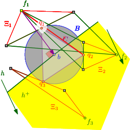
Figure 2.1: The configuration before the exchange

In each iteration, the algorithm computes the ball $B$ of minimum radius that intersects all the convex hulls $\mathcal{CH}\left({P_{1}}\right),\ldots,\mathcal{CH}\left({P_{r}}\right)$. Since $P$ is in general position, $B$ is tangent to the hulls of at most $k\leq d+1$ sets of the partition, say $\Xi_{1},\ldots,\Xi_{k}$. The $k$ sets defining this ball are tight. Let $q_{i}=B\cap\mathcal{CH}\left({\Xi_{i}}\right)$, for $i=1,\ldots,k$, and let $b$ be the center of $B$, see Figure 2.1. Observe that $b\in C=\mathcal{CH}\left({\{q_{1},\ldots,q_{k}\}}\right)$ as otherwise one can decrease the radius of $B$ by moving its center towards $C$ (which contradicts the minimality of $B$).

For $i=1,\ldots,k$, the point $q_{i}$ lies on the boundary of the simplex $\mathcal{CH}\left({\Xi_{i}}\right)$. As such, there exists a “free” point $f_{i}\in\Xi_{i}$, such that $q_{i}\in\mathcal{CH}\left({\Xi_{i}-f_{i}}\right)$. Let $h$ be the hyperplane passing through $b$ which is orthogonal to $f_{1}-b$. Let $h^{+}$ be the open halfspace bounded by $h$ that does not contain $f_{1}$. By our general position assumption, no point of $Q=\{q_{1},\ldots,q_{k}\}$ lies on $h$ (to see that, consider perturbing the points randomly, and observe that the probability for this event to happen is zero). As such, if $h^{+}\cap Q$ is empty, then $Q$ is contained in an open hemisphere $\partial B\cap h^{-}$, where $h^{-}$ is the other open halfspace bounded by $h$. But then, $B$ can be shrunk further. As such, we conclude that $Q\cap h^{+}$ is not empty. Suppose that $q_{2}$ is in this intersection, see Figure 2.2.

Figure 2.2: A beneficial exchange.

In particular, consider the exchange of $f_{1}$ and $f_{2}$:

$$\Xi_{1}^{\prime}=\Xi_{1}-f_{1}+f_{2}\qquad\text{and}\qquad\Xi_{2}^{\prime}=\Xi_{2}-f_{2}+f_{1}.$$

The segment $s=f_{1}q_{2}\subseteq\mathcal{CH}\left({\Xi_{2}^{\prime}}\right)$ intersects the interior of $B$, so $B$ can be shrunk after the exchange.

In each iteration, the radius of the ball strictly decreases. As such, the algorithm can find exchanges which allow $B$ to shrink, as long as the radius of $B$ is larger than zero. When it stops, the algorithm will have computed a partition of $P$ into sets whose convex hulls all intersect.

The ball maintained by the algorithm is uniquely defined by the $d+1$ tight sets, where each tight set contains exactly $d+1$ points. As such, the number of possible balls considered by the algorithm, and thus the number of iterations, is bounded by $O(n^{(d+1)^{2}})$. One can get a slightly better bound, by observing that the free point in each tight set is irrelevant in defining the smallest ball. As such, the number of different balls that might be computed by the algorithm is bounded by $O(n^{d(d+1)})$.

We next provide some low-level details. As a starting point, one needs the following two geometric primitives:

1. Given a point $p$ (or a ball), and a simplex in $\mathbb{R}^{d}$, compute the distance from the point to the simplex. A brute force algorithm for this works in $2^{d}d^{O(1)}$ time, as deciding if a point is in a simplex can be done in $O(d^{4})$ time by computing $d+1$ determinants. If $p$ is not in the interior of the simplex, then we recurse on each of the $d+1$ facets of the simplex, projecting $p$ to each subspace spanning this subset, and compute the nearest-point problem recursively, returning the best candidate returned. Since there are $2^{d+1}$ subsimplices, the running time stated follows.

2. Given $d+1$ simplices each defined by $d+1$ points of $P\subseteq\mathbb{R}^{d}$, the task is to compute the minimum radius ball which intersects all of them in $O(1)$ time. It can be easily written as a convex program in $O(d^{2})$ variables, which such be solved exactly in $d^{O(d^{2})}$ time. An alternative way to get a similar running time is to explicitly write down the distance function induced by each simplex, then compute the lowest point in the upper envelope of the resulting set of functions. There are $D\leq d^{O(d)}$ functions, so the complexity of the arrangement of their images is in $\mathbb{R}^{d+1}$ is $O(D^{d+1})$. This arrangement, and thus the lower point in the upper envelope, can be computed in the time stated.

At the beginning of each iteration, the algorithm computes the smallest ball intersecting the convex hulls of the sets in the current partition as follows: This is an LP type problem, and using the above geometric primitives, one can deploy any linear-time algorithm for this problem [Har11, Cla95]. The resulting running time is $d^{O(d^{2})}n$. This also returns (i) the tight sets, (ii) the ball $B$ and (iii) the points $q_{1},\ldots,q_{d+1}$. It is now straightforward to compute the free point in each simplex and do the exchange in polynomial time in $d$. Putting everything together, we get running time $n^{d(d+1)}d^{O(d^{2})}n=d^{O(d^{2})}n^{d(d+1)+1}.$  

2.3 In two dimensions

2.3.1 Computing Tukey depth in the plane

We first review Tukey depth, which is closely related to Tverberg depth in two dimensions.

Definition 2.3.

The Tukey depth of a point $q$ in a set $P\subseteq\mathbb{R}^{d}$, denoted by $\mathsf{d_{TK}}\left({q}\right)$, is the minimum number of points contained in any closed halfspace containing $q$.

The following result is implicit in the work of Chan [Cha99, Theorem 5.2]. Chan solves the decision version of the Tukey depth problem, while we need to compute it explicitly, resulting in a more involved algorithm.

Lemma 2.4.

Given a set $P$ of $n$ points in the plane and a query point $q$, such that $P\cup\{q\}$ is in general position, one can compute, in $O(n+k\log k)$ time, the Tukey depth $k$ of $q$ in $P$. The algorithm also computes the halfplane realizing this depth.

Proof:

In the dual, $q^{\star}$ is a line, and the task is to find a point on this line which minimizes the number of lines of $P^{\star}$ (i.e., set of lines dual to the points of $P$) strictly below it. More precisely, one has to also solve the upward version, and return the minimum of the two solutions. Handling the downward version first, every point $p\in P$ has a dual line $p^{\star}$. The portion of $q^{\star}$ that lies above $p^{\star}$ is a closed ray on $q^{\star}$. As such, we have a set of rays on the line (which can be interpreted as the $x$-axis), and the task is to find a point on the line contained in the minimum number of rays. (This is known as linear programming with violations in one dimension.)

Let $R_{\Mapsto}$ (resp. $L_{\Mapsfrom}$) be the set of points that corresponds to heads of rays pointing to the right (resp. to the left) by $P^{\star}$ on $q^{\star}$. Let $R_{i}$ be the set of $\left\lfloor{n/2^{i}}\right\rfloor$ rightmost points of $R_{\Mapsto}$, for $i=0,\ldots,h=\left\lfloor{\log_{2}n}\right\rfloor$. Using median selection, each set $R_{i}$ can be computed from $R_{i-1}$ in $\left|{R_{i-1}}\right|$ time. As such, all these sets can be computed in $\sum_{i}O(n/2^{i})=O(n)$ time. The sets $L_{0},L_{1},\ldots,L_{h}$ are computed in a similar fashion. For all $i$, we also compute the rightmost point $\mathcalb{r}_{i-1}$ of $R_{i-1}\setminus R_{i}$ (which is the rightmost point in $R\setminus R_{i}$). Similarly, $\mathcalb{l}_{i}$ is the leftmost point of $L_{i-1}\setminus L_{i}$, for $i=1,\ldots,h$. Let $\mathcalb{r}_{0}$ (resp. $\mathcalb{l}_{0}$) be the rightmost (resp. leftmost) point of $R_{0}$ (resp. $L_{0}$).

Now, compute the maximum $j$ such that $\mathcalb{r}_{j}$ is to the left of $\mathcalb{l}_{j}$. Observe that $(R\setminus R_{j})\cup(L\setminus L_{j})$ form a set of rays that their intersection is non-empty (i.e., feasible). Similarly, the set of rays $(R\setminus R_{j+1})\cup(L\setminus L_{j+1})$ is not feasible, and any set of feasible rays must be created by removing at least $\left|{R_{j+1}}\right|=\left|{L_{j+1}}\right|=\left\lfloor{n/2^{j+1}}\right\rfloor$ rays from $R_{\Mapsto}\cup L_{\Mapsfrom}$. Hence, in linear time, we have computed a $4$-approximation to the minimum number of rays that must be removed for feasibility. In particular, if $S$ is a set of rays such that $(R_{\Mapsto}\cup L_{\Mapsfrom})\setminus S$ is feasible, then $(R_{j-1}\cup L_{j-1})\setminus S$ is also feasible. Namely, if the minimum size of such a removeable set $S$ is $k$, then we have computed a set of $O(k)$ rays, such that it suffices to solve the problem on this smaller set.

In the second stage, we solve the problem on $R_{j-1}\cup L_{j-1}$. We first sort the points, and then for each point in this set, we compute how many rays must be removed before it lies in the intersection of the remaining rays. Given a location $p$ on the line, we need to remove all the rays of $R_{j-1}$ (resp. $L_{j-1}$) whose heads lie to the right (resp. left) of $p$. This can be done in $O(k\log k)$ time by sweeping from left to right and keeping track of the rays that need to be removed.

As such, we can solve the LP with violations on the line in $O(n+k\log k)$ time, where $k$ is the minimum number of violated constraints. A $4$-approximation to $k$ can be computed in $O(n)$ time.

Now we return to the Tukey depth problem. First we compute a $4$-approximation, denoted by $\widetilde{k_{\downarrow}}$, for the minimum number of lines crossed by a vertical ray shot down from a point on $q^{\star}$. Similarly, we compute $\widetilde{k_{\uparrow}}$. If $4\widetilde{k_{\downarrow}}<\widetilde{k_{\uparrow}}$, then we compute $k_{\downarrow}$ exactly and return the point on $q^{\star}$ that realizes it. (In the primal, this corresponds to a closed halfspace containing $q$ along with exactly $k_{\downarrow}$ points of $P$.) Similarly, if $\widetilde{k_{\downarrow}}>4\widetilde{k_{\uparrow}}$, then we compute $k_{\uparrow}$ exactly, and return it as the desired solution. In the remaining case, we compute both quantities and return the minimum of the two.  

2.3.2 Computing a log realizing the Tukey depth of a point

For shallow points in the plane, the Tukey and Tverberg depths are equivalent, and we can compute the associated Tverberg partition. This is essentially implied by the work of Birch [Bir59], and we include the details for the sake of completeness.

Lemma 2.5.

Let $P$ be a set of $n$ points in the plane, let $q$ be a query point such that $P\cup\{q\}$ is in general position, and suppose that $k=\mathsf{d_{TK}}\left({q}\right)\leq n/3$. Then one can compute a log for $q$ of rank $k$ in $O(n+k\log k)$ time.

Proof:

Using the algorithm of Lemma 2.4, compute the Tukey depth of $q$ and the closed halfplane $\mathcalb{h}^{\!\!+}$ realizing it, where $q$ lies on the line $\mathcalb{h}$ bounding $\mathcalb{h}^{\!\!+}$. This takes $O(n+k\log k)$ time. By translation and rotation, we can assume that $q$ is the origin and $\mathcalb{h}$ is the $x$-axis. Let $P^{+}=P\cap\mathcalb{h}^{\!\!+}$ be the $k$ points realizing the Tukey depth of $q$, and let $P^{-}=P\setminus P^{+}$ be the set of points below the $x$-axis, so that $\left|{P^{-}}\right|=n-k\geq 2k$.

Consider the counterclockwise order of the points of $P^{-}$ starting from the negative side of the $x$-axis. Let $T$ be the set containing the first and last $k$ points in this order, computed in $O(n)$ time by performing median selection twice. Let $T=\{t_{1},\ldots,t_{2k}\}$ be the points of $T$ sorted in counterclockwise order. Similarly, let $P^{+}=\{p_{1},\ldots,p_{k}\}$ be the points of $P^{+}$ sorted in counterclockwise order starting from the positive side of the $x$-axis, see Figure 2.3.

Figure 2.3: Illustration of the proof of Lemma 2.5.

Let $\triangle_{i}=\triangle p_{i}t_{i}t_{k+i}$, for $i=1,\ldots,k$. We claim that $q\in\triangle_{i}$ for all $i$. To this end, let $\ell_{i}$ be the line passing through the origin and $p_{i}$, and let $\ell_{i}^{+}$ denote the halfspace it induces to the left of the vector $\overrightarrow{qp_{i}}$. Then $\ell_{i}^{+}$ must contain $t_{i}$, as otherwise, $\left|{P\cap\ell_{i}^{+}}\right|<k$, contradicting the Tukey depth of $q$. Namely, the segment $p_{i}t_{i}$ intersects the negative side of the $x$-axis. A symmetric argument, applied to the complement halfplane, implies that the segment $t_{k+i}p_{i}$ intersects the positive side of the $x$-axis. Then the origin $q$ is contained in $\triangle_{i}$, as claimed.

Computing these triangles, we have found a log for $q$ of rank $k$ in $O(n+k\log k)$ time.  

The Tukey depth of a point can be as large as $\left\lfloor{n/2}\right\rfloor$. Indeed, consider the vertices of a regular $n$-gon (for odd $n$), the polygon center has depth $\left\lfloor{n/2}\right\rfloor$.

Lemma 2.6.

Let $P$ be a set of $n$ points in the plane, and let $q$ be a query point such that $P\cup\{q\}$ is in general position, and $q$ has Tukey depth larger than $n/3$. Then, one can compute, in $O(n\log n)$ time, a log for $q$ of rank $s=\left\lfloor{n/3}\right\rfloor$.

Proof:

Assume that $q$ is in the origin, and sort the points of $P$ in counterclockwise order, where $p_{i}$ is the $i$th point in this order. For $i=1,\ldots,s$, let $\triangle_{i}=\triangle p_{i}p_{s+i}p_{2s+i}$. We claim that $\angle p_{i}qp_{s+i}\leq\pi$. Otherwise, there is a halfspace containing fewer than $s$ points induced by the line passing through $p_{i}$ and $q$. Similarly, $\angle p_{s+i}qp_{2s+i}\leq\pi$ and $\angle p_{2s+i}qp_{i}\leq\pi$, so that $q$ lies inside $\triangle_{i}$, as desired.  

Theorem 2.7.

Let $P$ be a set of $n$ points in the plane, let $q$ be a query point such that $P\cup\{q\}$ is in general position, and suppose that $k=\mathsf{d_{TK}}\left({q}\right)$ is the Tukey depth of $q$ in $P$. Then one can compute the Tukey depth $k$ of $q$, along with a log of rank $\tau=\min(\left\lfloor{n/3}\right\rfloor,k)$, in $O(n+k\log k)$ time.

Proof:

Compute the Tukey depth of $q$ in $O(n+k\log k)$ time, using the algorithm of Lemma 2.4. If $k\leq n/3$, then compute the log using the algorithm of Lemma 2.5, and otherwise using the algorithm of Lemma 2.6.  

The above implies the following theorem of Birch, which predates Tverberg’s theorem.

Theorem 2.8 ([Bir59]).

Let $P$ be a set of $n=3k$ points in the plane. Then there exists a partition of $P$ into $k$ vertex-disjoint triangles, such that their intersection is not empty. The partition can be computed in $O(n\log n)$ time.

Proof:

A centerpoint of $P$ can be computed in $O(n\log n)$ time [Cha04]. Such a centerpoint has Tukey depth at least $k$, so the algorithm of Lemma 2.6 partitions $P$ into $k$ triangles.  

Remark 2.9.

(A) Note that Tverberg’s theorem in the plane is slightly stronger – it states that any point set with $3k-2$ points has Tverberg depth $k$. In such a decomposition, some of the sets may be pairs of points or singletons.

(B) In the colored version of Tverberg’s theorem in the plane, one is given $3n$ points partitioned into three classes of equal size. Agarwal et al. [ASW08] showed how to compute a decomposition into $n$ triangles covering a query point, where every triangle contains a vertex of each color (if such a decomposition exists). This problem is significantly more difficult, and their running time is a prohibitive $O(n^{11})$.

2.4 Miller and Sheehy’s algorithm

Here, we review Miller and Sheehy’s approximation algorithm [MS10] for computing a Tverberg point before describing our improvement.

Radon partitions.

Radon’s theorem states that a set $P$ of $d+2$ points in $\mathbb{R}^{d}$ can be partitioned into two disjoint subsets $P_{1},P_{2}$ such that $\mathcal{CH}\left({P_{1}}\right)\cap\mathcal{CH}\left({P_{2}}\right)\neq\emptyset$. This partition can be computed via solving a linear system in $d+2$ variables in $O(d^{3})$ time. A point in this intersection (which is an immediate byproduct of computing the partition) is a Radon point.

Let $p$ be a point in $\mathbb{R}^{d}$. It is a convex combination of points $\{p_{1},\ldots,p_{m}\}$ if there are $\alpha_{1},\ldots,\alpha_{m}\in[0,1]$ such that $p=\sum_{i=1}^{m}\alpha_{i}p_{i}$ and $\sum_{i}\alpha_{i}=1$.

Lemma 2.10 ([MS10]: Sparsifying convex combination).

Let $p$ be a point in $\mathbb{R}^{d}$, and let $P=\{p_{1},\ldots,p_{m}\}\subseteq\mathbb{R}^{d}$ be a point set. Furthermore, assume that we are given $p$ as a convex combination of points of $P$. Then, one can compute a convex combination representation of $p$ that uses at most $d+1$ points of $P$. This takes $O(md^{3})$ time.

Proof:

Assume that we are given $\alpha_{1},\ldots,\alpha_{m}\in[0,1]$, $\sum_{i}\alpha_{i}=1$, such that $p=\sum_{i=1}^{m}\alpha_{i}p_{i}$, One can now sparsify the set $P$ so that it contains only $d+1$ points. Indeed, if any point of $P$ has zero coefficient in the representation of $p$ then it can be deleted. If there are more than $d+1$ points with non-zero coefficient, then pick $d+2$ of them, say $p_{1},\ldots,p_{d+2}$. Computing their Radon decomposition, we get convex coefficients $\alpha_{1},\ldots,\alpha_{k},\beta_{k+1},\ldots,\beta_{d+2}\in[0,1]$, such that $\sum_{i}\alpha_{i}=1$, $\sum_{i}\beta_{i}=1$, and $\sum_{i}\alpha_{i}p_{i}+\sum_{i=k+1}^{d+2}-\beta_{i}p_{i}=0$. Subtracting this equation from the current representation of $p$ (scaled with the appropriate constant) yields a representation of $p$ as a convex combination with more zero coefficients. This takes $O(d^{3})$ time, and repeating it at most $m-d$ times results in the desired reduced set of size $d+1$. The process takes $O(d^{3}m)$ time overall.  

Lemma 2.11 ([MS10]: Merging logs).

Given $d+2$ sites $(p_{1},\mathcalb{l}_{1}),$ $\ldots,(p_{d+2},\mathcalb{l}_{d+2})$ of rank $r$ in $\mathbb{R}^{d}$, where the logs $\mathcalb{l}_{i}$ are disjoint, one can compute a site $(p,\mathcalb{l})$ of rank $2r$ in $O(rd^{5})$ time.

Proof:

Let $p$ be the Radon point of $p_{1},\ldots,p_{d+2}$, and let the Radon partition be given by $P_{1}=\{p_{1},\ldots,p_{k}\}$ and $P_{2}=\{p_{k+1},\ldots,p_{d+2}\}$. Picking the first set $Q_{i}$ in the long $\mathcalb{l}_{i}$, for $i=1,\ldots,k$, results in a set $\cup Q_{i}$ of size $O(d^{2})$, whose convex hull contains $\mathcal{CH}\left({P_{1}}\right)$. It also contains $p$, as $p\in\mathcal{CH}\left({P_{1}}\right)\cap\mathcal{CH}\left({P_{2}}\right)$.

Since every log contains $r$ sets, we can repeat this process $r$ times. we thus get $r$ disjoint sets, each of size $O(d^{2})$, from the logs of the points of $P_{1}$, and each of their convex hulls contains $p$. Similarly, we get a similar log of size $r$ from $P_{2}$, and the union of the two logs is the desired new log of $p$ of rank $2r$. It is straightforward to compute the convex representation of $p$ in these new logs.

The only issue is that each set $Q$ in the new log has size $O(d^{2})$. We now sparsify every such set using Lemma 2.10. This takes $O(d^{5})$ time per set, and $O(d^{5}r)$ time overall.  

A recycling algorithm for computing a Tverberg point.

The algorithm of Miller and Sheehy maintains a collection of sites. Initially, it converts each input point $p\in P$ into a site $(p,\{p\})$ of rank one. The algorithm then merges $d+2$ sites of rank $r$ into a site of rank $2r$, using Lemma 2.11. Before the merge, the input logs use $r(d+2)(d+1)$ points in total. After the merge, the new log uses only $2(d+1)r$ points. The algorithm recycles the remaining $(d+2)(d+1)r-2(d+1)r=d(d+1)r$ points by reinserting them into the collection as singleton sites of rank one. When no merges are available, the algorithm outputs the maximum-rank site as the approximate Tverberg point.

Analysis.

For our purposes, we need a slightly different way of analyzing the above algorithm of Miller and Sheehy [MS10], so we provide the analysis in detail.

Lemma 2.12.

Let $2^{h}$ be the rank of the output site. For $n\geq 8d(d+1)^{2}$, we have that

$$\left\lceil{\frac{n}{2(d+1)^{2}}}\right\rceil\leq 2^{h}\leq\frac{2n}{(d+1)^{2}}.$$

Proof:

Consider the logs when the algorithm stopped. The number of points in all the logs is $n$. Since a site of rank $2^{i}$ has at most $(d+1)2^{i}$ points of $P$ in its log, and there are at most $d+1$ sites of each rank, $n$ is at most $\sum_{i=0}^{h}(d+1)^{2}2^{i}$. As such,

$$n\leq\sum_{i=0}^{h}(d+1)^{2}2^{i}=(d+1)^{2}(2^{h+1}-1)\iff\frac{n}{(d+1)^{2}}+1\leq 2^{h+1}\implies 2^{h}\geq\left\lceil{\frac{n}{2(d+1)^{2}}}\right\rceil.$$ (2.1)

As for the lower bound, consider the logs just before the output site was computed. There are $d+2$ sites, each of rank $2^{h-1}$. Each of their logs contains $(d+1)2^{h-1}$ points. Here, we use the lower bound on $n$, as a batch in a log of a site of rank smaller than (say) $2d$ can have fewer elements. However, under general position assumption, the way the above algorithm works, once the rank is sufficiently large (i.e., $>d+1$), it must be that each batch in the log indeed contains $d+1$ points. Indeed, initially, a batch is of size one. If the site if of rank $2^{i}$, then a batch for it is formed by the union of $2^{i}$ original batches (i.e., at least $2^{i}$ points) – the algorithm then trims such a set to be of size $d+1$. Once a site gets to be of sufficiently high rank, under general position assumption, it is not going to lie on a $k$ dimensional subspace induced by $k+1$ original points of $P$, for $k<d$ (indeed, just consider slightly perturbing the points – the probability for this to happen is zero). As such, we conclude that $n\geq(d+1)(d+2)2^{h-1}$. This implies that $2^{h}\leq 2n/\bigl{(}(d+1)(d+2)\bigr{)}\leq 2n/(d+1)^{2}.$  

Every site in the collection is associated with a history tree that describes how it was computed. Thus, the algorithm execution generates (conceptually) a forest of such history trees, which is the history of the computation.

Lemma 2.13.

Let $2^{h}$ be the maximum rank of a site computed by the algorithm. The total number of sites in the history that are of rank (exactly) $2^{h-i}$ is at most $(d+2)^{i+1}-1$.

Proof:

There are at most $T(0)=d+1$ nodes of rank $2^{h-0}$ in the history, and each has $d+2$ children of rank $2^{h-1}$. In addition, there might be $d+1$ trees in the history whose roots have rank $2^{h-1}$. Thus,

$$T(1)=d+1+(d+2)T(0)=(d+1)+(d+2)(d+1)=(d+3)(d+1)=(d+2)^{2}-1.$$

Assume that $T(i-1)=(d+2)^{i}-1$. By induction, there are at most

$$T(i)=d+1+(d+2)T(i-1)=d+1+(d+2)\bigl{(}(d+2)^{i}-1\bigr{)}=(d+2)^{i+1}-1$$

nodes in the history of rank $2^{h-i}$.  

Lemma 2.14.

Let $2^{h}$ be the maximum rank of a site computed by the algorithm. The total amount of work spent (directly) by the algorithm (throughout its execution) at nodes of rank $\geq 2^{h-i}$ is $O(d^{4+i}n).$ In particular, the overall running time of the algorithm is $O(d^{4}n^{1+\log_{2}d})$.

Proof:

Bu Lemma 2.13, there are at most $(d+2)^{i+1}$ nodes of rank $2^{h-i}$ in the history. By Lemma 2.12, the rank of such a node is

$$r_{i}=\frac{2^{h}}{2^{i}}\leq\frac{2n}{2^{i}(d+1)^{2}},$$

and the amount of work spent in computing the node is $O(r_{i}d^{6})=O\left({d^{4}n/2^{i}}\right).$ As such, the total work in the top $i$ ranks of the history is proportional to $L_{i}=\sum_{j=0}^{i}(d+2)^{j}\cdot d^{4}n/2^{j}=O(d^{4+i}n).$

Since $h\leq\log_{2}n$, the overall running time is $O(L_{h})=O(d^{4+\log_{2}n}n)=O(d^{4}n^{1+\log_{2}d})$.  

3 Improved Tverberg approximation algorithms

3.1 Projections in low dimensions

Lemma 3.1.

Let $P$ be a set of $n$ points in three dimensions. One can compute a Tverberg point of $P$ of depth $n/6$ (and the log realizing it) in $O(n\log n)$ time.

Proof:

Project the points of $P$ to two dimensions, and compute a Tverberg point $p$ and a partition for it of size $n/3$, using Theorem 2.8. Lifting from the plane back to the original space, the point $p$ lifts to a vertical line $\ell$, and every triangle lifts to a triangle that intersects $\ell$. Pick a point $q$ on this line which is the median of the intersections. Now, pair every triangle intersecting $\ell$ above $q$ with a triangle intersecting $\ell$ below it. This partitions $P$ into $n/6$ sets, each of size $6$, such that the convex hull of each sets contains $q$. Within each set, compute at most $4$ points whose convex hull contains $q$. These points yield the desired log for $q$ of rank $n/6$.  

Remark 3.2.

Lemma 3.1 seems innocent enough, but to the best of our knowledge, it is the best one can do in near-linear time in 3D. The only better approximation algorithm we are aware of is the one suggested by Tverberg’s theorem. It yields a point of Tverberg depth $n/4$, but its running time is $O(n^{13})$ (see Lemma 2.2).

As observed by Mulzer and Werner [MW13], one can repeat this projection mechanism. Since Mulzer and Werner [MW13] bottom their recursion at dimension $1$, their algorithm computes a point of Tverberg depth $n/2^{d}$ (in three dimensions, depth $n/8$). Applying this projection idea but bottoming at two dimensions, as above, yields a point of Tverberg depth $n/(3\cdot 2^{d-2})$.

Lemma 3.3.

Let $P$ be a set of $n$ points in four dimensions. One can compute a Tverberg point of $P$ of depth $n/9$ (and the log realizing it) in $O(n\log n)$ time.

More generally, for $d$ even, and a set $P$ of $n$ points in $\mathbb{R}^{d}$, one can compute a point of depth $n/3^{d/2}$ in $d^{O(1)}n\log n$ time. For $d$ odd, we get a point of depth $n/(2\cdot 3^{(d-1)/2})$.

Proof:

As mentioned above, the basic idea is due to Mulzer and Werner. Project the four-dimensional point set onto the plane spanned by the first two coordinates (i.e. “eliminate” the last two coordinates), and compute a $n/3$ centerpoint using Theorem 2.8. Translate the space so that this centerpoint lies at the origin. Now, consider each triangle in the original four-dimensional space. Each triangle intersects the two-dimensional subspace formed by the first two coordinates. Pick an intersection point from each lifted triangle. On this set of $n/3$ points, living in this two dimensional subspace, apply again the algorithm of Theorem 2.8 to compute a Tverberg point of depth $(n/3)/3=n/9$. The resulting centerpoint $p$ is now contained in $n/9$ triangles, where every vertex is contained in an original triangle of points. That is, $p$ has depth $n/9$, where each group consists of $9$ points in four dimensions. Now, sparsify each group into $5$ points whose convex hull contains $p$.

The second part of the claim follows from applying the above argument repeatedly.  

3.2 An improved quasi-polynomial algorithm

The algorithm of Miller and Sheehy is expensive at the bottom of the recursion tree, so we replace the bottom with a faster algorithm. We use the following result of Mulzer and Werner.

Theorem 3.4 ([MW13]).

Given a set $P$ of $n$ points in $\mathbb{R}^{d}$, one can compute a site of rank $\geq n/4(d+1)^{3}$ (together with its log) in $d^{O(\log d)}n$ time.

Let $\delta\in(0,1)$ be a small constant. We modify the algorithm of Miller and Sheehy by keeping all the singleton sites of rank one in a buffer of free points. Initially, all points are in the buffer. Whenever the buffer contains at least $\delta n$ points, we use the algorithm of Theorem 3.4 to compute a site of rank $\rho\geq\delta n/8(d+1)^{3}$, where $\rho$ is a power of two. (If the computed rank is too large, we throw away entries from the log until the rank reaches a power of two.) We insert this site into the collection of sites maintained by the algorithm. As in Miller and Sheehy’s algorithm, we repeatedly merge $d+2$ sites of the same rank to get a site of double the rank. In the process, the points thrown out from the log are recycled into the buffer. Whenever the buffer size exceeds $\delta n$, we compute a new site of rank $\rho$. This process stops when no sites can be merged and the number of free points is less than $\delta n$.

Theorem 3.5.

Given a set $P$ of $n$ points in $\mathbb{R}^{d}$, and a parameter $\delta\in(0,1)$, one can compute a site of rank at least $\frac{(1-\delta)n}{2(d+1)^{2}}$ (together with its log) in $d^{O(\log(d/\delta))}n$ time.

Proof:

When the algorithm above stops, there are at least $(1-\delta)n$ points in its logs. Arguing as in Lemma 2.12, the output site has rank

$$2^{h}\geq\frac{(1-\delta)n}{2(d+1)^{2}}.$$

We now consider the running time. The algorithm maintains only nodes of rank $\rho\geq 2^{h-H}$, where

$$H=\left\lceil{\log_{2}\frac{2^{h}}{\rho}}\right\rceil\leq\left\lceil{\log_{2}\frac{n/2(d+1)^{2}}{\delta n/8(d+1)^{3}}}\right\rceil=1+\log_{2}\frac{4(d+1)}{\delta}=O(\log(d/\delta)).$$

The total work spent on merging nodes with these ranks is equivalent to the work in Miller and Sheehy’s algorithm for such nodes. By Lemma 2.14, the total work performed is $O(d^{4+H}n)$.

As for the work associated with the buffer, observe that Theorem 3.4 is invoked $(d+2)^{H+1}$ times (this is the number of nodes in the history of rank $2^{h-H}$). Each invocation takes $d^{O(\log d)}n$ time, so the total running time of the algorithm is

$$d^{O(H)}n+(d+1)^{H+1}d^{O(\log d)}n=d^{O(\log(d/\delta))}n.$$

 

3.3 A strongly polynomial algorithm

Lemma 3.6.

Let $P$ be a set of $n$ points in $\mathbb{R}^{d}$. For $N=\Theta(d^{2}\log d)$, consider a random coloring of $P$ by $k=\left\lfloor{n/N}\right\rfloor$ colors, and let $\{P_{1},\ldots,P_{k}\}$ be the resulting partition of $P$. With probability $\geq 1-k/d^{O(d)}$, this partition is a Tverberg partition of $P$ – that is, $\cap_{i}\mathcal{CH}\left({P_{i}}\right)\neq\emptyset$.

Proof:

Let ${\varepsilon}=1/(d+1)$. The VC dimension of halfspaces in $\mathbb{R}^{d}$ is $d+1$ by Radon’s theorem. By the ${\varepsilon}$-net theorem [HW87, Har11], a sample from $P$ of size

$$N=\left\lceil{\frac{8(d+1)}{{\varepsilon}}\log(16(d+1))}\right\rceil=\Theta(d^{2}\log d)$$

is an ${\varepsilon}$-net with probability $\geq 1-4\bigl{(}16(d+1)\bigr{)}^{-2(d+1)}$. Thus $P_{1},\ldots,P_{k}$ are all ${\varepsilon}$-nets with the probability stated in the lemma.

Now, consider the centerpoint $q$ of $P$. We claim that $q\in\mathcal{CH}\left({P_{i}}\right)$, for all $i$. Indeed, assume otherwise, so that there is a separating hyperplane between $q$ and some $P_{i}$. Then the halfspace induced by this hyperplane that contains $q$ also contains at least ${\varepsilon}n$ points of $P$, because $q$ is a centerpoint of $P$. But this contradicts that $P_{i}$ is an ${\varepsilon}$-net for halfspaces.  

Lemma 3.7.

Let $P$ be a set of $n$ points in $\mathbb{R}^{d}$. For $N=O(d^{3}\log d)$, consider a random coloring of $P$ by $k=\left\lfloor{n/N}\right\rfloor=\Omega(\frac{n}{d^{3}\log d})$ colors, and let $\{P_{1},\ldots,P_{k}\}$ be the resulting partition of $P$. One can compute, in $O(d^{7}\log^{6}d)$ time, a Tverberg point that lies in $\bigcap_{i}\mathcal{CH}\left({P_{i}}\right)$. This algorithm succeeds with probability $\geq 1-k/d^{O(d)}$.

Proof:

Compute a $1/(2d^{2})$-centerpoint $q$ for $P$ using the algorithm of Har-Peled and Jones [HJ19], and repeat the argument of Lemma 3.6 with ${\varepsilon}=1/(2d^{2})$. With the desired probability, $q\in\mathcal{CH}\left({P_{i}}\right)$ for all $i$.  

3.4 A weakly polynomial algorithm

Let $T_{\textsf{LP}}\left({n,m}\right)$ be the time to solve an LP with $n$ variables and $m$ constraints. Using interior point methods, one can solve such LPs in weakly polynomial time. The fastest known method runs in $\mathcal{O}_{w}(mn+n^{3})$ [BLSS20] or $\mathcal{O}_{w}(mn^{3/2})$ [LS15], where $\mathcal{O}_{w}$ hides polylogarithmic terms that depends on $n,m$, and the width of the input numbers.

Remark 3.8.

The error of the LP solver, see [BLSS20], for a prescribed parameter ${\varepsilon}$, is the distance of the computed solution from an optimal one. Specifically, let $R$ be the maximum absolute value of any number in the given instance. In $O((nm+n^{3})\log^{O(1)}n\log(n/{\varepsilon}))$ time, the LP solver can find an assignment to the variables which is $\mathcal{E}$ close to complying with the LP constraints, where $\mathcal{E}\leq{\varepsilon}nmR$ [BLSS20]. That is, the LP solver can get arbitrarily close to a true solution. This is sufficient to compute an exact solution in polynomial time if the input is made out of integer numbers with polynomially bounded values, as the running time then depends on the number of bits used to encode the input. We use $\mathcal{O}_{w}(\cdot)$ to denote such weakly polynomial running time.

Lemma 3.9 (Carathéodory via LP).

Given a set $P$ of $n$ points in $\mathbb{R}^{d}$ and query point $q$, one can decide if $q\in\mathcal{CH}\left({P}\right)$, and if so, output a convex combination of $d+1$ points of $P$ that is equal to $q$. The running time of this algorithm is $O(T_{\textsf{LP}}\left({n,n+d}\right)+nd^{3})=\mathcal{O}_{w}(nd+nd^{3})$.

Alternatively, one can compute such a point in $2^{O(\sqrt{d\log d})}+O(d^{2}n)$ time.

Proof:

We write the natural LP for representing $q$ as a point in the interior of $\mathcal{CH}\left({P}\right)$. This LP has $n$ variables (one for each point), and $n+2d+2$ constraints (all variables are positive, the points sum to $q$, and the coefficients sum to $1$), where an equality constraint counts as two constraints. If the LP computes a solution, then we can sparsify it using Lemma 2.10.

The alternative algorithm writes an LP to find a hyperplane separating $q$ from $P$. First, it tries to find a hyperplane which is vertically below $P$ and above $q$. This LP has $d$ variables, and it can be solved in $O(2^{\sqrt{d\log d}}+d^{2}n)$ time [Sei91, Cla95, MSW96]. If there is no such separating hyperplane, then the algorithm provides $d$ points whose convex hull lies below $q$ and tries again. This time, it computes a separating hyperplane below $q$ and above $P$. Again, if no such separating hyperplane exists, then the algorithm returns $d$ points whose convex hull lies above $q$. The union of the computed point sets above and below $q$ contains at most $2d$ points. Now, write the natural LP with $2d$ variables as above, and solve it using linear-time LP solvers in low dimensions. This gives the desired representation.  

Remark 3.10.

Rolnick and Soberón [RS16] achieved a result similar to that of Lemma 3.9, but they used binary search to find the $d+1$ coefficients in the minimal representation. Thus their running time is (slightly worse) $O(T_{\textsf{LP}}\left({n,n+d}\right)d\log n)$.

Using Lemma 3.6, we get the following.

Lemma 3.11.

Let $P$ be a set of $n$ points in $\mathbb{R}^{d}$. For $N=O(d^{2}\log d)$, one can compute a site $q$ of rank $k=n/O(d^{2}\log d)$ in $\mathcal{O}_{w}(n^{5/2}+nd^{3})$ time. The algorithm succeeds with probability $\geq 1-k/d^{O(d)}$.

Proof:

We compute a Tverberg partition using Lemma 3.6. Next we write an LP for computing an intersection point $q$ that lies in the interior of the $k=n/O(d^{2}\log d)$ sets. This LP has $O(n+d)$ constraints and $n$ variables, and it can be solved in $\mathcal{O}_{w}(n^{5/2})$ time [LS15]. We then sparsify the representations over each of the $k$ sets. This requires $O(d^{2}\log d\cdot d^{3})$ time per set and hence $O(nd^{3})$ time overall. The result is a site $q$ with a log of rank $k$, as desired.  

Theorem 3.12.

Given a set $P$ of $n$ points in $\mathbb{R}^{d}$, and a parameter $\delta\in(0,1)$, one can compute a site of rank at least $\frac{(1-\delta)n}{2(d+1)^{2}}$ (together with its log) in $d^{O(\log\log(d/\delta))}\mathcal{O}_{w}(n^{5/2})$ time.

Proof:

We modify the algorithm of Theorem 3.5 to use Lemma 3.11 to compute a Tverberg point on the points in the buffer. Since the gap between the top rank of the recursion tree and rank computed by Lemma 3.11 is $O(\log(d/\delta))$, it follows that the algorithm uses only the top $O(\log\log(d/\delta))$ levels of the recursion tree, and the result follows.  

3.5 Faster approximation in low dimensions

Lemma 3.13.

Let $P$ be a set of $n$ points in $\mathbb{R}^{d}$, and let $\delta\in(0,1)$ be some parameter. One can compute a Tverberg point of depth $\geq(1-\delta)n/d(d+1)$, together with its log, in $O(d^{O(d)}/\delta^{2(d-1)}+2^{O(\sqrt{d\log d})}n+d^{2}n\log^{2}n)$ time. The algorithm succeeds with probability close to one.

Proof:

Let ${\varepsilon}=1/2(d+1)$, and let $R$ be a random sample from $P$ of size

$$m=O(d{\varepsilon}^{-1}\delta^{-2}\log{\varepsilon}^{-1})=O(d^{2}\delta^{-2}\log d).$$

This sample is a $({\varepsilon},\delta)$-relative approximation for $P$ with probability close to one [HS11]. Compute a centerpoint $c$ for the sample using “brute force” in $O(m^{d-1})$ time [Cha04]. Now, repeatedly use the algorithmic version of Carathéodory’s theorem (Lemma 3.9) to extract a simplex that contains $c$. One can repeat this process $\left\lfloor{n/d(d+1)}\right\rfloor$ times before getting stuck, since every simplex contains at most $d$ points in any halfspace passing through $c$. Naively, the running time of this algorithm is $2^{O(\sqrt{d\log d})}n^{2}$.

However, one can do better. The number of simplices extracted by the above algorithm is $L=\left\lfloor{n/d(d+1)}\right\rfloor$. For $i=1,\ldots L$, let $b_{i}=\left\lfloor{n/(d+1)}\right\rfloor-d(i-1)$ be a lower bound on the Tukey depth of $c$ at the beginning of the $i$th iteration of the above extraction algorithm. At this moment, the point set has $n_{i}=n-(d+1)(i-1)\geq n/2$ points. Hence the relative Tukey depth of $c$ is ${\varepsilon}_{L-i}={b_{L-i}}/{n_{L-i}}.$ In particular, an ${\varepsilon}_{i}$-net $R_{i}$ for halfspaces has size $r_{i}=O(\frac{d}{{\varepsilon}_{i}}\log\frac{1}{{\varepsilon}_{i}}).$ If $r_{i}$ is larger than the number of remaining points, then the sample consists of the remaining points of $P$. The convex hull of such a sample contains $c$ with probability close to one, so one can apply Lemma 3.9 to $R_{i}$ to get a simplex that contains $P$ (if the sample fails, then the algorithm resamples). The algorithm adds the simplex to the output log, removes its vertices from $P$, and repeats.

Since the algorithm invokes Lemma 3.9 $O(n/d^{2})$ times, the running time is bounded by $2^{O(\sqrt{d\log d})}n/d^{2}+O(d^{2}\sum_{i}r_{i}).$ Since $n_{L-i}\geq n/2$ and $b_{L-i}\geq i\cdot d$, we have that ${\varepsilon}_{L-i}\geq(id/(n/2)=2id/n$. Therefore,

$$\sum_{i}r_{i}=O(n)+\sum_{i=1}^{L-1}r_{L-i}=O(n)+\sum_{i=1}^{L-1}O\left({\frac{dn}{2id}\log\frac{n}{id}}\right)=O(n\log^{2}n).$$

 

Acknowledgments.

The authors thank Timothy Chan, Wolfgang Mulzer, David Rolnick, and Pablo Soberon-Bravo for providing useful references.

References

- [AHS+17] Pankaj K. Agarwal et al. “Convex Hulls Under Uncertainty” In Algorithmica 79.2, 2017, pp. 340–367 DOI: 10.1007/s00453-016-0195-y
- [ASS15] Peyman Afshani, Donald R. Sheehy and Yannik Stein “Approximating the Simplicial Depth” In CoRR abs/1512.04856, 2015 arXiv: http://arxiv.org/abs/1512.04856
- [ASW08] Pankaj K. Agarwal, Micha Sharir and Emo Welzl “Algorithms for center and Tverberg points” In ACM Trans. Algo. 5.1, 2008, pp. 5:1–5:20 DOI: 10.1145/1435375.1435380
- [Avi93] David Avis “The -core properly contains the -divisible points in space” In Pattern Recognit. Lett. 14.9, 1993, pp. 703–705 DOI: 10.1016/0167-8655(93)90138-4
- [Bir59] B.. Birch “On 3N points in a plane” In Mathematical Proceedings of the Cambridge Philosophical Society 55.4 Cambridge University Press, 1959, pp. 289–293 DOI: 10.1017/S0305004100034071
- [BLSS20] Jan Brand, Yin Tat Lee, Aaron Sidford and Zhao Song “Solving tall dense linear programs in nearly linear time” In Proc. 52nd Annu. ACM Sympos. Theory Comput. (STOC) ACM, 2020, pp. 775–788 DOI: 10.1145/3357713.3384309
- [CEM+96] Kenneth L. Clarkson et al. “Approximating center points with iterative Radon points” In Int. J. Comput. Geom. Appl. 6, 1996, pp. 357–377 DOI: 10.1142/S021819599600023X
- [Cha04] T.. Chan “An optimal randomized algorithm for maximum Tukey depth” In Proc. 15th ACM-SIAM Sympos. Discrete Algs. (SODA) SIAM, 2004, pp. 430–436 URL: http://dl.acm.org/citation.cfm?id=982792.982853
- [Cha85] B. Chazelle “On the convex layers of a planar set” In IEEE Trans. Inform. Theory IT-31.4, 1985, pp. 509–517 DOI: 10.1109/TIT.1985.1057060
- [Cha99] T.. Chan “Geometric applications of a randomized optimization technique” In Disc. Comput. Geom. 22.4, 1999, pp. 547–567 DOI: 10.1007/PL00009478
- [Cla95] K.. Clarkson “Las Vegas algorithms for linear and integer programming” In J. Assoc. Comput. Mach. 42, 1995, pp. 488–499 DOI: 10.1145/201019.201036
- [CM20] Aruni Choudhary and Wolfgang Mulzer “No-Dimensional Tverberg Theorems and Algorithms” In Proc. 36th Int. Annu. Sympos. Comput. Geom. (SoCG) 164, LIPIcs Schloss Dagstuhl - Leibniz-Zentrum für Informatik, 2020, pp. 31:1–31:17 DOI: 10.4230/LIPIcs.SoCG.2020.31
- [Dal04] Ketan Dalal “Counting the onion” In Random Struct. Alg. 24.2, 2004, pp. 155–165 DOI: 10.1002/rsa.10114
- [Har11] Sariel Har-Peled “Geometric Approximation Algorithms” American Mathematical Society, 2011
- [HJ19] Sariel Har-Peled and Mitchell Jones “Journey to the Center of the Point Set” In Proc. 35th Int. Annu. Sympos. Comput. Geom. (SoCG) 129, LIPIcs Schloss Dagstuhl - Leibniz-Zentrum fuer Informatik, 2019, pp. 41:1–41:14 DOI: 10.4230/LIPIcs.SoCG.2019.41
- [HL13] S. Har-Peled and B. Lidicky “Peeling the grid” In SIAM J. Discrete Math. 27.2, 2013, pp. 650–655 DOI: 10.1137/120892660
- [HS11] S. Har-Peled and M. Sharir “Relative -Approximations in Geometry” In Disc. Comput. Geom. 45.3, 2011, pp. 462–496 DOI: 10.1007/s00454-010-9248-1
- [HW87] D. Haussler and E. Welzl “-nets and simplex range queries” In Disc. Comput. Geom. 2, 1987, pp. 127–151 DOI: 10.1007/BF02187876
- [JM94] Shreesh Jadhav and Asish Mukhopadhyay “Computing a Centerpoint of a Finite Planar Set of Points in Linear Time” In Disc. Comput. Geom. 12, 1994, pp. 291–312 DOI: 10.1007/BF02574382
- [LS15] Yin Tat Lee and Aaron Sidford “Efficient Inverse Maintenance and Faster Algorithms for Linear Programming” In Proc. 56th Annu. IEEE Sympos. Found. Comput. Sci. (FOCS) IEEE Computer Society, 2015, pp. 230–249 DOI: 10.1109/FOCS.2015.23
- [MMSS17] Frédéric Meunier, Wolfgang Mulzer, Pauline Sarrabezolles and Yannik Stein “The Rainbow at the End of the Line - A PPAD Formulation of the Colorful Carathéodory Theorem with Applications” In Proc. 28th ACM-SIAM Sympos. Discrete Algs. (SODA) SIAM, 2017, pp. 1342–1351 DOI: 10.1137/1.9781611974782.87
- [MS10] Gary L. Miller and Donald R. Sheehy “Approximate centerpoints with proofs” In Comput. Geom. 43.8, 2010, pp. 647–654 DOI: 10.1016/j.comgeo.2010.04.006
- [MSW96] J. Matoušek, M. Sharir and E. Welzl “A Subexponential Bound for Linear Programming” In Algorithmica 16.4/5, 1996, pp. 498–516 DOI: 10.1007/BF01940877
- [MW13] Wolfgang Mulzer and Daniel Werner “Approximating Tverberg Points in Linear Time for Any Fixed Dimension” In Disc. Comput. Geom. 50.2, 2013, pp. 520–535 DOI: 10.1007/s00454-013-9528-7
- [Rea79] John R. Reay “Several generalizations of Tverberg’s theorem” In Israel Journal of Mathematics 34.3, 1979, pp. 238–244 DOI: 10.1007/BF02760885
- [RS16] David Rolnick and Pablo Soberón “Algorithms for Tverberg’s theorem via centerpoint theorems” In CoRR abs/1601.03083, 2016 arXiv: http://arxiv.org/abs/1601.03083v2
- [Sei91] R. Seidel “Small-dimensional linear programming and convex hulls made easy” In Disc. Comput. Geom. 6, 1991, pp. 423–434 DOI: 10.1007/BF02574699
- [TV93] Helge Tverberg and Siniša Vrećica “On Generalizations of Radon’s Theorem and the Ham Sandwich Theorem” In Euro. J. Combin. 14.3, 1993, pp. 259–264 DOI: https://doi.org/10.1006/eujc.1993.1029