Understanding and Diagnosing
Vulnerability under Adversarial Attacks

Abstract

Deep Neural Networks (DNNs) are known to be vulnerable to adversarial attacks. Currently, there is no clear insight into how slight perturbations cause such a large difference in classification results and how we can design a more robust model architecture. In this work, we propose a novel interpretability method, InterpretGAN, to generate explanations for features used for classification in latent variables. Interpreting the classification process of adversarial examples exposes how adversarial perturbations influence features layer by layer as well as which features are modified by perturbations. Moreover, we design the first diagnostic method to quantify the vulnerability contributed by each layer, which can be used to identify vulnerable parts of model architectures. The diagnostic results show that the layers introducing more information loss tend to be more vulnerable than other layers. Based on the findings, our evaluation results on MNIST and CIFAR10 datasets suggest that average pooling layers, with lower information loss, are more robust than max pooling layers for the network architectures studied in this paper.

1 Introduction

Deep Neural Networks (DNNs) have been found to be vulnerable to adversarial attacks [1]. Even slight imperceptible perturbations can lead to model misclassification. To mitigate adversarial attacks, various types of defense methods [2, 3, 4, 5, 6, 7, 8, 9] are proposed. Besides building defense methods, recent research also tries to interpret the reason behind the adversarial attack. Ilyas et al. [10] showed that DNNs tend to use non-robust features for classification, rather than robust features. Another work [11] applied network dissection [12] to interpret adversarial examples. However, there is no clear understanding of the reason behind the vulnerability to adversarial attacks. Since latent variables in DNNs are usually uninterpretable, it is difficult to explain how adversarial perturbations influence features in latent variables and result in final misclassification.

If features influenced by perturbations can be translated to natural image space, we can understand which features are influenced in latent variables. To achieve this goal, we propose a novel interpretability method, InterpretGAN, that can generate explanations for features relevant to classification in latent variables. In InterpretGAN, we apply a Generative Adversarial Network (GAN) to train the explanation generator so that generated explanations follow a training data distribution and are interpretable. In order for explanations to contain the necessary features used for classification, we introduce an interpretability term for GAN training that ensures mutual information between explanations and classification results. Whenever adversarial perturbations distort features used for classification, InterpretGAN can reflect those changes in the explanations.

We interpret the classification process of models trained on MNIST [13] and CelebFaces [14] (with gender as the label) datasets and use InterpretGAN to generate explanations for each layer of the two models. Based on generated explanations, we discover several interesting findings. For classification of natural images, we find that as latent variables are processed layer by layer, features irrelevant to classification (e.g., hat for gender classification) are filtered out. Furthermore, when adversarial examples are fed into the models, we notice that, rather than changing features directly in the input, adversarial perturbations influence latent variables gradually layer by layer, and meaningless perturbations in the input cause semantic changes in latent variables. For the CelebFaces model, perturbations change different kinds of features in different layers. These explanations and findings can help researchers further understand the reason behind adversarial attacks.

A crucial problem of interpretability research is determining how to use interpretability results to improve model performance. Bhatt et al. [15] conducted a survey showing that the largest demand for interpretability is to diagnose the model and to improve model performance. In Section 5, based on InterpretGAN, we propose the first diagnostic method that can quantify the vulnerability of each layer to help diagnose the problem of models layer by layer. This diagnostic method can be used for identifying vulnerable layers of model architectures and can provide insights to researchers towards designing more robust model architectures or adding additional regularizers to improve robustness of these layers. We diagnose an MNIST model with the proposed method and find layers causing more information loss tend to be more vulnerable than other layers. Based on the diagnostic results, we propose using average pooling layers that introduce less information loss than max pooling layers to improve the robustness. Our evaluation results show that average pooling layers are more robust than max pooling layers on MNIST and CIFAR10 [16] datasets.

We summarize our contributions in this work as follows:

• We propose a novel interpretability method, InterpretGAN, that generates explanations based on features relevant to classification in latent variables layer by layer. The generated explanations show how and what features in latent variables are influenced by adversarial perturbations layer by layer.

• To the best of our knowledge, our work is the first to propose a diagnostic method that quantifies the vulnerability contributed by each layer. This diagnostic method can help identify problems in model architectures with respect to robustness and can provide insights to researchers for building more robust models.

• Based on the insights offered by diagnostic results, the layers that introduce more information loss can be more vulnerable than other layers. We therefore conduct a study on the robustness of pooling layers. The evaluation results show that average pooling layers have better robustness compared to max pooling layers on both MNIST and CIFAR10 datasets.

2 Preliminaries

2.1 Adversarial Examples and Adversarial Training

Szegedy et al. [1] showed that small adversarial perturbations $\delta$ on an input $x$, which lead to a misclassification by deep neural networks, can be found by solving the following:

$$\delta=\operatorname*{arg\,max}_{\delta\in\mathcal{S}}L(f(x+\delta),y),$$

where $\mathcal{S}$ is the allowed perturbation space, $L$ is the loss function, $f$ is the classification model, and $y$ is the ground truth label. Defending against adversarial attacks is an active research area [2, 3, 4, 5, 9, 17], and adversarial training [6], which formulates training as a game between a classification model and adversarial attacks, is one of the most effective defense methods. To get clues on how to design a more robust model architecture for adversarial training, we propose a model architecture diagnostic method to quantify the vulnerability contributed by each layer in Section 5.

2.2 Generative Adversarial Network

GAN was introduced in [18] as a framework for training generative models. GAN has a generator and a discriminator network. The generator $G$ takes a latent variable $z\sim p_{z}$ following a prior distribution, and its output $G(z)$ matches the real data distribution $p_{data}$. $G$ is trained against an adversarial discriminator $D$ that tries to distinguish $G(z)$ from the data distribution $p_{data}$. The min-max game of GAN training can be formalized by:

$$\min_{G}\max_{D}V(D,G)=\mathbb{E}_{x\sim p_{data}}[\log D(x)]+\mathbb{E}_{z\sim p_{z}}[\log(1-D(G(z)))].$$ (1)

Chen et al. [19] found that it is possible to generate images with certain properties by adding corresponding regularizers in the loss function. In this work, we use GAN to train a generator that generates explanations that contain the necessary information of features used for classification in latent variables.

3 Methodology: InterpretGAN

An intriguing property of adversarial examples is that slight perturbations in input space can lead to large changes in output labels. Since latent variables of DNNs are usually uninterpretable, it is difficult to figure out how adversarial perturbations influence features in latent variables. If we can invert modified features back to images, we can understand how adversarial perturbations influence these features. To achieve this goal, we propose a novel interpretability method, InterpretGAN, that generates explanations for latent variables based on features relevant to classification.

The proposed InterpretGAN method uses GAN to train an explanation generator per layer that generates explanations for relevant features in that layer to images following distribution $p_{data}$. For a classification model $f$ and a latent variable $l$ of a layer, we denote the composition of layers before $l$ as $f_{pre}$ and composition of layers after $l$ as $f_{post}$, i.e. , $f=f_{post}\circ f_{pre}$, and $l=f_{pre}(x)$. As shown in Figure 2, we treat the visual explanation of latent variable $l$ as a generative process with interpretability regularization. Instead of reconstructing original images from latent variables [20, 21], InterpretGAN generates explanations that only contain necessary features relevant to the classification. Generated explanations are thus expected to differ from the original images since unnecessary features may be discarded.

To sum up, explanation $\hat{x}$ needs to satisfy two properties: 1) $\hat{x}$ should follow the data distribution $p_{data}$ to help guarantee that it is interpretable, and 2) $\hat{x}$ captures the necessary information in the latent variables used for classification.

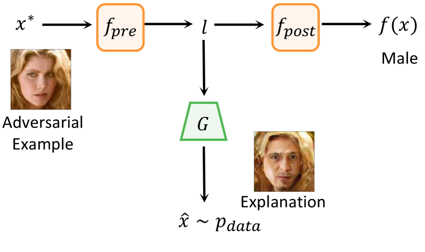
Figure 1: The network $G$ generates explanations $\hat{x}$ based on features relevant to classification in latent variable $l$, and $\hat{x}$ follows data distribution $p_{data}$.

Figure 2: Training framework of InterpretGAN. Compression network $C$ can reduce the dimension of latent variables. $L_{I}(G)$ is the interpretability term.

Since we use GAN to train network $G$, the generated explanations naturally satisfy the first property [18]. For the second property, we add an interpretability term in the min-max game of GAN (Eq. 2). The objective of the interpretability term is for the generated explanation $\hat{x}$ to contain a high mutual information with the classification result $f(x)$, which is $I(\hat{x},f(x))$. The higher the value of $I(\hat{x},f(x))$, the more information used for classification is contained in $\hat{x}$.

Therefore, to train InterpretGAN, we formalize the min-max game for our GAN training as the following, including a mutual information term as compared to equation 1:

$$\begin{split}\min_{G}\max_{D}V_{I}(D,G)&=V(D,G)-\lambda I(\hat{x},f(x))\\ &=V(D,G)-\lambda I(G(l),f(x)),\\ \text{where}\ V(D,G)&=\mathbb{E}_{x\sim p_{data}}[\log D(x)]+\mathbb{E}_{l\sim p_{l}}[\log(1-D(G(l)))].\end{split}$$ (2)

The calculation of the interpretability term $I(G(l),f(x))$ is intractable during training, but we can maximize the variational lower bound for $I(G(l),f(x))$ as a surrogate:

$$\begin{split}I(G(l),f(x))&=I(\hat{x},y)=H(y)-H(y|\hat{x})\\ &\geq\int_{\hat{x}}p(\hat{x})\int_{y}p(y|\hat{x})\log{p(\hat{y}|\hat{x})}dyd\hat{x}+H(y)\\ &=\mathbf{E}_{\hat{x}\sim G(l),y\sim f(x)}[\log{p(\hat{y}|\hat{x})}]+H(y)\triangleq L_{I}(G),\end{split}$$ (3)

where $y$ is $f(x)$, and $\hat{y}$ is $f(\hat{x})$. So the final optimization problem becomes:

$$\min_{G}\max_{D}V_{I}(D,G)=V(D,G)-\lambda L_{I}(G).$$ (4)

The training framework of our model is illustrated in Figure 2. In practice, since some latent variables have a large dimension, we adopt an extra compression network $C$ between the latent variables and the generative model. $C$ compresses the latent variables and controls the dimension of input for the generative model, which causes GAN training converge more efficiently.

In the following two sections, we divide our evaluation into two parts. In Section 4, InterpretGAN is used to explain how models classify natural images and adversarial images, and how adversarial perturbations lead to misclassification. In Section 5, a diagnostic method is designed based on InterpretGAN to quantify the vulnerability of each layer in a model.

4 Visual Explanation of Latent Variables for Classification

In this section, we apply our method to interpret classification models trained with two datasets: MNIST [13] and CelebFaces  [14] with gender as the label. For MNIST, we resize all images to $32\times 32$ for the convenience of GAN training and use a widely used model architecture in adversarial training research [6, 7, 17, 22, 9]. We use VGG$16$ [23] for the CelebFaces classification, and the generative models are trained with progressive GAN [24]. For MNIST, we interpret outputs for all convolutional and fully connected layers. For CelebFaces, we interpret outputs of all convolutional blocks and fully connected layers.

The results of interpreting the classification process of natural images and adversarial examples for the naturally trained models are presented in Section 4.1. Due to space limits, additional explanation results and detailed experiment configuration can be found in the supplementary material.

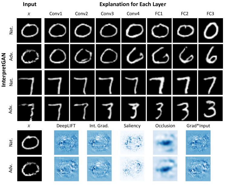
Figure 3: Explanations of classifications on natural images and corresponding adversarial images on the MNIST dataset. Explanations of adversarial examples are changed gradually through layers. Other interpretability methods can show the importance of pixels for classification of the natural image, but the explanation for the adversarial examples can’t explain the reason behind misclassification.

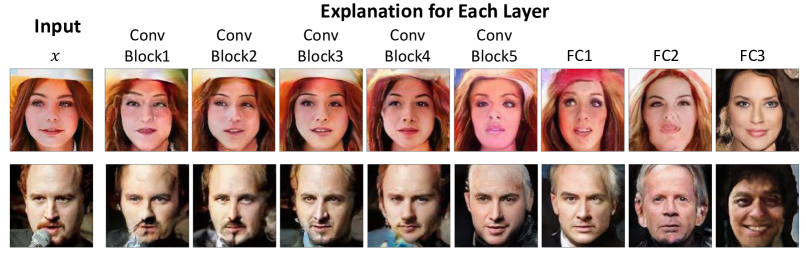
Figure 4: Generated explanations with features irrelevant to gender classification. The woman’s hat in the first row is transformed into her hair during classification. The microphone in the second row is filtered in the first two convolutional blocks and the blocked face is completed by the model.

4.1 Interpreting Classification Process

We interpret two models naturally trained with MNIST and CelebFaces datasets and compare the explanation results of our method to other interpretability methods (DeepLIFT [25], saliency maps [26], input$\times$gradient [27], integrated gradient [28], and occlusion [29]), which explain the relation between classification results and features. To investigate how adversarial perturbations influence features in the MNIST dataset, we use PGD-$40$ ($l_{\infty},\epsilon=0.3$) [30] and PGD-$20$ ($l_{\infty},\epsilon=2/255$) untargeted attacks to generate adversarial examples for MNIST and CelebFaces models. Figures 3 and 5 show the generated explanations for MNIST model and CelebFaces model, respectively.

Classification of Natural Images. The first and third rows in Figures 3 and  5 present the explanations of natural image classification. Since the generated explanations are regularized with the interpretability term in Eq. 2, we find that the explanations for natural images are consistent with the classification results, but not identical to the inputs. It is also observed that the model tries to only keep necessary features used for classification and tends to drop irrelevant features in latent variables. As shown in Figure 4, for a woman with a hat and a man with a microphone, the irrelevant features (hat and microphone) are gradually removed or transformed layer by layer.

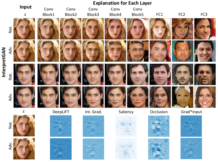
Figure 5: Explanations generated by our method and other baseline methods. InterpretGAN can illustrate which features are modified by adversarial perturbations. In shallower layers, local facial features are modified and, in deeper layers, backgrounds and hair are modified. Other interpretability methods have similar results to explanations on the MNIST dataset.

Classification of Adversarial Examples. When we feed adversarial examples into the models, the explanations are quite different. The second and fourth rows in Figures 3 and 5 show the explanations for corresponding adversarial examples. One interesting finding we notice for both models is that, rather than changing features directly in adversarial examples, adversarial perturbations influence latent variables gradually layer by layer: the deeper the layer is, the closer the explanation is to the misclassified label. However, we cannot find such difference in explanations generated by other baseline methods. We also find that adversarial perturbations influence features in latent variables in different ways for the MNIST and CelebFaces models.

For the MNIST model, although adversarial perturbations only change pixel values in the input images, explanations show that perturbations actually also modify features related to pixel position in latent variables. Figure 3 shows that the process of misclassification of adversarial "$0$" and "$7$". In addition to pixel values, pixel positions are also gradually changed so that perturbations can reuse these pixels to form new features for misclassified labels. The explanation "$6$" for adversarial "$0$" reuses most parts of original "$0$", and the explanation "$3$" for adversarial "$7$" is the curved version of the original "$7$".

When we perform the untargeted attack on MNIST, we find that adversarial examples with the same ground truth label are more likely to be misclassified as a certain label. For example, with the untargeted attack, $39.3\%$ adversarial "$0$"s are misclassified as "$6$", and $39.5\%$ adversarial "$7$"s are misclassified as "$3$". We think the reason is that it is easier for perturbations to spatially move original pixels to form features for the misclassified labels compared to only changing pixels values.

The CelebFaces dataset shows that adversarial perturbations influence different types of features in different layers: local features (e.g., nose, eyes, mouth, and beard) are more likely to be changed in shallower layers, and global features (e.g., hair and background) tend to be changed in deeper layers. As shown in Figure 5, when an adversarial "female" is fed into the model, the perturbations change eyes and nose first and then add a beard to the face. At a latter stage, the long blond hair is changed to short black hair. For the adversarial examples in the fourth line, eyes, lip, and make-up are changed in the shallower layers. Hair becomes longer in the explanations of Conv Block4 and Conv Block5.

5 Diagnosing Model Architecture

A crucial need for interpretability methods is how to take advantage of interpretability results to improve model performance [15]. What we have presented so far provides visual explanations for adversarial attacks, but not a diagnostic procedure to improve the model. In this section, we design a novel diagnostic method that can quantify the vulnerability contributed by each layer to adversarial attacks. We accomplish that by feeding the generated explanations back into the classification model and developing a metric to measure vulnerability contributed by each layer, as outlined next.

5.1 Quantifying Vulnerability for Layers

For a layer whose output is latent variable $l$ (i.e. , $l=f_{pre}(x)$, $f=f_{post}\circ f_{pre}$) and its generated explanation $\hat{x}=G(C(f_{pre}(x)))$, since features of $\hat{x}$ are only influenced by perturbations related to $f_{pre}$ and $\hat{x}$ follows the natural data distribution $p_{data}$, perturbations related to $f_{post}$ are filtered out in $\hat{x}$. If we feed $\hat{x}$ back to the classification model $f$, we can measure how much adversarial perturbations related to $f_{pre}$ change the classification result.

To evaluate the vulnerability of each layer against an adversarial dataset $\mathcal{D^{*}}$, we calculate the accuracy $Acc_{i}$ of the generated explanation $\hat{x}$ for the $i$th layer and introduce a metric defined as follows: the vulnerability ${Vul}_{i}$ of the $i$th layer is the accuracy drop as compared to the previous layer. Mathematically, it is formulated as:

$$\begin{split}Vul_{i}&=\begin{cases}1-Acc_{i}&i=1\\ Acc_{i-1}-Acc_{i}&i>1\end{cases}\\ Acc_{i}&=\mathbb{E}_{(x^{*},y)\in D^{*}}[\mathbf{1}_{\{true\}}(f(\hat{x_{i}})=y)]\\ \hat{x}_{i}&=G(C(f_{pre_{i}}(x^{*}))),\end{split}$$ (5)

where $\mathbf{1}$ is the indicator function, and $f_{{pre}_{i}}$ is the composition of layers until the $i$th layer.

5.2 Example: Diagnosis of MNIST Models

Layers		Conv1	Conv2	Conv3	Conv4	FC1	FC2	FC3
Naturally Trained	$Acc_{i}$	$52.6\%$	$26.3\%$	$21.6\%$	$9.9\%$	$4.3\%$	$3.0\%$	$3.5\%$
	$Vul_{i}$	$47.4\%$	$26.3\%$	$4.7\%$	$11.7\%$	$5.6\%$	$1.3\%$	$-0.5\%$
Adversarially Trained	$Acc_{i}$	$95.1\%$	$94.0\%$	$93.9\%$	$92.6\%$	$90.1\%$	$90.0\%$	$89.5\%$
	$Vul_{i}$	$4.9\%$	$1.1\%$	$0.1\%$	$1.3\%$	$2.5\%$	$0.1\%$	$0.5\%$

Table 1: Accuracy on InterpretGAN-generated images and the vulnerability of each layer for naturally- and adversarially-trained MNIST models. Red numbers indicate large accuracy drop (vulnerability).

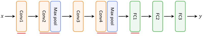
Figure 6: Architecture of the model used for MNIST classification. Red lines indicate layers with large accuracy drop (vulnerability) on generated images.

We use the proposed method to quantify the vulnerability of MNIST model architecture used in Section 4 and then quantify the vulnerability for a naturally trained model and an adversarially trained model. We perform PGD-$40$ $l_{\infty}$($\epsilon=0.3$) attack on a test set to obtain $D^{*}$, and we use ATTA-$1$ [9] to adversarially train the models.

Table 1 shows the diagnostic results. For both models, accuracy drops in almost all layers, which is consistent to our finding that perturbations influence latent variables gradually through layers. Specifically, we find that four layers (Conv1, Conv2, Conv4, and FC1) are more vulnerable than other layers. To study the reason behind these vulnerable layers, we locate them in the model architecture shown in Figure 6. For Conv1 (Conv layer after image) and FC1 (FC layer after Conv layer), we think the reason behind high vulnerability is that these two layers change the format of latent variables, which causes a higher information loss. Conv2 and Conv4 contain max pooling layers that down-sample latent features. The pooling layers in the MNIST model use $2\times 2$ filter and $2\times 2$ stride, which drops $75\%$ of latent variables during classification. The higher information loss can be the cause for the vulnerability of these layers. We compare the difference of max pooling indices (positions of the maximum value) between natural images and adversarial examples and find that, with PGD-$40$ ($l_{\infty},\epsilon=0.3$) attack, $40.9\%$ and $18.1\%$ max pooling indices change in the first and second pooling layers, respectively, which means that some important features in maximum variables used for natural classification are dropped. Besides changing the value of features, adversarial perturbations also drop important features in max pooling layers, likely leading to higher vulnerability of these layers.

	PGD-$40$	PGD-$100$	M-PGD-$40$	FGSM
Max Pooling	$89.33\%$	$81.98\%$	$89.76\%$	$95.62\%$
Avg Pooling	$91.56\%$	$87.48\%$	$92.09\%$	$95.72\%$

Table 2: Comparison of robustness between max pooling model and average pooling model on the MNIST. Model with average pooling layers show better robustness.

		PGD-$20$	PGD-$100$	M-PGD-$20$	FGSM
VGG16	Max Pooling	$46.97\%$	$45.69\%$	$47.06\%$	$50.46\%$
	Avg Pooling	$48.25\%$	$47.09\%$	$48.91\%$	$51.64\%$
WideResNet	Max pooling	$53.08\%$	$51.65\%$	$53.94\%$	$57.63\%$
	Avg pooling	$54.68\%$	$52.59\%$	$55.47\%$	$59.92\%$

Table 3: With average pooling layers, CIFAR10 models show better robustness under different adversarial attacks.

To mitigate the information loss in the max pooling layer, we propose using average pooling instead of max pooling. Compared to max pooling, average pooling uses all features to calculate outputs, which can retain more information during down-sampling. We adversarially retrain the MNIST model with average pooling layers and present a comparison of robustness under different attacks in Table 2. The results show that model robustness can be improved by simply replacing the max pooling layer with the average pooling layer. We also evaluate this experiment on the CIFAR10 dataset with VGG16 [23] and WideResNet [31]. The evaluation results shown in Table 3 also indicate that the average pooling layer tends to be more robust than the max pooling layer in these networks.

6 Related Work

Interpretability methods. Lots of efforts have tried understanding how DNNs classify images. Some works [32] study the relation between classification results and input features and most of the works [27, 28, 29] focus on estimating the importance (e.g., Shapley Value) of pixels in images. Others [20, 21, 33] also try to invert latent features back to the image space, but unlike our work, which generates explanation only based on relevant features used for classification, these works focus on reconstructing complete input images from all features encoded in latent variables. Similar to our work, there are also some recent research [34, 35, 36] designing interpretability methods based on generative models. The generative models generate explanations to determine which features need to be changed in input to change the confidence of classification. Singla et al. [34] also uses this method to generate saliency maps for input images. Unlike our work, none of the previous works study how adversarial perturbations influence features in latent variables.

Insights for building robust models. The reasons behind the existence of adversarial examples and how to build more robust models are still open questions. Goodfellow et al. [37, 38] suggested the cause of adversarial examples is the linear nature of layers in neural networks with sufficient dimensionality. Ilyas et al. [10] found that neural networks tend to use non-robust features for classification rather than robust features. Other works [39, 40] studied why adversarially trained models are more robust than naturally trained models. Xu et al. [11] applied network dissection [12] to interpret adversarial examples. Unlike previous research, in this work, we interpret adversarial examples from a new perspective, which produce additional insights for researchers to understand adversarial attacks.

7 Conclusion

In this work, we propose a novel interpretability method, as well as the first diagnostic method that can quantify the vulnerability contributed by each layer against adversarial attacks. By factoring in the mutual information between generated images and classification results, InterpretGAN generates explanations containing relevant features used for classification in latent variables at each layer. The generated explanations show how and what features are influenced by adversarial perturbations. We also propose a new vulnerability metric that can be computed using InterpretGAN to provide insights to identify vulnerable parts of models against adversarial attacks. Based on the diagnostic results, we study the relationship between robustness and model architectures. Specifically, we find that, to design a robust model, average pooling layers can be a more reliable than max pooling layers.

Acknowledgement. This material is based on work supported by DARPA under agreement number 885000, the National Science Foundation (NSF) Grants 1646392, and Michigan Institute of Data Science (MIDAS). We also thank researchers at Ford for their feedback on this work and support from Ford to the University of Michigan.

Appendix A Overview

This supplementary material provides detailed configuration information of our derivation and experiments. Section B includes a detailed derivation process of the variational lower bound for the mutual information. Section C describes the detailed model architecture and experimental setup. Section D presents additional examples of explanations.

Appendix B Derivation of Variational Lower Bound of Interpretability Term

The derivation for Equation 3 of the paper is shown below in further detail.

To show (Eq. 3):

$$\begin{split}I(G(l),f(x))&=I(\hat{x},y)=H(y)-H(y|\hat{x})\\ &\geq\int_{\hat{x}}p(\hat{x})\int_{y}p(y|\hat{x})\log{p(\hat{y}|\hat{x})}dyd\hat{x}+H(y)\\ &=\mathbf{E}_{\hat{x}\sim G(l),y\sim f(x)}[\log{p(\hat{y}|\hat{x})}]+H(y)\triangleq L_{I}(G)\end{split}$$

Derivation:

$$\begin{split}I(G(l),f(x))&=I(\hat{x},y)=H(y)-H(y|\hat{x})\\ &=\int_{\hat{x}}\int_{y}p(y,\hat{x})\log p(y|\hat{x})dyd\hat{x}+H(y)\\ &=\int_{\hat{x}}p(\hat{x})\int_{y}p(y|\hat{x})\log p(y|\hat{x})dyd\hat{x}+H(y)\\ &=\int_{\hat{x}}p(\hat{x})\int_{y}(p(y|\hat{x})\log\frac{p(y|\hat{x})}{p(\hat{y}|\hat{x})}+p(y|\hat{x})\log{p(\hat{y}|\hat{x})})dyd\hat{x}+H(y)\\ &=\int_{\hat{x}}p(\hat{x})\int_{y}(D_{KL}(p(y|\hat{x})||p(\hat{y}|\hat{x}))+p(y|\hat{x})\log{p(\hat{y}|\hat{x})})dyd\hat{x}+H(y)\\ &\geq\int_{\hat{x}}p(\hat{x})\int_{y}p(y|\hat{x})\log{p(\hat{y}|\hat{x})}dyd\hat{x}+H(y)\\ &=\int_{\hat{x}}\int_{y}p(y,\hat{x})\log{p(\hat{y}|\hat{x})}dyd\hat{x}+H(y)\\ &=\mathbf{E}_{\hat{x}\sim G(l),y\sim f(x)}[\log{p(\hat{y}|\hat{x})}]+H(y)\triangleq L_{I}(G),\end{split}$$

where $D_{KL}$ is the Kullback–Leibler divergence and $H(x)$ is the entropy of random variable $x$.

Appendix C Model Architecture and Experiment Setup

In this section, we provide additional details on the implementation, model architecture, and hyper-parameters used in this work. For the baseline methods used in Section 4, we use Captum [41] to generate explanations.

Classification models. For the MNIST dataset, we use the same model architecture as used in [6, 7, 22], which has four convolutional layers and three fully-connected layers. The naturally trained model is trained for $10$ epochs with a $0.01$ learning rate in the first $5$ epochs and a $0.001$ learning rate in the last $5$ epochs. For the CelebFaces dataset, we use VGG$16$ [23] for gender classification. The naturally trained model is trained for $7$ epochs with a $0.001$ learning rate. In Section 5, for the CIFAR10 dataset, we use VGG$16$ [23] and Wide-Resnet-34-10 [31] as the model architecture.

Adversarial attack and adversarial training. For generating adversarial examples, we perform PGD-$40$ ($l_{\infty},\epsilon=0.3$) [30] attack on the MNIST dataset, PGD-$20$ ($l_{\infty},\epsilon=2/255$) attack on the CelebFaces dataset, and PGD-$20$ ($l_{\infty},\epsilon=8/255$) attack on the CIFAR10 dataset. For adversarial training used in Section 5, we use ATTA-$1$ [9] with TRADES loss ($\beta=6$)[7] (and with recommended hyperparameters from  [7]) to train the model.

Generative models. We use progressive GAN [24] to train the generative models for the MNIST [13] and the CelebFaces [14] datasets. For latent variables in different layers, we use the same architecture for explanation generators. Different compression networks were used to connect latent variables and explanation generators, as described in Tables 4 and 5 for MNIST and CelebFaces, respectively. We set $\lambda=1$ for all InterpretGAN training.

For the explanation generators of the MNIST dataset, we resize the image to $32$ for the convenience of progressive GAN training. Explanation generators have $4$ scales, and each scale has $2$ convolutional layers and are connected with an up-sample layer. The outputs of each scale are $4\times 4$, $8\times 8$, $16\times 16$, and $32\times 32$. The discriminators have an inversed architecture, but up-sample layers are replaced by down-sample layers. For the first three scales, each scale is trained for $6$ epochs, and the last (fourth) scale is trained for another $12$ epochs. All epochs use a $0.001$ learning rate. Our implementation of progressive GAN for MNIST is based on https://github.com/jeromerony/Progressive_Growing_of_GANs-PyTorch.

For the explanation generators of the CelebFaces dataset, as in progressive GAN [24], we resize the image to $128\times 128$. Explanation generators have $6$ scales, and each scale has $2$ convolutional layers and is connected with an up-sample layer. The outputs of each scale are $4\times 4$, $8\times 8$, $16\times 16$, $32\times 32$, $64\times 64$, and $128\times 128$. The discriminators have an inversed architecture but with up-sample layers replaced by down-sample layers. Our implementation of progressive GAN is based on https://github.com/facebookresearch/pytorch_GAN_zoo. The first scale is trained for $48,000$ iterations. For the other $5$ scales, each scale is trained for $96,000$ iterations.

Layers	Compression Network Architecture
Conv1	$3\times 3$ Conv, $64$ $\to$ AvgPooling $\to$ $3\times 3$ Conv, $128$ $\to$ AvgPooling $\to$ $3\times 3$ Conv, $256$ $\to$ AvgPooling $\to$ FC
Conv2	$3\times 3$ Conv, $64$ $\to$ AvgPooling $\to$ $3\times 3$ Conv, $128$ $\to$ AvgPooling $\to$ FC
Conv3	$3\times 3$ Conv, $128$ $\to$ AvgPooling $\to$ $3\times 3$ Conv, $256$ $\to$ AvgPooling $\to$ FC
Conv4	FC
FC1	FC
FC2	FC
FC3	FC

Table 4: Compression network archtectures for different layers of the MNIST model.

Layers	Compression Network Architecture
Conv Block1	$3\times 3$ Conv, $128$ $\to$ AvgPooling $\to$ $3\times 3$ Conv, $256$ $\to$ AvgPooling $\to$ $3\times 3$ Conv, $512$ $\to$ AvgPooling $\to$ $3\times 3$ Conv, $512$ $\to$ AvgPooling
Conv Block2	$3\times 3$ Conv, $256$ $\to$ AvgPooling $\to$ $3\times 3$ Conv, $512$ $\to$ AvgPooling $\to$ $3\times 3$ Conv, $512$ $\to$ AvgPooling
Conv Block3	$3\times 3$ Conv, $512$ $\to$ AvgPooling $\to$ $3\times 3$ Conv, $512$ $\to$ AvgPooling
Conv Block4	$3\times 3$ Conv, $512$ $\to$ AvgPooling
Conv Block5	$3\times 3$ Conv, $512$
FC1	FC
FC2	FC
FC3	FC

Table 5: Compression network archtectures for different layers of the CelebFaces model.

Appendix D Additional Experiment Results

In this section, we present additional examples and results for Section 4 in the paper. Figure 7 shows the distribution of misclassified labels of the MNIST dataset under an untargeted attack. As discussed in Section 4.1 in the paper, we find that, under an untargeted attack, images with different ground truth labels tend to be misclassified as different labels. A possible reason is that, given an image with a ground truth label, it is easier for perturbations to change the image to a similar image with a misclassified label by changing the position features of some pixels, while reusing some of the original pixels. We also present more explanation examples of classification on natural images and adversarial images in Figures 4, 8, 9, and 11.

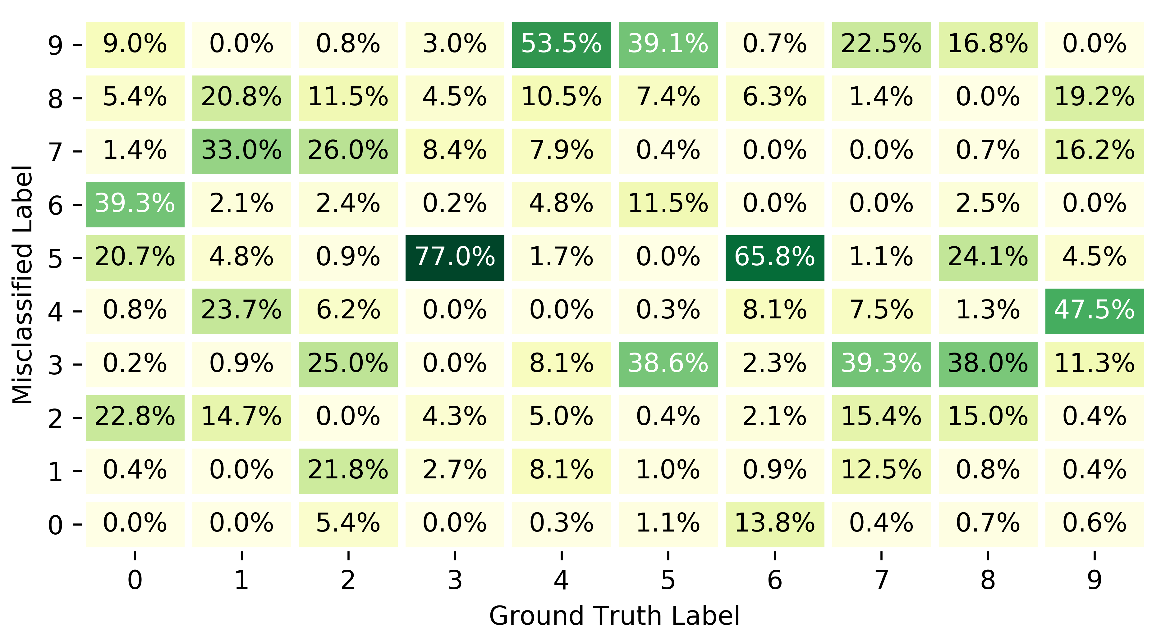
Figure 7: The distribution of misclassified labels: the different ground truth labels tend to be misclassified as different labels.

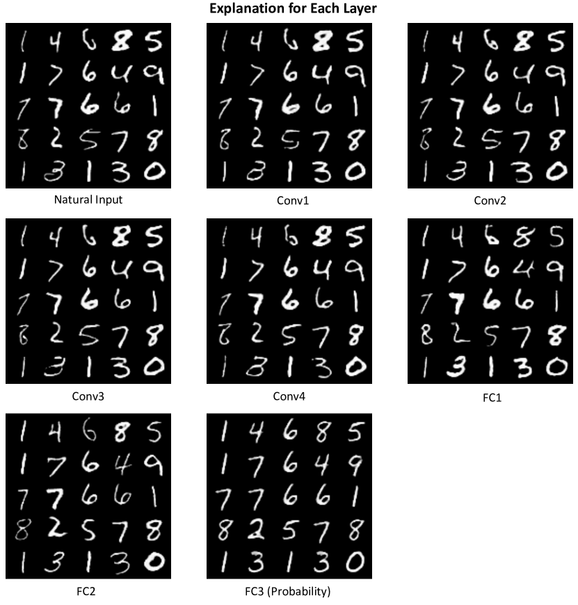
Figure 8: Explanations for randomly selected natural images from the test dataset.

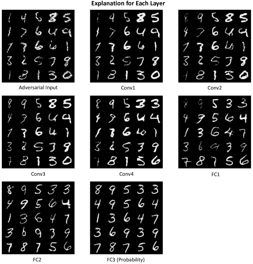
Figure 9: Explanations for adversarial images generated by PGD-$40$ for images in Figure 8.

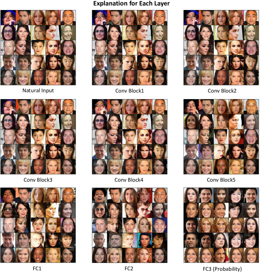
Figure 10: Explanations for randomly selected natural images from the test dataset.

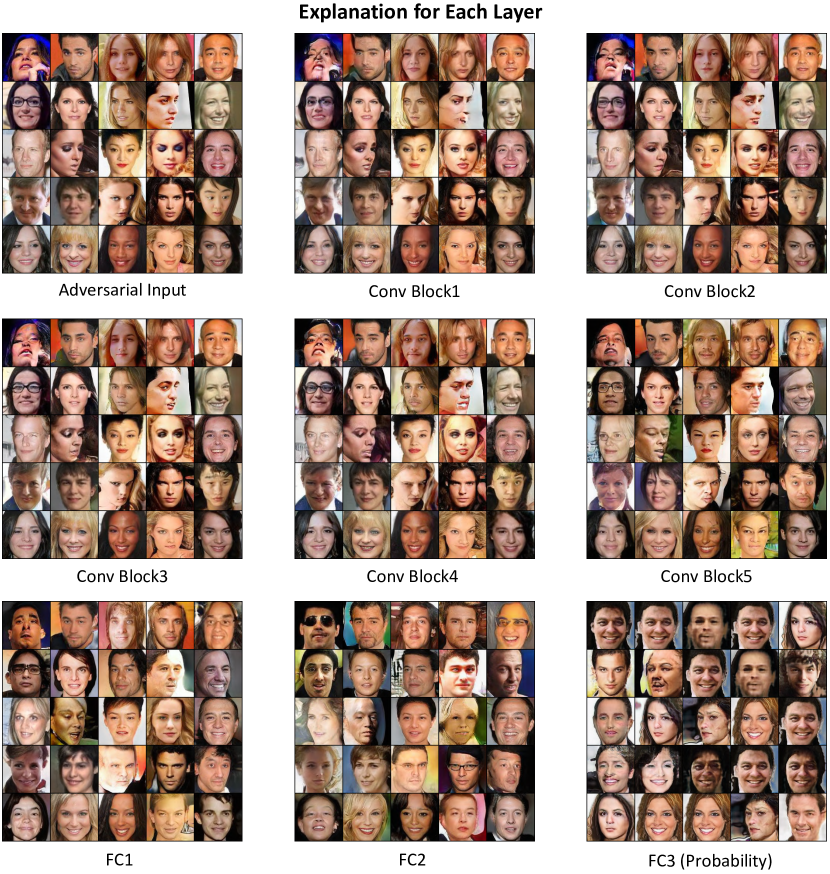
Figure 11: Explanations for adversarial images generated by PGD-$40$ for images in Figure 10.

References

- [1] Szegedy, C., W. Zaremba, I. Sutskever, et al. Intriguing properties of neural networks. In International Conference on Learning Representations (ICLR). 2014.
- [2] Cohen, J. M., E. Rosenfeld, J. Z. Kolter. Certified adversarial robustness via randomized smoothing. In International Conference on Machine Learning (ICML). 2019.
- [3] Raghunathan, A., J. Steinhardt, P. Liang. Certified defenses against adversarial examples. In International Conference on Learning Representations (ICLR). 2018.
- [4] Hein, M., M. Andriushchenko. Formal guarantees on the robustness of a classifier against adversarial manipulation. In Advances in Neural Information Processing Systems (NeurIPS), pages 2266–2276. 2017.
- [5] Wong, E., J. Z. Kolter. Provable defenses against adversarial examples via the convex outer adversarial polytope. In International Conference on Machine Learning (ICML). 2018.
- [6] Madry, A., A. Makelov, L. Schmidt, et al. Towards deep learning models resistant to adversarial attacks. In International Conference on Learning Representations (ICLR). 2018.
- [7] Zhang, H., Y. Yu, J. Jiao, et al. Theoretically principled trade-off between robustness and accuracy. In International Conference on Machine Learning (ICML). 2019.
- [8] Tramèr, F., A. Kurakin, N. Papernot, et al. Ensemble adversarial training: Attacks and defenses. In International Conference on Learning Representations (ICLR). 2018.
- [9] Zheng, H., Z. Zhang, J. Gu, et al. Efficient adversarial training with transferable adversarial examples. arXiv preprint arXiv:1912.11969, 2019.
- [10] Ilyas, A., S. Santurkar, D. Tsipras, et al. Adversarial examples are not bugs, they are features. arXiv preprint arXiv:1905.02175, 2019.
- [11] Xu, K., S. Liu, G. Zhang, et al. Interpreting adversarial examples by activation promotion and suppression. arXiv preprint arXiv:1904.02057, 2019.
- [12] Bau, D., B. Zhou, A. Khosla, et al. Network dissection: Quantifying interpretability of deep visual representations. In Proceedings of the IEEE Conference on Computer Vision and Pattern Recognition (CVPR), pages 6541–6549. 2017.
- [13] LeCun, Y., L. Bottou, Y. Bengio, et al. Gradient-based learning applied to document recognition. Proceedings of the IEEE, 86(11):2278–2324, 1998.
- [14] Liu, Z., P. Luo, X. Wang, et al. Deep learning face attributes in the wild. In Proceedings of International Conference on Computer Vision (ICCV). 2015.
- [15] Bhatt, U., A. Xiang, S. Sharma, et al. Explainable machine learning in deployment. In Proceedings of the 2020 Conference on Fairness, Accountability, and Transparency, pages 648–657. 2020.
- [16] Krizhevsky, A., G. Hinton, et al. Learning multiple layers of features from tiny images. Tech. rep., Citeseer, 2009.
- [17] Shafahi, A., M. Najibi, A. Ghiasi, et al. Adversarial training for free! In Advances in Neural Information Processing Systems (NeurIPS). 2019.
- [18] Goodfellow, I., J. Pouget-Abadie, M. Mirza, et al. Generative adversarial nets. In Advances in Neural Information Processing Systems (NeurIPS), pages 2672–2680. 2014.
- [19] Chen, X., Y. Duan, R. Houthooft, et al. Infogan: Interpretable representation learning by information maximizing generative adversarial nets. In Advances in Neural Information Processing Systems (NeurIPS), pages 2172–2180. 2016.
- [20] Mahendran, A., A. Vedaldi. Understanding deep image representations by inverting them. In Proceedings of the IEEE Conference on Computer Vision and Pattern Recognition (CVPR), pages 5188–5196. 2015.
- [21] Dosovitskiy, A., T. Brox. Inverting visual representations with convolutional networks. In PProceedings of the IEEE Conference on Computer Vision and Pattern Recognition (CVPR), pages 4829–4837. 2016.
- [22] Zhang, D., T. Zhang, Y. Lu, et al. You only propagate once: Accelerating adversarial training via maximal principle. In Advances in Neural Information Processing Systems (NeurIPS). 2019.
- [23] Simonyan, K., A. Zisserman. Very deep convolutional networks for large-scale image recognition. In International Conference on Learning Representations (ICLR). 2014.
- [24] Karras, T., T. Aila, S. Laine, et al. Progressive growing of gans for improved quality, stability, and variation. In International Conference on Learning Representations (ICLR). 2018.
- [25] Shrikumar, A., P. Greenside, A. Kundaje. Learning important features through propagating activation differences. In International Conference on Machine Learning (ICML), pages 3145–3153. JMLR. org, 2017.
- [26] Simonyan, K., A. Vedaldi, A. Zisserman. Deep inside convolutional networks: Visualising image classification models and saliency maps. In International Conference on Learning Representations (ICLR). 2014.
- [27] Kindermans, P.-J., K. Schütt, K.-R. Müller, et al. Investigating the influence of noise and distractors on the interpretation of neural networks. In Advances in Neural Information Processing Systems (NeurIPS). 2016.
- [28] Sundararajan, M., A. Taly, Q. Yan. Axiomatic attribution for deep networks. In International Conference on Machine Learning (ICML), pages 3319–3328. 2017.
- [29] Zeiler, M. D., R. Fergus. Visualizing and understanding convolutional networks. In Proceedings of the European Conference on Computer Vision (ECCV), pages 818–833. 2014.
- [30] Kurakin, A., I. Goodfellow, S. Bengio. Adversarial machine learning at scale. In International Conference on Learning Representations (ICLR). 2017.
- [31] Zagoruyko, S., N. Komodakis. Wide residual networks. arXiv preprint arXiv:1605.07146, 2016.
- [32] Ribeiro, M. T., S. Singh, C. Guestrin. " why should i trust you?" explaining the predictions of any classifier. In Proceedings of the 22nd ACM SIGKDD international conference on knowledge discovery and data mining, pages 1135–1144. 2016.
- [33] Selvaraju, R. R., M. Cogswell, A. Das, et al. Grad-cam: Visual explanations from deep networks via gradient-based localization. In Proceedings of International Conference on Computer Vision (ICCV), pages 618–626. 2017.
- [34] Singla, S., B. Pollack, J. Chen, et al. Explanation by progressive exaggeration. In International Conference on Learning Representations (ICLR). 2020.
- [35] Samangouei, P., A. Saeedi, L. Nakagawa, et al. Explaingan: Model explanation via decision boundary crossing transformations. In Proceedings of the European Conference on Computer Vision (ECCV), pages 666–681. 2018.
- [36] Dosovitskiy, A., T. Brox. Generating images with perceptual similarity metrics based on deep networks. In Advances in Neural Information Processing Systems (NeurIPS), pages 658–666. 2016.
- [37] Goodfellow, I. J., J. Shlens, C. Szegedy. Explaining and harnessing adversarial examples. In International Conference on Learning Representations (ICLR). 2014.
- [38] Zhou, B., A. Khosla, A. Lapedriza, et al. Learning deep features for discriminative localization. In Proceedings of the IEEE Conference on Computer Vision and Pattern Recognition (CVPR), pages 2921–2929. 2016.
- [39] Zhang, T., Z. Zhu. Interpreting adversarially trained convolutional neural networks. In International Conference on Machine Learning (ICML). 2019.
- [40] Etmann, C., S. Lunz, P. Maass, et al. On the connection between adversarial robustness and saliency map interpretability. In International Conference on Machine Learning (ICML). 2019.
- [41] Kokhlikyan, N., V. Miglani, M. Martin, et al. Pytorch captum. https://github.com/pytorch/captum, 2019.