Integration of Survival Data from Multiple Studies

Abstract

We introduce a statistical procedure that integrates survival data from multiple biomedical studies, to improve the accuracy of predictions of survival or other events, based on individual clinical and genomic profiles, compared to models developed leveraging only a single study or meta-analytic methods. The method accounts for potential differences in the relation between predictors and outcomes across studies, due to distinct patient populations, treatments and technologies to measure outcomes and biomarkers. These differences are modeled explicitly with study-specific parameters. We use hierarchical regularization to shrink the study-specific parameters towards each other and to borrow information across studies. Shrinkage of the study-specific parameters is controlled by a similarity matrix, which summarizes differences and similarities of the relations between covariates and outcomes across studies. We illustrate the method in a simulation study and using a collection of gene-expression datasets in ovarian cancer. We show that the proposed model increases the accuracy of survival prediction compared to alternative meta-analytic methods.
Keywords: Meta-Analysis, Survival Analysis, Risk Prediction, Hierarchical Regularization.

1 Introduction

Various biomedical technologies enable the use of omics information for prognostic purposes, to quantify the risk of diseases, or to predict response to treatments. Risk stratification in oncology often utilizes a set of biomarkers to predict cancer progression or death within a time period. The number of covariates can exceed the sample size. This makes the identification of relevant genomic features for risk prediction and the development of accurate models challenging. Penalized regression and methods that utilize multiple datasets have been discussed in this context. Penalization methods enable parameter estimation and prediction when the number of predictors is large [46]. Meta-analyses [16] and integrated analyses [12] combine information from multiple studies for parameter estimation and prediction [24, 48]. These statistical procedures improve the estimation of parameters of interest with respect to single-study estimates if the covariate-outcome relations are similar across studies [40, 3, 51]. For instance Riester et al. [40], Bernau et al. [3] and Waldron et al. [51] showed that meta-analytic procedures tend to outperform the prediction accuracy of models developed using only a single study. But [40, 51, 47] also described heterogeneity of covariate effects across cancer studies, due to differences in assays, treatments and patient populations.

We introduce a model for the integrated analysis of a collection of datasets, with the aim of improving the accuracy of predictions, compared to single-study models and meta-analytic procedures. We use study-specific parameters in covariate-outcome regression models. These parameters are estimated borrowing information across studies with hierarchical regularization, which shrinks the study-specific regression coefficients towards each other. We use a squared $K\times K$ similarity matrix representative of differences and similarities of the covariates’ effects across $K$ studies. The matrix is used to estimate the study-specific models. The regression parameters of each study are shrunken more towards the parameters of similar studies and less towards the remaining studies.

In previous work on integrative analyses Liu et al. [28] discussed Bayesian methods and variable selection for accelerated failure time models. Hierarchical normal models for multi-study gene expression analyses have been developed in [12, 11, 13], and Ma et al. [30, 31] studied penalized regression methods for integrative analyses, focusing on binary and accelerated failure-time outcome models. For case-control analyses with multiple datasets, Liu et al. [29] proposed an adaptive group-LASSO (agLASSO) procedure, and Cheng et al. [10] extended the approach using different regularization techniques. In the following sections we introduce a procedure which builds on the work that we mentioned. The procedure shrink study-specific parameters towards each other accounting for the degrees of similarity specific of each pair of studies.

2 The multi-study model

We consider $K$ studies with time-to-event outcomes and predictors such as gene expression measurements. For each study $k=1,\ldots,K$ the vector $\bm{Y}_{k}=\{Y_{k,i}\}_{i=1}^{n_{k}}$ indicates (possibly censored) survival times of $n_{k}$ individuals and $\bm{C}_{k}=\{C_{k,i}\}_{i=1}^{n_{k}}$ denotes the vector of censoring variables, where $C_{k,i}=1$ if $Y_{k,i}$ is an observed event time and it is zero if there is censoring at time $Y_{k,i}$. The vector $\bm{x}_{k,i}\in\mathbb{R}^{p}$ represents a set of $p$ predictors and $\bm{X}_{k}=(\bm{x}_{k,1},\cdots,\bm{x}_{k,n_{k}})^{T}$. Lastly, $\mathcal{D}_{k}=(\bm{Y}_{k},\bm{C}_{k},\bm{X}_{k})$ indicates the data from study $k$ and $\mathcal{D}=\{\mathcal{D}_{k}\}_{k=1}^{K}$ is a collection of studies.

We assume that failure times in each study $k$ follow a proportional hazard model [14] with baseline survival function $S_{k}(\cdot)$ and study-specific coefficients $\bm{\beta}_{k}\in\mathbb{R}^{p}.$ The approach that we will describe can be applied to alternative time to event models, for instance to accelerated failure time models [53] or accelerated hazards models [9], computations would only require minor modifications.

Inference is based on the Breslow’s modification of the partial log-likelihood functions [14] for (possible tied) survival times,

$$l\left(\bm{\beta}_{k},\mathcal{D}_{k}\right)=\sum_{\ell=1}^{m_{k}}\left\{\bm{\tilde{x}}^{\prime}_{k,\ell}\bm{\beta}_{k}-d_{k,\ell}\log\left(\sum_{i:Y_{k,i}\geq t_{k,\ell}}\exp\{\bm{x}_{k,i}^{\prime}\bm{\beta}_{k}\}\right)\right\},$$

where $\big{\{}t_{k,\ell}\big{\}}_{\ell=1}^{m_{k}}$ are the $m_{k}$ unique event times in study $k$, $d_{k,\ell}$ denotes the number of observed events at time $t_{k,\ell}$, $\displaystyle\bm{\tilde{x}}_{k,\ell}=\sum_{i}\bm{x}_{k,i}I(C_{k,i}=1,Y_{k,i}=t_{k,\ell}),$ for $\ell=1,\ldots,m_{k},$ and $I(A)$ is the indicator function of the event $A$.

When the number of predictors exceeds the number of observed events a unique maximum partial-likelihood estimate does not exist and maximization of the regularized likelihood function $l\left(\bm{\beta}_{k},\mathcal{D}_{k}\right)-R\left(\bm{\beta}_{k}\right)$ has been proposed [46, 34, 43] to obtain covariate effect estimates. Here $R\left(\bm{\beta}_{k}\right)$ is a non-negative function that equals zero when $\bm{\beta}_{k}=\bm{0}$. Popular approaches include the LASSO, ridge, elastic-net and the bridge penalties to name a few [25, 45, 46, 19, 52, 43]. We refer to [5, 6, 50, 3] for comparisons of regularization methods for predicting survival outcomes using genomic profiles.

As demonstrated in [3] studies, with nearly identical aims, often presents different joint distributions of predictors $\bm{x}_{k,i}$ and outcomes $Y_{k,i}$. Clusters of studies which correspond to different essays, patient populations, treatments, and study designs have been discussed [3, 47]. We introduce a model with study-specific parameters $\bm{\beta}_{k}$, and a latent parameter $\bm{\beta}_{0}$, which can be interpreted as the mean parameter across studies. Some studies will have similar vectors $\bm{\beta}_{k}$ due to similarities in the assays and patient populations, while other studies might be considerably different [3, 51]. We estimate the vectors $\bm{\beta}_{k}$ by borrowing information from studies $k^{\prime}\neq k$ that are similar to study $k$. At the same time, studies $k^{\prime}$ that differ substantially from study $k$ will have little influence on the estimation of $\bm{\beta}_{k}$. In different words, borrowing of information mirrors similarities and differences across studies. The latent parameter and study-level parameters $\bm{\beta}=(\bm{\beta}_{0},\cdots,\bm{\beta}_{K})$ are estimated using the regularized likelihood

$$l_{R}\left(\bm{\beta}\right)=\sum_{k=1}^{K}l\left(\bm{\beta}_{k},\mathcal{D}_{k}\right)-R_{0}(\bm{\beta}_{0})-R_{1}\left(\bm{\beta}\right).$$ (1)

Here the parameters $\bm{\beta}_{k}$ can be interpreted as a noisy realization of $\bm{\beta}_{0}$, the average effect across studies. The non-negative function $R_{0}(\cdot)$ regularizes $\bm{\beta}_{0}$ and is zero when $\bm{\beta}_{0}=\bm{0}$ (for example a lasso penalty). Similarly, the non-negative function $R_{1}(\cdot)$ is zero when $\bm{\beta}_{0}=\bm{\beta}_{1}=\cdots=\bm{\beta}_{K}$ (see below for examples) and is used to borrow information across studies in the estimation of $\bm{\beta}$. In our applications in Sections 4 and 5 we will use $\widehat{\bm{\beta}}_{0}$ for risk predictions of patients in populations $k>K$ that are not represented in our collection of $K$ studies, whereas for patients belonging to populations $k=1,\dots,K,$ the estimate $\widehat{\bm{\beta}}_{k}$ can be directly used for risk predictions.

Penalized maximum likelihood estimates based on (1) have a Bayesian interpretation. See [45, 23, 37, 35] for a discussion on the relations between regularization methods and Bayesian analyses. Consider a Bayesian model for the unknown parameters $\bm{\beta}$, with prior probability $Pr(\bm{\beta}_{0})\propto e^{-R_{0}(\bm{\beta}_{0})}$ for the vector $\bm{\beta}_{0}$ and $Pr(\bm{\beta}_{1},\dots,\bm{\beta}_{K}|\bm{\beta}_{0})\propto e^{-R_{1}\left(\bm{\beta}\right)}$ for the study specific parameters conditionally on $\bm{\beta}_{0}$. The approximate posterior density of $\bm{\beta}$ with respect to the partial likelihood (see [44] for a formal justification) is proportional to

$$Pr_{PL}\left(\bm{\beta}|\mathcal{D}\right) \propto Pr(\bm{\beta}_{0})Pr(\bm{\beta}_{1},\cdots,\bm{\beta}_{K}|\bm{\beta}_{0})\prod_{k=1}^{K}e^{l(\bm{\beta}_{k},\mathcal{D}_{k})}.$$ (2)

Therefore the mode of (2) coincides with the parameter $\bm{\beta}$ that maximizes (1). If we set $R_{1}\left(\bm{\beta}\right)=\sum_{k}\tilde{R}_{1}\left(\bm{\beta}_{k},\bm{\beta}_{0}\right)$, with $\tilde{R}_{1}\left(\bm{\beta}_{k},\bm{\beta}_{0}\right)\geq 0$ then the Bayesian model (2) incorporates the assumption that studies are exchangeable with, conditionally on $\bm{\beta}_{0}$, independent and identically distributed covariate effects $\bm{\beta}_{k}$. For example $\tilde{R}_{1}\left(\bm{\beta}_{k},\bm{\beta}_{0}\right)=||\bm{\beta}_{k}-\bm{\beta}_{0}||^{2}_{2}/(2\lambda_{1})$ and $R_{0}\left(\bm{\beta}_{0}\right)=||\bm{\beta}_{0}||_{2}^{2}/(2\lambda_{0})$ is consistent with the commonly utilized hierarchical normal prior model with, a priori, correlations $\mbox{Cor}(\beta_{k,j},\beta_{k^{\prime},j})=\lambda_{0}/(\lambda_{0}+\lambda_{1})>0$ for studies $k^{\prime}\neq k$ when the latent vector $\bm{\beta}_{0}$ is integrated out. This regularization implies positive and symmetric borrowing of information for all pairs $k\neq k^{\prime}$ of studies, and may not be appropriate for groups of studies with different patient populations.

For the latent mean parameter $\bm{\beta}_{0}$ we use the elastic-net penalty [54],

$$R_{0}(\bm{\beta}_{0})=\lambda_{0}||\bm{\beta}_{0}||_{1}+\lambda_{1}||\bm{\beta}_{0}||_{2}^{2},$$

$\lambda_{0},\lambda_{1}\geq 0,$ with LASSO and ridge penalty as special cases, when $\lambda_{1}=0$ and $\lambda_{0}=0$ respectively.

To account for differences and similarities of the available studies, we use

$$R_{1}\left(\bm{\beta}\right)=\sum_{j=1}^{p}||\bm{\beta}_{1:K,j}-\beta_{0,j}\bm{1}||_{\bm{\Sigma}}^{a}$$ (3)

in (1), where $\bm{1}$ is a K-dimensional vector with one on each component, $\bm{\beta}_{1:K,j}=(\beta_{1,j},\cdots,\beta_{K,j})^{\prime}$ refers to covariate $j=1,\cdots,p$ in each study, and $||\bm{x}||_{\bm{\Sigma}}=\sqrt{\bm{x}^{\prime}\bm{\Sigma}^{-1}\bm{x}}$. The symmetric matrix $\bm{\Sigma}$ is positive-semidefinite and enables differential borrowing of information across studies.

For $a=2$, the minimizer of (1) is equivalent to the posterior mode when, a priori, the coefficients $\bm{\beta}_{1:K,j},j=1,\cdots,p$ across studies are modeled as multivariate normal with mean $\beta_{0,j}\bm{1}$ and covariance matrix $\bm{\Sigma}$. In this case $\Sigma_{k,k^{\prime}}=0$ implies that $\bm{\beta}_{k}$ and $\bm{\beta}_{k^{\prime}}$ are, a priori and conditionally on $\bm{\beta}_{0}$ independent. Whereas a large covariance $\Sigma_{k,k^{\prime}}>0$ indicates similarities between $\bm{\beta}_{k}$ and $\bm{\beta}_{k^{\prime}}$.

For $a=1$ the penalty $R_{1}(\bm{\beta})$ in (3) becomes the sum of Mahalanobis distance of $\bm{\beta}_{1:K,j}$ from the mean $\beta_{0,j}\bm{1}$ with covariance matrix $\bm{\Sigma}$. With $\bm{\Sigma}\propto\bm{I}$ this penalty reduces to the group LASSO [10, 29] with one group for each covariate $j=1,\cdots,J$.

The regularization parameters $\lambda_{0},\lambda_{1},a,$ and $\bm{\Sigma}$ determine (i) the sparsity of $\widehat{\bm{\beta}}_{0}$ (the number of components $\widehat{\beta}_{0,j}=0$) and (ii) the similarity of the estimates $\widehat{\beta}_{1,j},\cdots,\widehat{\beta}_{K,j}$ across studies, including the number of identical study-specific estimates $\widehat{\beta}_{k,j}=\widehat{\beta}_{k^{\prime},j}$.

When $a\geq 1$, $\bm{\Sigma}$ is positive-definite and $\lambda_{0}>0$ or $\lambda_{1}>0$, the regularized log-partial-likelihood (1) is concave. If we fix $\lambda_{1}\geq 0,$ $a\geq 1$ and the positive-definite matrix $\bm{\Sigma},$ then the number of components $\widehat{\beta}_{0,j}$ equal to $0$ increases with $\lambda_{0}.$ For instance, consider $a>1$ in (1), $\lambda_{1}=0$, and $g(\bm{\beta}_{0})=\max_{\bm{\beta}_{1},\cdots,\bm{\beta}_{K}}\sum_{k=1}^{K}l\left(\bm{\beta}_{k},\mathcal{D}_{k}\right)-R_{1}\left(\bm{\beta}\right).$ The concave map $g(\bm{\beta}_{0})-\lambda_{0}||\bm{\beta}_{0}||_{1}$ bounds the regularized log-partial-likelihood. If we choose $\lambda_{0}$ larger than $\max_{1\leq j\leq p}|\partial g(\bm{\beta}_{0})/\partial\beta_{0,j}|$ at $\bm{\beta}_{0}=\bm{0}$, then (1) is maximized at $\widehat{\bm{\beta}_{0}}=\bm{0}$. In contrast, for values $\lambda_{0}$ below this maximum some of the estimates $\widehat{\beta}_{0,j}$ will be different from zero.

For $\lambda_{0},\lambda_{1}\geq 0,$ and $a=1$, the choice of $\bm{\Sigma}$ can lead to identical study specific estimates $\widehat{\beta}_{1,j}=\cdots=\widehat{\beta}_{K,j}$. We provide an example with $\lambda_{0}=0$ and $\bm{\Sigma}=\sigma^{2}\bm{I}$. Let $\bm{z}_{k}=\bm{\beta}_{k}-\bm{\beta}_{0},k=1,\cdots,K$, and define $h(\bm{z})=\max_{\bm{\beta}_{0}}\sum_{k=1}^{K}l\left(\bm{z}_{k}+\bm{\beta}_{0},\mathcal{D}_{k}\right)-R_{0}\left(\bm{\beta}_{0}\right).$ The map $h(\bm{z})-\sum_{1\leq j\leq p}||(z_{1,j},\ldots,z_{K,j})||_{\bm{\Sigma}}^{a}$ bounds the re-parametrized regularized log-partial-likelihood ($l_{R}:[\bm{\beta}_{0},\bm{z}_{1},\cdots,\bm{z}_{K}]\rightarrow\mathbb{R}$). If we specify $1/\sigma>\max_{j,k}|\partial h(\bm{z})/\partial z_{k,j}|$ at $\bm{z}=\bm{0}$, then the concave function (1) is maximized at $\widehat{\bm{\beta}_{1}}=\ldots=\widehat{\bm{\beta}_{K}}=\widehat{\bm{\beta}_{0}}$. More generally, if we don’t assume a diagonal $\bm{\Sigma}$ and indicate with $\sigma^{2}$ the largest eigenvalue of $\bm{\Sigma}$, then the equalities $\widehat{\bm{\beta}_{k}}=\widehat{\bm{\beta}_{0}}$ hold when $1/\sigma>\max_{j,k}|\partial h(\bm{z})/\partial z_{k,j}|$ at $\bm{z}=\bm{0}$.

3 Parameter estimation

We use an alternating direction method of multipliers algorithm [7] to estimate $\bm{\beta}$, see [7] for an introduction to this algorithm. We first formulate the optimization of (1) with respect to $\bm{\beta}=(\bm{\beta}_{0},\cdots,\bm{\beta}_{K})$ as a constrained convex minization problem

$$\min_{(\bm{\beta},\bm{z})}\Bigg{\{}\sum_{k}-l(\bm{\beta}_{k},\mathcal{D}_{k})+R_{0}(\bm{\beta}_{0})+R_{1}(\bm{z})\Bigg{\}},$$

where $\bm{z}=(\bm{z}_{0},\cdots,\bm{z}_{K})^{\prime},\bm{z}_{k}\in\mathbb{R}^{p}$, subjected to the affine constraints $\bm{\beta}_{k}=\bm{z}_{k},k=0,\ldots,K$. We then introduce for this minimization problem the scaled augmented Lagrangian

$$L_{\rho}(\bm{z},\bm{\beta},\bm{u})=\sum_{k=1}^{K}-l(\bm{\beta}_{k},\mathcal{D}_{k})+R_{0}(\bm{\beta}_{0})+R_{1}(\bm{z})+\sum_{k=0}^{K}\frac{\rho}{2}||\bm{\beta}_{k}-\bm{z}_{k}+\bm{u}_{k}||^{2}_{2},$$ (4)

where $\rho>0,$ with augmented $\bm{u}=(\bm{u}_{0},\cdots,\bm{u}_{K}),\bm{u}_{k}\in\mathbb{R}^{p}$. For a fixed $\rho>0,$ the algorithm that we describe converges to a solution $\bm{\beta}-\bm{z}=\bm{u}=\bm{0}$ that maximizes (1). The algorithm minimizes (4) iteratively (i) with respect to $\bm{\beta}$, and (ii) with respect to $\bm{z}$, and (iii) then it updates $\bm{u}$ to $\bm{u}\leftarrow\bm{u}+\bm{\beta}-\bm{z}$, while keeping at each of the three steps the remaining two parameters fixed. At each iteration of the algorithm the minimization of (4) with respect to $\bm{\beta}$ (step i) can be carried out independently for each component $\bm{\beta}_{k}$, $k=0,\ldots,K$, and the minimization with respect to $\bm{z}$ (step ii) can be carried out independently by covariates $j=1,\cdots,p$.

The algorithm starts with an initial estimate of $\bm{\beta}$ (we use $\bm{0}$ or preliminary estimates of $\bm{\beta}_{k},k=0,\cdots,K$), $\bm{\beta}=\bm{z}$ and $\bm{u}=\bm{0}$. At each iteration, in step i the algorithm minimizes (4) $\bm{\beta},$ keeping $\bm{z}$ and $\bm{u}$ fixed, by setting $\bm{\beta}_{0}=\dfrac{S\big{(}\rho(\bm{z}_{0}-\bm{u}_{0}),\lambda_{0}\big{)}}{\rho+2\lambda_{1}}$ where $S(\bm{x},\lambda)$ is the coordinate-wise soft-thresholding function $s(x_{j},\lambda)=(1-\lambda/|x_{j}|)_{+}x_{j}$ [45], and

$$\bm{\beta}_{k}=\arg\min_{\bm{b}}\Big{(}-l(\bm{b},\mathcal{D}_{k})+\rho||\bm{b}-\bm{z}_{k}+\bm{u}_{k}||_{2}^{2}/2\Big{)}$$

for the remaining $k=1,\cdots,K$. We used a low-memory quasi-Newton algorithm [8] for the latter minimization $k>0$.

In step ii, the algorithm minimizes (4) with respect to $\bm{z}$ keeping $\bm{\beta}$ and $\bm{u}$ fixed. This is done independently for each covariate $1\leq j\leq p$, because $R_{1}(\cdot)$ and the $l^{2}_{2}$-norm in (4) can be factors into the sum of $p$ terms each involving only the $j$-th row of $\bm{z}=(\bm{z}_{0},\cdots,\bm{z}_{K})$ and the $j$-th row of $\bm{\beta}+\bm{u}.$ For example, when $a=2$ in (3), $\bm{z}^{\prime}=\Big{(}\bm{I}+2\bm{H}^{\prime}\bm{\Sigma}^{-1}\bm{H}/\rho\Big{)}^{-1}(\bm{\beta}+\bm{u})^{\prime},$ where the $K$ by $K+1$ matrix $\bm{H}=[-\bm{1},\bm{I}]$ is the concatenation of $-\bm{1}$ with k-dimensional identity matrix $\bm{I}$. This, computation is implemented by first computing the matrix $K+1$ by $K+1$ matrix $\Big{(}\bm{I}+2\bm{H}^{\prime}\bm{\Sigma}^{-1}\bm{H}/\rho\Big{)}^{-1}$, and then multiplying it with each column $j=1,\cdots,p$ of $(\bm{\beta}+\bm{u})^{\prime}.$

Lastly, in step iii, $\bm{u}$ from the last iteration is updated to $\bm{u}+\bm{\beta}-\bm{z}.$ We iterate this three steps until the $l^{2}_{2}$-norm of both $\bm{z}-\bm{\beta}$ and the difference between $\bm{z}$ from two successive iterations becomes smaller than a pre-specified treshold $\epsilon>0$ [7].

4 Simulation Study

We consider a total of $18$ studies. Either $2,5,10$ or $15$ of these 18 studies are used to estimate the model (1). The remaining $16,13,8$ or $3$ studies are used for out-of study evaluations. For each study $k=1,\cdots,18$, we drew the sample size $n_{k}$ of the study from a uniform distribution $n_{k}\sim Unif(100,\cdots,500),$ and then generated the covariates $x_{k,i}\in\mathbb{R}^{500}$ of observations $i=1,\cdots,n_{k}$ from a normal distribution $\bm{x}_{k,i}\sim N_{500}(\bm{0},\bm{V})$ with covariance $V_{j,j^{\prime}}=0.3^{|j-j^{\prime}|}$ between variables $j$ and $j^{\prime}$.

We then generated 100 times the parameters $\bm{\beta}\in\mathbb{R}^{500\times 19}$ and a collection of 18 studies $\mathcal{D}=(\mathcal{D}_{k})_{k=1}^{18}$. In each of these 100 simulations we first generated the vector $\bm{\beta}_{0}\in\mathbb{R}^{500}$ from a two-component mixture distribution with (i) a point mass at zero and (ii) a normal distribution with mean zero and variance $0.1$. The proportion of zeros of this mixture distribution equals $p_{0}=0.9$ or $0$. We then generated independently $p=500$ vectors $(\epsilon_{1,j},\ldots,\epsilon_{K,j})\sim N_{K}(\bm{0},\bm{\Sigma})$ and set $\beta_{k,j}=\beta_{0,j}+\epsilon_{k,j}$ for each covariate $j=1,\ldots,p$ and study $k=1,\ldots,K$. We consider three matrices $\bm{\Sigma}=\bm{\Sigma}_{1},\bm{\Sigma}_{2},\bm{\Sigma}_{3}$ (see Figure 1) with 3, 2 or a single cluster of studies.

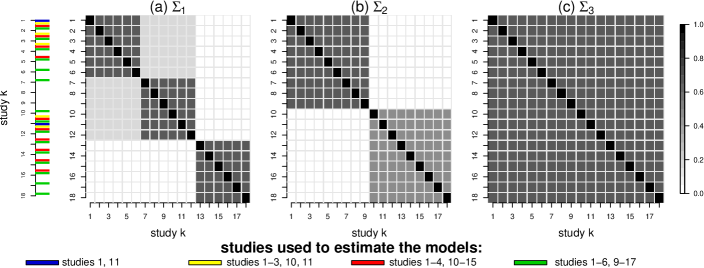
Figure 1: Similarity matrixes $\bm{\Sigma}=\bm{\Sigma}_{1},\bm{\Sigma}_{2},\bm{\Sigma}_{3}\in\mathbb{R}^{18\times 18}$ used to simulate the datasets. We simulated collections of $18$ datasets $\mathcal{D}=\{D_{k}\}_{k=1}^{18}$ with similarity matrix $\bm{\Sigma}$ for $\bm{\beta}.$ Studies indicated in blue (2 studies), yellow (5 studies), red (10 studies) or green (15 studies) are used to fit models with $K=2,5,10$ or $15$ studies.

Survival times where generated from proportional hazard models with baseline survival functions $\widehat{S}_{k}(\cdot)$, regression coefficients $\bm{\beta}_{k}$, and censoring survival functions $\widehat{S}_{C,k}(\cdot)$. Here $\widehat{S}_{k}(\cdot)$ and $\widehat{S}_{C,k}(\cdot)$ have been estimated from the ovarian cancer datasets that we discuss in Section 5. For each study $k$ we also generated an additional 1,000 observations, that were not used to fit regression models, but were used to evaluate predictions.

4.1 Estimation of $\Sigma$ and selection of $(\lambda_{1},\lambda_{0})$

We use initial estimates $\widehat{\bm{\beta}_{k}}$ obtained from $K$ independent ridge regression models to estimate $\bm{\Sigma}$. The procedure leverage the Bayesian interpretation (2) of the regularized likelihood (1). As formalized in (2), with $R_{1}\left(\bm{\beta}\right)=\sum_{j=1}^{p}||\bm{\beta}_{1:K,j}-\beta_{0,j}\bm{1}||^{a}_{\bm{\Sigma}},$ we can interpret $(\beta_{j,1},\cdots,\beta_{j,K}),j=1,\cdots,p$, as $p$ independent vectors each with covariance matrix $\bm{\Sigma}$. If the $\bm{\beta}_{k},k=1,\cdots,K,$ were known we could straightforwardly estimate $\bm{\Sigma}$. For instance with $a=2$, the parameters $(\beta_{j,1},\cdots,\beta_{j,K}),j=1,\cdots,p$ can be interpreted as independent multivariate normal vectors with mean zero and covariance matrix $\bm{\Sigma}$. The joint normal distribution implies that $E[\bm{\beta}_{k}|\{\bm{\beta}_{k^{\prime}}\}_{0<k^{\prime}\leq K,k^{\prime}\neq k}]=\sum_{0<k^{\prime}\leq K,k^{\prime}\neq k}\alpha_{k,k^{\prime}}\bm{\beta}_{k^{\prime}}$ where the weight vector $\bm{\alpha}_{k}=(\alpha_{k,k^{\prime}})_{0<k^{\prime}\leq K,k^{\prime}\neq k}$ is as function of $\bm{\Sigma}$ [18] for each $k=1,\cdots,K$. Therefore the conditional expectation of $\bm{X}_{k}\bm{\beta}_{k}$, given $\{\bm{\beta}_{k^{\prime}}\}_{0<k^{\prime}\leq K,k^{\prime}\neq k}$ is $\sum_{0<k^{\prime}\leq K,k^{\prime}\neq k}\alpha_{k,k^{\prime}}(\bm{X}_{k}\bm{\beta}_{k^{\prime}}).$ After replacing $\bm{\beta}_{k^{\prime}}$ with out initial estimates $\widehat{\bm{\beta}}_{k^{\prime}}$, we estimate $\bm{\alpha}_{k}$ via a Cox model with $K-1$ covariates $z_{k^{\prime}}=\bm{X}_{k}\widehat{\bm{\beta}}_{k^{\prime}}$ and regression coefficients $\bm{\alpha}_{k}$. We then use the empirical covariance matrix of $\bm{\beta}_{k}^{\star}=\sum_{0<k^{\prime}\leq K,k^{\prime}\neq k}\widehat{\alpha}_{k,k^{\prime}}\widehat{\bm{\beta}_{k}},k=1,\cdots,K$ as an estimate of $\bm{\Sigma}.$ Note that $\bm{\beta}_{k}^{\star}$ has a direct interpretation under the assumption that the independent vectors $(\beta_{1,j},\ldots,\beta_{K,j})$ are in a linear subspace with dimension less than $K$.

Figure 2 shows averages across the 100 simulations of the estimated similarity matrix between studies for the largest model with $K=15$ studies when $p_{0}=0$ (top row) and $p_{0}=0.9$ (bottom row). Figures 2 and 1 show that the algorithm of Section 4.1 on average recovers the similarity structure of the 15 studies.

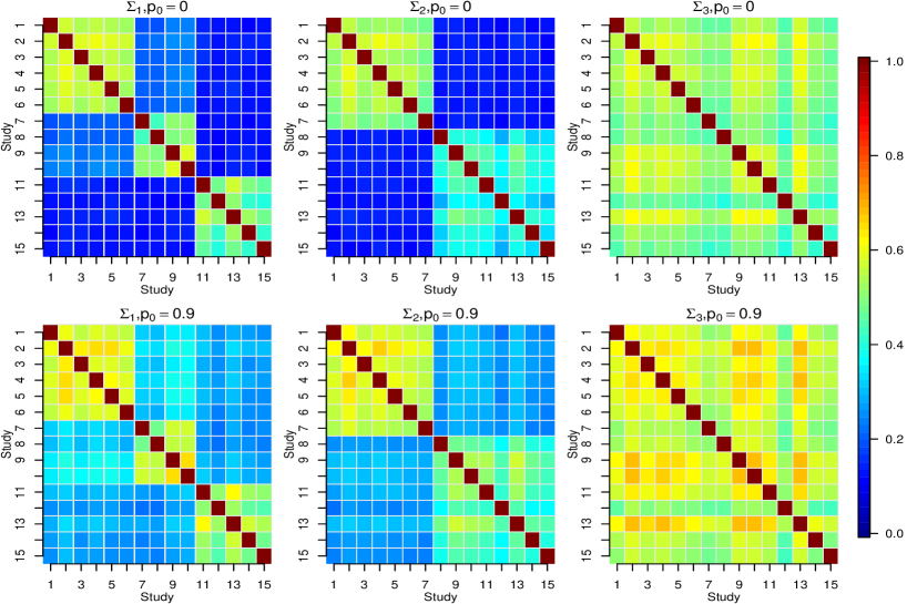
Figure 2: Average estimates across 100 simulations of the similarity matrix of the regression coefficients between the $K=15$ studies.

To select the parameters $\lambda_{0}$ and/or $\lambda_{1},$ we use Monte-Carlo cross-validation (CV) [42]. We evaluate candidate parameter estimates $\widehat{\bm{\beta}}$ using $\mathcal{C}(\widehat{\bm{\beta}})=\sum_{k}w_{k}\mathcal{C}(\widehat{\bm{\beta}}_{k},\mathcal{D}_{k}),$ where the C-statistics $\mathcal{C}(\widehat{\bm{\beta}}_{k},\mathcal{D}_{k})=\widehat{Pr}\Big{(}\bm{x}_{1}^{\prime}\widehat{\bm{\beta}}_{k}>\bm{x}^{\prime}_{2}\widehat{\bm{\beta}}_{k}|Y_{1}<Y_{2}\Big{)}$ is the estimated concordance [21, 36, 49] between two survival times $Y_{1}$ and $Y_{2}$ with covariate vectors $\bm{x}_{1}$ and $\bm{x}_{2}$ in population $k$. The weights $w_{k}\geq 0$ account for differences in study sample sizes, we used $w_{k}=1/\sqrt{m_{k}}$. We first split the data randomly $M$-times into training (80%) and validation (20%) datasets. Next we define a grid of tuning parameters $\bm{\lambda}=(\lambda_{1},\lambda_{0}).$ For each combination of tuning parameters $\bm{\lambda}$ of the grid, we estimate $\widehat{\bm{\beta}}^{(m)}$ based on the $m=1,\cdots,M$ CV training datasets (which are identical across different grid-points) and use the validation datasets to obtain estimates of the study-specific C-statistics $\mathcal{C}_{\lambda}(\widehat{\bm{\beta}}_{k}^{(m)},\mathcal{D}_{k}),m=1,\cdots,M$ for $\widehat{\bm{\beta}}_{k}^{(m)}$ with $\bm{\lambda}$. We then average these $M$ C-statistics and compute the overall estimate $\mathcal{C}_{\lambda}(\widehat{\bm{\beta}})$ for $\lambda$. Lastly, we select the $\lambda$-value with the highest average C-statistics $\mathcal{C}_{\lambda}(\widehat{\bm{\beta}}).$

4.2 Prediction Accuracy

Figure 3 shows, for each of the 18 studies box-plots of the estimated C-statistics [21, 36, 49] when either $2,5,10$ or $15$ studies (1st to 4th column) were used to estimate the similarity matrix and the model. C-statistics $\mathcal{C}(\widehat{\bm{\beta}}_{k},\mathcal{D}_{k})$ for studies $k$ that were utilized to estimate the model are highlighted inside the brown rectangles (estimated using the additional 1000 hold-out observations in study $k$), whereas C-statistics $\mathcal{C}(\widehat{\bm{\beta}}_{0},\mathcal{D}_{k})$ for studies $k$ that were not used to estimate the model are shown on the right of the brown rectangles.

The three rows of Figure 3 correspond to scenarios with data generated using $\bm{\Sigma}_{1}$ (top row of Figure 3), $\bm{\Sigma}_{2},$ (2nd row), or $\bm{\Sigma}_{3}$ (bottom row) as illustrated in Figure 1. Red, green and blue box-plots on the top-row indicate the three clusters of studies under $\bm{\Sigma}_{1}$. Similarly, red and green box-plots in the 2-nd row indicate the two clusters of studies under $\Sigma_{2}.$ Differences in the distribution of the C-statistics between studies within the same cluster are due to differences in the sample sizes $n_{k}$ and covariate matrixes $\bm{X}_{k}$, which remain identical across the simulated datasets.

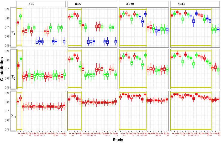
Figure 3: Predictions with the penalized regression model with $(a,\lambda_{0})=(2,0)$. We consider $\bm{\Sigma}=\bm{\Sigma}_{1},\bm{\Sigma}_{2}$ and $\bm{\Sigma}_{3}$ (see Figure 1), and $p_{0}=0$ across 100 simulations of a collection of 18 studies. Either $K=2,5,10$ or $15$ studies (studies inside the brown rectangles) were used for estimation/selection of $(\bm{\Sigma},\lambda_{1},\bm{\beta})$. The colors (red, green, blue) of the Box-plots indicate clusters of studies (3, 2, or 1 clusters when $\bm{\Sigma}=\bm{\Sigma}_{1}$, $\bm{\Sigma}_{2}$ or $\bm{\Sigma}_{3}$).

For $\bm{\Sigma}=\bm{\Sigma}_{1}$ (1st row of Figure 3), with three clusters of studies, predictions show improvements when the number of studies used to train the regression models increases $K$. For $K=2$ or $5$, all studies used for estimation belong to the first two clusters (red and green box-plots). In these two cases, for each study $k=13,\cdots 18$ in cluster 3 (blue box-plots) the inter-quartile range (IQR) of the C-statistics $\mathcal{C}(\widehat{\bm{\beta}}_{0},\mathcal{D}_{k})$ across simulations lies within the interval 0.52 to 0.55. Whereas for $K=10$ (3rd column, studies 1-4 and 10-15 are use for estimation), studies from all three clusters have been used for training. In this case, the IQRs of $\mathcal{C}(\widehat{\bm{\beta}}_{0},\mathcal{D}_{k})$ across simulations for all three hold-out studies $k=16,17,18$ in cluster 3 are within the interval 0.65 to 0.69. The last row of Figure 3 shows that, as expected, borrowing of information in the estimation of model parameters is most effective in the case of a single cluster of studies.

Next, we compared our estimates of $\bm{\beta}$ based on model (1), with $a=2$ for $R_{1}(\cdot)$ and ridge penalty (HR-R, $\lambda_{1}=0$) or LASSO penalty (HR-L, $\lambda_{2}=0$) for $\bm{\beta}_{0},$ to Cox models trained separately on each study $\mathcal{D}_{k}$ with LASSO (single-study LASSO, SL) or ridge penalties (single-study ridge, SR) for $\bm{\beta}_{k}$. In addition we consider two models that combine all (2, 5, 10 or 15) studies into a single dataset and estimate a single Cox model (with regression parameters $\bm{\beta}_{0}$) using a LASSO (pooled LASSO, PL) or ridge (pooled ridge, PR) penalty for the coefficients $\bm{\beta}_{0}.$ We also consider two meta-analysis approaches described in [51, 40] that combine study specific estimates $\widehat{\bm{\beta}}_{k}$ into a single vector $\widehat{\bm{\beta}}_{0}$ using either fixed effects (FE) or random-effects (RE) estimation.

Figures 4 and supplementary Figures A.1 and A.2 show the average C-statistics of each method when we used $K=5$ or $K=10$ studies for estimation. The pooled LASSO and ridge models (PL and PR) and the meta-analyses methods (FE and RE) estimate a single parameter $\bm{\beta}_{0}$, which was used to compute the C-statistics $C(\widehat{\bm{\beta}}_{0},\mathcal{D}_{k})$ for each study $k$. For the single-study SL and SR models we used the study-specific estimates $\widehat{\bm{\beta}}_{k}$ to compute $C(\widehat{\bm{\beta}}_{k},\mathcal{D}_{k})$ for in-study prediction (using the 1,000 validation observations). For prediction with SL and SR in studies $k^{\prime}$ not used for estimation, we used each estimate $\widehat{\bm{\beta}}_{k}$ of the $K=5$ (or 10) training studies for predictions $\mathcal{C}(\widehat{\bm{\beta}}^{k},\mathcal{D}_{k^{\prime}})$ in all hold-out studies $k^{\prime}$. For each hold-out studies $k^{\prime}$ we then averaged these $\mathcal{C}(\widehat{\bm{\beta}}^{k},\mathcal{D}_{k^{\prime}})$ over all $K=5$ (or 10) training studies, i.e. Figure 4 reportes $\sum_{k}\mathcal{C}(\widehat{\bm{\beta}}^{k},\mathcal{D}_{k^{\prime}})/K$ for studied $k^{\prime}$.

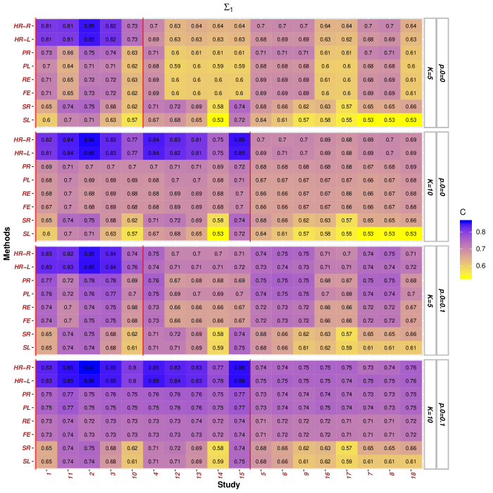
Figure 4: Average prediction across 100 simulations of a collection of 18 studies. Study specific effects $\bm{\beta}_{k}$ have been generated under $\bm{\Sigma}_{1}$ (see Figure 1). Either $5$ or $10$ of the 18 studies (studies in the left of the horizontal red bar) are used for the similarity matrix and covariate-effect estimation. See Figures A.1 and A.2 for results with similarity scenarios $\bm{\Sigma}_{2}$ and $\bm{\Sigma}_{3}$.

For studies $k$ used to train the model, both HR-L and HR-R improve predictions $C(\widehat{\bm{\beta}}_{k},\mathcal{D}_{k})$ substantially compared to single-study estimates SL and SR. For instance, with $K=5,p_{0}=0$ and unknown $\bm{\Sigma}=\bm{\Sigma}_{1}$ (three clusters of studies), the average difference between $C(\widehat{\bm{\beta}}_{k},\mathcal{D}_{k})$ of HR-R and SR is between 0.07 and 0.16 for each of the five studies (0.62 to 0.75 for SR compared to 0.73 to 0.85 for HR-R). Similarly, meta-analytic and pooled estimates FE, RE and PL, SL improve predictions on the $K=5$ datasets compared to single-study estimates, especially PR. But improvements are smaller than for HR-P and HR-L, with C-values on average (across simulations) between 0.08 to 0.15 below HR-R and HR-L models (for instance, 0.63 to 0.73 for PR compared to 0.73 to 0.85 for HR-R). When $K=10$ studies are used to estimate the models, results are similar to the setting with $K=5$ - meta-analytic, pooled and hierarchical estimates improve predictions over single-study estimates, with larger improvements for HR-R and HR-L estimates for in-study predictions.

In the case of a single cluster of studies ($\bm{\Sigma}=\bm{\Sigma}_{3}$, supplementary Figure A.2), with strong similarity of the study-specific parameters $\bm{\beta}_{k}$, pooling of studies to estimate a single $\bm{\beta}_{0}$ is expected to be the most favorable prediction approach. Therefore, PL, PR, HR-R and HR-L predict survival substantially better than the FE, RE, SL and SR methods (supplementary Figure A.2). With $p_{0}=0$, in-study predictions based on HR-R and HR-L estimates are on average slightly better than for PR and PL estimates (difference of 0.01 to 0.04 for HR-R compared to PR with $K=5$ studies, and 0.02 to 0.05 with $K=10$). Whereas PR, PL, HR-R and HR-L have similar average $C$-statistics for holdout studies.

5 Survival prediction in ovarian cancer

We applied model (1) to predict survival in ovarian cancer using the curatedOvarianData repository, a curated collection of gene-expression datasets [20]. To evaluate prediction, we split the largest study in the database, the TCGA dataset [32] with $510$ observations, 1,000 times randomly into a training dataset of $n_{1}=50,75,\ldots,$ or $300$ observations and a validation dataset with $510-n_{1}$ observations. We predicted patient survival $Y_{1,i}$ in the TCGA holdout data by leveraging the hierarchical regularization model (1) using five additional datasets $k=2,\cdots,K=6$ (PMID-17290060[17], GSE51088[26], MTAB386[2], GSE13876[15] and GSE19829 [27]) with sample sizes ranging between $n_{k}=42$ (GSE19829) and $157$ (GSE13876) observations. In all the analyses we used the expression values of the $p=3,030$ genes that are common in all six studies to predict patient survival.

To evaluate the hierarchical regularization method (1), we created different cross-study heterogeneity scenarios that are motivated by documented inconsistencies across cancer datasets and by possible pre-processing errors [33, 39, 4, 1, 38, 41]. This is achieved by introducing in one (scenario 2: GSE13876[15]) or two studies (scenario 3: GSE13876[15] and GSE19829 [27]) a distortion of the expression values $x_{k,i,j}$ which become $10-3x_{k,i,j},j=1,\ldots,p$ for study $k=K$ (scenario two) or studies $k=K-1,K$ (scenario three). In scenario one we used the covariates $x_{k,i,j}$ of the six studies.

Similar to Section 4, we consider parameter estimates based on the $n_{1}=50,\cdots,300$ TCGA training samples using (i) single study Cox models with LASSO (SL) or (ii) ridge (SR) regularization, pooled Cox regression models that combine the $n_{1}$ TCGA-observations and the remaining five studies (PMID-17290060, GSE51088, MTAB386, GSE13876 and GSE19829) into a single dataset with (iii) LASSO (PL) or (iv) ridge (PR) regularization, (v) fixed effects (FE) and (vi) random effects (RE) model meta-analyses models as described in [40, 3, 51], and (vii) the proposed hierarchical regularization model (1) with $\lambda_{0}=1,a=2$ (HR-R).

Single-study cox-models with LASSO-penalty trained on the TCGA data with $n_{1}=50$ data points had low average C-values of $0.505$ across the 1,000 generated training-validation samples, with minor improvements up $0.52$ when $n_{1}=300$ observations are used for model training. Single study ridge regression models performed substantially better, with average C-statistics ranging between $0.53$ for $n_{1}=50$ and $0.57$ for $n_{1}=300$ observations. Improvements in risk predictions through integration of additional studies vary substantially across data-integration methods and scenarios. For scenario 1, FE and RE meta-analyses have both nearly constant and identical average C-statistics of $0.57$ across all sample sizes $n_{1}$, while PL had an average C-statistics of $0.56$ for $n_{1}=50$ with minor improvements up to $0.57$ when $n_{1}=300.$ Both, HR-R and PR have similar prediction accuracy across sample sizes $n_{1},$ with identical average C-statistics of $0.60$ when $n_{1}=50$ and modest improvements up to $0.61$ for both, HR-R and PR, when $n_{1}=300$.

Figure 5 shows, for scenarios two and three, average C-statistics for the TCGA validation samples. Different curves correspond to different prediction methods. The black curves show the average C-statistics (y-axis) across the 1,000 TCGA validation samples of size $510-n_{1}$ for Cox models trained on $n_{1}=50,\cdots,300$ observations from the TCGA study (x-axis) using either SL (dotted curve) or SR (solid curve). The red curves show the average C-statistic for PR (solid curve) and PL (dotted curve) models, the green curves correspond to FE (dotted line) and RE (solid line) meta-analysis models, and the blue curve corresponds to the HR-R.

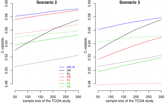
Figure 5: Average C-statistics for single-study SL and SR methods with $n_{1}=50,\cdots,300$ TCGA training samples, and for data-integration methods (PL, PR, FE, RE, HR-R) use the $n_{1}$ TCGA training samples and training samples from five additional studies (PMID-17290060, GSE51088, MTAB386, GSE13876 and GSE19829).

In scenario two, the RE meta-analysis, which combines estimates from the $n_{1}=50$ TCGA data points with estimates from the remaining five studies, has the same average C-statistics as the single-study SR model trained on $n_{1}=240$ patients. For sample sizes $n_{1}>250$, pooled regression models PR have similar performances as RE models. The HR-R model trained on $n_{1}=50$ TCGA patients has an average C-statistics the is superior to those of PR and FE procedures with $n_{1}=50,\cdots,300$. As expected, with increased discrepancies in the relations between covariates and outcomes across studies (scenario three), performances of all data-integration methods decrease. HR-R models with $n_{1}=50$ TCGA patients have similar average C-values as single study SR modes with $n_{1}\approx 200$ patients. PR, PL, FE and RE methods rely on the assumption that the regression parameters are similar across studies. With substantial departures from this assumption the hierarchical model HR-R shows, across all sample sizes $50\leq n_{1}\leq 300$, gains in average prediction accuracy compared to PR, PL, FE and RE.

6 Discussion

The analysis of relations between omics variables and time to event outcomes, and the use of individual profiles $\bm{x}_{k,i}$ for predictions, are particularly challenging when the sample size $n_{k}$ is small. These analyses often include thousands of potential predictors. The use of multiple studies and pooling of information can improve prediction accuracy. Meta-analyses can be utilized when the relations of covariates and outcomes are homogeneous across studies. But recent work in oncology [40, 51, 47] showed that there can be clusters of studies with relevant discrepancies in their covariate-outcome relations due, for example, to differences in study designs, patient populations and treatments.

We combined two established concepts, regularization of regression models [25, 45, 46, 19] and metrics of similarity between datasets [22] that identify clusters of studies. We used these concepts to estimate study-specific regression parameters $\bm{\beta}_{k}$ and for predictions, both in $k=1,\ldots,K$ contexts that are represented in our collection of datasets, for example $K$ distinct geographic regions, and in other contexts $(k=K+1)$ by estimating the latent parameters $\bm{\beta}_{0}$.

The $K\times K$ similarity matrix $\bm{\Sigma}$ is used to regularize the likelihood function, and it tunes the degree of borrowing of information in the estimation of $K$ study-specific regression models. It shrinks the estimate of the k-th study-specific regression parameter $\bm{\beta}_{k}$ towards estimates $\bm{\beta}_{k^{\prime}}$ of studies $k^{\prime}$ that are similar to study $k$ (large $\Sigma_{k,k^{\prime}}$). In contrast studies with low similarity ($\Sigma_{k,k^{\prime}}\approx 0$) have little influence on the estimation of $\bm{\beta}_{k}$. In our analyses we verified that, if there are clusters of studies with similar predictors-outcome relations, then the introduced method improves the accuracy of predictions compared to alternative procedures, including single-study estimates, meta-analyses and pooling of all studies into a single data matrix.

Funding

Lorenzo Trippa was partially supported by the NSF grant 1810829.

Appendix A Appendix

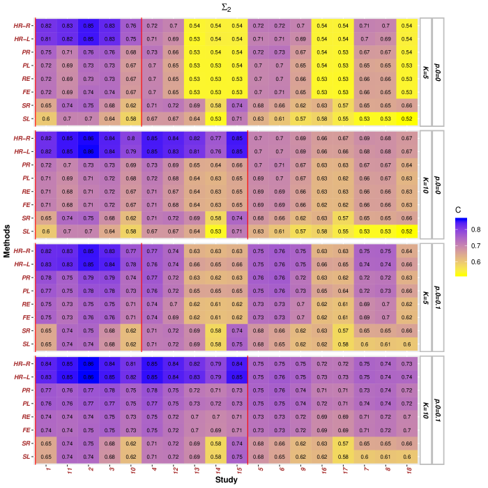
Figure A.1: Average prediction across 100 simulations of a collection of 18 studies. Study specific effects $\bm{\beta}_{k}$ have been generated under $\bm{\Sigma}_{2}.$ Either $5$ or $10$ of the 18 studies (studies in the left of the horizontal red bar) are used for the similarity matrix and covariate-effect estimation.

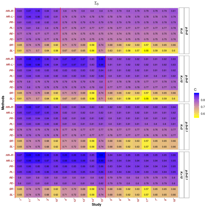
Figure A.2: Average prediction across 100 simulations of a collection of 18 studies. Study specific effects $\bm{\beta}_{k}$ have been generated under $\bm{\Sigma}_{3}.$ Either $5$ or $10$ of the 18 studies (studies in the left of the horizontal red bar) are used for the similarity matrix and covariate-effect estimation.

References

- Acharya et al. [2008] C. R. Acharya, D. S. Hsu, C. K. Anders, A. Anguiano, K. H. Salter, K. S. Walters, R. C. Redman, S. A. Tuchman, C. A. Moylan, S. Mukherjee, et al. Gene expression signatures, clinicopathological features, and individualized therapy in breast cancer. Jama, 299(13):1574–1587, 2008.
- Bentink et al. [2012] S. Bentink, B. Haibe-Kains, T. Risch, J.-B. Fan, M. S. Hirsch, K. Holton, R. Rubio, C. April, J. Chen, E. Wickham-Garcia, et al. Angiogenic mrna and microrna gene expression signature predicts a novel subtype of serous ovarian cancer. PloS one, 7(2), 2012.
- Bernau et al. [2014] C. Bernau, M. Riester, A.-L. Boulesteix, G. Parmigiani, C. Huttenhower, L. Waldron, and L. Trippa. Cross-study validation for the assessment of prediction algorithms. Bioinformatics, 30(12):i105–i112, 2014.
- Bonnefoi et al. [2007] H. Bonnefoi, A. Potti, M. Delorenzi, L. Mauriac, M. Campone, M. Tubiana-Hulin, T. Petit, P. Rouanet, J. Jassem, E. Blot, et al. Retracted: Validation of gene signatures that predict the response of breast cancer to neoadjuvant chemotherapy: a substudy of the eortc 10994/big 00-01 clinical trial, 2007.
- Bøvelstad et al. [2007] H. M. Bøvelstad, S. Nygård, H. L. Størvold, M. Aldrin, Ø. Borgan, A. Frigessi, and O. C. Lingjærde. Predicting survival from microarray data a comparative study. Bioinformatics, 23(16):2080–2087, 2007.
- Bøvelstad et al. [2009] H. M. Bøvelstad, S. Nygård, and Ø. Borgan. Survival prediction from clinico-genomic models-a comparative study. BMC bioinformatics, 10(1):1, 2009.
- Boyd et al. [2011] S. Boyd, N. Parikh, E. Chu, B. Peleato, and J. Eckstein. Distributed optimization and statistical learning via the alternating direction method of multipliers. Foundations and Trends® in Machine Learning, 3(1):1–122, 2011.
- Byrd et al. [1995] R. H. Byrd, P. Lu, J. Nocedal, and C. Zhu. A limited memory algorithm for bound constrained optimization. SIAM Journal on Scientific Computing, 16(5):1190–1208, 1995.
- Chen and Wang [2000] Y. Q. Chen and M.-C. Wang. Analysis of accelerated hazards models. Journal of the American Statistical Association, 95(450):608–618, 2000.
- Cheng et al. [2015] X. Cheng, W. Lu, and M. Liu. Identification of homogeneous and heterogeneous variables in pooled cohort studies. Biometrics, 71:397–403, 2015.
- Conlon et al. [2009] E. Conlon, B. Postier, B. Methe, K. Nevin, and D. Lovley. Hierarchical bayesian meta-analysis models for cross-platform microarray studies. Journal of Applied Statistics, 36(10):1067–1085, 2009.
- Conlon et al. [2006] E. M. Conlon, J. J. Song, and J. S. Liu. Bayesian models for pooling microarray studies with multiple sources of replications. BMC bioinformatics, 7(1):1, 2006.
- Conlon et al. [2012] E. M. Conlon, B. L. Postier, B. A. Methé, K. P. Nevin, and D. R. Lovley. A bayesian model for pooling gene expression studies that incorporates co-regulation information. PloS one, 7(12):e52137, 2012.
- Cox [1972] D. R. Cox. Regression models and life-tables. Journal of the Royal Statistical Society. Series B (Methodological), 34(2):187–220, 1972.
- Crijns et al. [2009] A. P. Crijns, R. S. Fehrmann, S. de Jong, F. Gerbens, G. J. Meersma, H. G. Klip, H. Hollema, R. M. Hofstra, G. J. te Meerman, E. G. de Vries, et al. Survival-related profile, pathways, and transcription factors in ovarian cancer. PLoS medicine, 6(2), 2009.
- DerSimonian and Laird [1986] R. DerSimonian and N. Laird. Meta-analysis in clinical trials. Controlled clinical trials, 7(3):177–188, 1986.
- Dressman et al. [2007] H. K. Dressman, A. Berchuck, G. Chan, J. Zhai, A. Bild, R. Sayer, J. Cragun, J. Clarke, R. S. Whitaker, L. Li, et al. An integrated genomic-based approach to individualized treatment of patients with advanced-stage ovarian cancer. Journal of Clinical Oncology, 25(5):517–525, 2007.
- Eaton [1983] M. L. Eaton. Multivariate statistics: a vector space approach. JOHN WILEY & SONS, 1983.
- Fu [1998] W. J. Fu. Penalized regressions: the bridge versus the lasso. Journal of computational and graphical statistics, 7(3):397–416, 1998.
- Ganzfried et al. [2013] B. F. Ganzfried, M. Riester, B. Haibe-Kains, T. Risch, S. Tyekucheva, I. Jazic, X. V. Wang, M. Ahmadifar, M. J. Birrer, G. Parmigiani, et al. curatedovariandata: clinically annotated data for the ovarian cancer transcriptome. Database, 2013, 2013.
- Harrell Jr et al. [1984] F. E. Harrell Jr, K. L. Lee, R. M. Califf, D. B. Pryor, and R. A. Rosati. Regression modelling strategies for improved prognostic prediction. Statistics in medicine, 3(2):143–152, 1984.
- Hastie et al. [2009] T. Hastie, R. Tibshirani, and J. Friedman. The Elements of Statistical Learning: Data Mining, Inference, and Prediction. Springer, 2009.
- Hastie et al. [2015] T. Hastie, R. Tibshirani, and M. Wainwright. Statistical learning with sparsity: the lasso and generalizations. Chapman and Hall/CRC, 2015.
- Hedges and Olkin [2014] L. V. Hedges and I. Olkin. Statistical methods for meta-analysis. Academic press, 2014.
- Hoerl and Kennard [1970] A. E. Hoerl and R. W. Kennard. Ridge regression: Biased estimation for nonorthogonal problems. Technometrics, 12(1):55–67, 1970.
- Karlan et al. [2014] B. Y. Karlan, J. Dering, C. Walsh, S. Orsulic, J. Lester, L. A. Anderson, C. L. Ginther, M. Fejzo, and D. Slamon. Postn/tgfbi-associated stromal signature predicts poor prognosis in serous epithelial ovarian cancer. Gynecologic oncology, 132(2):334–342, 2014.
- Konstantinopoulos et al. [2010] P. A. Konstantinopoulos, D. Spentzos, B. Y. Karlan, T. Taniguchi, E. Fountzilas, N. Francoeur, D. A. Levine, and S. A. Cannistra. Gene expression profile of brcaness that correlates with responsiveness to chemotherapy and with outcome in patients with epithelial ovarian cancer. Journal of clinical oncology, 28(22):3555, 2010.
- Liu et al. [2011] F. Liu, D. Dunson, and F. Zou. High-dimensional variable selection in meta-analysis for censored data. Biometrics, 67(2):504–512, 2011.
- Liu et al. [2013] M. Liu, W. Lu, V. Krogh, G. Hallmans, T. V. Clendenen, and A. Zeleniuch-Jacquotte. Estimation and selection of complex covariate effects in pooled nested case–control studies with heterogeneity. Biostatistics, 14(4):682–694, 2013.
- Ma et al. [2011a] S. Ma, J. Huang, and X. Song. Integrative analysis and variable selection with multiple high-dimensional data sets. Biostatistics, 12(4):763–775, 2011a.
- Ma et al. [2011b] S. Ma, J. Huang, F. Wei, Y. Xie, and K. Fang. Integrative analysis of multiple cancer prognosis studies with gene expression measurements. Statistics in medicine, 30(28):3361–3371, 2011b.
- Network et al. [2011] C. G. A. R. Network et al. Integrated genomic analyses of ovarian carcinoma. Nature, 474(7353):609, 2011.
- of Health and Services [2015] N. D. of Health and H. Services. Findings of research misconduct. NIH Guide Grants Contracts, 16(021), 2015.
- Park and Hastie [2007] M. Y. Park and T. Hastie. L1-regularization path algorithm for generalized linear models. Journal of the Royal Statistical Society: Series B (Statistical Methodology), 69(4):659–677, 2007.
- Park and Casella [2008] T. Park and G. Casella. The bayesian lasso. Journal of the American Statistical Association, 103(482):681–686, 2008.
- Pencina and D’Agostino [2004] M. J. Pencina and R. B. D’Agostino. Overall c as a measure of discrimination in survival analysis: model specific population value and confidence interval estimation. Statistics in medicine, 23(13):2109–2123, 2004.
- Polson et al. [2015] N. G. Polson, J. G. Scott, B. T. Willard, et al. Proximal algorithms in statistics and machine learning. Statistical Science, 30(4):559–581, 2015.
- Potti et al. [2006a] A. Potti, A. Bild, H. K. Dressman, D. A. Lewis, J. R. Nevins, and T. L. Ortel. Gene-expression patterns predict phenotypes of immune-mediated thrombosis. Blood, 107(4):1391–1396, 2006a.
- Potti et al. [2006b] A. Potti, H. K. Dressman, A. Bild, R. F. Riedel, G. Chan, R. Sayer, J. Cragun, H. Cottrill, M. J. Kelley, R. Petersen, et al. Genomic signatures to guide the use of chemotherapeutics. Nature medicine, 12(11):1294–1300, 2006b.
- Riester et al. [2014] M. Riester, W. Wei, L. Waldron, A. C. Culhane, L. Trippa, E. Oliva, S.-h. Kim, F. Michor, C. Huttenhower, G. Parmigiani, et al. Risk prediction for late-stage ovarian cancer by meta-analysis of 1525 patient samples. Journal of the National Cancer Institute, page dju048, 2014.
- Salter et al. [2008] K. H. Salter, C. R. Acharya, K. S. Walters, R. Redman, A. Anguiano, K. S. Garman, C. K. Anders, S. Mukherjee, H. K. Dressman, W. T. Barry, et al. An integrated approach to the prediction of chemotherapeutic response in patients with breast cancer. PLoS One, 3(4):e1908–e1908, 2008.
- Shao [1993] J. Shao. Linear model selection by cross-validation. Journal of the American statistical Association, 88(422):486–494, 1993.
- Simon et al. [2011] N. Simon, J. Friedman, T. Hastie, and R. Tibshirani. Regularization paths for cox’s proportional hazards model via coordinate descent. Journal of statistical software, 39(5):1, 2011.
- Sinha et al. [2003] D. Sinha, J. G. Ibrahim, and M. Chen. A bayesian justification of cox’s partial likelihood. Biometrika, 90(3):629–641, 2003. doi: 10.1093/biomet/90.3.629. URL +http://dx.doi.org/10.1093/biomet/90.3.629.
- Tibshirani [1996] R. Tibshirani. Regression shrinkage and selection via the lasso. Journal of the Royal Statistical Society. Series B (Methodological), pages 267–288, 1996.
- Tibshirani [1997] R. Tibshirani. The lasso method for variable selection in the cox model. Statistics in Medicine, 16(4):385–395, 1997.
- Trippa et al. [2015a] L. Trippa, L. Waldron, C. Huttenhower, and G. Parmigiani. Bayesian nonparametric cross-study validation of prediction methods. Ann. Appl. Stat., 9(1):402–428, 03 2015a. doi: 10.1214/14-AOAS798.
- Trippa et al. [2015b] L. Trippa, L. Waldron, C. Huttenhower, G. Parmigiani, et al. Bayesian nonparametric cross-study validation of prediction methods. The Annals of Applied Statistics, 9(1):402–428, 2015b.
- Uno et al. [2011] H. Uno, T. Cai, M. J. Pencina, R. B. D’Agostino, and L. Wei. On the c-statistics for evaluating overall adequacy of risk prediction procedures with censored survival data. Statistics in medicine, 30(10):1105–1117, 2011.
- Van Wieringen et al. [2009] W. N. Van Wieringen, D. Kun, R. Hampel, and A.-L. Boulesteix. Survival prediction using gene expression data: a review and comparison. Computational statistics & data analysis, 53(5):1590–1603, 2009.
- Waldron et al. [2014] L. Waldron, B. Haibe-Kains, A. C. Culhane, M. Riester, J. Ding, X. V. Wang, M. Ahmadifar, S. Tyekucheva, C. Bernau, T. Risch, et al. Comparative meta-analysis of prognostic gene signatures for late-stage ovarian cancer. Journal of the National Cancer Institute, 106(5):dju049, 2014.
- Wang and Leng [2008] H. Wang and C. Leng. A note on adaptive group lasso. Computational Statistics & Data Analysis, 52(12):5277 – 5286, 2008. ISSN 0167-9473. doi: http://dx.doi.org/10.1016/j.csda.2008.05.006. URL http://www.sciencedirect.com/science/article/pii/S0167947308002582.
- Wei [1992] L. Wei. The accelerated failure time model: a useful alternative to the cox regression model in survival analysis. Statistics in medicine, 11(14-15):1871–1879, 1992.
- Zou and Hastie [2005] H. Zou and T. Hastie. Regularization and variable selection via the elastic net. Journal of the royal statistical society: series B (statistical methodology), 67(2):301–320, 2005.