Critical behavior of the classical spin-1 Ising model: a combined low-temperature series expansion and Metropolis Monte Carlo analysis

Abstract

In this paper, we theoretically study the critical properties of the classical spin-1 Ising model using two approaches: 1) the analytical low-temperature series expansion and 2) the numerical Metropolis Monte Carlo technique. Within this analysis, we discuss the critical behavior of one-, two- and three-dimensional systems modeled by the first-neighbor spin-1 Ising model for different types of exchange interactions. The comparison of the results obtained according the Metropolis Monte Carlo simulations allows us to highlight the limits of the widely used mean-field theory approach. We also show, via a simple transformation, that for the special case where the bilinear and bicubic terms are set equal to zero in the Hamiltonian the partition function of the spin-1 Ising model can be reduced to that of the spin-1/2 Ising model with temperature dependent external field and temperature independent exchange interaction times an exponential factor depending on the other terms of the Hamiltonian and confirm this result numerically by using the Metropolis Monte Carlo simulation. Finally, we investigate the dependence of the critical temperature on the strength of long-range interactions included in the Ising Hamiltonian comparing it with that of the first-neighbor spin-1/2 Ising model.

I Introduction

The classical spin-1/2 Ising model with nearest neighbor interactions for a lattice with $N$ sites was suggested by Lenz in 1920’s is defined by the following Hamiltonian Ising (1925)

$${\mathcal{H}_{\rm{spin}1/2}}=-J\sum_{<ij>}s_{i}s_{j}-H\sum_{i=1}^{N}s_{i},$$ (1)

where $s_{i}=+1$ or $-1$ is the spin variable. The notation $<ij>$ indicates a sum over nearest neighbors lattice sites, $J$ is the exchange constant which gives the interaction strength between two neighboring spins and $H$ is an external field applied to each degree of freedom. Ising solved the one-dimensional (1D) model in 1924 and, on the basis of the fact that 1D system had no phase transition, he wrongly asserted that there was no phase transition in any dimension Ising (1925); Brush (1967). Peierls proved that the model exhibits a phase transition in two or higher-dimensional lattices Peierls and Born (1936). The exact solution was found by Onsager Onsager (1944); Baxter (2012)and Yang Yang (1952) using algebraic approach and transfer matrix method. According to this analytical solution, in the two-dimensional (2D) square lattice a second-order phase transition at some critical temperature $T_{c}$ takes place when an external field $H$ tends to zero. This is in agreement with the result of the series expansion method Yeomans (1993) and Monte Carlo simulations Newman (1999). Although there’s no exact solution for three-dimensional (3D) lattices, it is possible to find the critical temperature and critical exponents of the model using numerical methods like Monte Carlo simulations Newman (1999); Sonsin et al. (2015).

Spin-1/2 Ising model is appropriate to describe systems in which each degree of freedom has two states, but for systems with three states the spin-1 Ising model is more suitable Yeomans (1993). In the last decades, efforts have been made to study theoretically the underlying physics predicted by the spin-1 Ising model using mean-field theories and effective field theories Kaneyoshi and Mielnicki (1990). In particular, the mean-field solution in the presence of a random crystal field and the effects of the magnitude of the crystal field on the critical properties have been investigated. Benyoussef et al. (1987); Kaneyoshi (1987, 1988); Boccara et al. (1989)

On the other hand, the behavior of the tricritical point as a function of crystal-field interactions for honeycomb and its dependence on the strength of biquadratic and bilinear exchange interactions in square and cubic lattices have been studied by using the effective-field theory Kaneyoshi (1986); Tucker (1989). Recently, an analysis of spin-1 Ising model including only the bilinear term on tetrahedron recursive lattices with arbitrary values of the coordination number has been performed to find an equation for the exact determination of the critical points and all critical phases Jurčišinová and Jurčišin (2016). ${\rm{He}^{3}-\rm{He}^{4}}$ mixture can be considered as spin-1 Ising model and some features of the mixture such as the $\lambda$ transition and the phase diagram of the mixture are described by the model Blume et al. (1971). However, despite their relevant results the above mentioned works focus on specific aspects of the critical properties of the spin-1 Ising model.

In this paper a systematic investigation of the critical properties exhibited by 1D, 2D (square) and 3D (cubic) systems modeled via the spin-1 classical Ising model Hamiltonian for different exchange interactions is performed overcoming some of the restrictions of the previous studies. The analytical investigation is carried out by using the low-temperature series expansion method applied to to the partition function. This is achieved after determining the counts and the Boltzmann weights of the partition function depending on the full Hamiltonian of the classical spin-1 Ising model on both a square (2D) and on a cubic lattice (3D).

The results obtained using the low-temperature series expansion method are compared to the numerical ones determined via Metropolis Monte Carlo simulations. The comparison of the exact Monte Carlo results with the ones derived using the approximated mean-field theory allows to highlight the limits of the latter approach that was widely used in the past decades as mentioned above.

The most general form of Hamiltonian of the spin-1 Ising model for a lattice with $N$ spin is Yeomans (1993)

$${\mathcal{H}_{\rm{spin1}}}=-J\sum_{<ij>}s_{i}s_{j}-K\sum_{<ij>}s_{i}^{2}s_{j}^{2}-D\sum_{i=1}^{N}s_{i}^{2}$$

$$-L\sum_{<ij>}(s_{i}^{2}s_{j}+s_{i}s_{j}^{2})-H\sum_{i=1}^{N}s_{i},$$ (2)

where $s_{i}=+1$ or $0$ or $-1$, $K$ is the biquadratic coefficient, $D$ is the anisotropy coefficient and $L$ is the bi-cubic coefficient. Note that all coefficient appearing in (I) have the dimension of an energy. Sums are extended to the $N$ degrees of freedom and if the coefficients in (I) are chosen to be positive, the ground state energy of the system corresponds to the configuration in which for all $i^{\prime}s$ we have $s_{i}=+1$. As the spin-1/2 model the 1D classical spin-1 Ising model does not exhibit any phase transition at finite temperatures. In order to prove this claim we consider a 1D chain of spins with periodic boundary conditions. The free energy of the system, $F$ with entropy $S$ and energy $E$ at temperature $T$ by definition is given by Huang and Beale (1988):

$$F=E-TS=E-k_{B}T\ln\Omega,$$ (3)

where $k_{B}$ is Boltzmann constant and $\Omega$ is the number of configurations with energy $E$. Since we assume that all coefficients in (I) are non-negative, in the ground state all spin variables are up, i.e. for each site denoted by index $i$ we have $s_{i}=+1$ and the ground state configuration is $C=(+++...+++)$ where + means spin up. Hence, the energy and free energy of this configuration defined by $E_{0}$ and $F_{0}$ are

$$F_{0}=E_{0}=-N(H+D+J+K+2L).$$ (4)

Now, by flipping one of the spins to $0$ or $-1$, the system will assume another configuration, which must have higher free energy with respect to ground state configuration $C$ in order to undertake a phase transition at $T\neq 0$. We denote these two possible configurations by $C_{1}=(++...++-++...++)$ and $C_{1}^{{}^{\prime}}=(++...++\ 0++...++)$ where $-$ and $0$ mean spin down and spin-less respectively. The free energies, $F_{1}$ and $F_{1}^{{}^{\prime}}$, associated with these configurations are

$$F_{1}=E_{0}+4J+4L+2H-k_{B}T\ln N,$$ (5)

$$F_{1}^{{}^{\prime}}=E_{0}+2J+4L+H-k_{B}T\ln N.$$ (6)

In both cases, in the thermodynamic limit and for $T\neq 0$ we get $F_{1},F_{1}^{{}^{\prime}}<F_{0}$. Thus, the 1D version of spin-1 Ising model does not exhibit any phase transition at non-zero temperatures. However, for higher dimensions the system described by the spin-1 Ising model exhibits a phase transition and, due to its enlarged parameter space, a much richer variety of critical behavior with respect to the spin-1/2 counterpart Yeomans (1993). Since the study of the 2D and 3D spin-1 Ising model in its general form using either numerical or analytical tools becomes very interesting but at the same time very complicated, its critical behavior has only been studied in a few special cases in the literature. In one case just $J$ and $H$ are assumed different from zero and the system described by this spin-1 Ising model has been solved by applying low-temperature series expansion Enting et al. (1994); Fox and Guttmann (1973). In another case the spin-1 Ising model with non-vanishing $J$, $D$, and $K$ has been investigated by using mean-field approximation Blume et al. (1971). The latter one has been studied for $K=0$ by other methods like series expansion Saul et al. (1974), renormalization group theory Yeomans and E. Fisher (1981), and Monte Carlo simulation K. Jain (1980); Care (1993).

The paper is organized as follows. In section $2$ we shortly introduce the analytical and numerical methods applied to the spin-1 Ising model. In Section $3$ we firstly study the critical behavior of the classical spin-1 Ising model with nearest neighbor interaction in 2D square and 3D cubic lattices, respectively comparing some critical features with those of the spin-1/2 Ising model, then last part of section $3$ deals with the long-range spin-1 Ising model and the dependence of the critical temperature on the strength of long-range interactions. Finally, section $4$ is devoted to the conclusions.

II Methods

In this section we briefly discuss the analytical and numerical approaches we have used to analyze the classical spin-1 Ising model. In the first and second subsections we describe the mean-field theory and the low-temperature series expansion methods as representative analytical methods. The third subsection is a short description of the Metropolis Monte Carlo simulation which is a strong numerical tool that enables us to investigate the critical properties of the system.

II.1 Mean-field theory

We use a systematic way of deriving the mean-field theory for some Hamiltonian $\mathcal{H}$ in arbitrary dimension and coordinate number $z$ (cf. Yeomans (1993) where Mean-field theories are studied). We begin from the Bogoliubov inequality

$$F\leq\Phi=F_{0}+<\mathcal{H}-\mathcal{H}_{0}>_{0},$$ (7)

where $F$ is the true free energy of the system, $\mathcal{H}_{0}$ is a trial Hamiltonian depending on some variational parameters which we will introduce, $F_{0}$ is the corresponding free energy, and $<...>_{0}$ denotes an average taken in the ensemble defined by $\mathcal{H}_{0}$. The mean-field free energy, $F_{\rm{MF}}$, is then defined by minimizing $\Phi$ with respect to the variational parameters. In order to see how this method works let us consider the most general form of the classical spin-1 Ising model given by (I). We introduce the trial Hamiltonian as the following

$$\mathcal{H}_{0}=-H_{0}\sum_{i=1}^{N}s_{i}-D_{0}\sum_{i=1}^{N}s_{i}^{2}.$$ (8)

Hence, there are two variational parameters, $H_{0}$ and $D_{0}$, which will be determined by minimizing the functional $\Phi$. Assuming that the lattice is translationally invariant it is straightforward to find the partition function and the mean-field free energy. Consequently one can easily compute the magnetization, $M=<s_{i}>_{0}$ defined in dimensionless units as the thermal average of the spin variable and the thermal average of the square of the spin variable $\tau=<s_{i}^{2}>_{0}$ as follows

$$M=\frac{2e^{\beta(D+LzM+Kz\tau)}\sinh[\beta(JzM+H+Lz\tau)]}{1+2e^{\beta(D+LzM+Kz\tau)}\cosh[\beta(JzM+H+Lz\tau)]},$$

$$\tau=\frac{2e^{\beta(D+LzM+Kz\tau)}\cosh[\beta(JzM+H+Lz\tau)]}{1+2e^{\beta(D+LzM+Kz\tau)}\cosh[\beta(JzM+H+Lz\tau)]}.$$

Solving two self consistent equations (II.1) and (II.1) simultaneously, one can find the mean-field magnetization as a function of the temperature.

We remind that, although the use of mean-field theory gives us some valuable information about the behavior of the system and specifically it allows us to reproduce the phase diagram of the model in a relatively simple and qualitative way, from a quantitative point of view the results are not generally exact for the case of 2D and 3D lattices so that in this case we need to use more precise analytical and numerical methods allowing us to have a more exact knowledge of the critical behavior of these systems also quantitatively.

II.2 low-temperature series expansion method

Another possible way to investigate the spin-1 Ising model is to use low-temperature series expansion. The idea is to start from a completely ordered configuration, i.e. the ground state, and then flip spins one by one, and take all the configurations into account to compute the partition function, $Z$ as the following: Huang and Beale (1988)

$$Z=e^{-\frac{E_{0}}{k_{B}T}}(1+\sum_{n=1}^{\infty}\Delta Z_{N}^{(n)}),$$ (11)

where $E_{0}$ is ground state energy, and $\Delta Z_{N}^{(n)}$ is the sum of Boltzmann factors with energy that is measured with respect to the ground state energy when $n$ spins are flipped starting from the ground state configuration. Two factors contribute to the Boltzmann factor $\Delta Z_{N}^{(n)}$, namely the number of ways of flipping $n$ spins with a specific Boltzmann weight, or counts, and the corresponding Boltzmann weights Huang and Beale (1988).

Table 1: The counts and the Boltzmann weights contributing to the to the low-temperature series expansion of the partition function of a square lattice classical spin-1 Ising model for different numbners of flipped spins ($N_{f}$).

$N_{f}$	Count	Boltzmann weight
$1$	$N$	$x^{8}y^{2}z^{8}$
$1$	$N$	$x^{4}yz^{8}uw^{4}$
$2$	$2N$	$x^{12}y^{4}z^{16}$
$2$	$4N$	$x^{10}y^{3}z^{14}uw^{4}$
$2$	$2N$	$x^{7}y^{2}z^{14}u^{2}w^{7}$
$2$	$N(N-5)/2$	$x^{16}y^{4}z^{16}$
$2$	$N(N-5)$	$x^{12}y^{3}z^{16}uw^{4}$
$2$	$N(N-5)/2$	$x^{8}y^{2}z^{16}u^{2}w^{8}$
$3$	$2N$	$x^{16}y^{6}z^{24}$
$3$	$4N$	$x^{14}y^{5}z^{22}uw^{4}$
$3$	$2N$	$x^{16}y^{5}z^{20}uw^{4}$
$3$	$4N$	$x^{13}y^{4}z^{20}u^{2}w^{7}$
$3$	$2N$	$x^{12}y^{4}z^{20}u^{2}w^{8}$
$3$	$2N$	$x^{10}y^{3}z^{20}u^{3}w^{10}$
$3$	$4N$	$x^{16}y^{6}z^{24}$
$3$	$8N$	$x^{14}y^{5}z^{22}uw^{4}$
$3$	$4N$	$x^{16}y^{5}z^{20}uw^{4}$
$3$	$8N$	$x^{13}y^{4}z^{20}u^{2}w^{7}$
$3$	$4N$	$x^{12}y^{4}z^{20}u^{2}w^{8}$
$3$	$4N$	$x^{10}y^{3}z^{20}u^{3}w^{10}$
$3$	$2N(N-8)$	$x^{20}y^{6}z^{24}$
$3$	$2N(N-8)$	$x^{16}y^{5}z^{24}uw^{4}$
$3$	$4N(N-8)$	$x^{18}y^{5}z^{22}uw^{4}$
$3$	$2N(N-8)$	$x^{15}y^{4}z^{22}u^{2}w^{7}$
$3$	$4N(N-8)$	$x^{14}y^{4}z^{22}u^{2}w^{8}$
$3$	$2N(N-8)$	$x^{11}y^{3}z^{22}u^{3}w^{11}$
$3$	$N(N^{2}-15N+62)/6$	$x^{24}y^{6}z^{24}$
$3$	$N(N^{2}-15N+62)/2$	$x^{20}y^{5}z^{24}uw^{4}$
$3$	$N(N^{2}-15N+62)/2$	$x^{16}y^{4}z^{24}u^{2}w^{8}$
$3$	$N(N^{2}-15N+62)/6$	$x^{12}y^{3}z^{24}u^{3}w^{12}$
$4$	$N$	$x^{12}y^{4}z^{24}u^{4}w^{12}$
$4$	$18N$	$x^{13}y^{4}z^{26}u^{4}w^{13}$

We consider the spin-1 Ising model described by the Hamiltonian (I) for a square lattice as an example. For the sake of simplicity, we introduce the following parameters

$$x=e^{-\beta J},y=e^{-\beta H},z=e^{-\beta L},u=e^{-\beta D},w=e^{-\beta K},$$

where $\beta=\frac{1}{k_{B}T}$. Then we need to calculate the counts for different configurations. The computation of the counts is more complicated with respect to that of the spin-1/2 Ising model because in the spin-1 Ising model each spin can choose among three possible states. Table 1 shows Boltzmann weights and their counts for some configurations in which a few spins are flipped. Starting from these calculations summarized in Table 1 we finally obtain the low-temperature series expansion of the partition function for the spin-1 Ising model :

$$Z_{\rm{spin1}}^{\rm{square}}= e^{-\beta E_{0}}\bigg{(}1+Nx^{4}yz^{8}uw^{4}+2Nx^{7}y^{2}z^{14}u^{2}w^{7}+$$

$$Nx^{8}y^{2}z^{8}-\frac{5N}{2}x^{8}y^{2}z^{16}u^{2}w^{8}+4Nx^{10}y^{3}z^{14}uw^{4}+$$

$$6Nx^{10}y^{3}z^{20}u^{3}w^{10}-16Nx^{11}y^{3}z^{22}u^{3}w^{11}+$$

$$2Nx^{12}y^{4}z^{16}-5Nx^{12}y^{3}z^{16}uw^{4}+$$

$$6Nx^{12}y^{4}z^{20}u^{2}w^{8}+\frac{31N}{3}x^{12}y^{3}z^{24}u^{3}w^{12}+$$

$$Nx^{12}y^{4}z^{24}u^{4}w^{12}+12Nx^{13}y^{4}z^{20}u^{2}w^{7}+$$

$$18Nx^{13}y^{4}z^{26}u^{4}w^{13}+O(x^{14})\bigg{)}$$ (13)

We will follow the same procedure by finding the Boltzmann weights and the associated counts for the 3D cubic lattice in one of the special cases outlined in section $3$.

II.3 Metropolis Monte Carlo method

Monte Carlo method is a powerful numerical tool widely used to evaluate discrete spin models like Ising models to investigate the behavior of the associated thermodynamic functions of the models. It is also very popular to study continuous spin systems like XY and Heisenberg model, fluids, polymers, disordered materials, and lattice gauge theories (cf. Binder and Heermann (1997) where Monte Carlo Methods are studied). In this paper we use Metropolis Monte Carlo simulation. The algorithm can be summarized in three steps:

1. Set up of the lattice sites. To do it, for example in the case of 2D square lattice, we define a 2D array with $l_{x}\times l_{x}$ spin, which is called spin$[i][j]$, where $i$ and $j$ determine a specific lattice site.

2. Initialization of the system. We use a function named init $(l_{x}$, $J$, $K$, $D$, $L$, $H)$ to set the initial state of the system, which in principal can be chosen arbitrarily. In the simulations we choose a completely ordered state as the initial state with maximum magnetization. In this function, $l_{x}$ is the number of spins in each direction, and $J$, $K$, $D$, $L$, and $H$ are the values of the coefficients in the Hamiltonian of the spin-1 Ising model given by equation (I).

3. Use of a main loop in the main program to update the system many times. The function mc$(T)$ takes the temperature $T$ and uses Metropolis update. This function at first chooses randomly one of the spins in the lattice and flips that spin. For instance, if the randomly chosen spin is $+1$ it is flipped to $0$ or $-1$ with the same probability. The probability that the system is allowed to move from the initial state to the final state is

$$P(\mathrm{initial}\to\mathrm{final})=\begin{cases}1,\ \ \text{if}\ \ E_{\mathrm{final}}<E_{\mathrm{initial}}\\ e^{({-\beta(E_{\mathrm{final}}-E_{\mathrm{initial}}}))},\ \ \ \text{otherwise}\\ \end{cases}$$

By updating the system a sufficient number of times, it eventually reaches the equilibrium state at any temperature. Finally, it is possible to determine the thermodynamic functions such as magnetization, and susceptibility using following formulas Newman (1999):

$$M=\frac{1}{N}\sum_{i=1}^{N}s_{i},$$ (14)

$$\chi=\frac{1}{k_{B}T}(<M^{2}>-<M>^{2}).$$ (15)

III Results and discussions: special cases of spin-1 Ising Hamiltonian for 2D square and 3D cubic lattices

Owing to the previous arguments, in principle we know how to calculate the partition function associated with (I) expressing the Hamiltonian of the spin-1 Ising model and consequently we can characterize thermodynamically the model. However, since the general form of the Hamiltonian is very complex and the number of parameters appearing in the parameter space is high, it is not possible to study analytically and/or numerically in an exact way the critical behavior of the full Hamiltonian. It is thus useful to understand better the critical behavior of the spin-1 Ising model focusing our attention on some special cases with a lower number of parameters that are numerically solvable. These cases will be discussed in the following subsections. In the last subsection we will introduce the long-range spin-1 Ising model in analogy with the well-known spin-1/2 model to find out how its critical temperature depends on the magnitude of the long-range interaction.

III.1 Case 1

In this subsection, we restrict ourselves to the specific case in which all the coefficients in (I) are zero except $J$ and $H$, so that the Hamiltonian is given by

$${\mathcal{H}_{\rm{Ising1}}^{(1)}}=-J\sum_{<ij>}s_{i}s_{j}-H\sum_{i=1}^{N}s_{i}.$$ (16)

In this special case, the series expansion of the partition function for a 2D square lattice is obtained by setting $D$, $K$, and $L$ zero in (13). Let’s write down the free energy $F$, the magnetization $M$, and the susceptibility $\chi$ as follows Huang and Beale (1988)

$$F=-k_{B}T\ln Z,$$ (17)

$$M=-\frac{1}{N}\lim_{H\to 0}\left(\frac{\partial F}{\partial H}\right)_{T},$$ (18)

$$\chi=\frac{1}{N\beta}\lim_{H\to 0}\left(\frac{\partial^{2}\ln Z}{\partial H^{2}}\right)_{T}.$$ (19)

Now we can write down the series expansion of $M$, and $\chi$ for the square lattice:

$$M_{\rm{square}}^{(1)}= 1-x^{4}-4x^{7}+3x^{8}-30x^{10}+48x^{11}-52x^{12}$$

$$-120x^{13}+O(x^{14}),$$ (20)

$$\chi_{\rm{square}}^{(1)}= \beta(x^{4}+8x^{7}-6x^{8}+90x^{10}-144x^{11}+192x^{12}$$

$$+480x^{13}+O(x^{14})).$$ (21)

Likewise, one can find corresponding expressions for a 3D lattice. For simplicity we take a simple cubic lattice with each site having $z=6$ nearest neighbors. Since the procedure is similar to what we have done for square lattice we only write down the final expression of the above quantities as follows:

$$Z^{(1)}_{\rm{cube}} =e^{-\frac{E_{0}}{k_{B}T}}\bigg{[}1+Nx^{6}y+3Nx^{11}y^{2}$$

$$+(\frac{N(N-7)}{2}+N)x^{12}y^{2}+21Nx^{16}y^{3}$$

$$+3N(N-12)x^{17}y^{3}$$

$$+\bigg{(}N(N-7)+\frac{N(N^{2}-3N+2)}{6}$$

$$-3N(N-12)-15N\bigg{)}x^{18}y^{3}$$

$$+21Nx^{20}y^{4}+77Nx^{21}y^{4}$$

$$+\bigg{(}3N(N-17)+12N(N-16)$$

$$+\frac{3N(N-17)}{2}+3N(N-20)+6N(N-12)\bigg{)}x^{22}y^{4}$$

$$+O(x^{23})\bigg{]},$$ (22)

$$M_{\rm{cube}}^{(1)}= 1-x^{6}-6x^{11}+5x^{12}-63x^{16}+108x^{17}-43x^{18}$$

$$-84x^{20}-308x^{21}+1602x^{22}+O(x^{23}),$$ (23)

$$\chi_{\rm{cube}}^{(1)}= \beta[x^{6}+12x^{11}-10x^{12}+189x^{16}-324x^{17}+129x^{18}$$

$$+336x^{20}+1232x^{21}-6408x^{22}+O(x^{23})].$$ (24)

Equations (III.1) and (III.1) obtained from combinatorial combinations are in agreement with the results found in Enting et al. (1994) using finite lattice method for a 2D square lattice.

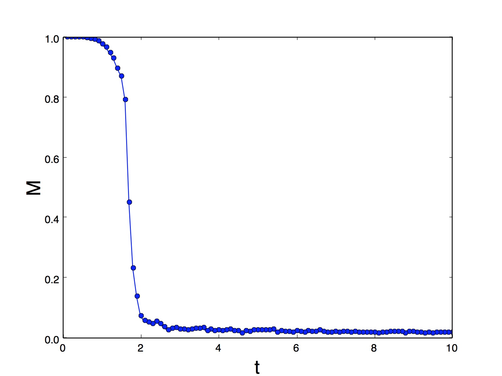
Figure 1: Magnetization $M$ vs. reduced temperature $t=\frac{k_{B}T}{J}$ obtained by using Metropolis Monte Carlo simulation for a square lattice with $40\times 40$ sites for the case 1. The error bars are smaller than size of the markers.

As shown by Enting, Guttmann and Jensenin Enting et al. (1994) at least the first 60 terms of low-temperature series expansion of thermodynamic functions are needed to have a physically consistent result. The critical temperature has been finally approximated as follows

$$\exp({-\frac{J}{k_{B}T_{c,SE}^{(1,\rm{square})}}})=x_{c,SE}^{(1,\rm{square})}=0.554075\pm 0.000015.$$

Also the calculation of the critical exponents $\beta$ and $\gamma$ associated to $M$ and $\chi$, respectively lead to the conclusion that the model belongs to the same universality class as spin-1/2 Ising model. Now, we apply the Metropolis Monte Carlo simulation on a 2D square lattice and examine these conclusions. Figure 1 shows the magnetization versus the reduced temperature, $t=\frac{k_{B}T}{J}$ for a square lattice with $40\times 40$ spins.

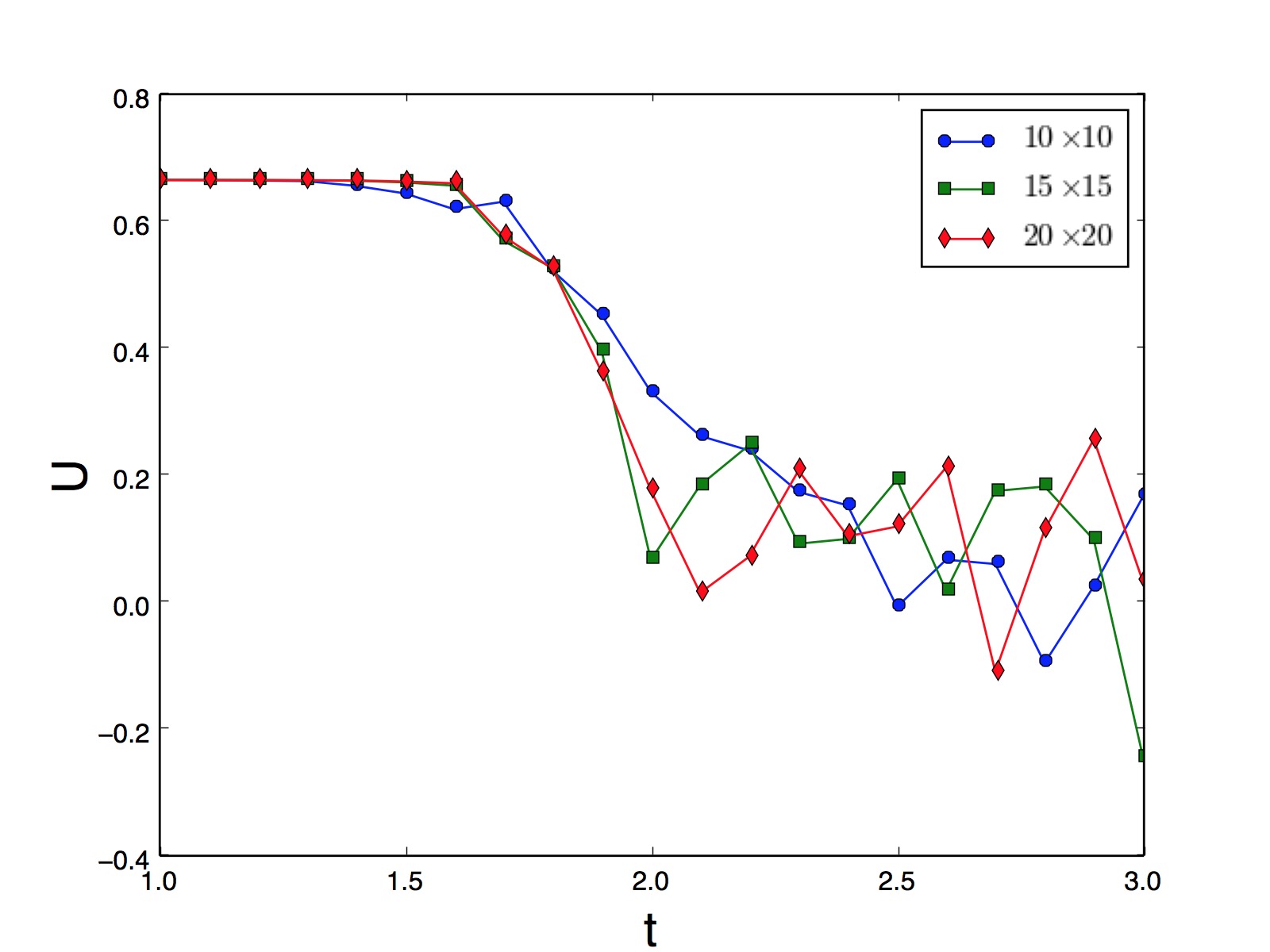
Figure 2: Binder Cumulant vs. $t=\frac{k_{B}T}{J}$ for different size lattices for Case 1. The error bars are smaller than size of the markers.

It shows that in the high temperature regime, system is in a disordered phase and the magnetization is zero, and for a reduced temperature $t=\frac{k_{B}T}{J}\simeq 1.7$ a critical phase transition occurs and the system evolves towards the ordered phase. Finally, for very low-temperatures the magnetization is close to one as expected.

The Binder cumulant defined as

$$U=1-\frac{<M^{4}>}{3<M^{2}>^{2}},$$ (26)

is an observational tool to estimate critical points. It turns out that the intersection of $U-T$ curves, for networks with different number of sites, gives the critical temperature of the lattice with a good accuracy Binder and Heermann (1997); Selke (2007). Figure 2 shows how we can use the Binder cumulant to determine the critical temperature considering three different size lattices. In this figure the Binder cumulants for three 2D square lattices with $5\times 5$, $10\times 10$, and $15\times 15$ sites are displayed. The intersection of the curves corresponds to the critical point given by

$$\frac{k_{B}T_{c,\rm{MC}}^{(1,\rm{square})}}{J}=1.70\pm 0.01.$$ (27)

This result is in the accordance with the critical temperature found from series expansion method given by (III.1).

In order to complete our discussion about this specific case we shall find some of the critical exponents of the model using the data we have obtained from simulation by the so called finite lattice method Newman (1999). Let us firstly evaluate the $\beta$ critical exponent. In order to calculate the $\beta$ exponent what is usually done is to plot $y=\ln M$ vs. $x=\ln l_{x}$. The slope of this graph is the $\beta$ exponent. Likewise the slope of $y=\ln\chi$ vs. $x=\ln l_{x}$ gives the $\gamma$ exponent. We eventually find

$$\beta=0.13\pm 0.01,$$ (28)

$$\gamma=1.78\pm 0.05.$$ (29)

These observations suggest that spin-1 Ising model governed by Hamiltonian (16) belongs to the same universality class of the spin-1/2 Ising model in agreement with series expansion method. In order to have an approximation of the critical temperature for a 3D cubic lattice we use again the Binder cumulant. The critical temperature is:

$$\frac{k_{B}T_{c,\rm{MC}}^{(1,\rm{cube})}}{J}=3.2\pm 0.1.$$ (30)

III.2 Case 2

In this subsection, we consider the Hamiltonian of the spin-1 Ising model given by (I) and we assume $J=L=0$. Therefore, the Hamiltonian of the system is:

$${\mathcal{H}_{\rm{Ising1}}^{(2)}}=-K\sum_{<ij>}s_{i}^{2}s_{j}^{2}-D\sum_{i=1}^{N}s_{i}^{2}-H\sum_{i=1}^{N}s_{i},$$ (31)

where $s_{i}=0$,$+1$,$-1$.

The Hamiltonian in the absence of an external magnetic field has been studied by Griffiths Griffiths (1967), who showed that the statistical mechanics of the spin-1 Ising model can be reduced to that of spin-1/2 Ising model. Although it would be possible in principle to solve this model with $H\neq 0$ using series expansion method, in this section we outline a very simple analytical solution not directly obtained with series expansion and we compare it with the results derived by means of Metropolis Monte Carlo technique simulations. We will prove that, by applying a simple transformation, the spin-1 Ising model is reduced to the spin-1/2 Ising model, with a constant exchange, but a temperature dependent external field Wu (1978). Before starting our discussion about the Hamiltonian (31) we make a very simple consideration. If we assume that $K=0$ the system does not exhibit any critical behavior because of the lack of a collective behavior in the system. Therefore, all the arguments in this subsection are valid only for $K\neq 0$ that marks the collective behavior in this case.

We consider a lattice of arbitrary dimensions and coordinate number $z$ described by the Hamiltonian (31). The partition function, $Z$ is defined by Yeomans (1993)

$$Z_{\rm{spin1}}=\sum_{s=0,+1,-1}e^{-\beta\mathcal{H}}$$ (32)

Substituting (31) in (32) and using the transformation $t_{i}=2s_{i}^{2}-1$ and some straightforward calculations we get

$$Z_{\rm{spin1}}^{(2)}=e^{N\beta C}\sum_{t_{i}=+1,-1}e^{R\sum_{i=1}^{N}t_{i}+Q\sum_{<ij>}t_{i}t_{j}},$$ (33)

where

$$C=\frac{1}{2\beta}\ln(2\cosh\beta H)+\frac{D}{2}+\frac{Kz}{8},$$ (34)

$$R=\frac{1}{2}\ln(2\cosh\beta H)+\frac{\beta D}{2}+\frac{\beta Kz}{4}$$ (35)

$$Q=\frac{\beta K}{4}.$$ (36)

Thus, according to the equation (33) the partition function of the spin-1 Ising model given by the Hamiltonian equation (31) with an appropriate transformation is reduced to that of the spin-1/2 Ising model with temperature dependent external field $\frac{R}{\beta}$ and temperature independent exchange interaction $\frac{Q}{\beta}$ times an exponential factor:

$$Z_{\rm{spin1}}^{(2)}=e^{N\beta C}\times Z_{\rm{spin1/2}}(\frac{R}{\beta},\frac{Q}{\beta}).$$ (37)

The Hamiltonian of the equivalent spin-1/2 Ising model with external field $\frac{R}{\beta}$ and exchange coefficient $\frac{Q}{\beta}$ is

$$\mathcal{H}_{\rm{spin1/2}}=-\frac{R}{\beta}\sum_{i=1}^{N}t_{i}-\frac{Q}{\beta}\sum_{<ij>}t_{i}t_{j}$$ (38)

So (33) and (38) show that spin-1 model with Hamiltonian (31) at temperatures less than the critical temperature exhibits the first order phase transition by crossing following surface:

$$\frac{R}{\beta}=0.$$ (39)

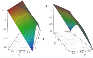
Figure 3: The surface $\frac{R}{\beta}=0$ in the $(T,D,H)$ space for $K=1$ in two views. We assume $k_{B}=1$ for simplicity.

Figure 3 displays the phase transition surface of the spin-1 Ising model governed by Hamiltonian (31) for $K=1$. So if we fix the temperature to a low enough value that is less than the critical temperature and change the external field $H$ in a wide enough range for appropriate values of $D$, there are two first-order phase transitions. Furthermore, it is clear that there is a maximum value of $D$ up to which the phase transition is possible; one can find this maximum value in the limit $T\to 0$, and $H\to 0$:

$$D_{\rm{max}}=-\frac{Kz}{2}.$$ (40)

Since we know the exact critical temperature of the spin-1/2 Ising model Onsager (1944) for the 2D square lattice, we can easily find the critical temperature for case 2 for such a lattice. The critical temperature of the 2D square lattice spin-1/2 Ising model with Hamiltonian (38) equation or equivalently for the spin-1 Ising model described by (31) is

$$T_{c}^{(2,\rm{square})}=\frac{K}{2k_{B}\ln(1+\sqrt{2})}$$ (41)

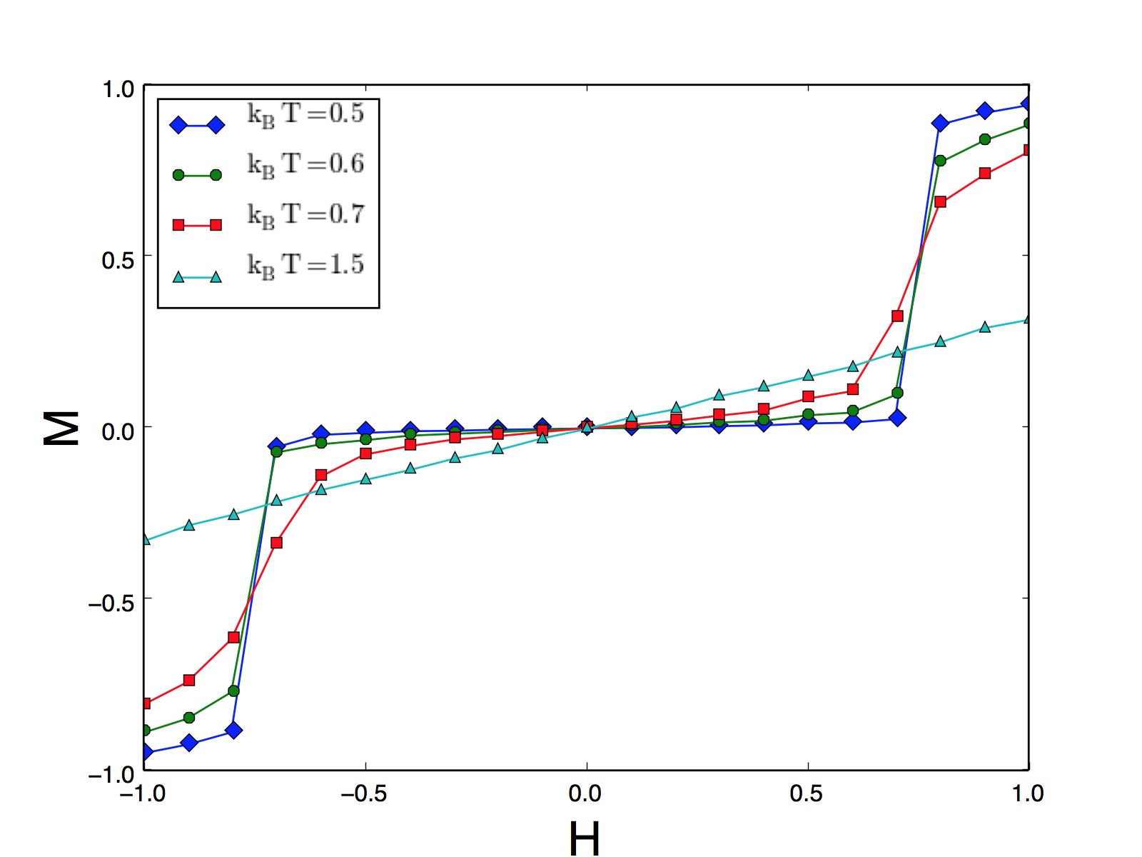
Figure 4: $M-H$ curves for case 2 with $D=-2.8$, and $K=1$ at different temperatures: $k_{B}T=0.5$, $k_{B}T=0.6$, $k_{B}T=0.7$, $k_{B}T=1.5$, for a $40\times 40$ square lattice obtained from Metropolis Monte Carlo simulation. The error bars are smaller than size of the markers.

We now perform Metropolis Monte Carlo simulation for 2D square lattice to compare the simulation results with the analytical calculation with special regard to the critical temperature. We set $K=1$, and use the suitable value for $D$, and change $H$, from $+1$ to $-1$ for different values of $T$. In Figure 4 the results for a $40\times 40$ 2D lattice are shown. The magnetization $M$ is plotted versus the external field, $H$ for different values of temperature. As it can be seen, for very low $T$, there are two jumps in the curve. One jump corresponds to a positive value of $H$, in which the magnetization jumps from $1$ to zero. Another jump occurs at a negative value of $H$, and in this case magnetization has a sudden variation from zero to $-1$. This result is conceptually is in accordance with our analytical solution. In fact, we have two first order phase transitions corresponding to the two values of $H$, where coefficient $\frac{R}{\beta}$ is zero. Moreover, the critical temperature can be estimated by plotting the susceptibility versus temperature; it turns out that

$$\frac{k_{B}T_{c,\rm{MC}}^{(2,\rm{square})}}{K}=0.57\pm 0.01$$ (42)

which agrees with the expression of the analytical critical temperature given by (41). The qualitative behavior of the 3D lattice system is very similar to the square lattice as we expect and the critical phase transition occurs at

$$\frac{k_{B}T_{c,\rm{MC}}^{(2,\rm{cube})}}{K}=1.20\pm 0.1.$$ (43)

III.3 Case 3

In this section we consider the Hamiltonian (I) with $K=0$:

$${\mathcal{H}_{\rm{Ising1}}^{(3)}}= -J\sum_{<ij>}s_{i}s_{j}-D\sum_{i=1}^{N}s_{i}^{2}-L\sum_{<ij>}(s_{i}^{2}s_{j}+s_{i}s_{j}^{2})$$

$$-H\sum_{i=1}^{N}s_{i},$$ (44)

and we apply mean-field approximation to obtain some physical quantities characterizing the model. More specifically, we get $F_{\rm{MF}}$ and, as a result, two self-consistent equations for mean-field magnetization $M$ and the thermal average of the square of the spin variable $\tau$:

$$F_{\rm{MF}}^{(3)}= -Nk_{B}T\times$$

$$\ln{\bigg{\{}1+2e^{\beta(D+LzM)}\cosh[\beta(zJM+H+Lz\tau)]\bigg{\}}}$$

$$+\frac{NJz}{2}M^{2}+NLzM\tau,$$ (45)

$$M=\frac{2e^{\beta(D+LzM)}\sinh[\beta(JzM+H+Lz\tau)]}{1+2e^{\beta(D+LzM)}\cosh[\beta(JzM+H+Lz\tau)]},$$

$$\tau=\frac{2e^{\beta(D+LzM)}\cosh[\beta(JzM+H+Lz\tau)]}{1+2e^{\beta(D+LzM)}\cosh[\beta(JzM+H+Lz\tau)]}.$$

One usual way to solve a system of nonlinear and transcendental algebraic equations like (III.3) and (III.3) is Newton’s method Ortega and Rheinboldt (2000). Eq.s (III.3) and (III.3) imply that no phase transitions are predicted by the mean-field theory for nonzero $L$. For instance, let us assume that in Hamiltonian (III.3) $L$ is positive and all the other coefficients vanish. When $T$ decreases, the system tends towards a configuration in which all the spins are up; for negative $L$ the system instead tends to a configuration with all spins down. Hence, $L$ plays a role similar to $H$. Furthermore, as should be expected, at high temperatures the system is in the disordered phase. In other words, the number of spin up, spin down and spin-less sites are equal, and consequently the magnetization is very small and $\tau$ is about $2/3\approx 0.67$. On the other hand, at very low-temperatures we have a completely ordered lattice with all sites spin up or down, i.e. $|M|\approx 1$. We emphasize that, for $L=0$, the model reduces to the Blum-Capel model Care (1993) and corresponding mean-field expressions for free energy, magnetization, and $\tau$ can be simply found from (III.3), (III.3) and (III.3). In particular, for $H=0$ we get

$$M=\frac{2e^{\beta D}\sinh{[\beta zJM]}}{1+2e^{\beta D}\cosh{[\beta zJM]}}.$$ (48)

Equation (48) enables us to calculate mean-field approximation for transition temperature, $T_{0}$; it’s enough to expand the expression on the right hand of (48) up to the first order of $M$. As $M\to 0$ we have $\sinh[\beta zJM]\to\beta zJM$ and $\cosh[\beta zJM]\to 1$, thus

$$zJ\beta_{0}=1+\frac{1}{2}e^{-\beta_{0}D},$$ (49)

where $\beta_{0}=\frac{1}{k_{B}T_{0}}$. Equation (49) determines the curve of phase transition in phase diagram of Blum-Capel model at $H=0$ plane, however up to now we do not know the type of phase transition occurring at $T_{0}$. Using (III.3) we write down the first few terms of series expansion of the zero external field free energy around $M=0$:

$$F_{\rm{MF}}(H=0)\simeq a_{0}+a_{2}M^{2}+a_{4}M^{4},$$ (50)

with

$$a_{0}=-Nk_{B}T\ln{(1+2e^{\beta D})},$$ (51)

$$a_{2}=\frac{zJ}{2}[1-\beta zJ\frac{2e^{\beta D}}{1+2e^{\beta D}}],$$ (52)

$$a_{4}=\frac{zJ}{24}{(\beta zJ)}^{3}\frac{2e^{\beta D}}{1+2e^{\beta D}}[\frac{6e^{\beta D}}{1+2e^{\beta D}}-1].$$ (53)

The essential condition for having a critical phase transition according to Landau theory is Yeomans (1993)

$$a_{2}=0,\ a_{4}>0.$$ (54)

Hence, to have a critical phase transition we get according to mean-field theory

$$D>-zJ\frac{\ln{4}}{3}.$$ (55)

In addition, at the tricritical ($\rm{tc}$) point where the three phases predicted by the classical spin-1 Ising model become critical simultaneously we must have

$$a_{2}=0,\ a_{4}=0.$$ (56)

Then, the $\rm{tc}$ point is determined by

$$\beta_{\rm{tc},\rm{MF}}^{(3)}zJ=3,\ D_{\rm{tc},\rm{MF}}^{(3)}=-zJ\frac{\ln{4}}{3}.$$ (57)

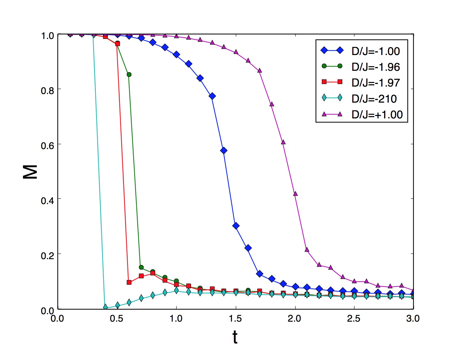
Figure 5: Absolute magnetization $M$ vs. reduced temperature $t=k_{B}T/J$ for different values of $D$ for a 2D square lattice with $20\times 20$ sites described by the Blum-Capel Hamiltonian in zero external field according to Metropolis Monte Carlo simulation for $D/J=1.00$, $D/J=-1.00$, $D/J=-1.96$, $D/J=-1.97$ and $D/J=-2.10$. The critical phase transition becomes first-order at $D_{\rm{tc,MC}}^{(3,\rm{square})}/J=-1.96\pm 0.01$, and $t_{\rm{tc,MC}}^{(3,\rm{square})}=0.64\pm 0.01$. The error bars are smaller than size of the markers.

Mean-field solution in general is not the exact solution but only approximated because it neglects the effect of dimensionality. The results of mean-field calculations become more precise when the dimensionality of the system becomes larger and the mean-field predictions, like for example the critical exponents, become exact if the dimensionality of the system is equal or higher than the upper critical dimension, $d_{\rm{up}}$, which is given by Als-Nielsen and J. Birgeneau (1977)

$$d_{\rm{up}}=\frac{(\gamma+2\beta)}{\nu}.$$ (58)

Mean-field usually gives good predictions for the phase diagrams of the 3D systems Yeomans (1993). In this respect, the interesting example is a 3D system like a cubic lattice at the $\rm{tc}$ point. At the $\rm{tc}$ point we have the following critical exponents Als-Nielsen and J. Birgeneau (1977)

$$\beta_{\rm{tc}}=\frac{1}{4},\ \nu_{\rm{tc}}=\frac{1}{2},\ \gamma_{\rm{tc}}=1,$$ (59)

(58) and (59) lead to

$$d_{\rm{up}}=3.$$ (60)

It means that at the $\rm{tc}$ point, mean-field theory provides a very good description of the model in 3D lattices in terms of critical exponents. So for the spin-1 3D Ising model, which is described by the Hamiltonian (III.3), around the $\rm{tc}$ point, for zero external field and $L=0$ the critical exponents are the ones given by (59).

Now we use the Metropolis Monte Carlo technique to investigate the behavior of 2D square and 3D cubic lattices defined by the Hamiltonian (III.3) and compare the results with those of mean-field theory. Figure 5 shows the absolute magnetization versus reduced temperature for different values of $D$ obtained by Metropolis Monte Carlo simulation for a 2D square lattice. It agrees qualitatively with mean-field but obviously leads to different values for the $\rm{tc}$ point:

$$\frac{D_{\rm{tc},\rm{MC}}^{(3,\rm{square})}}{J} =-1.96\pm 0.01,$$

$$\frac{k_{B}T_{\rm{tc},\rm{MC}}^{(3,\rm{square})}}{J} =0.64\pm 0.01.$$ (61)

We have already seen that mean-field approximation suggests that the spin-1 Ising model governed by (III.3) does not exhibit any phase transitions when $L$ is nonzero.Interestingly, Metropolis Monte Carlo simulation that is a more accurate method confirms this result. For instance, Figure 6 proves the non-existence of the phase transition for a 2D square lattice with $20\times 20$ spins in the case in which only $L$ is non-zero. For a 3D cubic lattice the system behavior is similar and $\rm{tc}$ point is given by

$$\frac{D_{\rm{tc},\rm{MC}}^{(3,\rm{cube})}}{J} =-2.86\pm 0.01,$$

$$\frac{T_{\rm{tc},\rm{MC}}^{(3,\rm{cube})}}{J} =1.4\pm 0.1.$$ (62)

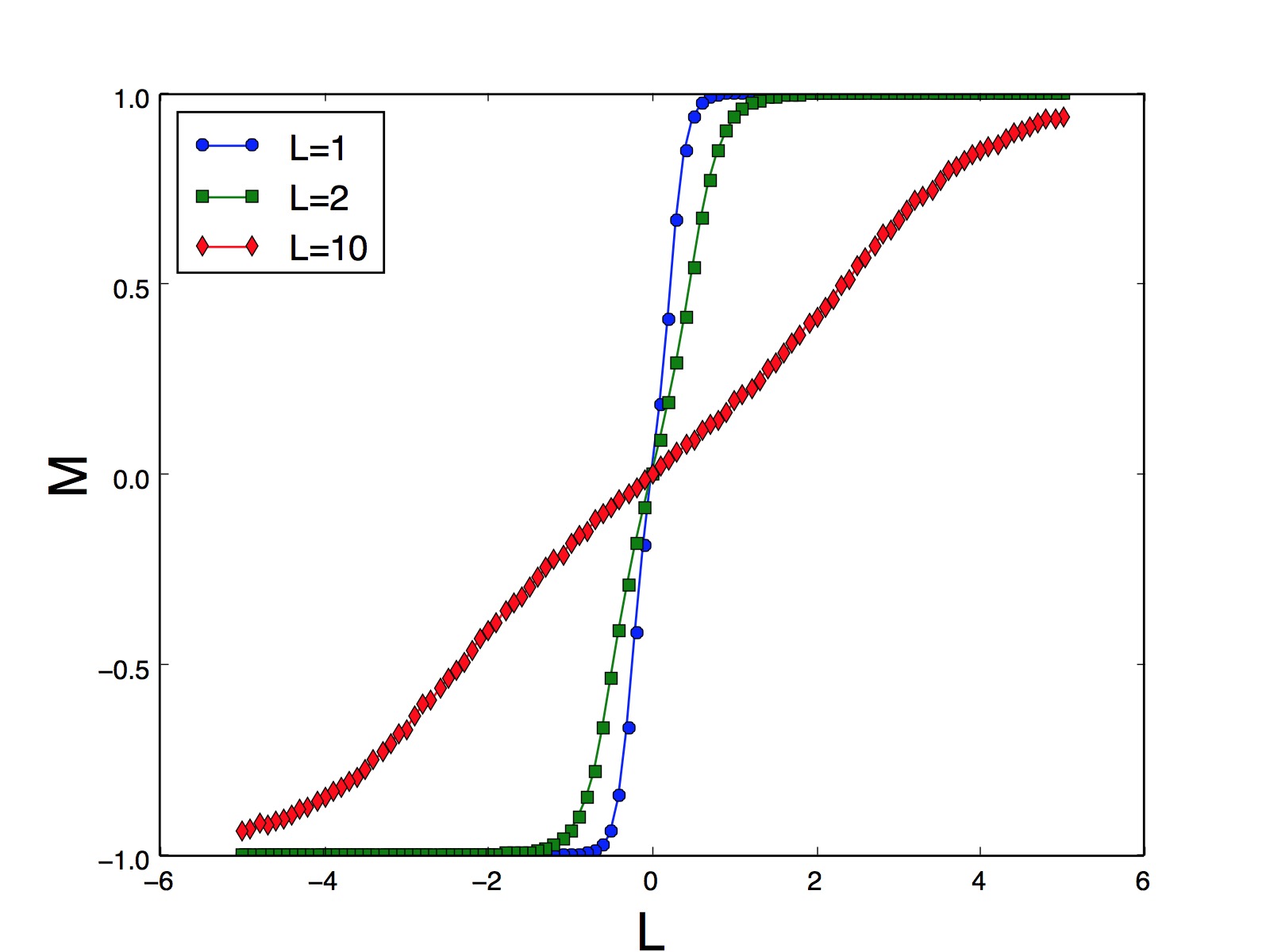
Figure 6: Magnetization as a function of L plots obtained from Metropolis Monte Carlo simulation for the spin-1 Ising model defined by Hamiltonian (III.3) for a $20\times 20$ square lattice with $H=D=J=0$ for $k_{B}T/L=1.0$, $k_{B}T/L=2.0$, Bottom: $k_{B}T/L=10.0$, which indicates that no phase transition takes place. Error bars are smaller than size of the markers.

III.4 Case 4

As another specific case we consider the following spin-1 Ising model

$${\mathcal{H}_{\rm{Ising1}}^{(4)}}=-J\sum_{<ij>}s_{i}s_{j}-K\sum_{<ij>}s_{i}^{2}s_{j}^{2}-D\sum_{i=1}^{N}s_{i}^{2}.$$

First note that this Hamiltonian is equivalent to the Ising spin-1/2 lattice gas with following Hamiltonian:

$$\mathcal{H}_{\rm{lg}}=-J\sum_{<ij>}s_{i}s_{j}t_{i}t_{j}-K\sum_{<ij>}t_{i}t_{j}-D\sum_{i=1}^{N}t_{i},$$

where $s_{i}=\pm 1$ and $t_{i}=0,1$ and the subscript $lg$ denotes lattice gas. Before we prove this equivalence let us discuss about the Hamiltonian (III.4) shortly. For simplicity, we assume that we have a 2D square lattice with $N$ sites. According to the spin-1/2 Ising lattice gas model each site can be occupied with a particle or it can be a vacancy. If site $i$ is occupied, the variable $t_{i}$ is one, otherwise it will be zero. In the Hamiltonian (III.4) the first term proportional to $J$ expresses an exchange interaction between two neighbor sites if and only if both are occupied and the amount and sign of this interaction depend on spin variables of these two occupied sites. The second term of $\mathcal{H}_{\rm{lg}}$ proportional to $K$ is the interaction energy between a pair of filled neighbors regardless of their spins and the last term proportional to $D$ is a spin independent effect of some external field with occupied sites with $D$ playing the role of this field. Now we are ready to prove the equivalence of $\mathcal{H}_{\rm{Ising1}}^{(4)}$ given by (III.4) and $\mathcal{H}_{\rm{lg}}$ given by (III.4). To do it we start from (III.4) and impose the following transformation

$$r_{i}=t_{i}s_{i}$$ (65)

Equation (65) illustrates that $r_{i}$ can be $+1$, $-1$, or $0$. Obviously $r_{i}^{2}$ only has two possible values: $+1$, or $0$. So in the two last terms of (III.4) we can substitute $t_{i}$ with $r_{i}^{2}$. Thus $\mathcal{H}_{\rm{lg}}$ in terms of new spin variable $r_{i}$ is

$$\mathcal{H}_{\rm{lg}}=-J\sum_{<ij>}r_{i}r_{j}-K\sum_{<ij>}r_{i}^{2}r_{j}^{2}-D\sum_{i=1}^{N}r_{i}^{2}.$$ (66)

Thus Hamiltonians (III.4) and (III.4) are equivalent and share the same physics. This equivalence is conceptually trivial, because spin-1 model can be considered as a spin-1/2 model with vacancies but the underlying physics is interesting. Regarding this point, historically Blume, Emery, and Griffiths suggested the Hamiltonian (III.4) as a spin-1 lattice model to describe a mixture of non-magnetic $(s=0)$ and magnetic $(s=\pm 1)$ components Blume et al. (1971). The model was originally inspired by the experimental observation that the continuous superfluid transition in $\rm{He}^{3}$ with $\rm{He}^{4}$ impurity becomes a first order transition into normal and superfluid phase separation above some critical $\rm{He}^{3}$ concentration.

Table 2: Metropolis Monte Carlo simulation result for $T_{\rm{tc}}$ and $D_{\rm{tc}}$ for different values of $K$ for a $20\times 20$ 2D spin square lattice governed by the Hamiltonian (III.4).

$K/J$	$k_{B}T_{\rm{tc}}/J$	$D_{\rm{tc}}/J$
0.00	0.64	-1.96
0.10	0.68	-2.16
0.20	0.75	-2.36
0.30	0.82	-2.56
0.40	0.85	-2.75
0.50	0.92	-2.96
0.60	0.97	-3.16

Blume, Emery and Griffiths have found the mean-field solution and have determined the approximated phase diagram and the $\rm{tc}$ of the model. Since we have found that Metropolis Monte Carlo results qualitatively agree with the mean-field solution, e.g. phase diagrams obtained from the two methods are similar, in Table 2 we present the Metropolis Monte Carlo simulation results for the tc temperature $T_{\rm{tc}}$ and the tc crystal field of strength $D_{\rm{tc}}$ for a 2D square lattice. These results show that with increasing $K$ there is an increase of $T_{\rm{tc}}$ and a negative increase of $D_{\rm{tc}}$.

III.5 Case 5: long-range Ising spin-1 model

Long-range interaction that are typical of statistical mechanical systems may affect the critical behavior of the corresponding models Campa et al. (2009). Regarding this, in this section we deal with the 2D spin-1 Ising model with long-range spin interactions. We investigate the effect of this further interaction using Metropolis Monte Carlo simulation comparing the results with the ones of the corresponding 2D spin-1/2 Ising model in the presence of the same interaction. In analogy with long-range spin-1/2 Ising model Balog et al. (2014); Fisher et al. (1972) we define the long-range Hamiltonian for spin-1 Ising model as follows

$$\mathcal{H}_{\rm{lr}}^{(5)}=-\sum_{ij}\frac{J}{r_{ij}^{d+\sigma}}s_{i}s_{j},$$ (67)

where $s_{i}=0$, $1$, or $-1$, $d$ is the lattice dimensionality, $\sigma$ is the phenomenological parameter which determines the interaction strength, $r_{ij}$ is the distance between a couple of spins labeled by the indices $i$ and $j$, and the subscript $lr$ denotes long range. Explicitly, in the Metropolis algorithm if the flipped spin is at position $(x,y)$ we have

$$r_{ij}=\sqrt{{(x-i)}^{2}+{(y-j)}^{2}}.$$ (68)

In this analysis we limit ourselves to ferromagnetic materials, i.e. $J>0$. Notice that for spin-1/2 Ising model the Hamiltonian (67) has the same expression but $s_{i}=1$, or $-1$.

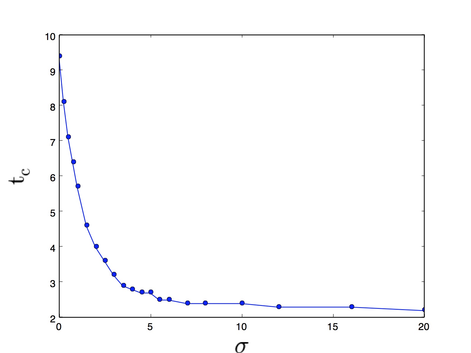
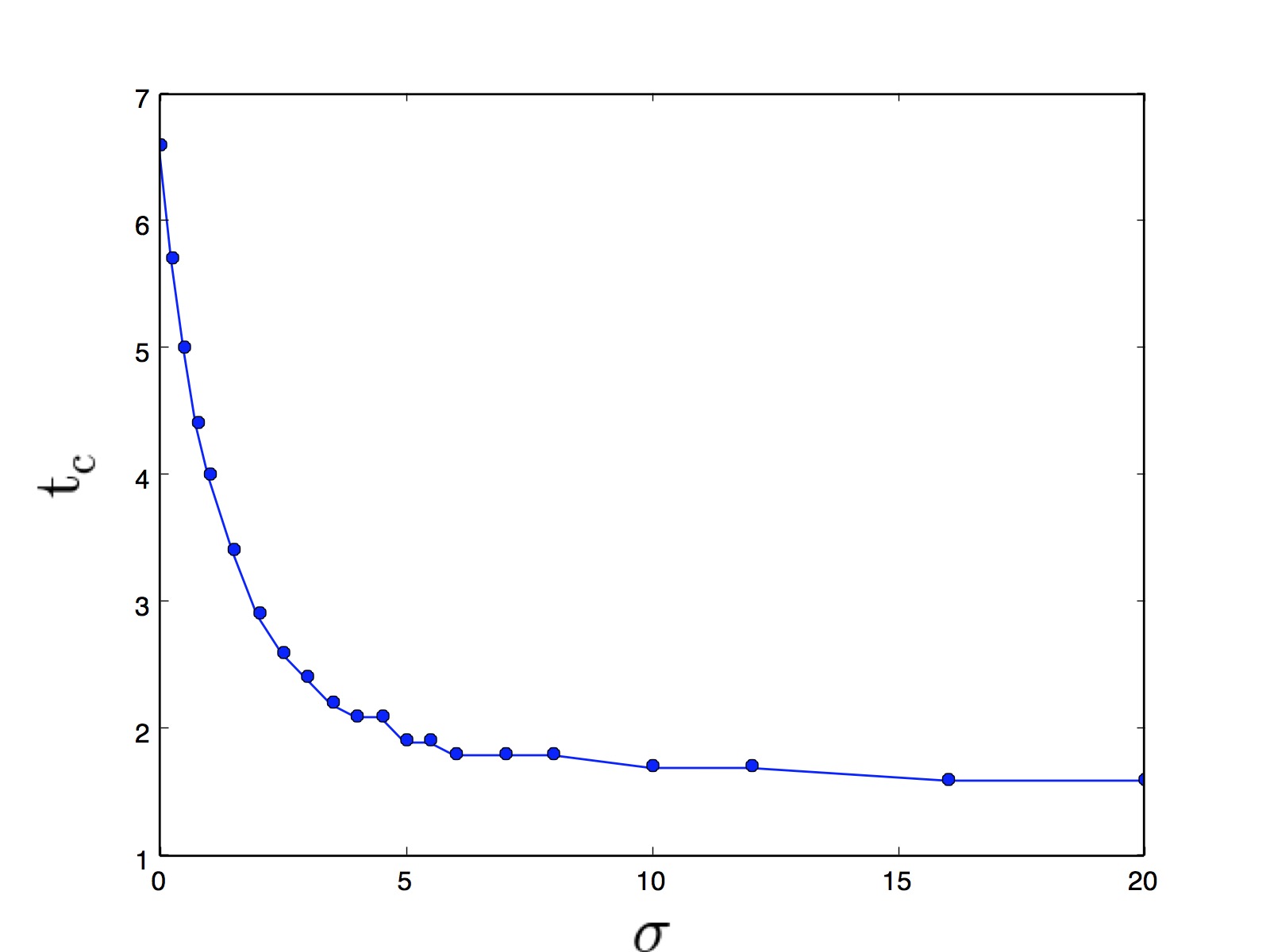
Figure 7: $t_{c}=\frac{k_{B}T_{c}}{J}$ as a function of $\sigma$ for the long-range interaction Ising model Top: spin-1/2, Bottom: spin-1 for a square lattice with $40\times 40$ sites described by Hamiltonian (67) with $R=7$ obtained from Metropolis Monte Carlo simulation. Error bars are smaller than size of the markers.

On the basis of this numerical simulation we can investigate the dependence of the critical temperature on $\sigma$. We do the Metropolis Monte Carlo simulation for different values of parameter $\sigma$, considering the long-range interaction and assuming that each spin interacts with other spins which their distance is equal or less than some radius $R$. In other words the summation in the Hamiltonian (67) is carried out over all spins, which are in the circle of radius $R$ around the flipped spin in each step of Metropolis algorithm. It means that in the algorithm $r_{ij}<R$. Figure 7 shows the result for $R=7$. As we expect the critical temperature of the model decreases with parameter $\sigma$. The dependence of critical temperature on parameter $\sigma$, basing upon the results of numerical modelling of the least squares for spin-1/2 is given by

$$\frac{k_{B}T_{c,\rm{spin-1/2}}^{\rm{lr}}}{J}=2.3+6.9e^{-0.7\sigma}.$$ (69)

Similarly for spin-1 model we get:

$$\frac{k_{B}T_{c,\rm{spin-1}}^{\rm{lr}}}{J}=1.7+4.7e^{-0.7\sigma}.$$ (70)

So in both cases we have

$$T_{c}=a+be^{-c\sigma},$$ (71)

where $a$ is the critical temperature of the short-range model and $c\approx 0.7$.

IV Conclusion

In the present work we studied the classical spin-1 Ising model using different analytical and numerical methods such as mean-field theory, series expansions and Monte Carlo simulation to investigate some critical properties of the model like critical temperature and critical exponents for 1D chain, 2D square lattice, and 3D cubic lattice. We have found that, albeit some similarities with the critical behavior of the classical spin-1/2 Ising model, because of the presence in the Hamiltonian of the spin-1 model of more terms, i.e. more different types of interactions between spin pairs, the critical properties of this model are much richer and more variegated with respect to the ones of the corresponding spin-1/2 Ising model.

We have used mean-field theory that represents a strong mathematical tool to study the physics of the model in some special cases. We have found that, for 3D lattices near the tricritical point, the critical properties of the model can be described by mean-field theory. In particular, we have found that the critical exponents around the tricritical point calculated via the mean-field approximation are confirmed by Monte Carlo simulations. On the other hand, the mean-field results for 2D lattices are only qualitatively but not quantitatively correct as highlighted by Monte Carlo simulation. The simulation results obtained for 2D square and 3D cubic lattices can be easily extended to other types of lattices.

We have shown that, for a special case of the spin-1 Ising model where the bilinear and the bicubic terms are set equal to zero, it is possible to write the corresponding partition function in arbitrary dimensions as the one of the spin-1/2 Ising model in agreement with our Monte Carlo simulation. Finally, we have investigated the long-range spin-1 Ising model Hamiltonian by including in the Hamiltonian a long-range interaction term in analogy with what was carried out for spin-1/2 Ising model determining the dependence of the critical temperature of the two models on the strength of this interaction.

References

- Ising (1925) E. Ising, Zeitschrift für Physik 31, 253 (1925).
- Brush (1967) S. G. Brush, Rev. Mod. Phys. 39, 883 (1967).
- Peierls and Born (1936) R. Peierls and M. Born, Proceedings of the Cambridge Philosophical Society 32, 477 (1936).
- Onsager (1944) L. Onsager, Phys. Rev. 65, 117 (1944).
- Baxter (2012) R. J. Baxter, Journal of Statistical Physics 149, 1164 (2012).
- Yang (1952) C. N. Yang, Phys. Rev. 85, 808 (1952).
- Yeomans (1993) J. M. Yeomans, Statistical Mechanics of Phase Transitions (Oxford University Press, Oxford, 1993).
- Newman (1999) M. E. Newman, Monte Carlo Methods in Statistical Physics (Oxford University Press, New York, 1999).
- Sonsin et al. (2015) A. F. Sonsin, M. R. Cortes, D. R. Nunes, J. V. Gomes, and R. S. Costa, Journal of Physics: Conference Series 630, 012057 (2015).
- Kaneyoshi and Mielnicki (1990) T. Kaneyoshi and J. Mielnicki, Journal of Physics: Condensed Matter 2, 8773 (1990).
- Benyoussef et al. (1987) A. Benyoussef, T. Biaz, M. Saber, and M. Touzani, Journal of Physics C: Solid State Physics 20, 5349 (1987).
- Kaneyoshi (1987) T. Kaneyoshi, Journal of the Physical Society of Japan 56, 933 (1987).
- Kaneyoshi (1988) T. Kaneyoshi, Journal of Physics C: Solid State Physics 21, L679 (1988).
- Boccara et al. (1989) N. Boccara, A. Elkenz, and M. Saber, Journal of Physics: Condensed Matter 1, 5721 (1989).
- Kaneyoshi (1986) T. Kaneyoshi, Journal of Physics C: Solid State Physics 19, L557 (1986).
- Tucker (1989) J. W. Tucker, Journal of Physics: Condensed Matter 1, 485 (1989).
- Jurčišinová and Jurčišin (2016) E. Jurčišinová and M. Jurčišin, Physica A: Statistical Mechanics and its Applications 461, 554 (2016).
- Blume et al. (1971) M. Blume, V. J. Emery, and R. B. Griffiths, Phys. Rev. A 4, 1071 (1971).
- Huang and Beale (1988) K. Huang and P. Beale, Statistical Mechanics (Wiley, New York, 1988).
- Enting et al. (1994) I. G. Enting, A. J. Guttmann, and I. Jensen, Journal of Physics A: Mathematical and General 27, 6987 (1994).
- Fox and Guttmann (1973) P. F. Fox and A. J. Guttmann, Journal of Physics C: Solid State Physics 6, 913 (1973).
- Saul et al. (1974) D. M. Saul, M. Wortis, and D. Stauffer, Phys. Rev. B 9, 4964 (1974).
- Yeomans and E. Fisher (1981) J. Yeomans and M. E. Fisher, Phys. Rev. B 24 (1981), 10.1103/PhysRevB.24.2825.
- K. Jain (1980) A. K. Jain, Phys. Rev. B 22 (1980), 10.1103/PhysRevB.22.445.
- Care (1993) C. M. Care, Journal of Physics A: Mathematical and General 26, 1481 (1993).
- Binder and Heermann (1997) K. Binder and D. Heermann, Monte Carlo Simulation in Statistical Physics (Springer, Berlin, 1997).
- Selke (2007) W. Selke, Journal of Statistical Mechanics: Theory and Experiment 2007, P04008 (2007).
- Griffiths (1967) R. B. Griffiths, Physica 33, 689 (1967).
- Wu (1978) F. Wu, Chinese Journal of Physics 16, 153 (1978).
- Ortega and Rheinboldt (2000) J. Ortega and W. Rheinboldt, Iterative Solution of Nonlinear Equations in Several Variables (SIAM Publications Classics in Appl. Math, Philadelphia, 2000).
- Als-Nielsen and J. Birgeneau (1977) J. Als-Nielsen and R. J. Birgeneau, American Journal of Physics - AMER J PHYS 45, 554 (1977).
- Campa et al. (2009) A. Campa, T. Dauxois, and S. Ruffo, Physics Reports 480, 57 (2009).
- Balog et al. (2014) I. Balog, G. Tarjus, and M. Tissier, Journal of Statistical Mechanics: Theory and Experiment 2014, P10017 (2014).
- Fisher et al. (1972) M. E. Fisher, S.-k. Ma, and B. G. Nickel, Phys. Rev. Lett. 29, 917 (1972).