Planar Distance Oracles with Better Time-Space Tradeoffs

Abstract

In a recent breakthrough, Charalampopoulos, Gawrychowski, Mozes, and Weimann [9] showed that exact distance queries on planar graphs could be answered in $n^{o(1)}$ time by a data structure occupying $n^{1+o(1)}$ space, i.e., up to $o(1)$ terms, optimal exponents in time (0) and space (1) can be achieved simultaneously. Their distance query algorithm is recursive: it makes successive calls to a point-location algorithm for planar Voronoi diagrams, which involves many recursive distance queries. The depth of this recursion is non-constant and the branching factor logarithmic, leading to $(\log n)^{\omega(1)}=n^{o(1)}$ query times.

In this paper we present a new way to do point-location in planar Voronoi diagrams, which leads to a new exact distance oracle. At the two extremes of our space-time tradeoff curve we can achieve either

$$\begin{array}[]{lll}\mbox{$n^{1+o(1)}$ space }&\mbox{and}&\mbox{ $\log^{2+o(1)}n$ query time, or }\\ &&\\ \mbox{$n\log^{2+o(1)}n$ space }&\mbox{and}&\mbox{$n^{o(1)}$ query time.}\\ \end{array}$$

All previous oracles with $\tilde{O}(1)$ query time occupy space $n^{1+\Omega(1)}$, and all previous oracles with space $\tilde{O}(n)$ answer queries in $n^{\Omega(1)}$ time.

1 Introduction

A distance oracle is a data structure that answers distance queries (or approximate distance queries) w.r.t. some underlying graph or metric space. On general graphs there are many well known distance oracles that pit space against multiplicative approximation [41], space against mixed multiplicative/additive approximation [35, 1], and, in sparse graphs, space against query time [2, 39]. Refer to Sommer [38] for a survey on distance oracles.

Whereas approximation seems to be a necessary ingredient to achieve any reasonable space/query time on general graphs, structured graph classes may admit exact distance oracles with attractive time-space tradeoffs. In this paper we continue a long line of work [3, 15, 10, 18, 28, 42, 33, 7, 32, 11, 20, 9] focused on exact distance oracles for weighted, directed planar graphs.

History.

Between 1996-2012, work of Arikati et al. [3], Djidjev [15], Chen and Xu [10], Fakcharoenphol and Rao [18], Klein [28], Wulff-Nilsen [42], Nussbaum [33], Cabello [7], and Mozes and Sommer [32] achieved space $\tilde{O}(S)$ and query time $\tilde{O}(n/\sqrt{S})$, for various ranges of $S$ that ultimately covered the full range $[n,n^{2}]$.

In 2017, Cabello [8] introduced planar Voronoi diagrams as a tool for solving metric problems in planar graphs, such as diameter and sum-of-distances. This idea was incorporated into new planar distance oracles, leading to $\tilde{O}(n^{5/2}/S^{3/2})$ query time [11] for $S\in[n^{3/2},n^{5/3}]$ and $\tilde{O}(n^{3/2}/S)$ query time [20] for $S\in[n,n^{3/2}]$. Finally, in a major breakthrough Charalampopoulos, Gawrychowski, Mozes, and Weimann [9] demonstrated that up to $n^{o(1)}$ factors, there is no tradeoff between space and query time, i.e., space $n^{1+o(1)}$ and query time $n^{o(1)}$ can be achieved simultaneously. In more detail, they proved that space $O(n^{4/3}\sqrt{\log n})$ allows for query time $O(\log^{2}n)$, space $\tilde{O}(n^{1+\epsilon})$ allows for query time $O(\log n)^{1/\epsilon-1}$, and space $O(n\log^{2+1/\epsilon}n)$ allows for query time $O(n^{2\epsilon})$.

The Charalampopoulos et al. structure is based on a hierarchical $\vec{r}$-decomposition of the graph, $\vec{r}=(n,n^{(m-1)/m},\ldots,n^{1/m})$. (See Section 2.) Given $u,v$, it iteratively finds the last boundary vertex $u_{i}$ on the shortest $u$-$v$ path that lies on the boundary of the level-$i$ region containing $u$. Given $u_{i-1}$, finding $u_{i}$ amounts to solving a point location problem on an external Voronoi diagram, i.e., a Voronoi diagram of the complement of a region in the hierarchy. Each point location query is solved via a kind of binary search, and each step of the binary search involves 3 recursive distance queries that begin at a “higher” level in the hierarchy. This leads to a tradeoff between space $\tilde{O}(n^{1+1/m})$ and query time $O(\log n)^{m-1}$.

See Table 1 for a summary of the space-time tradeoffs exact and approximate planar distance oracles.

Reference	Space	Query Time
Arikati, Chen, Chew Das, Smid & Zaroliagis 1996	$S\in[n^{3/2},n^{2}]$	$O\mathopen{}\left(\frac{n^{2}}{S}\right)\mathclose{}$
Djidjev 1996	$S\in[n,n^{2}]$	$O\mathopen{}\left(\frac{n^{2}}{S}\right)\mathclose{}$
	$S\in[n^{4/3},n^{3/2}]$	$O\mathopen{}\left(\frac{n}{\sqrt{S}}\log n\right)\mathclose{}$
Chen & Xu 2000	$S\in[n^{4/3},n^{2}]$	$O\mathopen{}\left(\frac{n}{\sqrt{S}}\log\mathopen{}\left(\frac{n}{\sqrt{S}}\right)\mathclose{}\right)\mathclose{}$
Fakcharoenphol & Rao 2006	$O(n\log n)$	$O(\sqrt{n}\log^{2}n)$
Wulff-Nilsen 2010	$O(n^{2}\frac{\log^{4}\log n}{\log n})$	$O(1)$
Nussbaum 2011	$O(n)$	$O(n^{1/2+\epsilon})$
	$S\in[n^{4/3},n^{2}]$	$O\mathopen{}\left(\frac{n}{\sqrt{S}}\right)\mathclose{}$
Cabello 2012	$S\in[n^{4/3}\log^{1/3}n,n^{2}]$	$O\mathopen{}\left(\frac{n}{\sqrt{S}}\log^{3/2}n\right)\mathclose{}$
Mozes & Sommer 2012	$S\in[n\log\log n,n^{2}]$	$O\mathopen{}\left(\frac{n}{\sqrt{S}}\log^{2}n\log^{3/2}\log n\right)\mathclose{}$
	$O(n)$	$O(n^{1/2+\epsilon})$
Cohen-Addad, Dahlgaard & Wulff-Nilsen 2017	$S\in[n^{3/2},n^{5/3}]$	$O\mathopen{}\left(\frac{n^{5/2}}{S^{3/2}}\log n\right)\mathclose{}$
Gawrychowski, Mozes, Weimann & Wulff-Nilsen 2018	$\tilde{O}(S)$ for $S\in[n,n^{3/2}]$	$\tilde{O}\mathopen{}\left(\frac{n^{3/2}}{S}\right)\mathclose{}$
Charalampopoulos, Gawrychowski, Mozes & Weimann 2019	$O(n^{4/3}\sqrt{\log n})$	$O(\log^{2}n)$
	$n^{1+o(1)}$	$n^{o(1)}$
new 2020	$n^{1+o(1)}$	$\log^{2+o(1)}n$
	$n\log^{2+o(1)}n$	$n^{o(1)}$
$(1+\epsilon)$-Approx. Oracles	Space	Query Time
Thorup 2001	$O(n\epsilon^{-1}\log^{2}n)$	$O(\log\log n+\epsilon^{-1})$
	$O(n\epsilon^{-1}\log n)$	$O(\epsilon^{-1})$ (Undir.)
Klein 2002	$O(n(\log n+\epsilon^{-1}\log\epsilon^{-1}))$	$O(\epsilon^{-1})$ (Undir.)
Kawarabayashi, Klein, & Sommer 2011	$O(n)$	$O(\epsilon^{-2}\log^{2}n)$ (Undir.)
Kawarabayashi, Sommer, & Thorup 2013	$\overline{O}(n\log n)$	$\overline{O}(\epsilon^{-1})$ (Undir.)
	$\overline{O}(n)$	$\overline{O}(\epsilon^{-1})$    (Undir.,Unweight.)

Table 1: Space-query time tradeoffs for exact and approximate planar distance oracles. $\overline{O}$ hides $\log(\epsilon^{-1}\log n)$ factors.

New Results.

In this paper we develop a more direct and more efficient way to do point location in external Voronoi diagrams. It uses a new persistent data structure for maintaining sets of non-crossing systems of chords, which are paths that begin and end at the boundary vertices of a region, but are internally vertex disjoint from the region. By applying this point location method in the framework of Charalampopoulos et al. [9], we obtain a better time-space tradeoff, which is most noticeable at the “extremes” when $\tilde{O}(n)$ space or $\tilde{O}(1)$ query time is prioritized.

Theorem 1.1.

Let $G$ be an $n$-vertex weighted planar digraph with no negative cycles, and let $\kappa,m\geq 1$ be parameters. A distance oracle occupying space $O(m\kappa n^{1+1/m+1/\kappa})$ can be constructed in $\tilde{O}(n^{3/2+1/m}+n^{1+1/m+1/\kappa})$ time that answers exact distance queries in $O(2^{m}\kappa\log^{2}n\log\log n)$ time. At the two extremes of the space-time tradeoff curve, we can construct oracles in $n^{3/2+o(1)}$ time with either

• $n^{1+o(1)}$ space and $\log^{2+o(1)}n$ query time, or

• $n\log^{2+o(1)}n$ space and $n^{o(1)}$ query time.

Our new point-location routine suffices to get the query time down to $O(\log^{3}n)$. In order to reduce it further to $O(\log^{2+o(1)}n)$, we develop a new dynamic tree data structure based on Euler-Tour trees [23] with $O(\kappa n^{1/\kappa})$ update time and $O(\kappa)$ query time. This allows us to generate MSSP (multiple-source shortest paths) structures with a similar space-query tradeoff, specifically, $O(\kappa n^{1+1/\kappa})$ space and $O(\kappa\log\log n)$ query time. Our MSSP construction follows Klein [28] (see also [20]), but uses our new dynamic tree in lieu of Sleator and Tarjan’s Link-Cut trees [37], and uses persistent arrays [12] in lieu of [16] to make the data structure persistent.

Organization.

In Section 2 we review background on planar embeddings, planar separators, multiple-source shortest paths, and weighted Voronoi diagrams. In Section 3 we introduce key parts of the data structure and describe the query algorithm, assuming a certain point location problem can be solved. Section 4 introduces several more components of the data structure, and shows how they can be applied to solve this particular point location problem in near-logarithmic time. The space and query-time claims of Theorem 1.1 are proved in Section 5. The construction time claims of Theorem 1.1 are proved in Appendix C. Appendix A gives the MSSP construction based on Euler Tour trees. Appendix B explains how to remove a simplifying assumption made throughout the paper, that the boundary vertices of every region in the $\vec{r}$-decomposition lie on a single hole, which is bounded by a simple cycle.

2 Preliminaries

2.1 The Graph and Its Embedding

A weighted planar graph $G=(V,E,\ell)$ is represented by an abstract embedding: for each $v\in V(G)$ we list the edges incident to $v$ according to a clockwise order around $v$. We assume the graph has no negative weight cycles and further assume the following, without loss of generality.

• All the edge-weights can be made non-negative ($\ell:E\rightarrow\mathbb{R}_{\geq 0}$) [24]. Furthermore, via randomized or deterministic perturbation [17], we can assume there are no zero weight edges, and that shortest paths are unique in any subgraph of $G$.

• The graph is connected and triangulated. Assign all artificial edges weight $n\cdot\max_{e\in E(G)}\{\ell(e)\}$ so as not to affect any finite distances.

• If $(u,v)\in E(G)$ then $(v,u)\in E(G)$ as well. (In the circular ordering around $v$, they are represented as a single element $\{u,v\}$.)

Suppose $P=(v_{0},v_{1},\ldots,v_{k})$ is a path oriented from $v_{0}$ to $v_{k}$, and $e=(v_{i},u)$ is an edge not on $P$, $i\in[1,k-1]$. Then $e$ is to the right of $P$ if $e$ appears between $(v_{i},v_{i+1})$ and $(v_{i-1},v_{i})$ in the clockwise order around $v_{i}$, and left of $P$ otherwise.

2.2 Separators and Divisions

Lipton and Tarjan [30] proved that every planar graph contains a separator of $O(\sqrt{n})$ vertices that, once removed, breaks the graph into components of at most 2/3 the size. Miller [31] showed that every triangulated planar graph has a $O(\sqrt{n})$-size separator that consists of a simple cycle. Frederickson [19] defined a division to be a set of edge-induced subgraphs whose union is $G$. A vertex in more than one region is a boundary vertex; the boundary of a region $R$ is denoted $\partial R$. Edges along the boundary between two regions appear in both regions. The $r$-divisions of [19] have $\Theta(n/r)$ regions each with $O(r)$ vertices and $O(\sqrt{r})$ boundary vertices.

We use a linear-time algorithm of Klein, Mozes, and Sommer [29] for computing a hierarchical $\vec{r}$-division, where $\vec{r}=(r_{m},\ldots,r_{1})$ and $n=r_{m}>\cdots>r_{1}=\Omega(1)$. Such an $\vec{r}$-division has the following properties:

• (Division & Hierarchy) For each $i$, $\mathcal{R}_{i}$ is the set of regions in an $r_{i}$-division of $G$, where $\mathcal{R}_{m}=\{G\}$ consists of the graph itself. For each $i<i^{\prime}\leq m$ and $R_{i}\in\mathcal{R}_{i}$, there is a unique $R_{i^{\prime}}\in\mathcal{R}_{i^{\prime}}$ such that $E(R_{i})\subseteq E(R_{i^{\prime}})$. The $\vec{r}$-division is therefore represented as a rooted tree of regions.

• (Boundaries and Holes) The $O(\sqrt{r_{i}})$ boundary vertices of any $R_{i}\in\mathcal{R}_{i}$ lie on a constant number of faces of $R_{i}$ called holes, each bounded by a cycle (not necessarily simple).

We supplement the $\vec{r}$-division with a zeroth level. The layer-0 $\mathcal{R}_{0}=\{\{v\}\mid v\in V(G)\}$ consists of singleton sets, and each $\{v\}$ is attached as a (leaf) child of an arbitrary $R\in\mathcal{R}_{1}$ for which $v\in R$.

Suppose $f$ is one of the $O(1)$ holes of region $R$ and $C_{f}$ the cycle around $f$. The cycle $C_{f}$ partitions $E(G)-C_{f}$ into two parts. Let $R^{f,\operatorname{out}}$ be the graph induced by the part disjoint from $R$, together with $C_{f}$, i.e., $C_{f}$ appears in both $R$ and $R^{f,\operatorname{out}}$. To keep the description of the algorithm as simple as possible, we will assume that $\partial R$ lies on a single simple cycle (hole) $f_{R}$, and let $R^{\operatorname{out}}$ be short for $R^{f_{R},\operatorname{out}}$. The modifications necessary to deal with multiple holes and non-simple boundary cycles are explained in Appendix B.

2.3 Multi-source Shortest Paths

Suppose $H$ is a weighted planar graph with a distinguished face $f$ on vertices $S$. Klein’s MSSP algorithm takes $O(|H|\log|H|)$ time and produces an $O(|H|\log|H|)$-size data structure such that given $s\in S$ and $v\in V(H)$, returns $\operatorname{dist}_{H}(s,v)$ in $O(\log|H|)$ time. Klein’s algorithm can be viewed as continuously moving the source vertex around the boundary face $f$, recording all changes to the SSSP tree in a dynamic tree data structure [37]. It is shown [28] that each edge in $H$ enters and leaves the SSSP tree exactly once, meaning the number of changes is $O(|H|)$. Each change to the tree is effected in $O(\log|H|)$ time [37], and the generic persistence method of [16] allows for querying any state of the SSSP tree. The important point is that the total space is linear in the number of updates to the structure ($O(|H|)$) times the update time ($O(\log|H|)$). As observed in [20], this structure can also answer other useful queries in $O(\log|H|)$ time. Lemma 2.1 is similar to [28, 20] except that we use a dynamic tree data structure based on Euler Tour trees [23] rather thank Link-Cut trees [37], which allows for a more flexible tradeoff between update and query time. Because our data structure does not satisfy the criteria of Driscoll et al.’s [16] persistence method for pointer-based data structures, we use the folklore implementation of persistent arrays to make any RAM data structure persistent, with doubly-logarithmic slowdown in the query time. See Appendix A for a proof of Lemma 2.1.

Lemma 2.1.

(Cf. Klein [28], Gawrychowski et al. [20]) Let $H$ be a planar graph, $S$ be the vertices on some distinguished face $f$, and $\kappa\geq 1$ be a parameter. An $O(\kappa|H|^{1+1/\kappa})$-space data structure can be computed in $O(\kappa|H|^{1+1/\kappa})$ time that answers the following queries in $O(\kappa\log\log|H|)$ time.

• Given $s\in S,v\in V(H)$, return $\operatorname{dist}_{H}(s,v)$.

• Given $s\in S,u,v\in V(H)$, return $(x,e_{u},e_{v})$, where $x$ is the least common ancestor of $u$ and $v$ in the SSSP tree rooted at $s$ and $e_{z}$ is the edge on the path from $x$ to $z$ (if $x\neq z$), $z\in\{u,v\}$.

The purpose of the second query is to tell whether $u$ lies on the shortest $s$-$v$ path ($x=u$) or vice versa, or to tell which direction the $s$-$u$ path branches from the $s$-$v$ path. Once we retrieve the LCA $x$ and edges $e_{u},u_{v}$, we get the edge $e_{x}$ from $x$ to its parent. The clockwise order of $e_{x},e_{u},e_{v}$ around $x$ tells us whether $s$-$u$ branches from $s$-$v$ to the left or right. See Figure 1.

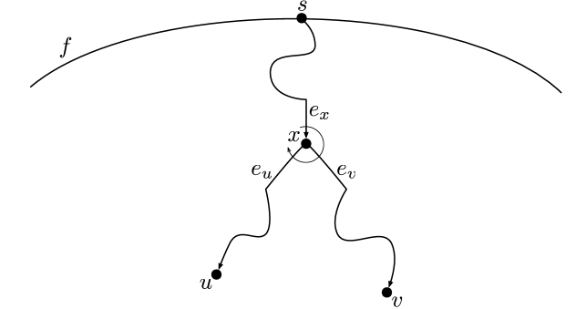
Figure 1: The clockwise order of $e_{x},e_{u},e_{v}$ around $v$ tells us whether the shortest $s$-$u$ path branches from the shortest $s$-$v$ path to the right or left.

2.4 Additively Weighted Voronoi Diagrams

Let $H$ be a weighted planar graph, $f$ a distinguished face whose vertices $S$ are called sites, and $\omega:S\to\mathbb{R}_{\geq 0}$ be a weight function on sites. We augment $H$ with large-weight edges so that it is triangulated, except for $f$. For $s\in S,v\in V(H)$, define

$$d^{\omega}(s,v)\stackrel{{\scriptstyle\operatorname{def}}}{{=}}\omega(s)+\operatorname{dist}_{H}(s,v).$$

The Voronoi diagram $\mathrm{VD}[H,S,\omega]$ is a partition of $V(H)$ into Voronoi cells, where for $s\in S$,

$$\operatorname{Vor}(s)\stackrel{{\scriptstyle\operatorname{def}}}{{=}}\{v\in V(H)\mid\forall s^{\prime}\neq s.\;(d^{\omega}(s,v),-\omega(s))<(d^{\omega}(s^{\prime},v),-\omega(s^{\prime}))\}$$

In other words, $\operatorname{Vor}(s)$ is the set of vertices that are closer to $s$ than any other site, breaking ties in favor of larger $\omega$-values. We usually work with the dual representation of a Voronoi diagram. It is constructed as follows.

• Define $\hat{S}$ to be the set of sites with nonempty Voronoi cells, i.e., $\hat{S}=\{s\in S\mid s\in\operatorname{Vor}(s)\}$. The case $|\hat{S}|=1$ is trivial, so assume $|\hat{S}|\geq 2$.

• Add large-weight dummy edges to $H$ so that $\hat{S}$ appear on the boundary of a single face $\hat{f}$, but is otherwise triangulated. Observe that this has no effect on the Voronoi cells.

• An edge is bichromatic if its endpoints are in different cells. In particular, the edges bounding $\hat{f}$ are entirely bichromatic. Define $\mathrm{VD}_{0}^{*}$ to be the (undirected) subgraph of $H^{*}$ consisting of the duals of bichromatic edges.

• Obtain $\mathrm{VD}_{1}^{*}$ from $\mathrm{VD}_{0}^{*}$ by repeatedly contracting edges incident to a degree-2 vertex, terminating when there are no degree-2 vertices, or when it becomes a self-loop. Observe that in $\mathrm{VD}_{1}^{*}$, $\hat{f}^{*}$ has degree $|\hat{S}|$ and all other vertices have degree 3; moreover, the faces of $\mathrm{VD}_{1}^{*}$ are in one-to-one correspondence with the Voronoi cells.

• We obtain $\mathrm{VD}^{*}=\mathrm{VD}^{*}[H,S,\omega]$ by splitting $\hat{f}^{*}$ into $|\hat{S}|$ degree-1 vertices, each taking an edge formerly incident to $\hat{f}^{*}$. It was proved in [20, Lemma 4.1] that $\mathrm{VD}^{*}$ is a single tree.

• We store with $\mathrm{VD}^{*}$ supplementary information useful for point location. Each degree-3 vertex $g^{*}$ in $\mathrm{VD}^{*}$ corresponds a trichromatic face $g$ whose three vertices, say $y_{0},y_{1},y_{2}$, belong to different Voronoi cells. We store in $\mathrm{VD}^{*}$ the sites $s_{0},s_{1},s_{2}\in S$ such that $y_{i}\in\operatorname{Vor}(s_{i})$. We also store a centroid decomposition of $\mathrm{VD}^{*}$. A centroid of a tree $T$ is a vertex $c$ that partitions the edge set of $T$ into disjoint subtrees $T_{1},\ldots,T_{\deg(c)}$, each containing at most $(|E(T)|+1)/2$ edges, and each containing $c$ as a leaf. The decomposition is a tree rooted at $c$, whose subtrees are the centroid decompositions of $T_{1},\ldots,T_{\deg(c)}$. The recursion bottoms out when $T$ consists of a single edge, which is represented as a single (leaf) node in the centroid decomposition.

(a)
(b)	(c)

Figure 2: (a) The original $H$ is a triangulated grid, with $f$ being the exterior face. The boundary vertices $\hat{S}$ with non-empty Voronoi cells are marked with colored halos. Edges are added so that $\hat{S}$ are on the exterior face $\hat{f}$. The vertices of $\mathrm{VD}^{*}$ are the duals of trichromatic faces, and those derived by splitting $\hat{f}^{*}$ into $|\hat{S}|$ vertices. The edges of $\mathrm{VD}^{*}$ correspond to paths of duals of bichromatic edges. (b) The dual representation $\mathrm{VD}^{*}$. (c) A centroid decomposition of $\mathrm{VD}^{*}$.

The most important query on Voronoi diagrams is point location.

Lemma 2.2.

(Gawrychowski et al. [20]) The $\boldsymbol{\mathsf{PointLocate}}(\mathrm{VD}^{*}[H,S,\omega],v)$ function is given the dual representation of a Voronoi diagram $\mathrm{VD}^{*}[H,S,\omega]$ and a vertex $v\in V(H)$ and reports the $s\in S$ for which $v\in\operatorname{Vor}(s)$. Given access to an MSSP data structure for $H$ with source-set $S$ and query time $\tau$, we can answer $\boldsymbol{\mathsf{PointLocate}}(\mathrm{VD}^{*}[H,S,\omega],v)$ queries in $O(\tau\cdot\log|H|)$ time.

The challenge in our data structure (as in [9]) is to do point location when our space budget precludes storing all the relevant MSSP structures. Nonetheless, we do make use of $\boldsymbol{\mathsf{PointLocate}}$ when the MSSP data structures are available.

3 The Distance Oracle

As in [9], the distance oracle is based on an $\vec{r}$-decomposition, $\vec{r}=(r_{m},\ldots,r_{1})$, where $r_{i}=n^{i/m}$ and $m$ is a parameter. Suppose we want to compute $\operatorname{dist}_{G}(u,v)$. Let $R_{0}=\{u\}$ be the artificial level-0 region containing $u$ and $R_{i}\in\mathcal{R}_{i}$ be the level-$i$ ancestor of $R_{0}$. (Throughout the paper, we will use “$R_{i}$” to refer specifically to the level-$i$ ancestor of $R_{0}=\{u\}$, as well as to a generic region at level-$i$. Surprisingly, this will cause no confusion.) Let $t$ be the smallest index for which $v\not\in R_{t}$ but $v\in R_{t+1}$. Define $u_{i}$ to be the last vertex on $\partial R_{i}$ encountered on the shortest path from $u$ to $v$. The main task of the distance query algorithm is to compute the sequence $(u=u_{0},\ldots,u_{t})$. Suppose that we know the identity of $u_{i}$ and $t>i$. Finding $u_{i+1}$ now amounts to a point location problem in $\mathrm{VD}^{*}[R_{i+1}^{\operatorname{out}},\partial R_{i+1},\omega]$, where $\omega(s)$ is the distance from $u_{i}$ to $s\in\partial R_{i+1}$. However, we cannot apply the fast $\boldsymbol{\mathsf{PointLocate}}$ routine because we cannot afford to store an MSSP structure for every $(R_{i+1}^{\operatorname{out}},\partial R_{i+1})$, since $|R_{i+1}^{\operatorname{out}}|=\Omega(|G|)$. Our point location routine narrows down the number of possibilities for $u_{i+1}$ to at most two candidates in $O(\kappa\log^{2+o(1)}n)$ time, then decides between them using two recursive distance queries, but starting at a higher level in the hierarchy. There are about $2^{m}$ recursive calls in total, leading to a $O(2^{m}\kappa\log^{2+o(1)}n)$ query time.

The data structure is composed of several parts. Parts (A) and (B) are explained below, while parts (C)–(E) will be revealed in Section 4.2.

1. (MSSP Structures) For each $i\in[0,m-1]$ and each region $R_{i}\in\mathcal{R}_{i}$ with parent $R_{i+1}\in\mathcal{R}_{i+1}$, we store an MSSP data structure (Lemma 2.1) for the graph $R_{i}^{\operatorname{out}}$, and source set $\partial R_{i}$. However, the structure only answers queries for $s\in\partial R_{i}$ and $u,v\in R_{i}^{\operatorname{out}}\cap R_{i+1}$. Rather than represent the full SSSP tree from each root on $s\in\partial R_{i}$, the MSSP data structure only stores the tree induced by $R_{i}^{\operatorname{out}}\cap R_{i+1}$, i.e., the parent of any vertex $v\in R_{i}^{\operatorname{out}}\cap R_{i+1}$ is its nearest ancestor $v^{\prime}$ in the SSSP tree such that $v^{\prime}\in R_{i}^{\operatorname{out}}\cap R_{i+1}$. If $(v^{\prime},v)$ is a “shortcut” edge corresponding to a path in $R_{i+1}^{\operatorname{out}}$, it has weight $\operatorname{dist}_{R_{i}^{\operatorname{out}}}(v^{\prime},v)$.

   We fix a $\kappa$ and let the update time in the dynamic tree data structure be $O(\kappa n^{1/\kappa})$ time. Thus, the space for this structure is $O((|R_{i}^{\operatorname{out}}\cap R_{i+1}|+|\partial R_{i}|\cdot|\partial R_{i+1}|)\cdot\kappa n^{1/\kappa})=O(r_{i+1}\cdot\kappa n^{1/\kappa})$ since each edge in $R_{i}^{\operatorname{out}}\cap R_{i+1}$ is swapped into and out of the SSSP tree once [28], and the number of shortcut edges on $\partial R_{i+1}$ swapped into and out of the SSSP is at most $|\partial R_{i+1}|$ for each of the $|\partial R_{i}|$ sources. Over all $i$ and $\Theta(n/r_{i})$ choices of $R_{i}$, the space is $O(m\kappa n^{1+1/m+1/\kappa})$ since $r_{i+1}/r_{i}=n^{1/m}$.

2. (Voronoi Diagrams) For each $i\in[0,m-1]$ and $R_{i}\in\mathcal{R}_{i}$ with parent $R_{i+1}\in\mathcal{R}_{i+1}$, and each $q\in\partial R_{i}$, define $\mathrm{VD}^{*}_{\operatorname{out}}(q,R_{i+1})$ to be $\mathrm{VD}^{*}[R_{i+1}^{\operatorname{out}},\partial R_{i+1},\omega]$, with $\omega(s)=\operatorname{dist}_{G}(q,s)$. The space to store the dual diagram and its centroid decomposition is $O(|\partial R_{i+1}|)=O(\sqrt{r_{i+1}})$. Over all choices for $i,R_{i},$ and $q$, the space is $O(mn^{1+1/(2m)})$ since $\sqrt{r_{i+1}/r_{i}}=n^{1/(2m)}$.

Due to our tie-breaking rule in the definition of $\operatorname{Vor}(\cdot)$, locating $u_{i+1}$ ($t\geq i+1$) is tantamount to performing a point location on a Voronoi diagram in part (B) of the data structure.

Lemma 3.1.

Suppose that $q\in\partial R_{i}$ and $v\not\in R_{i+1}$. Consider the Voronoi diagram associated with $\mathrm{VD}^{*}_{\operatorname{out}}(q,R_{i+1})$ with sites $\partial R_{i+1}$ and additive weights defined by distances from $q$ in $G$. Then $v\in\operatorname{Vor}(s)$ if and only if $s$ is the last $\partial R_{i+1}$-vertex on the shortest path from $q$ to $v$ in $G$, and $d^{\omega}(s,v)=\operatorname{dist}_{G}(q,v)$.

Proof.

By definition, $d^{\omega}(s,v)$ is the length of the shortest path from $q$ to $v$ that passes through $s$ and whose $s$-$v$ suffix does not leave $R_{i+1}^{\operatorname{out}}$. Thus, $d^{\omega}(s,v)\geq\operatorname{dist}_{G}(q,v)$ for every $s$, and $d^{\omega}(s,v)=\operatorname{dist}_{G}(q,v)$ for some $s$. Because of our assumption that all edges are strictly positive, and our tie-breaking rule for preferring larger $\omega$-values in the definition of $\operatorname{Vor}(\cdot)$, if $v\in\operatorname{Vor}(s)$ then $s$ must be the last $\partial R_{i+1}$-vertex on the shortest $q$-$v$ path. ∎

3.1 The Query Algorithm

A distance query is given $u,v\in V(G)$. We begin by identifying the level-0 region $R_{0}=\{u\}\in\mathcal{R}_{0}$ and call the function $\boldsymbol{\mathsf{Dist}}(u,v,R_{0})$. In general, the function $\boldsymbol{\mathsf{Dist}}(u_{i},v,R_{i})$ takes as arguments a region $R_{i}$, a source vertex $u_{i}$ on the boundary $\partial R_{i}$, and a target vertex $v\not\in R_{i}$. It returns a value $d$ such that

$$\operatorname{dist}_{G}(u_{i},v)\leq d\leq\operatorname{dist}_{R_{i}^{\operatorname{out}}}(u_{i},v).$$ (1)

Note that $R_{0}^{\operatorname{out}}=G$, so the initial call to this function correctly computes $\operatorname{dist}_{G}(u,v)$. When $v$ is “close” to $u_{i}$ ($v\in R_{i}^{\operatorname{out}}\cap R_{i+1}$) it computes $\operatorname{dist}_{R_{i}^{\operatorname{out}}}(u_{i},v)$ without recursion, using part (A) of the data structure. When $v\in R_{i+1}^{\operatorname{out}}$ it performs point location using the function $\boldsymbol{\mathsf{CentroidSearch}}$, which culminates in up to two recursive calls to $\boldsymbol{\mathsf{Dist}}$ on the level-$(i+1)$ region $R_{i+1}$. Thus, the correctness of $\boldsymbol{\mathsf{Dist}}$ hinges on whether $\boldsymbol{\mathsf{CentroidSearch}}$ correctly computes distances when $v\in R_{i+1}^{\operatorname{out}}$.

Algorithm 1 $\boldsymbol{\mathsf{Dist}}(u_{i},v,R_{i})$

1:A region $R_{i}$, a source $u_{i}\in\partial R_{i}$ and a destination $v\in R_{i}^{\operatorname{out}}$.

2:A value $d$ such that $\operatorname{dist}_{G}(u_{i},v)\leq d\leq\operatorname{dist}_{R_{i}^{\operatorname{out}}}(u_{i},v)$.

3:if $v\in R_{i}^{\operatorname{out}}\cap R_{i+1}$ then $\triangleright$ I.e., $i=t$

4:     return $d\leftarrow\operatorname{dist}_{R_{i}^{\operatorname{out}}}(u_{i},v)$ $\triangleright$ Part (A)

5:end if$\triangleright$ $v\in R_{i+1}^{\operatorname{out}}$

6:$f^{*}\leftarrow$ root of the centroid decomposition of $\mathrm{VD}^{*}_{\operatorname{out}}(u_{i},R_{i+1})$

7:return $d\leftarrow\boldsymbol{\mathsf{CentroidSearch}}(\mathrm{VD}^{*}_{\operatorname{out}}(u_{i},R_{i+1}),v,f^{*})$

The procedure $\boldsymbol{\mathsf{CentroidSearch}}$ is given $u_{i}\in\partial R_{i}$, $v\in R_{i+1}^{\operatorname{out}}$, $\mathrm{VD}^{*}_{\operatorname{out}}=\mathrm{VD}^{*}_{\operatorname{out}}(u_{i},R_{i+1})$ and a node $f^{*}$ on the centroid decomposition of $\mathrm{VD}^{*}_{\operatorname{out}}$. It ultimately computes $u_{i+1}\in\partial R_{i+1}$ for which $v\in\operatorname{Vor}(u_{i+1})$ and returns

$$\omega(u_{i+1})+\boldsymbol{\mathsf{Dist}}(u_{i+1},v,R_{i+1}) \boldsymbol{\mathsf{CentroidSearch}}$$ Line 5 or 9 of

$$\leq\operatorname{dist}_{G}(u_{i},u_{i+1})+\operatorname{dist}_{R_{i+1}^{\operatorname{out}}}(u_{i+1},v) \omega \boldsymbol{\mathsf{Dist}}$$ Defn. of ; guarantee of (Eqn. (1))

$$=\operatorname{dist}_{G}(u_{i},v).$$ Lemma 3.1

The algorithm is recursive, and bottoms out in one of two base cases (Line 5 or Line 9). The first way the recursion can end is if we reach the bottom of the centroid decomposition. If $f^{*}$ is a leaf of the decomposition, it corresponds to an edge in $\mathrm{VD}^{*}_{\operatorname{out}}$ separating the Voronoi cells of two sites, say $s_{1}$ and $s_{2}$. At this point we know that either $u_{i+1}=s_{1}$ or $u_{i+1}=s_{2}$, and determine which case is true with two recursive calls to $\boldsymbol{\mathsf{Dist}}(s_{j},v,R_{i+1})$, $j\in\{1,2\}$ (Lines 2–5). In general, $f^{*}$ is dual to a trichromatic face $f$ composed of three vertices $y_{0},y_{1},y_{2}$ in clockwise order, which are, respectively, in distinct Voronoi cells of $s_{0},s_{1},s_{2}$. The three shortest $s_{j}$-$y_{j}$ paths and $f$ partition the vertices of $R_{i+1}^{\operatorname{out}}$ into six parts, namely the shortest $s_{j}$-$y_{j}$ paths themselves, and the interiors of the regions bounded by $\partial R_{i+1}$, two of the $s_{j}$-$y_{j}$ paths and an edge of $f$. See Figure 3. The $\boldsymbol{\mathsf{Navigation}}$ function returns a pair $(\operatorname{flag},a^{*})$ that identifies which part $v$ is in. If $\operatorname{flag}=\operatorname{terminal}$ then $a^{*}\in\{s_{0},s_{1},s_{2}\}$ is interpreted as a site, indicating that $v$ lies on the shortest path from $a^{*}$ to its $f$-vertex. In this case we return $\omega(a^{*})+\boldsymbol{\mathsf{Dist}}(a^{*},v,R_{i+1})=\operatorname{dist}_{G}(u_{i},v)$ with just one call to $\boldsymbol{\mathsf{Dist}}$. If $\operatorname{flag}=\operatorname{nonterminal}$ then $a^{*}$ is the correct child of $f^{*}$ in the centroid decomposition. In particular, $f^{*}$ is incident to three edges $e_{0}^{*},e_{1}^{*},e_{2}^{*}$ dual to $\{y_{0},y_{2}\},\{y_{1},y_{0}\},\{y_{2},y_{1}\}$. The children of $f^{*}$ in the centroid decomposition are $f_{0}^{*},f_{1}^{*},f_{2}^{*}$, with $f_{j}^{*}$ ancestral to $e_{j}^{*}$. We have $a^{*}=f_{j}^{*}$ if $v$ lies to the right of the chord $(s_{j},\ldots,y_{j},y_{j-1},\ldots,s_{j-1})$ in $R_{i+1}^{\operatorname{out}}$. For example, in Figure 3, $v$ lies to the right of the $(s_{0},\ldots,y_{0},y_{2},\ldots,s_{2})$ path. In this case we continue the search recursively from $a^{*}=f_{0}^{*}$.

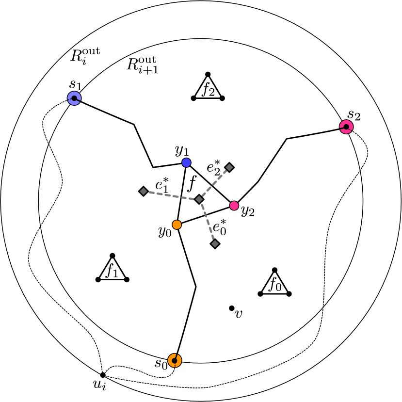
Figure 3: Here $f^{*}$ is a degree-3 vertex in $\mathrm{VD}^{*}_{\operatorname{out}}(u_{i},R_{i+1})$, corresponding to a trichromatic face $f$ on vertices $y_{0},y_{1},y_{2}$, which are in the Voronoi cells of $s_{0},s_{1},s_{2}$ on the boundary $\partial R_{i+1}^{\operatorname{out}}$. The shortest $s_{j}$-$y_{j}$ paths partition $V(R_{i+1}^{\operatorname{out}})$ into six parts: the three shortest paths and the three regions bounded by them and $f$. Let $e_{0}^{*},e_{1}^{*},e_{2}^{*}$ be the edges in $\mathrm{VD}^{*}_{\operatorname{out}}$ dual to $\{y_{0},y_{2}\},\{y_{1},y_{0}\},\{y_{2},y_{1}\}$. In the centroid decomposition $e_{0}^{*},e_{1}^{*},e_{2}^{*}$ are in separate subtrees of $f^{*}$. Let $f_{j}^{*}$ be the child of $f^{*}$ ancestral to $e_{j}^{*}$, which is either $e_{j}^{*}$ itself, or a trichromatic face to the right of the “chord” $(s_{j},\ldots,y_{j},y_{j-1},\ldots,s_{j-1})$. $\boldsymbol{\mathsf{CentroidSearch}}$ locates the site whose Voronoi cell contains $v$ via recursion. It calls $\boldsymbol{\mathsf{Navigation}}$, a function that finds which of the 6 parts contains $v$. If $v$ lies on an $s_{j}$-$y_{j}$ path the $\boldsymbol{\mathsf{CentroidSearch}}$ recursion terminates; otherwise it recurses on the correct child $f_{j}^{*}$ of $f^{*}$.

Algorithm 2 $\boldsymbol{\mathsf{CentroidSearch}}(\mathrm{VD}^{*}_{\operatorname{out}}(u_{i},R_{i+1}),v,f^{*})$

1:The dual representation $\mathrm{VD}^{*}_{\operatorname{out}}=\mathrm{VD}^{*}_{\operatorname{out}}(u_{i},R_{i+1})$ of a Voronoi diagram with additive weights $\omega(s)=\operatorname{dist}_{G}(u_{i},s)$, a vertex $v\in R_{i+1}^{\operatorname{out}}$, and a node $f^{*}$ in the centroid decomposition of $\mathrm{VD}^{*}_{\operatorname{out}}$.

2:The distance $\operatorname{dist}_{G}(u_{i},v)$.

3:if $f^{*}$ is a leaf in the centroid decomposition (an edge in $\mathrm{VD}^{*}_{\operatorname{out}}$) then

4:     $s_{1},s_{2}\leftarrow$ sites whose Voronoi cells are bounded by $f^{*}$ $\triangleright$ Candidates for $u_{i+1}$

5:     $d_{1}\leftarrow\omega(s_{1})+\boldsymbol{\mathsf{Dist}}(s_{1},v,R_{i+1})$

6:     $d_{2}\leftarrow\omega(s_{2})+\boldsymbol{\mathsf{Dist}}(s_{2},v,R_{i+1})$

7:     return $\min(d_{1},d_{2})$

8:end if

9:$(\operatorname{flag},a^{*})\leftarrow\boldsymbol{\mathsf{Navigation}}(\mathrm{VD}^{*}_{\operatorname{out}}(u_{i},R_{i+1}),v,f^{*})$

10:if $\operatorname{flag}=\operatorname{terminal}$ then $\triangleright$ $a^{*}$ is interpreted as a site

11:     return $\omega(a^{*})+\boldsymbol{\mathsf{Dist}}(a^{*},v,R_{i+1})$ $\triangleright$ $a^{*}=u_{i+1}$

12:else  (i.e., $\operatorname{flag}=\operatorname{nonterminal}$) $\triangleright$ $a^{*}$ is the centroid child of $f^{*}$

13:     return $\boldsymbol{\mathsf{CentroidSearch}}(\mathrm{VD}^{*}_{\operatorname{out}}(u_{i},R_{i+1}),v,a^{*})$

14:end if

Lemma 3.2.

$\boldsymbol{\mathsf{CentroidSearch}}$ correctly computes $\operatorname{dist}_{G}(u_{i},v)$

Proof.

Define $f,y_{j},s_{j},e_{j}^{*},f_{j}^{*}$ as usual, and let $u_{i+1}$ be such that $v\in\operatorname{Vor}(u_{i+1})$. The loop invariant is that in the subtree of the centroid decomposition rooted at $f^{*}$, there is some leaf edge on the boundary of the cell $\operatorname{Vor}(u_{i+1})$. This is clearly true in the intial recursive call, when $f^{*}$ is the root of the centroid decomposition. Suppose that $\boldsymbol{\mathsf{Navigation}}$ tells us that $v$ lies to the right of the oriented chord $C^{\star}=(s_{j},\ldots,y_{j},y_{j-1},\ldots,s_{j-1})$. Observe that since the $s_{j}$-$y_{j}$ and $s_{j-1}$-$y_{j-1}$ shortest paths are monochromatic, all edges of the centroid decomposition correspond to paths in $G^{*}$ that lie strictly to the left or right of $C^{\star}$, with the exception of $e_{j}^{*}$. Moreover, since $v\in\operatorname{Vor}(u_{i+1})$, $\operatorname{Vor}(u_{i+1})$ must be bounded by some edge that is either $e_{j}^{*}$ or one entirely to the right of $C^{\star}$, from which it follows that $f_{j}^{*}=a^{*}$ is ancestral to at least one edge bounding $\operatorname{Vor}(u_{i+1})$. When $f^{*}$ is a single edge on the boundary of $\operatorname{Vor}(s_{1}),\operatorname{Vor}(s_{2})$ the loop invariant guarantees that either $u_{i+1}=s_{1}$ or $u_{i+1}=s_{2}$; suppose that $u_{i+1}=s_{1}$. It follows from the specification of $\boldsymbol{\mathsf{Dist}}$ (Eqn. (1)) and Lemma 3.1 that

$$d_{1}=\omega(s_{1})+\boldsymbol{\mathsf{Dist}}(s_{1},v,R_{i+1})\leq\operatorname{dist}_{G}(u_{i},s_{1})+\operatorname{dist}_{R_{i+1}^{\operatorname{out}}}(s_{1},v)=\operatorname{dist}_{G}(u_{i},v).$$

Furthermore,

$$d_{2}=\omega(s_{2})+\boldsymbol{\mathsf{Dist}}(s_{2},v,R_{i+1})\geq\operatorname{dist}_{G}(u_{i},s_{2})+\operatorname{dist}_{G}(s_{2},v)\geq\operatorname{dist}_{G}(u_{i},v),$$

so in this base case $\boldsymbol{\mathsf{CentroidSearch}}$ correctly returns $d_{1}=\operatorname{dist}_{G}(u_{i},v)$. If $\boldsymbol{\mathsf{Navigation}}$ ever reports that $v$ is on an $s_{j}$-$y_{j}$ path, then by definition $v\in\operatorname{Vor}(s_{j})$. By the specification of $\boldsymbol{\mathsf{Dist}}$ (Eqn. (1)) and Lemma 3.1 we have

$$\omega(s_{j})+\boldsymbol{\mathsf{Dist}}(s_{j},v,R_{i+1})\leq\operatorname{dist}_{G}(u_{i},s_{j})+\operatorname{dist}_{R_{i+1}^{\operatorname{out}}}(s_{j},v)=\operatorname{dist}_{G}(u_{i},v)$$

and the base case on Lines 8–9 also works correctly. ∎

Thus, the main challenge is to design an efficient $\boldsymbol{\mathsf{Navigation}}$ function, i.e., to solve the restricted point location problem in $R_{i+1}^{\operatorname{out}}$ depicted in Figure 3. Whereas Charalampopoulos et al. [9] solve this problem using several more recursive calls to $\boldsymbol{\mathsf{Dist}}$, we give a new method to do this point location directly, in $O(\kappa\log^{1+o(1)}n)$ time per call to $\boldsymbol{\mathsf{Navigation}}$.

4 The Navigation Oracle

The input to $\boldsymbol{\mathsf{Navigation}}$ is the same as $\boldsymbol{\mathsf{CentroidSearch}}$, except that $f^{*}$ is guaranteed to correspond to a trichromatic face $f$. Define $y_{j},s_{j},e_{j},f_{j}$, $j\in\{0,1,2\}$ as in the discussion of $\boldsymbol{\mathsf{CentroidSearch}}$. The $\boldsymbol{\mathsf{Navigation}}$ function determines the location of $v$ relative to $f$ and the shortest $s_{j}$-$y_{j}$ paths. It delegates nearly all the actual computation to two functions: $\boldsymbol{\mathsf{SitePathIndicator}}$, which returns a boolean indicating whether $v$ is on the shortest $s_{j}$-$y_{j}$ path, and $\boldsymbol{\mathsf{ChordIndicator}}$, which indicates whether $v$ lies strictly to the right of the oriented chord $(s_{j},\ldots,y_{j},y_{j-1},\dots,s_{j-1})$. If so, we return the centroid child $f_{j}^{*}$ of $f^{*}$ in this region. Three calls each to $\boldsymbol{\mathsf{SitePathIndicator}}$ and $\boldsymbol{\mathsf{ChordIndicator}}$ suffice to determine the location of $v$.

Algorithm 3 $\boldsymbol{\mathsf{Navigation}}(\mathrm{VD}^{*}_{\operatorname{out}}(u_{i},R_{i+1}),v,f^{*})$

1:The dual representation $\mathrm{VD}^{*}_{\operatorname{out}}(u_{i},R_{i+1})$ of a Voronoi diagram, a vertex $v\in R_{i+1}^{\operatorname{out}}$, and a centroid $f^{*}$ in the centroid decomposition. The face $f$ is on $y_{0},y_{1},y_{2}$, which are in the Voronoi cells of $s_{0},s_{1},s_{2}$, and $f_{j}^{*}$ is the child of $f^{*}$ containing the edge dual to $\{y_{j},y_{j-1}\}$.

2:$(\operatorname{terminal},s_{j})$ if $v$ is on the shortest $s_{j}$-$y_{j}$ path, or $(\operatorname{nonterminal},f_{j}^{*})$ where $f_{j}^{*}$ is the child of $f^{*}$ ancestral to an edge bounding $v$’s Voronoi cell.

3:$s_{0},s_{1},s_{2}\leftarrow$ sites corresponding to $f^{*}$

4:for $j=0,1,2$ do

5:     if $\boldsymbol{\mathsf{SitePathIndicator}}(\mathrm{VD}^{*}_{\operatorname{out}}(u_{i},R_{i+1}),v,f^{*},j)$ returns True then

6:         return $(\operatorname{terminal},s_{j})$

7:     end if

8:end for

9:for $j=0,1,2$ do

10:     if $\boldsymbol{\mathsf{ChordIndicator}}(\mathrm{VD}^{*}_{\operatorname{out}}(u_{i},R_{i+1}),v,f^{*},j)$ returns True then

11:         return $(\operatorname{nonterminal},f_{j}^{*})$

12:     end if

13:end for

In Section 4.1 we formally introduce the notion of chords used informally above, as well as some related concepts like laminar sets of chords and maximal chords. In Section 4.2 we introduce parts (C)-(E) of the data structure used to support $\boldsymbol{\mathsf{Navigation}}$. The functions $\boldsymbol{\mathsf{SitePathIndicator}}$ and $\boldsymbol{\mathsf{ChordIndicator}}$ are presented in Sections 4.3 and 4.4.

4.1 Chords and Pieces

We begin by defining the key concepts of our point location method: chords, laminar chord sets, pieces, and the occludes relation.

Definition 4.1.

(Chords) Fix an $R$ in the $\vec{r}$-decomposition and two vertices $c_{0},c_{1}\in\partial R$. An oriented simple path $\overrightarrow{c_{0}c_{1}}$ is a chord of $R^{\operatorname{out}}$ if it is contained in $R^{\operatorname{out}}$ and is internally vertex-disjoint from $\partial R$. When the orientation is irrelevant we write it as $\overline{c_{0}c_{1}}$.

Definition 4.2.

(Laminar Chord Sets) A set of chords $\mathcal{C}$ for $R^{\operatorname{out}}$ is laminar (non-crossing) if for any two such chords $C=\overrightarrow{c_{0}c_{1}},C^{\prime}=\overrightarrow{c_{2}c_{3}}$, if there exists a $v\in(C\cap C^{\prime})-\partial R$ then the subpaths from $c_{0}$ to $v$ and from $c_{2}$ to $v$ are identical; in particular $c_{0}=c_{2}$.

The orientation of chords does not always coincide with a natural orientation of paths defined by the algorithm. For example, in Figure 3, the oriented chord $\overrightarrow{s_{0}s_{2}}=(s_{0},\ldots,y_{0},y_{2},\ldots,s_{2})$ is composed of three parts: a shortest $s_{0}$-$y_{0}$ path (whose natural orientation coincides with that of $\overrightarrow{s_{0}s_{2}}$), the edge $\{y_{0},y_{2}\}$ (which has no natural orientation in this context), and the shortest $s_{2}$-$y_{2}$ path (whose natural orientation is the reverse of its orientation in $\overrightarrow{s_{0}s_{2}}$). The orientation serves two purposes. In Definition 4.1 we can speak unambiguously about the parts of $R^{\operatorname{out}}$ to the right and left of $\overrightarrow{s_{0}s_{2}}$. In Definition 4.2 the role of the orientation is to ensure that the partition of $R^{\operatorname{out}}$ into pieces induced by $\mathcal{C}$ can be represented by a tree, as we show in Lemma 4.1.

Definition 4.3.

(Pieces) A laminar chord set $\mathcal{C}$ for $R^{\operatorname{out}}$ partitions the faces of $R^{\operatorname{out}}$ into pieces, excluding the face on $\partial R$. Two faces $f,g$ are in the same piece iff $f^{*}$ and $g^{*}$ are connected by a path in $(R^{\operatorname{out}})^{*}$ that avoids to duals of edges in $\mathcal{C}$ and edges along the boundary cycle on $\partial R$. A piece is regarded as the subgraph induced by its faces, i.e., it includes their constituent vertices and edges. Two pieces $P_{1},P_{2}$ are adjacent if there is an edge $e$ on the boundary of $P_{1}$ and $P_{2}$ and $e$ is in a unique chord of $\mathcal{C}$. See Figure 4.

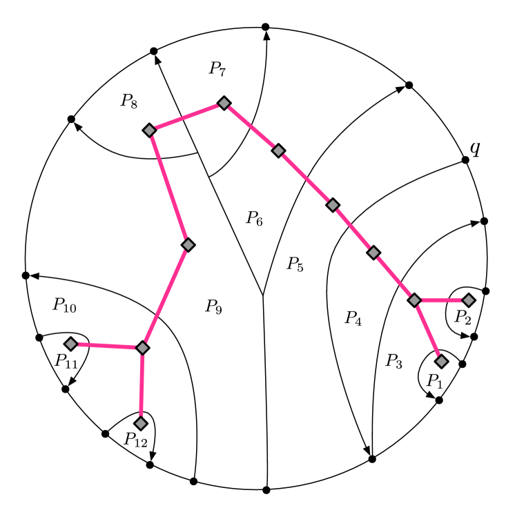
Figure 4: A laminar set of chords partition $R^{\operatorname{out}}$ into pieces. Observe that the chords separating pieces $P_{5}$–$P_{9}$ overlap in certain prefixes. The piece tree is indicated by diamond verties and pink edges. Note two pieces (e.g. $P_{5}$ and $P_{9}$) may share a boundary, but not be adjacent.

Lemma 4.1.

Suppose $\mathcal{C}$ is a laminar chord set for $R^{\operatorname{out}}$, $\mathcal{P}=\mathcal{P}(\mathcal{C})$ is the corresponding piece set and $\mathcal{E}$ are pairs of adjacent pieces. Then $\mathcal{T}=(\mathcal{P},\mathcal{E})$ is a tree, called the piece tree induced by $\mathcal{C}$.

Proof.

The claim is clearly true when $\mathcal{C}$ contains zero or one chords, so we will try to reduce the general case to this case via a peeling argument. We will find a piece $P$ with degree 1 in $\mathcal{T}$, remove it and the chord bounding it, and conclude by induction that the truncated instance is a tree. Reattaching $P$ implies $\mathcal{T}$ is a tree.

Let $C=\overrightarrow{c_{0}c_{1}}\in\mathcal{C}$ be a chord such that no edge of any other chord appears strictly to one side of $C$, say to the right of $C$. Let $P$ be the piece to the right of $C$. (In Figure 4 the chords bounding $P_{1},P_{2},P_{11},P_{12}$ would be eligible to be $C$.) Let $C=(c_{0}=v_{0},v_{1},v_{2},\ldots,v_{k}=c_{1})$ and $v_{j^{\star}}$ be such that the edges of the suffix $(v_{j^{\star}},\ldots,v_{k})$ are on no other chord, meaning the vertices $\{v_{j^{\star}+1},\ldots,v_{k-1}\}$ are on no other chord. Let $g_{j}$ be the face to the left of $(v_{j},v_{j+1})$. It follows that there is a path from $g_{j^{\star}}^{*}$ to $g_{k-1}^{*}$ in $(R^{\operatorname{out}})^{*}$ that avoids the duals of all edges in $\mathcal{C}$ and along $\partial R$. All pieces adjacent to $P$ contain some face among $\{g_{j^{\star}},\ldots,g_{k-1}\}$, but these are in a single piece, hence $P$ corresponds to a degree-1 vertex in $\mathcal{T}$. Let $P$ be bounded by $C$ and an interval $B$ of the boundary cycle on $\partial R$. Obtain the “new” $R^{\operatorname{out}}$ by cutting along $C$ and removing $P$, the new $\partial R$ by substituting $C$ for $B$, and the new chord-set $\mathcal{C}$ by removing $C$ and trimming any chords that shared a non-empty prefix with $C$. By induction the resulting piece-adjacency graph is a tree; reattaching $P$ as a degree-1 vertex shows $\mathcal{T}$ is a tree. ∎

Definition 4.4.

(Occludes Relation) Fix $R^{\operatorname{out}}$, chord $C$, and two faces $f,g$, neither of which is the hole defined by $\partial R$. If $f$ and $g$ are on opposite sides of $C$, we say that from vantage $f$, $C$ occludes $g$. Let $\mathcal{C}$ be a set of chords. We say $C\in\mathcal{C}$ is maximal in $\mathcal{C}$ with respect to a vantage $f$ if there is no $C^{\prime}\in\mathcal{C}$ such that $C^{\prime}$ occludes a strict superset of the faces that $C$ occludes. (Note that the orientation of chords is irrelevant to the occludes relation.)

It follows from Definition 4.4 that if $\mathcal{C}$ is laminar, the set of maximal chords with respect to $f$ are exactly those chords intersecting the boundary of $f$’s piece in $\mathcal{P}(\mathcal{C})$.

We can also speak unambiguously about a chord $C$ occluding a vertex or edge not on $C$, from a certain vantage. Specifically, we can say that from some vantage, $C$ occludes an interval of the boundary cycle on $\partial R$, say according to a clockwise traversal around the hole on $\partial R$ in $R^{\operatorname{out}}$. This will be used in the $\boldsymbol{\mathsf{ChordIndicator}}$ procedure of Section 4.4.2.

4.2 Data Structures for Navigation

Parts (C)–(E) of the data structure are used to implement the $\boldsymbol{\mathsf{SitePathIndicator}}$ and $\boldsymbol{\mathsf{ChordIndicator}}$ functions.

1. (More Voronoi Diagrams) For each $i$, each $R_{i}\in\mathcal{R}_{i}$, and each $q\in\partial R_{i}$, we store $\mathrm{VD}^{*}_{\operatorname{out}}(q,R_{i})$, which is $\mathrm{VD}^{*}[R_{i}^{\operatorname{out}},\partial R_{i},\omega]$, where $\omega(s)=\operatorname{dist}_{G}(q,s)$. The total space for these diagrams is $\tilde{O}(n)$ and dominated by part (B).

2. (Chord Trees; Piece Trees) For each $i$, each $R_{i}\in\mathcal{R}_{i}$, and source $q\in\partial R_{i}$, we store the SSSP tree from $q$ induced by $\partial R_{i}$ as a chord tree $T_{q}^{R_{i}}$. In particular, the parent of $x\in\partial R_{i}$ in $T_{q}^{R_{i}}$ is the nearest ancestor in the SSSP tree from $q$ that lies on $\partial R_{i}$. Every edge of $T_{q}^{R_{i}}$ is designated a chord if the corresponding path is contained in $R_{i}^{\operatorname{out}}$ but not in $R_{i}$, or a non-chord otherwise. Define $\mathcal{C}_{q}^{R_{i}}$ to be the set of all chords in $T_{q}^{R_{i}}$, oriented away from $q$; this is clearly a laminar set since shortest paths are unique and all prefixes of shortest paths are shortest paths. Define $\mathcal{P}_{q}^{R_{i}}$ to be the corresponding partition of $R_{i}^{\operatorname{out}}$ into pieces, and $\mathcal{T}_{q}^{R_{i}}$ the corresponding piece tree. Define $T_{q}^{R_{i}}[x]$ to be the path from $q$ to $x$ in $T_{q}^{R_{i}}$, $\mathcal{C}_{q}^{R_{i}}[x]$ the corresponding chord-set, and $\mathcal{P}_{q}^{R_{i}}[x]$ the corresponding piece-set.

   The data structure answers the following queries

   $\boldsymbol{\mathsf{MaximalChord}}(R_{i},q,x,P,P^{\prime})$:

   We are given $R_{i}$, $q,x\in\partial R_{i}$, a piece $P\in\mathcal{P}_{q}^{R_{i}}$, and possibly another piece $P^{\prime}\in\mathcal{P}_{q}^{R_{i}}$ (which may be Null). If $P^{\prime}$ is Null, return any maximal chord in $\mathcal{C}_{q}^{R_{i}}[x]$ from vantage $P$. If $P^{\prime}$ is not Null, return the maximal chord $\mathcal{C}_{q}^{R_{i}}[x]$ (if any) that occludes $P^{\prime}$ from vantage $P$.

   $\boldsymbol{\mathsf{AdjacentPiece}}(R_{i},q,e)$:

   Here $e$ is an edge on the boundary cycle on $\partial R_{i}$. Return the unique piece in $\mathcal{P}_{q}^{R_{i}}$ with $e$ on its boundary.

3. (Site Tables; Side Tables) Fix an $i$ and a diagram $\mathrm{VD}^{*}_{\operatorname{out}}=\mathrm{VD}^{*}_{\operatorname{out}}(u^{\prime},R_{i})$ from part (B) or (C). Let $f^{*}$ be any node in the centroid decomposition of $\mathrm{VD}^{*}_{\operatorname{out}}$, with $y_{j},s_{j}$, $j\in\{0,1,2\}$ defined as usual, and let $R_{i^{\prime}}\in\mathcal{R}_{i^{\prime}}$ be the ancestor of $R_{i}$, $i^{\prime}\geq i$. Fix $j\in\{0,1,2\}$ and $i^{\prime}>i$. Define $q$ and $x$ to be the first and last vertices on the shortest $s_{j}$-$y_{j}$ path that lie on $\partial R_{i^{\prime}}$. We store $(q,x)$ and $\operatorname{dist}_{G}(u^{\prime},x)$.

   We also store whether $R_{i^{\prime}}^{\operatorname{out}}$ lies to the left or right of the site-centroid-site chord $\overrightarrow{s_{j}y_{j}y_{j-1}s_{j-1}}$ in $R_{i}^{\operatorname{out}}$, or Null if the relationship cannot be determined, i.e., if the chord crosses $\partial R_{i^{\prime}}$. These tables increase the space of (B) and (C) by a negligible $O(m)$ factor.

Part (D) of the data structure is the only one that is non-trivial to store compactly. Our strategy is as follows. We fix $R_{i}$ and $q\in\partial R_{i}$ and build a dynamic data structure for these operations relative to a dynamic subset $\hat{\mathcal{C}}\subseteq\mathcal{C}_{q}^{R_{i}}$ subject to the insertion and deletion of chords in $O(\log|\partial R_{i}|)$ time. By inserting/deleting $O(|\partial R_{i}|)$ chords in the correct order, we can arrange that $\hat{\mathcal{C}}=\mathcal{C}_{q}^{R_{i}}[x]$ at some point in time, for every $x\in\partial R_{i}$. Using the generic persistence technique for RAM data structures (see [12]) we can answer $\boldsymbol{\mathsf{MaximalChord}}$ queries relative to $\mathcal{C}_{q}^{R_{i}}[x]$ in $O(\log|\partial R_{i}|\log\log|\partial R_{i}|)$ time.

Lemma 4.2.

Part (D) of the data structure can be stored in $O(mn\log n)$ total space and answer $\boldsymbol{\mathsf{MaximalChord}}$ queries in $O(\log n\log\log n)$ time and $\boldsymbol{\mathsf{AdjacentPiece}}$ queries in $O(1)$ time.

Proof.

We first address $\boldsymbol{\mathsf{MaximalChord}}$. Let $\mathcal{T}=\mathcal{T}_{q}^{R_{i}}$ be the piece tree. The edges of $\mathcal{T}$ are in 1-1 correspondence with the chords of $\mathcal{C}=\mathcal{C}_{q}^{R_{i}}$ and if $P,P^{\prime}\in\mathcal{P}=\mathcal{P}_{q}^{R_{i}}$ are two pieces, the path from $P$ to $P^{\prime}$ in $\mathcal{T}$ crosses exactly those chords that occlude $P^{\prime}$ from vantage $P$ (and vice versa). We will argue that to implement $\boldsymbol{\mathsf{MaximalChord}}$ it suffices to design an efficient dynamic data structure for the following problem; initially all edges are unmarked.

Mark$(e)$

Mark an edge $e\in E(\mathcal{T})$.

Unmark$(e)$

Unmark $e$.

LastMarked$(P^{\prime},P)$

Return the last marked edge on the path from $P^{\prime}$ to $P$, or Null if all are unmarked.

By doing a depth-first traversal of the chord tree $T_{q}^{R_{i}}$, marking/unmarking chords as they are encountered, the set $\{e\in E(\mathcal{T})\mid e\mbox{ is marked}\}$ will be equal to $\mathcal{C}_{q}^{R_{i}}[x]$ precisely when $x$ is first encountered in DFS. To answer a $\boldsymbol{\mathsf{MaximalChord}}(R_{i},q,x,P,P^{\prime})$ query we interact with the state of the data structure when the marked set is $\mathcal{C}_{q}^{R_{i}}[x]$. If $P^{\prime}$ is not null we return LastMarked$(P^{\prime},P)$. Otherwise we pick an arbitrary (marked) chord $C\in\mathcal{C}_{q}^{R_{i}}[x]$, get the adjacent pieces $P_{1}^{\prime},P_{2}^{\prime}$ on either side of $C$, then query LastMarked$(P_{1}^{\prime},P)$ and LastMarked$(P_{2}^{\prime},P)$. At least one of these queries will return a chord and that chord is maximal w.r.t. vantage $P$. (Note that $C$ must separate $P$ from either $P_{1}^{\prime}$ or $P_{2}^{\prime}$.)

We now argue how all three operations can be implemented in $O(\log n)$ worst case time. The ideas are standard, so we do not go into great detail. Root $\mathcal{T}$ arbitrarily and subdivide every edge; the resulting tree is also called $\mathcal{T}$. Every node in $\mathcal{T}$ knows its depth. The vertices corresponding to subdivided edges may carry marks. In order to answer LastMarked queries it suffices to be able to find least common ancestors, and, given nodes $P_{d},P_{a}$, where $P_{a}$ is an ancestor of $P_{d}$, to find the first and last marked node on the path from $P_{d}$ to $P_{a}$. Decompose the vertices of $\mathcal{T}$ using a heavy path decomposition. Each vertex points to the path that it is in. Each path in the decomposition is a data structure that maintains an ordered set of its marked nodes, a pointer to the most ancestral marked node in the path, and a pointer to the parent, in $\mathcal{T}$, of the root of the path. It is straightforward to find LCAs in this structure in $O(\log n)$ time. Suppose we want the first and last marked node on the path from $P_{d}$ to $P_{a}$, an ancestor of $P_{d}$. Let $Z_{0},Z_{1},...,Z_{\ell}$, $\ell=O(\log n)$ be the heavy paths ancestral to $P_{d}$ such that $P_{d}\in Z_{0},P_{a}\in Z_{\ell}$. Let $v_{j}\in Z_{j}$ be the nearest ancestor to $P_{d}$. We can find $j^{\star}$ such that $Z_{j^{\star}}$ contains the first marked node on the $P_{d}$-$P_{a}$ path in $\ell=O(\log n)$ time by comparing $v_{j}$ against the most ancestral marked node in $Z_{j}$, $j=0,1,\ldots$. We can then find the first marked node by finding the marked predecessor of $v_{j^{\star}}$ in $Z_{j^{\star}}$, in $O(\log n)$ time. Finding the last marked node on the path from $P_{d}$ to $P_{a}$ is similar. Mark and Unmark are implemented by keeping a balanced binary search tree over the marked nodes in each heavy path.

For fixed $R_{i},q\in\partial R_{i}$ there are $O(|\partial R_{i}|)$ Mark and Unmark operations, each taking $O(\log n)$ time. Over all choices of $i,R_{i}$, and $q$ the total update time is $O(mn\log n)$. After applying generic persistence for RAM data structures (see [12]) the space becomes $O(mn\log n)$ and the query time for LastMarked becomes $O(\log n\log\log n)$.

Turning to $\boldsymbol{\mathsf{AdjacentPiece}}(R_{i},q,e)$, there are $|\partial R_{i}|^{2}$ choices of $(q,e)$. Hence all answers can be precomputed in a lookup table in $O(mn)$ space.

∎

4.3 The $\boldsymbol{\mathsf{SitePathIndicator}}$ Function

The $\boldsymbol{\mathsf{SitePathIndicator}}$ function is relatively simple. We are given $\mathrm{VD}^{*}_{\operatorname{out}}(u_{i},R_{i+1})$, $v\in R_{i+1}^{\operatorname{out}}$, a centroid $f^{*}\in R_{i+1}^{\operatorname{out}}$, $f$ being a trichromatic face on $y_{0},y_{1},y_{2}$, which are, respectively, in the Voronoi cells of $s_{0},s_{1},s_{2}\in\partial R_{i+1}$, and an index $j\in\{0,1,2\}$. We would like to know if $v$ is on the shortest $s_{j}$-to-$y_{j}$ path. Recall that $t$ is such that $v\not\in R_{t}$ but $v\in R_{t+1}$.

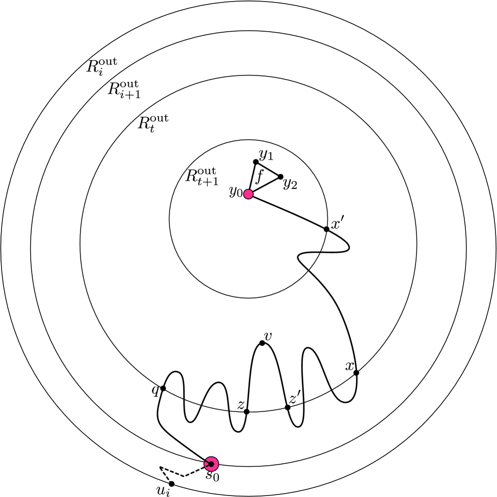
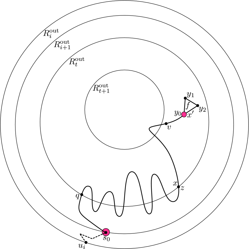
(a)	(b)

Figure 5: (a) If $z=x$ and $y_{j}$ is not in $R_{t+1}$, $x^{\prime}$ is the last boundary vertex of $\partial R_{t+1}$ on the $s_{j}$-$y_{j}$ path. (b) If $z=x$ and $y_{j}$ is in $R_{t}^{\operatorname{out}}\cap R_{t+1}$ then $x^{\prime}=y_{j}$. (Not depicted: if $y_{j}\in R_{t}$ then $x^{\prime}=x$.) We test whether $v$ is on the shortest $x$-$x^{\prime}$ path. If $z\neq x$ then $z^{\prime}$ is well defined and the position of $y_{j}$ is immaterial; we test whether $v$ is on the shortest $z$-$z^{\prime}$ path (depicted in (a)).

Using the lookup tables in part (E) of the data structure, we find the first and last vertices ($q$ and $x$) of $\partial R_{t}$ on the $s_{j}$-$y_{j}$ path. If $q,x$ do not exist then $v$ is certainly not on the $s_{j}$-$y_{j}$ path (Line 4). Using parts (A,C,E) of the data structure, we invoke $\boldsymbol{\mathsf{PointLocate}}$ to find the last point $z$ of $\partial R_{t}$ on the shortest path (in $G$) from $q$ to $v$. (See Lemma 3.1.) If $z$ is not on the path from $q$ to $x$ in $G$ (which corresponds to it not being on the path from $q$ to $x$ in $T_{q}^{R_{t}}$, stored in Part (D)), then once again $v$ is certainly not on the $s_{j}$-$y_{j}$ path (Line 8). So we may assume $z$ lies on the $q$-$x$ path. If $z=x$ then there are three cases to consider, depending on whether the destination $y_{j}$ of the path is in $R_{t}^{\operatorname{out}}\cap R_{t+1}$, or in $R_{t+1}^{\operatorname{out}}$, or in $R_{t}$. If $y_{j}\in R_{t}^{\operatorname{out}}\cap R_{t+1}$ we let $x^{\prime}=y_{j}$; if $y_{j}\in R_{t+1}^{\operatorname{out}}$ we let $x^{\prime}$ be the last vertex of $\partial R_{t+1}$ encountered on the shortest $s_{j}$-$y_{j}$ path (part (E)); and if $y_{j}\in R_{t}$ we let $x^{\prime}=x$. In all cases, $x^{\prime}$ is the last vertex of the shortest $s_{j}$-$y_{j}$ path that is contained in relevant subgraph $R_{t}^{\operatorname{out}}\cap R_{t+1}$. (Figure 5(a,b) illustrates the first two possibilities for $x^{\prime}$.) Now $v$ is on the $s_{j}$-$y_{j}$ path iff it is on the $x$-$x^{\prime}$ shortest path, which can be answered using part (A) of the data structure (Lines 19, 21). (Figure 5(b) illustrates one way for $v$ to appear on the $x$-$x^{\prime}$ path.) In the remaining case $z$ is on the shortest $q$-$x$ path but is not $x$, meaning the child $z^{\prime}$ of $z$ on $T_{q}^{R_{t}}[x]$ is well defined. If $\overrightarrow{zz^{\prime}}$ is a chord (corresponding to a path in $R_{t}^{\operatorname{out}}$) then $v$ is on the shortest $s_{j}$-$y_{j}$ path iff it is on the shortest $z$-$z^{\prime}$ path in $R_{t}^{\operatorname{out}}$, which, once again, can be answered with part (A) of the data structure (Lines 26, 28). See Figure 5(a) for an illustration of this case.

Remark 1.

Strictly speaking we cannot apply Lemma 2.2 (Gawrychowski et al. [20]) since we do not have an MSSP structure for all of $R_{t}^{\operatorname{out}}$. Part (A) only handles distance/LCA queries when the query vertices are in $R_{t}^{\operatorname{out}}\cap R_{t+1}$. It is easy to make Gawrychowski et al.’s algorithm work using parts (A) and (E) of the data structure. See the discussion at the end of Section 4.4.3.

Algorithm 4 $\boldsymbol{\mathsf{SitePathIndicator}}(\mathrm{VD}^{*}_{\operatorname{out}}(u_{i},R_{i+1}),v,f^{*},j)$

1:The dual representation $\mathrm{VD}^{*}_{\operatorname{out}}(u_{i},R_{i+1})$ of a Voronoi diagram, a vertex $v\in R_{i+1}^{\operatorname{out}}$, and an $s_{j}$-to-$y_{j}$ site-centroid shortest path ($s_{j},y_{j}$ are with respect to $f^{*}$) in $\mathrm{VD}^{*}$.

2:True if $v$ is on $s_{j}$-to-$y_{j}$ shortest path, or False otherwise.

3:$R_{t}\leftarrow$ the ancestor of $R_{i}$ s.t. $v\notin R_{t},v\in R_{t+1}$.

4:$(q,x)\leftarrow$ first and last $\partial R_{t}$ vertices on the shortest $s_{j}$-$y_{j}$ path. $\triangleright$ Part (E) of the data structure

5:if $q,x$ are Null then

6:     return False

7:end if

8:$z\leftarrow\boldsymbol{\mathsf{PointLocate}}(\mathrm{VD}^{*}_{\operatorname{out}}(q,R_{t}),v)$ $\triangleright$ Uses parts (A,C,E) of the data structure

9:if $z$ is not on $T_{q}^{R_{t}}[x]$ then

10:     return False

11:end if

12:if $z=x$ then

13:     if $y_{j}$ is in $R_{t}^{\operatorname{out}}\cap R_{t+1}$ then

14:         $x^{\prime}\leftarrow y_{j}$

15:     else if $y_{j}\not\in R_{t+1}$ then

16:         $x^{\prime}\leftarrow$ last $\partial R_{t+1}$ vertex on $s_{j}$-$y_{j}$ path. $\triangleright$ Part (E)

17:     else

18:         $x^{\prime}\leftarrow x$ $\triangleright$ I.e., $y_{j}\not\in R_{t}^{\operatorname{out}}$

19:     end if

20:     if $v$ is on the shortest $x$-$x^{\prime}$ path then $\triangleright$ Part (A)

21:         return True

22:     else

23:         return False

24:     end if

25:end if

26:$z^{\prime}\leftarrow$ the child of $z$ on $T_{q}^{R_{t}}[x]$ $\triangleright$ Part (D)

27:if $\overrightarrow{zz^{\prime}}$ is a chord in $\mathcal{C}_{q}^{R_{t}}[x]$ and $v$ is on the shortest $z$-$z^{\prime}$ path in $R_{t}^{\operatorname{out}}$ then $\triangleright$ Part (A)

28:     return True

29:end if

30:return False

4.4 The $\boldsymbol{\mathsf{ChordIndicator}}$ Function

The $\boldsymbol{\mathsf{ChordIndicator}}$ function is given $\mathrm{VD}^{*}_{\operatorname{out}}(u_{i},R_{i+1})$, $v\in R_{i+1}^{\operatorname{out}}$, a centroid $f^{*}$, with $\{y_{j},s_{j}\}$ defined as usual, and an index $j\in\{0,1,2\}$. The goal is to report whether $v$ lies to right of the oriented site-centroid-site chord

$$C^{\star}=\overrightarrow{s_{j}y_{j}y_{j-1}s_{j-1}},$$

which is composed of the shortest $s_{j}$-$y_{j}$ and $s_{j-1}$-$y_{j-1}$ paths, and the single edge $\{y_{j},y_{j-1}\}$. It is guaranteed that $v$ does not lie on $C^{\star}$, as this case is already handled by the $\boldsymbol{\mathsf{SitePathIndicator}}$ function.

Figure 6 illustrates why this point location problem is so difficult. Since we know $v\in R_{t+1}$ but not in $R_{t}$, we can narrow our attention to $R_{t}^{\operatorname{out}}\cap R_{t+1}$. However the projection of $C^{\star}$ onto $R_{t}^{\operatorname{out}}$ can touch the boundary $\partial R_{t}$ an arbitrary number of times. Define $\mathcal{C}$ to be the set of oriented chords of $R_{t}^{\operatorname{out}}$ obtained by projecting $C^{\star}$ onto $R_{t}^{\operatorname{out}}$.

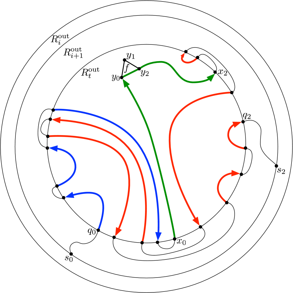
(a)
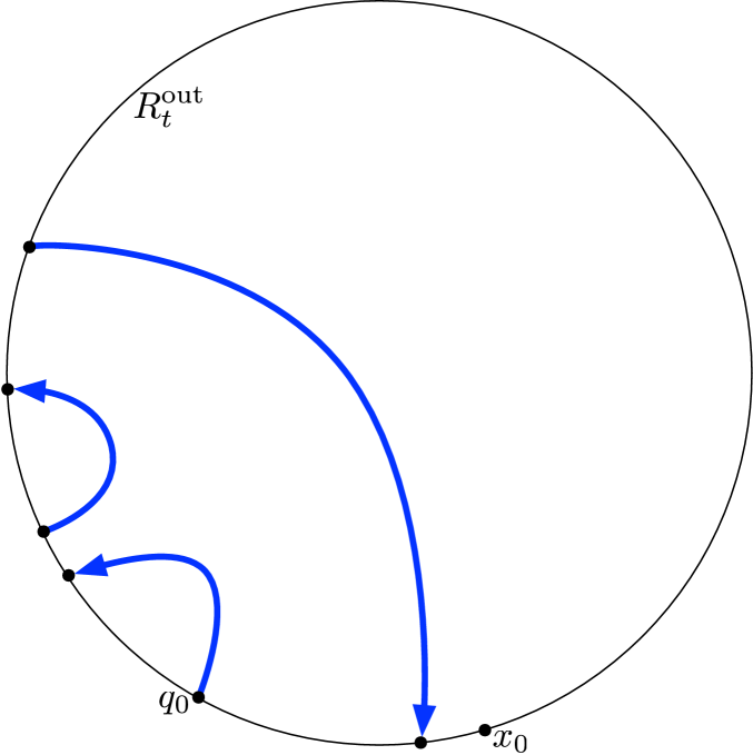
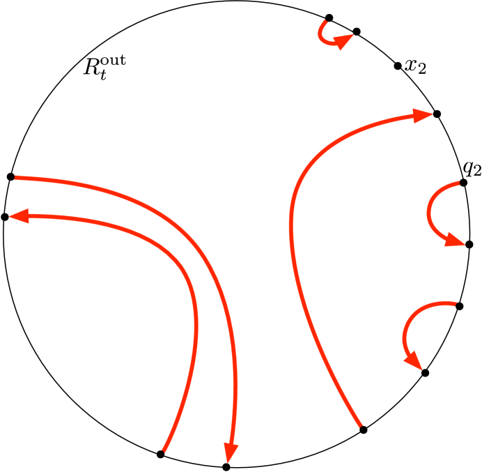
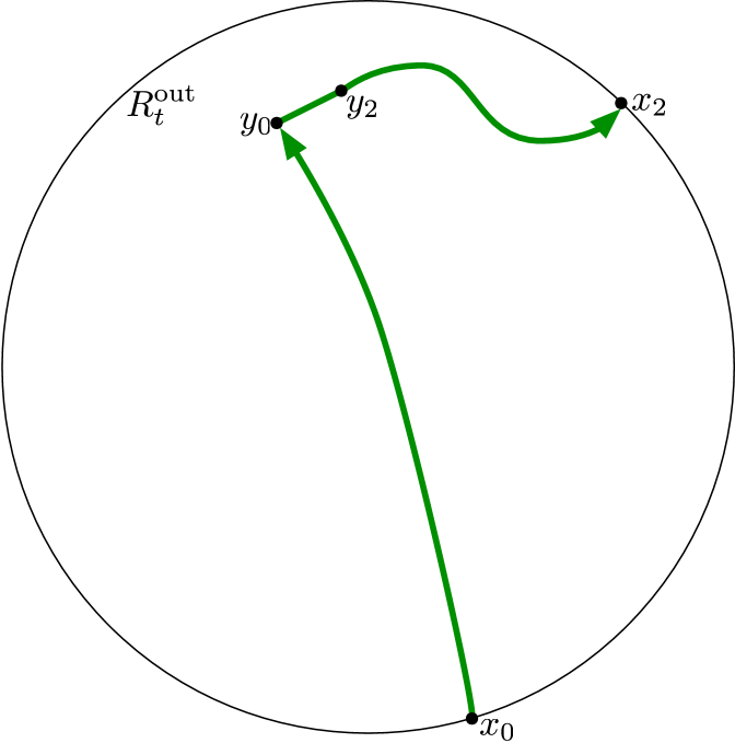
(b)	(c)	(d)

Figure 6: (a) The projection of a site-centroid-site chord $C^{\star}=\overrightarrow{s_{j}y_{j}y_{j-1}s_{j-1}}$ of $R_{i+1}^{\operatorname{out}}$ onto $R_{t}^{\operatorname{out}}$ yields a set $\mathcal{C}$ of chords of $R_{t}^{\operatorname{out}}$, partitioned into three classes. Let $q_{j},x_{j}$ and $q_{j-1},x_{j-1}$ be the first and last $\partial R_{t}$-vertices on the $s_{j}$-$y_{j}$ and $s_{j-1}$-$y_{j-1}$ paths. (b) $\mathcal{C}_{1}$: all chords in $T_{q_{j}}^{R_{t}}[x_{j}]$. (c) $\mathcal{C}_{2}$: all chords in $T_{q_{j-1}}^{R_{t}}[x_{j-1}]$. Their orientation is the reverse of their counterparts in $C^{\star}$. (d) $\mathcal{C}_{3}$: the single chord $\overrightarrow{x_{j}y_{j}y_{j-1}x_{j-1}}$.

Luckily $\mathcal{C}$ has some structure. Let $(q_{j},x_{j})$ and $(q_{j-1},x_{j-1})$ be the first and last $\partial R_{t}$ vertices on the shortest $s_{j}$-$y_{j}$ and $s_{j-1}$-$y_{j-1}$ paths, respectively. (One or both of these pairs may not exist.) The chords of $\mathcal{C}$ are in one-to-one correspondence with the chords of $\mathcal{C}_{1}\cup\mathcal{C}_{2}\cup\mathcal{C}_{3}$, defined below, but as we will see, sometimes with their orientation reversed.

1. By definition $\mathcal{C}_{1}=C_{q_{j}}^{R_{t}}[x_{j}]$ contains all the chords on the path from $q_{j}$ to $x_{j}$, stored in part (D) of the data structure. Moreover, the orientation of $\mathcal{C}_{1}$ agrees with the orientation of $C^{\star}$. The blue chords of Figure 6(a) are isolated as $\mathcal{C}_{1}$ in Figure 6(b).

2. By definition $\mathcal{C}_{2}=C_{q_{j-1}}^{R_{t}}[x_{j-1}]$ contains all the chords on the path from $q_{j-1}$ to $x_{j-1}$. The red chords of $\mathcal{C}$ in Figure 6(a) are represented by chords $\mathcal{C}_{2}$, but with reversed orientation. Figure 6(c) depicts $\mathcal{C}_{2}$.

3. This is the singleton set containing the oriented chord $\overrightarrow{x_{j}x_{j-1}}$ consisting of the shortest $x_{j}$-$y_{j}$ and $x_{j-1}$-$y_{j-1}$ paths and the edge $\{y_{j},y_{j-1}\}$.

The chord-set $\mathcal{C}$ partitions $R_{t}^{\operatorname{out}}$ into a piece-set $\mathcal{P}$, with one such piece $P\in\mathcal{P}$ containing $v$. (Remember that $v$ is not on $C^{\star}$.) We can also consider the piece-sets $\mathcal{P}_{1},\mathcal{P}_{2},\mathcal{P}_{3}$ generated by $\mathcal{C}_{1},\mathcal{C}_{2},\mathcal{C}_{3}$. Let $P_{1}\in\mathcal{P}_{1},P_{2}\in\mathcal{P}_{2},P_{3}\in\mathcal{P}_{3}$ be the pieces containing $v$. Since, ignoring orientation, $\mathcal{C}=\mathcal{C}_{1}\cup\mathcal{C}_{2}\cup\mathcal{C}_{3}$, it must be that $P=P_{1}\cap P_{2}\cap P_{3}$. In order to determine whether $v$ is to the right of $C^{\star}$, it suffices to find some chord $C\in\mathcal{C}$ bounding $P$ and ask whether $v$ is to the right of $C$. Thus, $C$ must also be on the boundary of one of $P_{1},P_{2},$ or $P_{3}$.

The high-level strategy of $\boldsymbol{\mathsf{ChordIndicator}}$ is as follows. First, we will find some piece $P_{1}^{\prime}\in\mathcal{P}_{q_{j}}^{R_{t}}$ that is contained in $P_{1}$ using the procedure $\boldsymbol{\mathsf{PieceSearch}}$ described below, in Section 4.4.1. The chords of $\mathcal{C}_{1}$ bounding $P_{1}$ are precisely the maximal chords in $\mathcal{C}_{1}$ from vantage $P_{1}^{\prime}$. Using $\boldsymbol{\mathsf{MaximalChord}}$ (part (D)) we will find a candidate chord $C_{1}\in\mathcal{C}_{1}$, and one edge $e$ on the boundary cycle of $\partial R_{t}$ occluded by $C_{1}$ from vantage $P_{1}^{\prime}$. Turning to $\mathcal{C}_{2}$, we use $\boldsymbol{\mathsf{AdjacentPiece}}$ to find the piece $P_{e}\in\mathcal{P}_{q_{j-1}}^{R_{t}}$ adjacent to $e$. Then, using $\boldsymbol{\mathsf{PieceSearch}}$ and $\boldsymbol{\mathsf{MaximalChord}}$ again, we find a $P_{2}^{\prime}\in\mathcal{P}_{q_{j-1}}^{R_{t}}$ contained in $P_{2}$ and the maximal chord $C_{2}$ occluding $P_{e}$ from vantage $P_{2}^{\prime}$. Let $C_{3}$ be the singleton chord in $\mathcal{C}_{3}$. We determine the “best” chord $C_{\ell}\in\{C_{1},C_{2},C_{3}\}$, decide whether $v$ lies to the right of $C_{\ell}$, and return this answer if $\ell\in\{1,3\}$ or reverse it if $\ell=2$. Recall that chords in $\mathcal{C}_{2}$ have the opposite orientation as their counterparts in $\mathcal{C}$.

$\boldsymbol{\mathsf{PieceSearch}}$ is presented in Section 4.4.1 and $\boldsymbol{\mathsf{ChordIndicator}}$ in Section 4.4.2.

4.4.1 $\boldsymbol{\mathsf{PieceSearch}}$

We are given a region $R_{t}$, a vertex $v\in R_{t}^{\operatorname{out}}\cap R_{t+1}$, and two vertices $q,x\in\partial R_{t}$. We must locate any piece $P^{\prime}\in\mathcal{P}_{q}^{R_{t}}$ that is contained in the unique piece $P\in\mathcal{P}_{q}^{R_{t}}[x]$ containing $v$. The first thing we do is find the last $\partial R_{t}$ vertex $z$ on the shortest path from $q$ to $v$, which can be found with a call to $\boldsymbol{\mathsf{PointLocate}}$ on $\mathrm{VD}^{*}_{\operatorname{out}}(q,R_{t})$. (This uses parts (A,C,E) of the data structure.) The shortest path from $z$ to $v$ cannot cross any chord in $\mathcal{C}_{q}^{R_{t}}[x]$ (since they are part of a shortest path), but it can coincide with a prefix of some chord in $\mathcal{C}_{q}^{R_{t}}[x]$. Thus, if no chord of $\mathcal{C}_{q}^{R_{t}}[x]$ is incident to $z$, then we are free to return any piece containing $z$. (There may be multiple options if $z$ is an endpoint of a chord in $\mathcal{C}_{q}^{R_{t}}$. This case is depicted in Figure 7. When $z=z_{0}$, we know that $v\in P_{5}\cup\cdots\cup P_{9}$ and return any piece containing $z$.) In general $z$ may be incident to up to two chords $C_{1},C_{2}\in\mathcal{C}_{q}^{R_{t}}[x]$. (This occurs when the shortest $q$-$x$ path touches $\partial R_{t}$ at $z$ without leaving $R_{t}^{\operatorname{out}}$.) In this case we determine which side of $C_{1}$ and $C_{2}$ $v$ is on (using parts (A) and (E) of the data structure; see Lemma 4.3 in Section 4.4.3 for details) and return the appropriate piece adjacent to $C_{1}$ or $C_{2}$. This case is depicted in Figure 7 with $z=z_{1}$; the three possible answers coincide with $v\in\{v_{1},v_{2},v_{3}\}$.

Algorithm 5 $\boldsymbol{\mathsf{PieceSearch}}(R_{t},q,x,v)$

1:A region $R_{t}$, two vertices $q,x\in\partial R_{t}$, and a vertex $v$ not on the $q$-to-$x$ shortest path in $G$.

2:A piece $P^{\prime}\in\mathcal{P}_{q}^{R_{t}}$, which is a subpiece of the unique piece $P\in\mathcal{P}_{q}^{R_{t}}[x]$ containing $v$.

3:$z\leftarrow\boldsymbol{\mathsf{PointLocate}}(\mathrm{VD}^{*}_{\operatorname{out}}(q,R_{t}),v)$ $\triangleright$ Uses parts (A,C,E) of the data structure

4:if $z$ is not the endpoint of any chord in $\mathcal{C}_{q}^{R_{t}}[x]$ then

5:     return any piece in $\mathcal{P}_{q}^{R_{t}}$ containing $z$.

6:end if

7:$C_{1},C_{2}\leftarrow$ two chords in $\mathcal{C}_{q}^{R_{t}}[x]$ adjacent to $z$ ($C_{2}$ may be Null)

8:Determine whether $v$ is to the left or right of $C_{1}$ and $C_{2}$. $\triangleright$ Part (A); see Lemma 4.3

9:return a piece adjacent to $C_{1}$ or $C_{2}$ that respects the queries of Line 6.

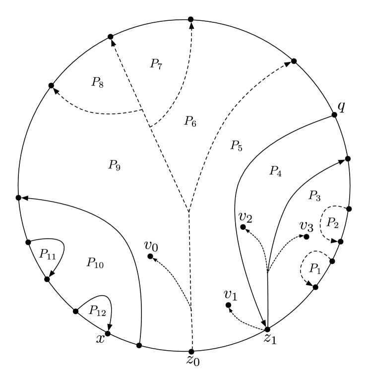
Figure 7: Solid chords are in $\mathcal{C}_{q}^{R_{t}}[x]$. Dashed chords are in $\mathcal{C}_{q}^{R_{t}}$ but not $\mathcal{C}_{q}^{R_{t}}[x]$. When $z=z_{0},v=v_{0}$, the piece in $\mathcal{P}_{q}^{R_{t}}[x]$ containing $v$ is the union of $P_{5}$–$P_{9}$. $\boldsymbol{\mathsf{PieceSearch}}$ reports any piece containing $z_{0}$. When $z=z_{1},v\in\{v_{1},v_{2},v_{3}\}$, $z$ is incident to two chords $C_{1},C_{2}$. $\boldsymbol{\mathsf{PieceSearch}}$ decides which side of $C_{1},C_{2}$ $v$ is on (see Lemma 4.3), and returns the appropriate piece adjacent to $C_{1}$ or $C_{2}$.

4.4.2 $\boldsymbol{\mathsf{ChordIndicator}}$

Let us walk through the $\boldsymbol{\mathsf{ChordIndicator}}$ function. If $C^{\star}=\overrightarrow{s_{j}y_{j}y_{j-1}s_{j-1}}$ does not touch the interior of $R_{t}^{\operatorname{out}}$ then the left-right relationship between $C^{\star}$ and $v\not\in R_{t}$ is known, and stored in part (E) of the data structure. If this is the case the answer is returned immediately, at Line 3. A relatively simple case is when $\mathcal{C}_{1}$ and $\mathcal{C}_{2}$ are empty, and $\mathcal{C}=\mathcal{C}_{3}$ consists of just one chord $C_{3}=\overrightarrow{x_{j}y_{j}y_{j-1}x_{j-1}}$. We determine whether $v$ is to the right or left of $C_{3}$ and return this answer (Line 8). (Lemma 4.3 in Section 4.4.3 explains how to test whether $v$ is to one side of a chord.) Thus, without loss of generality we can assume $\mathcal{C}_{1}\neq\emptyset$ and $\mathcal{C}_{2}$ may or may not be empty.

Recall that $P_{1}$ is $v$’s piece in $\mathcal{P}_{q_{j}}^{R_{t}}[x_{j}]$. Using $\boldsymbol{\mathsf{PieceSearch}}$ we find a piece $P_{1}^{\prime}\subseteq P_{1}$ in the more refined partition $\mathcal{P}_{q_{j}}^{R_{t}}$ and find a $\boldsymbol{\mathsf{MaximalChord}}$ $C_{1}\in\mathcal{C}_{1}$ from vantage $P_{1}^{\prime}$, and hence from vantage $v$ as well. We regard $\partial R_{t}$ as circularly ordered according to a clockwise walk around the hole on $\partial R_{t}$ in $R_{t}^{\operatorname{out}}$. The chord $C_{1}$ occludes an interval $I_{1}$ of $\partial R_{t}$ from vantage $v$. If $C_{1}$ is not one of the chords bounding $P$, then $C_{3}$ or some $C_{2}\in\mathcal{C}_{2}$ must occlude a superset of $I_{2}$, so we will attempt to find such a $C_{2}$, as follows.

Let $e$ be the first edge on the boundary cycle occluded by $C_{1}$, i.e., $e$ joins the first two elements of $I_{1}$. Using $\boldsymbol{\mathsf{AdjacentPiece}}$ we find the unique piece $P_{e}\in\mathcal{P}_{q_{j-1}}^{R_{t}}$ with $e$ on its boundary. Using $\boldsymbol{\mathsf{PieceSearch}}$ again we find $P_{2}^{\prime}\in\mathcal{P}_{q_{j-1}}^{R_{t}}$ contained in $P_{2}$, and using $\boldsymbol{\mathsf{MaximalChord}}$ again, we find the maximal chord $C_{2}\in\mathcal{C}_{2}$ that occludes $P_{e}$ from vantage $P_{2}^{\prime}$, and hence from vantage $v$ as well. Observe that since all chords in $\mathcal{C}_{2}$ are vertex-disjoint from $C_{1}$, if $C_{2}\neq$ Null then $C_{2}$ must occlude a strictly larger interval $I_{2}\supset I_{1}$ of $\partial R_{t}$. (If $C_{2}$ is Null then $I_{2}=\emptyset$.) It may be that $C_{1}$ and $C_{2}$ are both not on the boundary of $P$, but the only way that could occur is if $C_{3}\in\mathcal{C}_{3}$ occludes a superset of $I_{1}$ and $I_{2}$ on the boundary $\partial R_{t}$. We check whether $v$ lies to the right or left of $C_{3}$ and let $I_{3}$ be the interval of $\partial R_{t}$ occluded by $C_{3}$ from vantage $v$. If $I_{3}$ does not cover $e$, then we cannot conclude that $C_{3}$ is superior than $C_{1}/C_{2}$. Thus, we find the chord $C_{\ell}\in\{C_{1},C_{2},C_{3}\}$ that covers $e$ and maximizes $|I_{\ell}|$. $C_{\ell}$ must be on the boundary of $P$, so the left-right relationship between $v$ and $C^{\star}$ is exactly the same as the left-right relationship between $v$ and $C_{\ell}$, if $\ell\in\{1,3\}$, and the reverse of this relationshp if $\ell=2$ since chords in $\mathcal{C}_{2}$ have the opposite orientation as their subpath counterparts in $C^{\star}$. Figure 8 illustrates how $\ell$ could take on all three values.

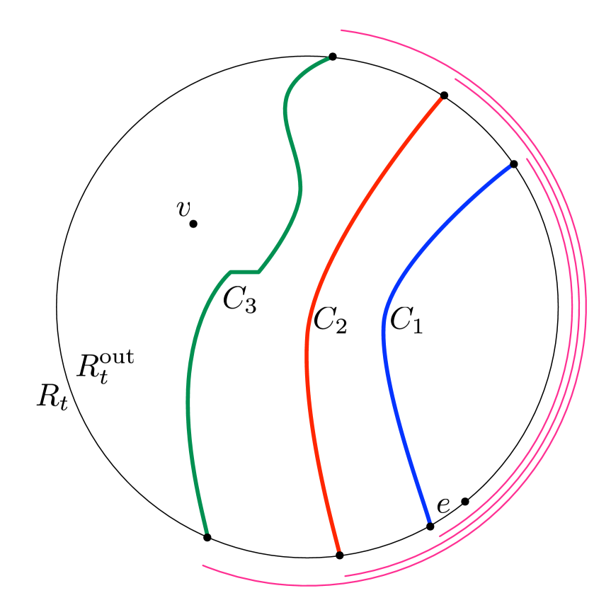
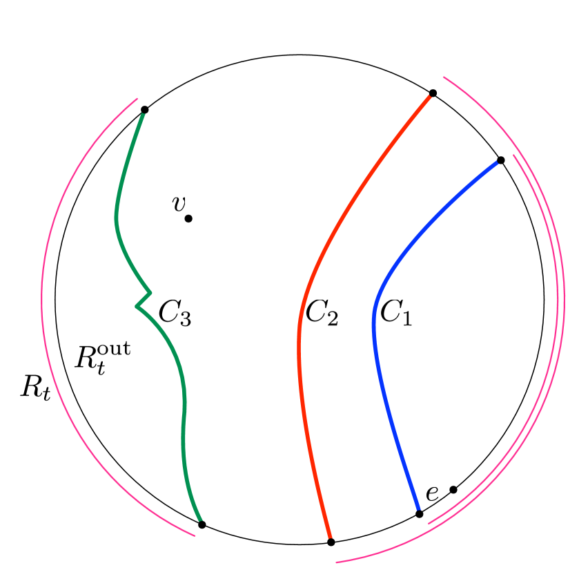
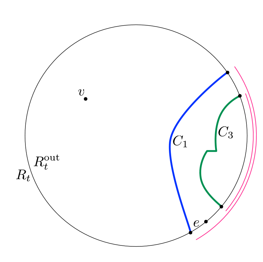
(a)	(b)	(c)

Figure 8: The intervals $I_{1},I_{2},I_{3}$ are represented as pink circular arcs. In (a) $C_{2}$ exists and $C_{3}$ is better than $C_{1},C_{2}$ since $I_{3}\supset I_{2}\supset I_{1}$. In (b) $C_{2}$ exists, but $C_{3}$ occludes an interval $I_{3}$ that does not contain $e$, so $C_{2}$ is the best chord. In (c) $C_{2}$ is Null, and $C_{3}$ does not occlude $e$ from $v$, so $C_{1}$ is the only eligible chord. (In the figure $I_{3}\subset I_{1}$ but it could also be as in (b), with $I_{3}$ disjoint from $I_{1}$.)

Algorithm 6 $\boldsymbol{\mathsf{ChordIndicator}}(\mathrm{VD}^{*}_{\operatorname{out}}(u_{i},R_{i+1}),v,f^{*},j)$

1:The dual representation $\mathrm{VD}^{*}_{\operatorname{out}}=\mathrm{VD}^{*}_{\operatorname{out}}(u_{i},R_{i+1})$ of a Voronoi diagram, a centroid $f^{*}$ in $\mathrm{VD}^{*}_{\operatorname{out}}$ with face $f$ on vertices $y_{0},y_{1},y_{2}$, which are in the Voronoi cells of $s_{0},s_{1},s_{2}$, an index $j\in\{0,1,2\}$, and a vertex $v\in R_{i+1}^{\operatorname{out}}$ that does not lie on the site-centroid-site chord $C^{\star}=\overrightarrow{s_{j}y_{j}y_{j-1}s_{j-1}}$.

2:True if $v$ lies to the right of $C^{\star}$, and False otherwise.

3:$R_{t}\leftarrow$ the ancestor of $R_{i}$ s.t. $v\notin R_{t},v\in R_{t+1}$. $\mathcal{C}$ is the projection of $C^{\star}$ onto $R_{t}^{\operatorname{out}}$.

4:if the left/right relationship between $R_{t}^{\operatorname{out}}$ and $C^{\star}=\overrightarrow{s_{j}y_{j}y_{j-1}s_{j-1}}$ is known then

5:     return stored True/False answer. $\triangleright$ Part (E)

6:end if$\triangleright$ (It follows that $C^{\star}$ crosses $\partial R_{t}$ and that $\mathcal{C}\neq\emptyset$)

7:$(q_{j},x_{j})\leftarrow$ first and last $\partial R_{t}$-vertices on shortest $s_{j}$-$y_{j}$ path. $\triangleright$ Part (E)

8:$(q_{j-1},x_{j-1})\leftarrow$ first and last $\partial R_{t}$-vertices on shortest $s_{j-1}$-$y_{j-1}$ path. $\triangleright$ Part (E)

9:if $\mathcal{C}_{1}=\mathcal{C}_{2}=\emptyset$ then

10:     return True if $v$ is to the right of the $\mathcal{C}_{3}$-chord $\overrightarrow{x_{j}y_{j}y_{j-1}x_{j-1}}$, or False otherwise.

11:end if$\triangleright$ W.l.o.g., continue under the assumption that $\mathcal{C}_{1}\neq\emptyset$.

12:$P_{1}^{\prime}\leftarrow\boldsymbol{\mathsf{PieceSearch}}(R_{t},q_{j},x_{j},v)$ $\triangleright$ Uses parts (A,C)

13:$C_{1}\leftarrow\boldsymbol{\mathsf{MaximalChord}}(R_{t},q_{j},x_{j},P_{1}^{\prime},\perp)$ $\triangleright$ Part (D)

14:$I_{1}\leftarrow$ the clockwise interval of hole $\partial R_{t}$ occluded by $C_{1}$ from vantage $v$.

15:$e\leftarrow$ edge joining first two elements of $I_{1}$.

16:$P_{e}\leftarrow\boldsymbol{\mathsf{AdjacentPiece}}(R_{t},q_{j-1},e)$ $\triangleright$ Part (D)

17:$P_{2}^{\prime}\leftarrow\boldsymbol{\mathsf{PieceSearch}}(R_{t},q_{j-1},x_{j-1},v)$ $\triangleright$ Uses parts (A,C)

18:$C_{2}\leftarrow\boldsymbol{\mathsf{MaximalChord}}(R_{t},q_{j-1},x_{j-1},P_{2}^{\prime},P_{e})$ $\triangleright$ Part (D); may return Null

19:$I_{2}\leftarrow$ the clockwise interval of hole $\partial R_{t}$ occluded by $C_{2}$ from vantage $v$. $\triangleright$ $\emptyset$ if $C_{2}=$ Null

20:$C_{3}\leftarrow$ single chord in $\mathcal{C}_{3}$, if any. $\triangleright$ May be Null

21:$I_{3}\leftarrow$ the clockwise interval of hole $\partial R_{t}$ occluded by $C_{3}$ from vantage $v$. $\triangleright$ $\emptyset$ if $C_{3}=$ Null

22:$\ell\leftarrow$ index such that $I_{\ell}$ covers $e$, and $|I_{\ell}|$ is maximum.

23:if $v$ is to the right of $C_{\ell}$ and $\ell\in\{1,3\}$ or $v$ is to the left of $C_{\ell}$ and $\ell=2$ then

24:     return True

25:end if

26:return False

4.4.3 Side Queries

Lemma 4.3 explains how we test whether $v$ is to the right or left of a chord, which is used in both $\boldsymbol{\mathsf{PieceSearch}}$ and $\boldsymbol{\mathsf{ChordIndicator}}$.

Lemma 4.3.

For any $C\in\mathcal{C}_{1}\cup\mathcal{C}_{2}\cup\mathcal{C}_{3}$ and $v$ not on $C$, we can test whether $v$ lies to the right or left of $C$ in $O(\kappa\log\log n)$ time, using parts (A) and (E) of the data structure.

Proof.

There are several cases.

Case 1.

Suppose that $C=\overrightarrow{c_{0}c_{1}}\in\mathcal{C}_{1}\cup\mathcal{C}_{2}$ corresponds to the shortest path from $c_{0}$ to $c_{1}$ in $R_{t}^{\operatorname{out}}$, $c_{0},c_{1}\in\partial R_{t}$. Let $c_{0}^{\prime},c_{1}^{\prime}$ be pendant vertices attached to $c_{0},c_{1}$ embedded inside the face of $R_{t}^{\operatorname{out}}$ bounded by $\partial R_{t}$. The shortest $c_{0}^{\prime}$-$v$ paths and $c_{0}^{\prime}$-$c_{1}^{\prime}$ paths branch at some point. We ask the MSSP structure (part (A)) for the least common ancestor, $w$, of $v$ and $c_{1}^{\prime}$ in the shortcutted SSSP tree rooted at $c_{0}^{\prime}$. This query also returns the two tree edges $e_{v},e_{c_{1}^{\prime}}$ leading to $v$ and $c_{1}^{\prime}$, respectively. Let $e_{w}$ be the edge connecting $w$ to its parent. If the clockwise order around $w$ is $e_{w},e_{c_{1}^{\prime}},e_{v}$ then $v$ lies to the right of $\overrightarrow{c_{0}c_{1}}$; otherwise it lies to the left. Note that if the shortest $c_{0}^{\prime}$-$c_{1}^{\prime}$ and $c_{0}^{\prime}$-$v$ paths in $G$ branch at a point in $R_{t+1}^{\operatorname{out}}$, then $w$ will be the nearest ancestor of the branchpoint on $\partial R_{t+1}$ and one or both of $e_{v},e_{c_{1}^{\prime}}$ may be “shortcut” edges in the MSSP structure. See Figure 9(a) for a depiction of this case.

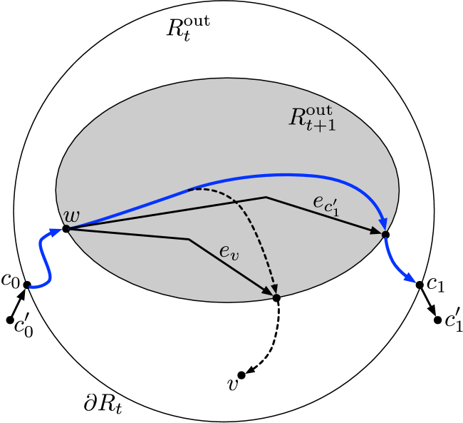
(a)
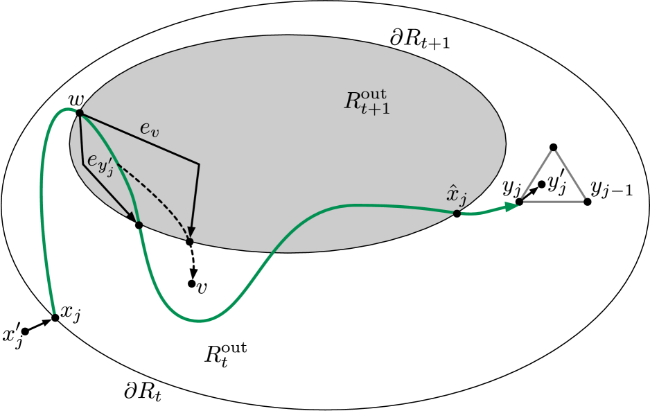
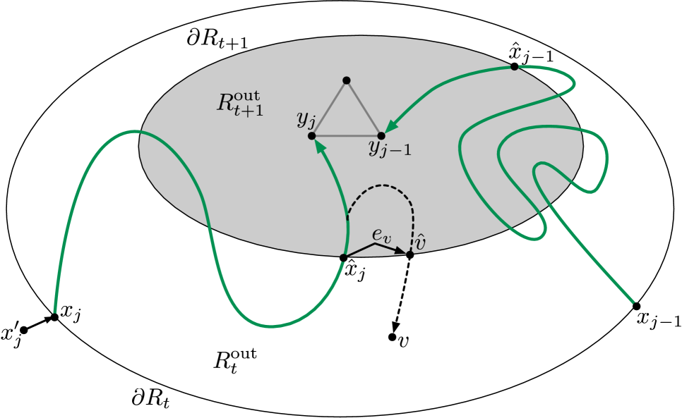
(b)	(c)

Figure 9: (a) The chord $C\in\mathcal{C}_{1}\cup\mathcal{C}_{2}$ corresponds to a shortest path, which may pass through $R_{t+1}^{\operatorname{out}}$, in which case it is represented in the MSSP structure with shortcut edges (solid, angular edges). (b) The chord $C=\overrightarrow{x_{j}y_{j}y_{j-1}x_{j-1}}$ is in $\mathcal{C}_{3}$, and $f$ lies in $R_{t}^{\operatorname{out}}\cap R_{t+1}$. This is handled similarly to (a). (c) Here $f$ lies in $R_{t+1}^{\operatorname{out}}$, $\hat{x}_{j},\hat{x}_{j-1}$ are the last $\partial R_{t+1}$ vertices on the $s_{j}$-$y_{j}$ and $s_{j-1}$-$y_{j-1}$ paths. If the shortest $x_{j}^{\prime}$-$\hat{x}_{j}$ and $x_{j}^{\prime}$-$v$ paths branch, we can answer the query as in (b). If $x_{j}^{\prime}$-$\hat{x}_{j}$ is a prefix of $x_{j}^{\prime}$-$v$, $e_{v}=(\hat{x}_{j},\hat{v})$, and $\hat{v}\in\partial R_{t+1}$, then we can use the clockwise order of $\hat{x}_{j},\hat{v},\hat{x}_{j-1}$ around the hole on $\partial R_{t+1}$ to determine whether $v$ lies to the right of $C$. (Not depicted: the case when $\hat{v}\not\in\partial R_{t+1}$.)

Case 2.

Now suppose $C=\overrightarrow{x_{j}y_{j}y_{j-1}x_{j-1}}$ is the one chord in $\mathcal{C}_{3}$. Consider the following distance function $\hat{d}$ for vertices in $z\in R_{t}^{\operatorname{out}}$:

$$\hat{d}(z)=\min\Big{\{}\operatorname{dist}_{G}(u_{i},x_{j})+\operatorname{dist}_{G}(x_{j},z),\;\;\operatorname{dist}_{G}(u_{i},x_{j-1})+\operatorname{dist}_{G}(x_{j-1},z)\Big{\}}.$$

Observe that the terms involving $u_{i}$ are stored in part (E) and, if $z\in R_{t}^{\operatorname{out}}\cap R_{t+1}$, the other terms can be queried in $O(\kappa\log\log n)$ time using part (A). It follows that the shortest path forest w.r.t. $\hat{d}$ has two trees, rooted at $x_{j}$ and $x_{j-1}$. Using part (A) of the data structure we compute $\hat{d}(v)$, which reveals the $j^{\star}\in\{j,j-1\}$ such that $v$ is in $x_{j^{\star}}$’s tree. At this point we break into two cases, depending on whether $f$ is in $R_{t}^{\operatorname{out}}\cap R_{t+1}$, or in $R_{t+1}^{\operatorname{out}}$. We assume $j^{\star}=j$ without loss of generality and depict only this case in Figure 9(b,c).

Case 2a.

Suppose that $f$ is in $R_{t}^{\operatorname{out}}\cap R_{t+1}$. Let $y^{\prime}_{j}$ be a pendant vertex attached to $y_{j}$ embedded inside $f$ and let $x_{j}^{\prime}$ be a pendant attached to $x_{j}$ embedded in the face on $\partial R_{t}$. The shortest $x_{j}^{\prime}$-$y_{j}^{\prime}$ and $x_{j}^{\prime}$-$v$ paths diverge at some point. We query the MSSP structure (part (A)) to get the least common ancestor $w$ of $y_{j}^{\prime}$ and $v$ and the three edges $e_{y_{j}^{\prime}},e_{v},e_{w}$ around $w$, then determine the left/right relationship as in Case 1. (If $j^{\star}=j-1$ then we would reverse the answer due to the reversed orientation of the $x_{j-1}$-$y_{j-1}$ subpath w.r.t. $C$.) Once again, some of $e_{y_{j}^{\prime}},e_{v},e_{w}$ may be shortcut edges between $\partial R_{t+1}$-vertices or artificial pendant edges. See Figure 9(b)

Case 2b.

Now suppose $f$ lies in $R_{t+1}^{\operatorname{out}}$. We get from part (E) the last vertices $\hat{x}_{j},\hat{x}_{j-1}\in\partial R_{t+1}$ that lie on the $s_{j}$-$y_{j}$ and $s_{j-1}$-$y_{j-1}$ shortest paths. We ask the MSSP structure of part (A) for the least common ancestor $w$ of $\hat{x}_{j}$ and $v$ in the shortcutted SSSP tree rooted at $x_{j}^{\prime}$, and also get the three incident edges $e_{\hat{x}_{j}},e_{v},e_{w}$. The edges $e_{v}$ and $e_{w}$ exist and are different, but $e_{\hat{x}_{j}}$ may not exist if $w=\hat{x}_{j}$, i.e., if $v$ is a descendant of $\hat{x}_{j}$. If all three edges $\{e_{\hat{x}_{j}},e_{v},e_{w}\}$ exist we can determine whether $v$ lies to the right of $C$ as in Case 1 or 2a.

Case 2b(i).

Suppose $w=\hat{x}_{j}$ and $e_{\hat{x}_{j}}$ does not exist. Let $e_{v}=(\hat{x}_{j},\hat{v})$. If $\hat{v}\in\partial R_{t+1}$ then $e_{v}$ represents a path that is completely contained in $R_{t+1}^{\operatorname{out}}$. Thus, if we walk clockwise around the hole of $R_{t+1}^{\operatorname{out}}$ on $\partial R_{t+1}$ and encounter $\hat{x}_{j},\hat{v},\hat{x}_{j-1}$ in that order then $v$ lies to the right of $C$, and if we encounter them in the reverse order then $v$ lies to the left of $C$. See Figure 9(c).

Case 2b(ii).

Finally, suppose $\hat{v}\not\in\partial R_{t+1}$ and $e_{v}=(\hat{x}_{j},\hat{v})$ is a normal edge in $G$. Redefine $e_{\hat{x}_{j}}$ to be the first edge on the path from $\hat{x}_{j}$ to $y_{j}$. Now we can determine if $v$ is to the right of $C$ by looking at the clockwise order of $e_{w},e_{v},e_{\hat{x}_{j}}$ around $\hat{x}_{j}$. ∎

As pointed out in Remark 1, Lemma 2.1 does not immediately imply that Line 6 of $\boldsymbol{\mathsf{SitePathIndicator}}$ and Line 1 of $\boldsymbol{\mathsf{PieceSearch}}$ can be implemented efficiently. Gawrychowski et al.’s [20] implementation of $\boldsymbol{\mathsf{PointLocate}}$ requires MSSP access to $R_{t}^{\operatorname{out}}$, whereas part (A) only lets us query vertices in $R_{t}^{\operatorname{out}}\cap R_{t+1}$. Gawrychowski et al.’s algorithm is identical to $\boldsymbol{\mathsf{CentroidSearch}}$, except that $\boldsymbol{\mathsf{Navigation}}$ is done directly with MSSP structures. Suppose we are currently at $f^{*}$ in the centroid decomposition, with $y_{j},s_{j}$ defined as usual. Gawrychowski’s algorithm finds $j$ minimizing $\omega(s_{j})+\operatorname{dist}_{R_{t}^{\operatorname{out}}}(s_{j},v)$ using three distance queries to the MSSP structure, then decides whether the $s_{j}^{\prime}$-$v$ shortest path is a prefix of the $s_{j}^{\prime}$-$y_{j}^{\prime}$ shortest path, and if not, which direction it branches in. If $f$ is in $R_{t}^{\operatorname{out}}\cap R_{t+1}$ we can proceed exactly as in Gawrychowski et al. [20]. If not, we retrieve from part (E) the last vertex $\hat{x}$ of $\partial R_{t+1}$ on the $s_{j}$-$y_{j}$ shortest path, use $\hat{x}$ in lieu of $y_{j}^{\prime}$ for the LCA queries, and tell whether the $s_{j}^{\prime}$-$v$ path branches to the right exactly as in Lemma 4.3, Case 2b.

5 Analysis

This section constitutes a proof of the claims of Theorem 1.1 concerning space complexity and query time; refer to Appendix C for an efficient construction algorithm.

Combining Lemmas 2.1 and 2.2 (see Section 4.4.3), $\boldsymbol{\mathsf{PointLocate}}$ runs in $O(\kappa\log n\log\log n)$ time. Together with Lemma 4.3 it follows that $\boldsymbol{\mathsf{PieceSearch}}$ also takes $O(\kappa\log n\log\log n)$ time. $\boldsymbol{\mathsf{SitePathIndicator}}$ uses $\boldsymbol{\mathsf{PointLocate}}$, the MSSP structure, and $O(1)$-time tree operations on $T_{q}^{R_{i}}$ and the $\vec{r}$-hierarchy like least common ancestors and level ancestors [22, 4, 5, 21]. Thus $\boldsymbol{\mathsf{SitePathIndicator}}$ also takes $O(\kappa\log n\log\log n)$ time. The calls to $\boldsymbol{\mathsf{MaximalChord}}$ and $\boldsymbol{\mathsf{AdjacentPiece}}$ in $\boldsymbol{\mathsf{ChordIndicator}}$ take $O(\log n\log\log n)$ time by Lemma 4.1, and testing which side of a chord $v$ lies on takes $O(\kappa\log\log n)$ time by Lemma 4.3. The bottleneck in $\boldsymbol{\mathsf{ChordIndicator}}$ is still $\boldsymbol{\mathsf{PieceSearch}}$, which takes $O(\kappa\log n\log\log n)$ time. The only non-trivial parts of $\boldsymbol{\mathsf{Navigation}}$ are calls to $\boldsymbol{\mathsf{SitePathIndicator}}$ and $\boldsymbol{\mathsf{ChordIndicator}}$, so it, too, takes $O(\kappa\log n\log\log n)$ time.

An initial call to $\boldsymbol{\mathsf{CentroidSearch}}$ (Line 5 of $\boldsymbol{\mathsf{Dist}}$) generates at most $\log n$ recursive calls to $\boldsymbol{\mathsf{CentroidSearch}}$, culminating in the last recursive call making 1 or 2 calls to $\boldsymbol{\mathsf{Dist}}$ with the “$i$” parameter incremented. Excluding the cost of recursive calls to $\boldsymbol{\mathsf{Dist}}$, the cost of $\boldsymbol{\mathsf{CentroidSearch}}$ is dominated by calls to $\boldsymbol{\mathsf{Navigation}}$, i.e., an initial call to $\boldsymbol{\mathsf{CentroidSearch}}$ costs $\log n\cdot O(\kappa\log n\log\log n)=O(\kappa\log^{2}n\log\log n)$ time. Let $T(i)$ be the cost of a call to $\boldsymbol{\mathsf{Dist}}(u_{i},v,R_{i})$. We have

$$T(m-1) =O(\kappa\log\log n) \boldsymbol{\mathsf{Dist}}$$ returns at Line 2 with one MSSP query

$$T(i) =2T(i+1)+O(\kappa\log^{2}n\log\log n)$$

It follows that the time to answer a distance query is $T(0)=O(2^{m}\cdot\kappa\log^{2}n\log\log n)$.

The space complexity of each part of the data structure is as follows. (A) is $O(\kappa mn^{1+1/m+1/\kappa})$ by Lemma 2.1 and the fact that $r_{i+1}/r_{i}=n^{1/m}$. (B) is $O(mn^{1+1/(2m)})$ since $\sqrt{r_{i+1}/r_{i}}=n^{1/(2m)}$. (C) is $O(mn)$ since $\sum_{i}n/r_{i}\cdot(\sqrt{r_{i}})^{2}=O(mn)$. (D) is $O(mn\log n)$ by Lemma 4.2, and (E) is $O(m)$ times the space cost of (B) and (C), namely $O(m^{2}n^{1+1/(2m)})$. The bottleneck is (A).

We now explain how $m,\kappa$ can be selected to achieve the extreme space and query complexities claimed Theorem 1.1. To optimize for query time, pick $\kappa=m$ to be any function of $n$ that is $\omega(1)$ and $o(\log\log n)$. Then the query time is

$$O(2^{m}\kappa\log^{2}n\log\log n)=\log^{2+o(1)}n$$

and the space is

$$O(m\kappa n^{1+1/m+1/\kappa})=n^{1+o(1)}.$$

To optimize for space, choose $\kappa=\log n$ and $m$ to be a function that is $\omega(\log n/\log\log n)$ and $o(\log n)$. Then the space is

$$O\left(m\kappa n^{1+1/m+1/\kappa}\right)=o\left(n^{1+1/m}\log^{2}n\right)=n\cdot 2^{o(\log\log n)}\cdot\log^{2}n=n\log^{2+o(1)}n,$$

and the query time

$$O(2^{m}\kappa\log^{2}n\log\log n)=2^{o(\log n)}\log^{3}n\log\log n=n^{o(1)}.$$

5.1 Speeding Up the Query Time

Observe that the space of (B) is asymptotically smaller than the space of (A). Replace (B) with (B’)

1. (Voronoi Diagrams) Fix $i$, a region $R_{i}\in\mathcal{R}_{i}$ with ancestors $R_{i+1}\in\mathcal{R}_{i+1}$ and $R_{i+4}\in\mathcal{R}_{i+4}$. For each $q\in\partial R_{i}$ store

   $$\mathrm{VD}^{*}_{\operatorname{out}}(q,R_{i+1}) =\mathrm{VD}^{*}[R_{i+1}^{\operatorname{out}},\partial R_{i+1},\omega]$$

   $$\mathrm{VD}^{*}_{\operatorname{farout}}(q,R_{i+4}) =\mathrm{VD}^{*}[R_{i+4}^{\operatorname{out}},\partial R_{i+4},\omega] i<m-4$$ only if

   with $\omega(s)=\operatorname{dist}_{G}(q,s)$ in both cases. Over all regions $R_{i}$, the space for storing all $\mathrm{VD}^{*}_{\operatorname{out}}$s is $\tilde{O}(n^{1+1/(2m)})$ since $\sqrt{r_{i+1}/r_{i}}=n^{1/(2m)}$ and the space for $\mathrm{VD}^{*}_{\operatorname{farout}}$s is $\tilde{O}(n^{1+2/m})$ since $\sqrt{r_{i+4}/r_{i}}=n^{2/m}$.

Now the space for (A) is $\tilde{O}(n^{1+1/m+1/\kappa})=\tilde{O}(n^{1+2/m})$ is balanced with (B’). In the $\boldsymbol{\mathsf{Dist}}$ function we now consider three possibilities. If $v\in R_{i+1}$ we use part (A) to solve the problem without recursion. If $v\not\in R_{i+1}$ but $v\in R_{i+4}$ we proceed as usual, calling $\boldsymbol{\mathsf{CentroidSearch}}(\mathrm{VD}^{*}_{\operatorname{out}}(u_{i},R_{i+1}),v,\cdot)$, and if $v\not\in R_{i+4}$ we call $\boldsymbol{\mathsf{CentroidSearch}}(\mathrm{VD}^{*}_{\operatorname{farout}}(u_{i},R_{i+4}),v,\cdot)$. Observe that the depth of the $\boldsymbol{\mathsf{Dist}}$-recursion is now at most $t/4+O(1)<m/4+O(1)$, giving us a query time of $O(m2^{m/4}\log^{2}n\log\log n)$ with space $\tilde{O}(n^{1+2/m})$.

6 Conclusion

In this paper we have proven that it is possible to simultaneously achieve optimal space or query time, up to a $\log^{2+o(1)}n$ factor, and near-optimality in the other complexity measure, up to an $n^{o(1)}$ factor. The main open question in this area is whether there exists an exact distance oracle with $\tilde{O}(n)$ space and $\tilde{O}(1)$ query time. This will likely require new insights into the structure of shortest paths, which could lead, for example, to storing correlated versions of Voronoi diagrams more efficiently, or avoiding the binary branching recursion in our query algorithm.

Acknowledgements.

We thank Danny Sleator and Bob Tarjan for discussing update/query time tradeoffs for dynamic trees.

Appendix A MSSP via Euler Tour Trees (Proof of Lemma 2.1)

Let us recall the setup. We have a planar graph $H$ with a distinguished face $f$, and wish to answer $\operatorname{dist}_{H}(s,v)$ queries w.r.t. any $s$ on $f$ and $v\in V(H)$, and LCA queries w.r.t. any $s$ on $f$ and $u,v\in V(H)$. Klein [28] proved that if we move the source vertex $s$ around $f$ and record all the changes to the SSSP tree, every edge in $E(H)$ can be swapped into and out of the SSSP at most once, i.e., there are $O(|H|)$ updates in total. Thus, if we maintain the SSSP tree as the source travels around $f$ in a dynamic data structure with update time $U$ and query time $T$ (for distance and LCA queries), the universal persistence method for RAM data structures (see [12]) yields an MSSP data structure with space $O(|H|U)$ and query time $O(T\log\log|H|)$. Thus, to establish Lemma 2.1 it suffices to design a dynamic data structure for the following:

InitTree$(s^{\star},T)$:

Initialize a directed spanning tree $T$ from root $s^{\star}$. Edges have real-valued lengths.

Swap$(v,p,l)$:

Let $p^{\prime}$ be the parent of $v$; $p$ is not a descandant of $v$. Update $T\leftarrow T-\{(p^{\prime},v)\}\cup\{(p,v)\}$, where $(p^{\prime},v)$ has length $l$.

Dist$(v)$:

Return $\operatorname{dist}_{T}(s^{\star},v)$.

LCA$(u,v)$:

Return the LCA $y$ of $u$ and $v$ and the first edges $e_{u},e_{v}$ on the paths from $y$ to $u$ and from $y$ to $v$, respectively.

Here $s^{\star}$ will be a fixed root vertex embedded in $f$ with a single, weight-zero, out-edge to the current root on $f$. Changes to the SSSP tree are effected with $O(|H|)$ Swap operations. Klein [28] and Gawrychowski [20] use Sleator and Tarjan’s Link-Cut trees [37], which support Swap, Dist, and LCA (among other operations) in $O(\log|T|)$ time. We will use a souped-up version of Henzinger and King’s [23] Euler Tour trees. Let $\mathsf{ET}(T)$ be an Euler tour of $T$ starting and ending at $s^{\star}$. The elements of $\mathsf{ET}(T)$ are edges, and each edge of $T$ appears twice in $\mathsf{ET}(T)$, once in each direction. Each edge in $T$ points to its two occurrences in $\mathsf{ET}(T)$.

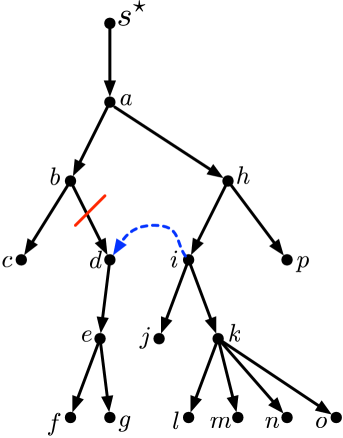
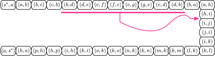
Figure 10: The effect of Swap$(d,i,\cdot)$ on the Euler Tour. The interval $((b,d),(d,e),\cdots,(e,d),(d,b))$ is spliced out and inserted between $(h,i)$ and $(i,j)$, and the elements $(b,d),(d,b)$ are renamed $(i,d),(d,i)$.

Suppose $T_{\operatorname{ante}}$ is the tree before a Swap operation and $T_{\operatorname{post}}$ the tree afterward. It is easy to see that $\mathsf{ET}(T_{\operatorname{post}})$ can be derived from $\mathsf{ET}(T_{\operatorname{ante}})$ by $O(1)$ splits and concatenates, and renaming the two elements corresponding to the swapped edge. See Figure 10. We will argue that the dynamic tree operations Swap, Dist, LCA can be implemented using the following list operations.

InitList$(L)$:

Initialize a list $L$ of weighted elements.

Split$(e_{0})$:

Element $e_{0}$ appears in some list $L$. Split $L$ immediately after element $e_{0}$, resulting in two lists.

Concatenate$(L_{0},L_{1})$:

Concatenate $L_{0}$ and $L_{1}$, resulting in one list.

Add$(e_{0},e_{1},\delta)$:

Here $e_{0},e_{1}$ are elements of the same list $L$. Add $\delta\in\mathbb{R}$ to the weight of all elements in $L$ between $e_{0}$ and $e_{1}$ inclusive.

Weight$(e_{0})$:

Return the weight of $e_{0}$.

RangeMin$(e_{0},e_{1})$:

Return the minimum-weight element between $e_{0}$ and $e_{1}$ inclusive. If there are multiple minima, return the first one.

To implement Dist and LCA we will actually use the list data structure with different weight functions. For Dist, the weight of an edge $(x,y)$ in $\mathsf{ET}(T)$ is $\operatorname{dist}_{T}(s^{\star},y)$. Thus, Dist is answered with a call to Weight. Each Swap$(v,p,l)$ is effected with $O(1)$ Split and Concatenate operations, renaming the elements of the swapped edge, as well as one Add$(e_{0},e_{1},\delta)$ operation. Here $(e_{0},\ldots,e_{1})$ is the sub-list corresponding to the subtree rooted at $v$, and $\delta=\operatorname{dist}_{T_{\operatorname{post}}}(s^{\star},v)-\operatorname{dist}_{T_{\operatorname{ante}}}(s^{\star},v)$ is the change in distance to $v$, and hence all descendants of $v$.

To handle LCA queries, we use the list data structure where the weight of $(x,y)$ is the depth of $y$ in $T$, i.e., the distance from $s^{\star}$ to $y$ under the unit length function. Once again, a Swap is implemented with $O(1)$ Split and Concatenate operations, and one Add operation. Consider an LCA$(u,v)$ query. Let $e_{0}=(p_{u},u),e_{1}=(p_{v},v)$ be the edges into $u$ and $v$ from their respective parents, and suppose that $e_{0}$ appears before $e_{1}$ in $\mathsf{ET}(T)$. A call to RangeMin$(e_{0},e_{1})$ returns the first edge $\hat{e}=(x,y)$ in the interval $(e_{0},\ldots,e_{1})$ minimizing the depth of $y$. It follows that $y$ is the LCA of $u$ and $v$. Furthermore, by the tiebreaking rule, if $\hat{e}\neq e_{0}$ then $\hat{e}=e_{u}$ is the (reversal of the) edge leading from $y$ towards $u$. If $\hat{e}=e_{0}$ then $v$ is a descendant of $u$ and $e_{u}$ does not exist. To find $e_{v}$, we retrieve the edge $\tilde{e}=(y,p_{y})$ in $\mathsf{ET}(T)$ from $y$ to its parent and let $\tilde{e}^{\prime}$ be its predecessor in $\mathsf{ET}(T)$. (Note that since $s^{\star}$ has degree 1, $\tilde{e},\tilde{e}^{\prime}$ always exist.) We call RangeMin$(e_{1},\tilde{e}^{\prime})$. Once again, by the tiebreaking rule it returns the first edge $e_{v}=(x^{\prime},y)$ incident to $y$ in $(e_{1},\ldots,\tilde{e}^{\prime})$, which is the (reversal of the) first edge on the path from $y$ to $v$. See Figure 11.

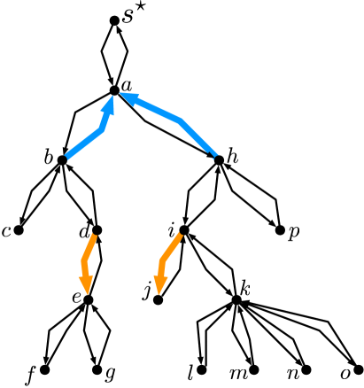
Figure 11: An illustration of an LCA$(e,j)$ query. We do a RangeMin query on the interval $e_{0}=(d,e),\ldots,(i,j)=e_{1}$ and retrieve the edge $\hat{e}=e_{e}=(b,g)$ with weight $\operatorname{depth}_{T}(g)$. We then find $\tilde{e}=(g,s^{\star})$ and its predecessor $\tilde{e}^{\prime}=(h,g)$. Another RangeMin query on the interval $(i,j),\ldots,(h,g)$ returns $e_{j}=(h,g)$.

We have reduced our dynamic tree problem to a dynamic weighted list problem. We now explain how the dynamic list problem can be solved with balanced trees.

Fix a parameter $\kappa\geq 1$ and let $n$ be the total number of elements in all lists. We now argue that Split, Concatenate, and Add can be implemented in $O(\kappa n^{1/\kappa})$ time and Weight and RangeMin take $O(\kappa)$ time. We store the elements of each list $L$ at the leaves of a rooted tree $\mathcal{T}(L)$. It satisfies the following invariants.

1. Each node $\gamma$ of $\mathcal{T}(L)$ stores a weight offset $w(\gamma)$, a min-weight value $\min(\gamma)$ and a pointer $\operatorname{ptr}(\gamma)$. The weight of (leaf) $e\in L$ is the sum of the $w(\cdot)$-values of its ancestors, including $e$. The sum of $\min(\gamma)$ and the $w(\cdot)$-values of all strict ancestors of $\gamma$ is exactly the weight of the minimum weight descendant of $\gamma$, and $\operatorname{ptr}(\gamma)$ points to this element.

2. Non-root internal nodes have between $n^{1/\kappa}$ and $3n^{1/\kappa}$ children. In particular, the tree has height at most $\kappa$.

3. Each internal node $\gamma$ maintains an $O(1)$-time range minimum structure [4] over the vector of $\min(\cdot)$-values of its children.

It is easy to show that Split and Concatenate can be implemented to satisfy Invariant II by destroying/rebuilding $O(1)$ nodes at each level of $\mathcal{T}$. Each costs $O(n^{1/\kappa})$ time to update the information covered by Invariants I and III. The total time is therefore $O(\kappa n^{1/\kappa})$. By Invariant I, a Weight$(e_{0})$ query takes $O(\kappa)$ time to sum all of $e_{0}$’s ancestors’ $w(\cdot)$-values. Consider an Add$(e_{0},e_{1},\delta)$ or RangeMin$(e_{0},e_{1})$ operation. By Invariant II, the interval $(e_{0},\ldots,e_{1})$ is covered by $O(\kappa n^{1/\kappa})$ $\mathcal{T}$-nodes, and furthermore, those nodes can be arranged into less than $2\kappa$ contiguous intervals of siblings. Thus, an Add$(e_{0},e_{1})$ can be implemented in $O(\kappa n^{1/\kappa})$ time by adding $\delta$ to the $w(\cdot)$-values of these nodes and rebuilding the affected range-min structures from Invariant III. A RangeMin is reduced to $O(\kappa)$ range-minimum queries (from Invariant III) and adjusting the answers by the $w(\cdot)$-values of their ancestors (Invariant I). Each range-min query takes $O(1)$ time and there are $O(\kappa)$ ancestors with relevant $w(\cdot)$-values. Thus RangeMin takes $O(\kappa)$ time.

We have shown that the dynamic tree operations necessary for an MSSP structure can be implemented with a flexible tradeoff between update time and query time. Moreover, this lower bound meets the Pǎtraşcu-Demaine lower bound [34]. We leave it as an open problem to implement the full complement of operations supported by Link-Cut trees, with update time $O(\kappa n^{1/\kappa})$ and query time $O(\kappa)$.

Appendix B Multiple Holes and Nonsimple Cycles

We have assumed for simplicity that all regions are bounded by a simple cycle, and therefore have a single hole. We now show how these assumptions can be removed.

Let us first illustrate how a region $R$ may get a hole with a non-simple boundary cycle. The hierarchical decomposition algorithm of Klein, Mozes, and Sommer [29] produces a binary decomposition tree, of which our $\vec{r}$-decomposition is a coarsening. It proceeds by finding a separating cycle (as in Miller [31]), and recursively decomposes the graph inside the cycle and outside the cycle. At intermediate stages the working graph contains several holes, but Miller’s theorem [31] only guarantees that a small cycle separator exists if the graph is triangulated. To that end, the decomposition [29] puts an artificial vertex inside each hole and triangulates the hole. See Figure 12(a,b). If the cycle separator $C$ (blue cycle in Figure 12(b)) includes a hole-vertex $v$, we splice out $v$ and replace it with an interval of the boundary of the hole. If $C$ also includes edges on the boundary of the hole (Figure 12(c)), the modified cycle may not be simple. If this is the case, we “cut” along non-simple parts of the cycle, replicating all such vertices and their incident cycle edges. We then join pairs of identical vertices with zero-length edges (pink edges in Figure 12(c)), and triangulate with large-length edges. This transformation clearly preserves planarity and does not change the underlying metric.

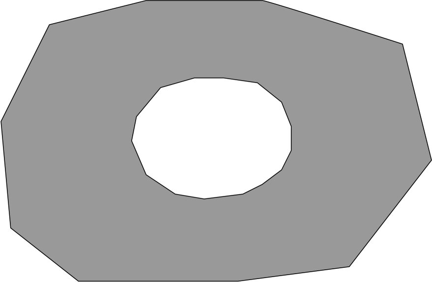
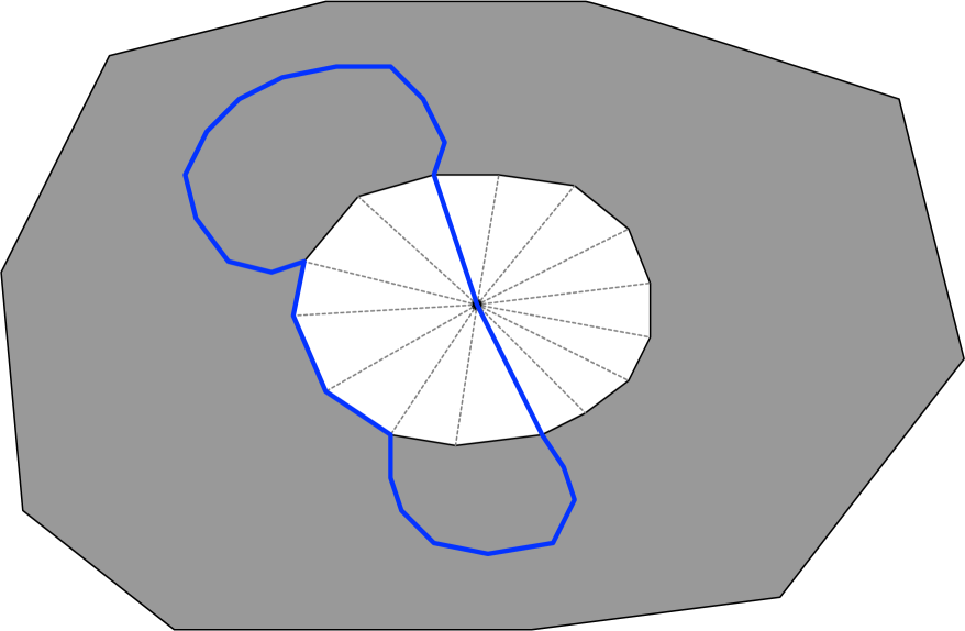
(a)	(b)
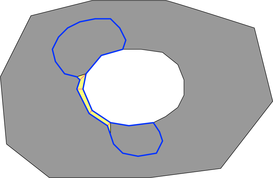
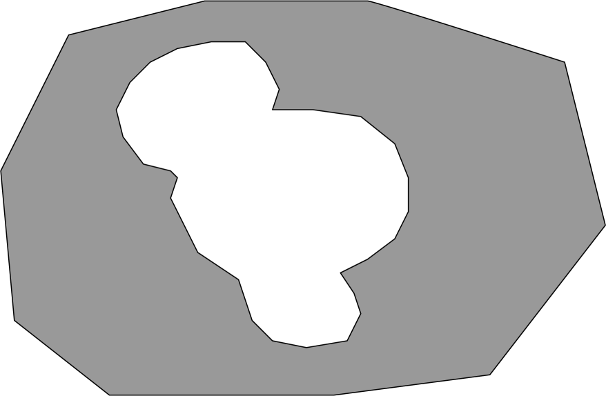
(c)	(d)

Figure 12: (a) A subgraph with two holes. (b) We put a vertex in each hole and triangulate the hole. (The triangulation of the exterior hole is not drawn, for clarity.) A simple cycle sparator (blue curve) is found in this graph. (c) The cycle is mapped to a possibly non-simple cycle in the original graph that avoids hole-vertices. We cut along non-simple parts of the cycle, duplicating the vertices and their adjacent edges on the cycle. (d) The graph remaining after removing the subgraph enclosed by the cycle from (c).

Turning to the issue of multiple holes, we first make some observations about their structural organization. Fix any hole $g$ of region $R_{i+1}$ and let $R_{i}$ be a child of $R_{i+1}$. There is a unique hole $\operatorname{par}_{R_{i}}(g)$ in $R_{i}$ such that $g$ lies in $R_{i}^{\operatorname{par}_{R_{i}}(g),\operatorname{out}}$, which we refer to as the parent of $g$ in $R_{i}$. (Note that the ancestry of holes goes in the opposite direction of the ancestry of regions in the $\vec{r}$-decomposition.) In a distance query we only deal with a series of regions $R_{0}=\{u\},R_{1},\ldots,R_{m}=G$. The holes of these regions form a hierarchy, rooted at $\{u\}$, which we view as a degenerate hole. For notational simplicity we use “$g$” to refer to the set of vertices on hole $g$.

Lemma B.1.

(See [9, §4.3.2]) There is an $\tilde{O}(n)$-space data structure that, given $u,v$ can report in $O(m)$ time the regions $R_{0}=\{u\},R_{1},\cdots,R_{t+1}$ and holes $h_{0},h_{1},\ldots,h_{t}$ such that $v\in R_{i}^{h_{i},\operatorname{out}}$, $v\not\in R_{t}$, and $v\in R_{t+1}$.

The method of [9] simply involves doing a least common ancestor query of $\{u\}$ and $\{v\}$ in the “full” binary decomposition returned by the [29] algorithm (from which our $\vec{r}$-decomposition is a coarsening) in order to retrieve $h_{t}$. The holes $h_{t-1},\ldots,h_{0}$ can then be found by following parent pointers in $O(m)$ time.

B.1 Data Structures

The following modifications are made to parts (A)–(E) of the data structure. In all cases the space usage is unchanged, asymptotically.

1. (MSSP Structures) For each $i\in[0,m-1]$, each $R_{i}\in\mathcal{R}_{i}$ with parent $R_{i+1}$ and each hole $h_{i}$ of $R_{i}$, we build a MSSP structure for $R_{i}^{h_{i},\operatorname{out}}$ that answers distance queries and LCA queries w.r.t. $R_{i}^{h_{i},\operatorname{out}}$ for vertices in $R_{i}^{h_{i},\operatorname{out}}\cap R_{i+1}$.

2. (Voronoi Diagrams) For each $i\in[0,m-1]$, each $R_{i}\in\mathcal{R}_{i}$ with parent $R_{i+1}\in\mathcal{R}_{i+1}$, each hole $h_{i+1}$ of $R_{i+1}$ with parent $h_{i}=\operatorname{par}_{R_{i}}(h_{i+1})$, and each $q\in h_{i}$, we store the dual representation of Voronoi diagram $\mathrm{VD}^{*}_{\operatorname{out}}(q,R_{i+1},h_{i+1})$ defined to be $\mathrm{VD}^{*}[R_{i+1}^{h_{i+1},\operatorname{out}},h_{i+1},\omega]$ with $\omega(s)=\operatorname{dist}_{G}(q,s)$.

3. (More Voronoi Diagrams) For each $i\in[1,m-1]$, each $R_{i}\in\mathcal{R}_{i}$, each hole $h_{i}$ of $R_{i}$, and each $q\in h_{i}$, we store $\mathrm{VD}^{*}_{\operatorname{out}}(q,R_{i},h_{i})$, which is $\mathrm{VD}^{*}[R_{i}^{h_{i},\operatorname{out}},h_{i},\omega]$ with $\omega(s)=\operatorname{dist}_{G}(q,s)$.

4. (Chord Trees; Piece Trees) For each $i\in[1,m-1]$, each $R_{i}\in\mathcal{R}_{i}$, each hole $h_{i}$ of $R_{i}$, and source $q\in h_{i}$, we store a chord tree $T_{q}^{R_{i},h_{i}}$ obtained by restricting the SSSP tree with source $q$ to $h_{i}$. An edge in $T_{q}^{R_{i},h_{i}}$ is designated a chord if the corresponding path lies in $R_{i}^{h_{i},\operatorname{out}}$ and is internally vertex disjoint from $h_{i}$. $\mathcal{C}_{q}^{R_{i},h_{i}},\mathcal{P}_{q}^{R_{i},h_{i}},\mathcal{T}_{q}^{R_{i},h_{i}}$ are defined analogously, and data structures are built to answer $\boldsymbol{\mathsf{MaximalChord}}$ and $\boldsymbol{\mathsf{AdjacentPiece}}$ with respect to $q,R_{i},h_{i}$.

5. (Site Tables; Side Tables) Fix an $i$ and a Voronoi diagram $\mathrm{VD}^{*}_{\operatorname{out}}=\mathrm{VD}^{*}_{\operatorname{out}}(u^{\prime},R_{i},h_{i})$ from part (B) or (C). Let $f^{*}$ be any node in the centroid decomposition of $\mathrm{VD}^{*}_{\operatorname{out}}$ with $y_{j},s_{j}$ defined as usual, $j\in\{0,1,2\}$. Let $R_{i^{\prime}}\in\mathcal{R}_{i^{\prime}}$ be an ancestor of $R_{i}$, $i^{\prime}>i$, and $h_{i^{\prime}}$ be a hole of $R_{i^{\prime}}$ lying in $R_{i}^{h_{i},\operatorname{out}}$. We store the first and last vertices $q,x$ on the shortest $s_{j}$-$y_{j}$ path that lie on $h_{i^{\prime}}$, as well as $\operatorname{dist}_{G}(u^{\prime},x)$.

   We also store whether $R_{i^{\prime}}^{h_{i^{\prime}},\operatorname{out}}$ lies to the left or right of the site-centroid-site chord $\overrightarrow{s_{j}y_{j}y_{j-1}s_{j-1}}$, or Null if the relationship cannot be determined.

B.2 Query

At the first call to $\boldsymbol{\mathsf{Dist}}(u,v,R_{0})$ we apply Lemma B.1 to generate the regions $R_{1},\ldots,R_{t+1}$ and holes $h_{1},\ldots,h_{t}$ that will be accessed in all recursive calls, in $O(m)$ time.

The shortest $u$-$v$ path in $G$ will eventually cross $h_{1},\ldots,h_{t}$. The vertex $u_{i}$ is now defined to be the last vertex in $h_{i}$ on the shortest $u$-$v$ path. Given $u_{i}$, we find $u_{i+1}$ by solving a point location problem in $\mathrm{VD}^{*}_{\operatorname{out}}(u_{i},R_{i+1},h_{i+1})$. The $\boldsymbol{\mathsf{Navigation}}$ routine focuses on the subgraph $R_{t}^{h_{t},\operatorname{out}}$ rather than $R_{t}^{\operatorname{out}}$. The general problem is no different than the single hole case, except that there may be $O(1)$ holes of $R_{t+1}$ lying in $R_{t}^{h_{t},\operatorname{out}}$, which does not cause further complications.

Appendix C Construction

As in [9], we use dense distance graphs as a tool to build our oracle. To simplify the description, we still assume that $\partial R$ lies on a single simple cycle for every region $R$ in the $\vec{r}$-division. Generalizing to multiple holes and nonsimple cycles is straightforward.

The dense distance graph of a region $R$ (denoted by $\mathsf{DDG}[R]$) is a complete directed graph on the vertices of $\partial R$, in which the length of $(u,v)$ is $\operatorname{dist}_{R}(u,v)$. We say that this kind of DDGs are internal and, similarly, define the external DDG of a region $R$ (denoted by $\mathsf{DDG}[R^{\operatorname{out}}]$) as a complete directed graph on $\partial R$, in which the length of $(u,v)$ is $\operatorname{dist}_{R^{\operatorname{out}}}(u,v)$.

The FR-Dijkstra algorithm [18] is an efficient implementation of Dijkstra’s algorithm [14] on DDGs. In particular, it simulates the behavior of the heap in Dijkstra’s algorithm without explicitly scanning every edge in the DDGs. In fact, the FR-Dijkstra algorithm can run on a union of DDGs [18]. Moreover, it is shown in [6] that it can also run compatibly with a traditional Dijkstra algorithm. Suppose we have a graph $H$ that consists of a subgraph of $G$ on $n_{0}$ vertices, and $k$ DDGs on $n_{1},n_{2},\ldots,n_{k}$ vertices. The FR-Dijkstra algorithm can be implemented on $H$ in $\tilde{O}(N)$ time, where $N=\sum_{i}n_{i}$.

Before the construction of DDGs and our oracle, we first prepare Klein’s MSSP structures (part (F) below). Note that MSSP structures in part (F) are only used in the constructions of DDGs and part (E). They are not stored in our oracle and unrelated to the MSSP structures from part (A).

1. (More MSSP Structures) For each $i\in[0,m-1]$, each $R_{i}\in\mathcal{R}_{i}$ with parent $R_{i+1}\in\mathcal{R}_{i+1}$, we build two MSSP structures for $R_{i}^{\operatorname{out}}\cap R_{i+1}$ with sources on $\partial R_{i}$ and $\partial R_{i+1}$, respectively, and an MSSP structure for $R_{i}$ with sources on $\partial R_{i}$.

   All these MSSP structures are constructed using Klein’s MSSP algorithm [28] or the one in Appendix A (with $\kappa=\log n$) in $\tilde{O}(\sum_{i}\frac{n}{r_{i}}r_{i+1})=\tilde{O}(mn^{1+1/m})$ time.

We then compute, for each region $R_{i}$ in the $\vec{r}$-division, the internal DDG, the external DDG, and the DDG of $R_{i}^{\operatorname{out}}\cap R_{i+1}$ (denoted by $\mathsf{DDG}[R_{i}^{\operatorname{out}}\cap R_{i+1}]$) defined as the complete graph with vertices $\partial R_{i}$ and $\partial R_{i+1}$ and edge weights the distances in $R_{i}^{\operatorname{out}}\cap R_{i+1}$. The internal DDG and $\mathsf{DDG}[R_{i}^{\operatorname{out}}\cap R_{i+1}]$ for each region $R_{i}$ can be computed using MSSP structures in part (F) in $\tilde{O}(r_{i})$ and $\tilde{O}(r_{i+1})$ time respectively, so it takes $\tilde{O}(\sum_{i}\frac{n}{r_{i}}(r_{i}+r_{i+1}))=\tilde{O}(mn^{1+1/m})$ time over all regions. To compute the external DDGs, we consider a top-down process on the $\vec{r}$-division. The external DDG for $R_{i}$ can be computed by running the FR-Dijkstra algorithm sourced from $\partial R_{i}$ on the union of $\mathsf{DDG}[R_{i+1}^{\operatorname{out}}]$ and $\mathsf{DDG}[R_{i}^{\operatorname{out}}\cap R_{i+1}]$. The size of the union is $O(\sqrt{r_{i+1}})$, so computing $\mathsf{DDG}[R_{i}^{\operatorname{out}}]$ takes $\tilde{O}(\sqrt{r_{i}r_{i+1}})$ time, and the construction time over all external DDGs is $\tilde{O}(\sum_{i}\frac{n}{r_{i}}\sqrt{r_{i}r_{i+1}})=\tilde{O}(mn^{1+1/(2m)})$. The total construct time for all DDGs is $\tilde{O}(mn^{1+1/m})$.

With dense distance graphs, all components in the oracle can be constructed as follows.

1. MSSP Structures

   Recall that our MSSP structure for $R_{i}^{\operatorname{out}}$ with sites $\partial R_{i}$ is obtained by contracting subpaths in $R_{i+1}^{\operatorname{out}}$ of the SSSP trees into single edges. In order to build the MSSP structure using dynamic trees, it suffices to compute the contracted shortest path tree for every source on $\partial R_{i}$ and then compare the differences between the trees of two adjacent sources on $\partial R_{i}$.

   For a single source on $\partial R_{i}$, the contracted shortest path tree can be computed with FR-Dijkstra algorithm on the union of subgraph $R_{i}^{\operatorname{out}}\cap R_{i+1}$ and $\mathsf{DDG}[R_{i+1}^{\operatorname{out}}]$ in time $\tilde{O}(r_{i+1})$. Thus, the time for constructing and comparing the shortest path trees is $\tilde{O}(r_{i+1}\sqrt{r_{i}})$. After that, an MSSP structure for $R_{i}^{\operatorname{out}}$ can be built in time $\tilde{O}((r_{i+1}+\sqrt{r_{i}r_{i+1}})\kappa n^{1/\kappa})$. The total time to construct all MSSP structures is $\tilde{O}(\sum_{i}\frac{n}{r_{i}}(r_{i+1}\sqrt{r_{i}}+r_{i+1}\kappa n^{1/\kappa}))=\tilde{O}(n^{3/2+1/m}m+n^{1+1/\kappa+1/m}m\kappa)$.

   Remark 2.

   Notice that in our MSSP structures for $R_{i}^{\operatorname{out}}$, a contracted subpath should be “strictly” inside $R_{i+1}^{\operatorname{out}}$, which contains no vertices belonging to $R_{i}^{\operatorname{out}}\cap R_{i+1}$ except its endpoints. However, the underlying shortest paths represented by edges in $\mathsf{DDG}[R_{i+1}^{\operatorname{out}}]$ may not satisfy this condition. To fix this problem, we add small perturbation to all edge weights in DDGs. Note that this will not break the Monge property of a DDG’s adjacency matrix, on which the FR-Dijkstra algorithm relies. In fact, all different shortest paths from the source to $v$ in the union represent the same unique underlying shortest path in $R_{i}^{\operatorname{out}}$, and we choose the one passing as many as possible vertices in the union, on which each edge of the DDG is “strictly” inside $R_{i+1}^{\operatorname{out}}$. This mechanism will also be used below.

2. Voronoi Diagrams

   The additive weights of all Voronoi diagrams can be computed by a FR-Dijkstra algorithm running on a union of proper DDGs. Specific to $\mathrm{VD}^{*}_{\operatorname{out}}(u_{i},R_{i+1})$ in (B), additive weights are given by considering the union of $\mathsf{DDG}[R_{i}],\mathsf{DDG}[R_{i}^{\operatorname{out}}\cap R_{i+1}],\mathsf{DDG}[R_{i+1}^{\operatorname{out}}]$ in $\tilde{O}(\sqrt{r_{i+1}})$ time. For $\mathrm{VD}^{*}_{\operatorname{out}}(u_{i},R_{i})$ in (C), we focus on the union of $\mathsf{DDG}[R_{i}],\mathsf{DDG}[R_{i}^{\operatorname{out}}]$ and additive weights can be computed in time $\tilde{O}(\sqrt{r_{i}})$. The overall time to compute additive weights is $\tilde{O}(\sum_{i}\frac{n}{r_{i}}\sqrt{r_{i}}\sqrt{r_{i+1}})=\tilde{O}(mn^{1+1/(2m)})$.

   An efficient algorithm to compute the dual representation of a Voronoi diagram is presented in [9], by considering the complete recursive decomposition of $G$. Note that the complete recursive decomposition of $G$ is a binary decomposition tree, and the $\vec{r}$-division is a coarse version of it. It can be obtained in $O(n)$ time [29].

   Lemma C.1.

   (Cf. Charalampopoulos et al. [9], Theorem 12) Given a complete recursive decomposition of $G$, in which every region has been preprocessed for the FR-Dijkstra algorithm as in [18], the dual representation of Voronoi diagrams on the complement of a specific region $R$ with sites $\partial R$ and arbitrary input additive weights can be computed in time $\tilde{O}(\sqrt{|G|\cdot|\partial R|})$.

   By Lemma C.1, the total construction time for the dual representations is

   $$\tilde{O}\left(\sum_{i}\frac{n}{r_{i}}\sqrt{r_{i}}\sqrt{n\sqrt{r_{i+1}}}+\sum_{i}\frac{n}{r_{i}}\sqrt{r_{i}}\sqrt{n\sqrt{r_{i}}}\right)=\tilde{O}\left(n^{3/2+1/(4m)}\right),$$

   which is also the construction time for parts (B) and (C).

3. Chord Trees and Piece Trees

   Recall that the chord tree $T_{q}^{R_{i}}$ is obtained from the shortest path tree in $G$ sourced from $q\in\partial R_{i}$ by contracting all paths between vertices in $\partial R_{i}$ into single edges. Thus, it can be computed by running FR-Dijkstra on the union of $\mathsf{DDG}[R_{i}]$ and $\mathsf{DDG}[R_{i}^{\operatorname{out}}]$ in $\tilde{O}(\sqrt{r_{i}})$ time.

   Regarding the construction of piece tree $\mathcal{T}_{q}^{R_{i}}$, we first extract all the chords on $T_{q}^{R_{i}}$ in $R_{i}^{\operatorname{out}}$, i.e. the chord set $\mathcal{C}_{q}^{R_{i}}$. We treat each chord in $\mathcal{C}_{q}^{R_{i}}$ as an undirected edge and consider the undirected planar graph $Q$ which is the union of $\mathcal{C}_{q}^{R_{i}}$ and $\partial R$. Observe that each piece in $\mathcal{P}_{q}^{R_{i}}$ relates to a face of $Q$. The piece tree $\mathcal{T}_{q}^{R_{i}}$ can be built straightforwardly in time $\tilde{O}(\sqrt{r_{i}})$. With the graph $Q$ and the piece tree $\mathcal{T}_{q}^{R_{i}}$, the data structure supporting $\boldsymbol{\mathsf{MaximalChord}}$ and $\boldsymbol{\mathsf{AdjacentPiece}}$ in Lemma 4.2 can also be constructed in time $\tilde{O}(\sqrt{r_{i}})$ for the given $q,R_{i}$.

   The total time for the whole part (D) is $\tilde{O}(\sum_{i}\frac{n}{r_{i}}\sqrt{r_{i}}\sqrt{r_{i}})=\tilde{O}(nm)$.

4. Site Tables and Side Tables

   We focus on the site table and side table for a specific $\mathrm{VD}^{*}_{\operatorname{out}}(u,R_{i})$, and do some preparations.

   • Observe that the union of

     $$\mathsf{DDG}[R_{i}^{\operatorname{out}}\cap R_{i+1}],\mathsf{DDG}[R_{i+1}^{\operatorname{out}}\cap R_{i+2}],\ldots,\mathsf{DDG}[R_{m-1}^{\operatorname{out}}]$$

     contains exactly all boundary vertices in $R_{i}^{\operatorname{out}}$ of ancestors $R_{i},R_{i+1},\ldots,R_{m-1}$. We use $H$ to denote this union with an artificial super-source $u^{\prime}$ connected to each site $s\in\partial R_{i}$ with weight $\omega(s)$, and construct the shortest path tree $T_{H}$ in $H$ sourced from the super-source $u^{\prime}$ by FR-Dijkstra algorithm, which costs $\tilde{O}(\sqrt{n})$ time.

   Remember that the site table stores the first and last vertices of each site-centroid $s$-$y$ path on the boundary of each ancestor $R_{i^{\prime}}$ ($i^{\prime}\geq i$). We first find the last vertex $x$ on the $s$-$y$ path belonging to $H$. Assume that $y\in R_{k+1}$ but $y\notin R_{k}$, where $R_{k},R_{k+1}$ are ancestors of $R_{i}$. We can observe that $x$ is the vertex in $\partial R_{k}\cup\partial R_{k+1}$ with the minimal $\operatorname{dist}_{H}(u^{\prime},x)+\operatorname{dist}_{R_{k}^{\operatorname{out}}\cap R_{k+1}}(x,v)$ (breaking ties in favor of larger $\operatorname{dist}_{H}(u^{\prime},x)$). The former is given by $T_{H}$ and the latter can be found by querying MSSP structures in (F) for $R_{k}^{\operatorname{out}}\cap R_{k+1}$. The calculation of $x$ needs time $\tilde{O}(|\partial R_{k+1}|)=\tilde{O}(\sqrt{n})$. Observe that the $u^{\prime}$-$x$ path on $T_{H}$ includes all boundary vertices of upper regions on the $s$-$y$ path. By retrieving the $u^{\prime}$-to-$x$ path on $T_{H}$ in $O(\sqrt{n})$ time, we can get the required information for the site table. The construction time of a site table for $\mathrm{VD}^{*}_{\operatorname{out}}(u,R_{i})$ is $\tilde{O}(\sqrt{r_{i}}\sqrt{n})$.

   In the side table, we will store the relationship (left/right/Null) between each site-centroid-site chord $C=\overrightarrow{s_{j}y_{j}y_{j-1}s_{j-1}}$ (using the notations in Figure 3) and each ancestor $R_{i^{\prime}}^{\operatorname{out}}$ $(i^{\prime}\geq i)$. With the technique used in the construction of site tables, we can extract all vertices of $C$ on each $\partial R_{i^{\prime}}$ from $T_{H}$, and then determine the relationship between $C$ and each $R_{i^{\prime}}^{\operatorname{out}}$ with boundary vertices on $C$. For each $R_{i^{\prime}}^{\operatorname{out}}$ that $C$ contains no vertices on $\partial R_{i^{\prime}}$, we pick an arbitrary vertex $z$ on $\partial R_{i^{\prime}}$. We can retrieve from $T_{H}$ the $u^{\prime}$-$z$ path and find the site $s_{z}$ s.t. $z\in\operatorname{Vor}(s_{z})$. This can be done in $O(\sqrt{n})$ time. With $T_{H}$ and MSSP structures in part (F), we can determine the pairwise relationships among $s_{j}$-$y_{j}$, $s_{j-1}$-$y_{j-1}$ and $s_{z}$-$z$ shortest paths and know whether $z$ lies to the left or right of $C$, which immediately shows the relationship between $C$ and $R_{i^{\prime}}^{\operatorname{out}}$. The construction time for a side table of $\mathrm{VD}^{*}_{\operatorname{out}}(u,R_{i})$ is $\tilde{O}(\sqrt{r_{i}}m\sqrt{n})$.

   The total time for building all site tables and side tables is $\tilde{O}(\sum_{i}\frac{n}{r_{i}}\sqrt{r_{i}}\sqrt{r_{i+1}}m\sqrt{n})=\tilde{O}(n^{3/2+1/(2m)}m^{2})$.

The overall construction time is $\tilde{O}(n^{3/2+1/m}+n^{1+1/m+1/\kappa})$ since $m$ and $\kappa$ should be functions of $n$ that are $O(\log n)$.

References

- [1] Ittai Abraham and Cyril Gavoille. On approximate distance labels and routing schemes with affine stretch. In Proceedings of the 25th International Symposium on Distributed Computing (DISC), volume 6950 of Lecture Notes in Computer Science, pages 404–415, 2011.
- [2] Rachit Agarwal. The space-stretch-time tradeoff in distance oracles. In Proceedings of the 22nd European Symposium on Algorithms (ESA), volume 8737 of Lecture Notes in Computer Science, pages 49–60, 2014.
- [3] Srinivasa Rao Arikati, Danny Z. Chen, L. Paul Chew, Gautam Das, Michiel H. M. Smid, and Christos D. Zaroliagis. Planar spanners and approximate shortest path queries among obstacles in the plane. In Proceedings 4th Annual European Symposium on Algorithms (ESA), volume 1136 of Lecture Notes in Computer Science, pages 514–528, 1996.
- [4] Michael A. Bender and Martin Farach-Colton. The LCA problem revisited. In Proceedings of the 4th Latin American Symposium on Theoretical Informatics (LATIN), volume 1776 of Lecture Notes in Computer Science, pages 88–94. Springer, 2000.
- [5] Michael A. Bender and Martin Farach-Colton. The level ancestor problem simplified. Theor. Comput. Sci., 321(1):5–12, 2004.
- [6] Glencora Borradaile, Piotr Sankowski, and Christian Wulff-Nilsen. Min -cut oracle for planar graphs with near-linear preprocessing time. ACM Transactions on Algorithms, 11(3):1–29, 2015.
- [7] Sergio Cabello. Many distances in planar graphs. Algorithmica, 62(1-2):361–381, 2012.
- [8] Sergio Cabello. Subquadratic algorithms for the diameter and the sum of pairwise distances in planar graphs. ACM Trans. Algorithms, 15(2):21:1–21:38, 2019.
- [9] Panagiotis Charalampopoulos, Paweł Gawrychowski, Shay Mozes, and Oren Weimann. Almost optimal distance oracles for planar graphs. In Proceedings of the 51st Annual ACM Symposium on Theory of Computing (STOC), pages 138–151, 2019.
- [10] Danny Z. Chen and Jinhui Xu. Shortest path queries in planar graphs. In Proceedings of the 32nd Annual ACM Symposium on Theory of Computing (STOC), pages 469–478, 2000.
- [11] Vincent Cohen-Addad, Søren Dahlgaard, and Christian Wulff-Nilsen. Fast and compact exact distance oracle for planar graphs. In Proceedings 58th Annual IEEE Symposium on Foundations of Computer Science (FOCS), pages 962–973, 2017.
- [12] Paul F. Dietz. Fully persistent arrays. In Proceedings of the First Workshop on Algorithms and Data Structures (WADS), volume 382 of Lecture Notes in Computer Science, pages 67–74, 1989.
- [13] Martin Dietzfelbinger, Anna R. Karlin, Kurt Mehlhorn, Friedhelm Meyer auf der Heide, Hans Rohnert, and Robert Endre Tarjan. Dynamic perfect hashing: Upper and lower bounds. In Proceedings of the 29th Annual IEEE Symposium on Foundations of Computer Science (FOCS), pages 524–531, 1988.
- [14] Edsger W Dijkstra. A note on two problems in connexion with graphs. Numerische mathematik, 1(1):269–271, 1959.
- [15] Hristo Djidjev. On-line algorithms for shortest path problems on planar digraphs. In Proceedings of the 22nd International Workshop on Graph-Theoretic Concepts in Computer Science (WG), volume 1197 of Lecture Notes in Computer Science, pages 151–165, 1996.
- [16] James R. Driscoll, Neil Sarnak, Daniel Dominic Sleator, and Robert Endre Tarjan. Making data structures persistent. J. Comput. Syst. Sci., 38(1):86–124, 1989.
- [17] Jeff Erickson, Kyle Fox, and Luvsandondov Lkhamsuren. Holiest minimum-cost paths and flows in surface graphs. In Proceedings of the 50th Annual ACM Symposium on Theory of Computing (STOC), pages 1319–1332, 2018.
- [18] Jittat Fakcharoenphol and Satish Rao. Planar graphs, negative weight edges, shortest paths, and near linear time. J. Comput. Syst. Sci., 72(5):868–889, 2006.
- [19] Greg N. Frederickson. Fast algorithms for shortest paths in planar graphs, with applications. SIAM J. Comput., 16(6):1004–1022, 1987.
- [20] Pawel Gawrychowski, Shay Mozes, Oren Weimann, and Christian Wulff-Nilsen. Better tradeoffs for exact distance oracles in planar graphs. In Proceedings of the 29th Annual ACM-SIAM Symposium on Discrete Algorithms (SODA), pages 515–529, 2018.
- [21] Torben Hagerup. Still simpler static level ancestors. CoRR, abs/2005.11188, 2020.
- [22] Dov Harel and Robert Endre Tarjan. Fast algorithms for finding nearest common ancestors. SIAM J. Comput., 13(2):338–355, 1984.
- [23] Monika Rauch Henzinger and Valerie King. Randomized fully dynamic graph algorithms with polylogarithmic time per operation. J. ACM, 46(4):502–516, 1999.
- [24] Donald B. Johnson. Efficient algorithms for shortest paths in sparse networks. J. ACM, 24(1):1–13, 1977.
- [25] Ken-ichi Kawarabayashi, Philip N. Klein, and Christian Sommer. Linear-space approximate distance oracles for planar, bounded-genus and minor-free graphs. In Proceedings of the 38th Int’l Colloquium on Automata, Languages and Programming (ICALP), volume 6755 of Lecture Notes in Computer Science, pages 135–146, 2011.
- [26] Ken-ichi Kawarabayashi, Christian Sommer, and Mikkel Thorup. More compact oracles for approximate distances in undirected planar graphs. In Proceedings of the 24th ACM-SIAM Symposium on Discrete Algorithms (SODA), pages 550–563, 2013.
- [27] Philip Klein. Preprocessing an undirected planar network to enable fast approximate distance queries. In Proceedings of the 13th ACM-SIAM Symposium on Discrete Algorithms (SODA), pages 820–827, 2002.
- [28] Philip N. Klein. Multiple-source shortest paths in planar graphs. In Proceedings of the 16th Annual ACM-SIAM Symposium on Discrete Algorithms (SODA), pages 146–155, 2005.
- [29] Philip N. Klein, Shay Mozes, and Christian Sommer. Structured recursive separator decompositions for planar graphs in linear time. In Proceedings of the 45th Annual ACM Symposium on Theory of Computing (STOC), pages 505–514, 2013.
- [30] Richard J. Lipton and Robert Endre Tarjan. Applications of a planar separator theorem. SIAM J. Comput., 9(3):615–627, 1980.
- [31] Gary L. Miller. Finding small simple cycle separators for 2-connected planar graphs. J. Comput. Syst. Sci., 32(3):265–279, 1986.
- [32] Shay Mozes and Christian Sommer. Exact distance oracles for planar graphs. In Proceedings of the 23rd ACM-SIAM Symposium on Discrete Algorithms (SODA), pages 209–222, 2012.
- [33] Yahav Nussbaum. Improved distance queries in planar graphs. In Proceedings 12th Int’l Workshop on Algorithms and Data Structures (WADS), pages 642–653, 2011.
- [34] Mihai Patrascu and Erik D. Demaine. Logarithmic lower bounds in the cell-probe model. SIAM J. Comput., 35(4):932–963, 2006.
- [35] Mihai Patrascu and Liam Roditty. Distance oracles beyond the Thorup-Zwick bound. SIAM J. Comput., 43(1):300–311, 2014.
- [36] Neil Sarnak and Robert Endre Tarjan. Planar point location using persistent search trees. Commun. ACM, 29(7):669–679, 1986.
- [37] Daniel Dominic Sleator and Robert Endre Tarjan. A data structure for dynamic trees. J. Comput. Syst. Sci., 26(3):362–391, 1983.
- [38] Christian Sommer. Shortest-path queries in static networks. ACM Computing Surveys, 46(4):1–31, 2014.
- [39] Christian Sommer, Elad Verbin, and Wei Yu. Distance oracles for sparse graphs. In Proceedings of the 50th IEEE Symposium on Foundations of Computer Science (FOCS), pages 703–712, 2009.
- [40] Mikkel Thorup. Compact oracles for reachability and approximate distances in planar digraphs. J. ACM, 51(6):993–1024, 2004.
- [41] Mikkel Thorup and Uri Zwick. Approximate distance oracles. J. ACM, 52(1):1–24, 2005.
- [42] Christian Wulff-Nilsen. Algorithms for planar graphs and graphs in metric spaces. PhD thesis, PhD thesis, University of Copenhagen, 2010.