Speiser class Julia sets with dimension near one

Abstract.

For any $\delta>0$ we construct an entire function $f$ with three singular values whose Julia set has Hausdorff dimension at most $1+\delta$. Stallard proved that the dimension must be strictly larger than $1$ whenever $f$ has a bounded singular set, but no examples with finite singular set and dimension strictly less than $2$ were previously known.

1. Introduction

Suppose $f$ is an entire function. The Fatou set $\mathcal{F}(f)$ is the union of all open disks on which the iterates $f,f^{2},f^{3},\dots$ form a normal family and the Julia set $\mathcal{J}(f)$ is the complement of this set. In 1975 Baker [2] proved that if $f$ is transcendental (i.e., not a polynomial), then the Fatou set has no unbounded, multiply connected components. This implies the Julia set contains a non-trivial continuum and hence has Hausdorff dimension at least $1$, but it is difficult to build examples that come close to attaining this minimum; constructing such examples is the transcendental counterpart of finding polynomial Julia sets with dimension near 2 (e.g., [16], [36], [43]). For transcendental entire functions, finding “large” Julia sets is easier: Misiurewicz [29] proved that the Julia set of $f(z)=\exp(z)$ is the whole plane, and McMullen [27] gave explicit families where the Julia set is not the whole plane, but still has dimension $2$ (even positive area). Stallard [37], [38] proved that the Hausdorff dimension of a transcendental Julia set can attain every value in the interval $(1,2]$, and the second author [14] recently constructed a transcendental Julia set with dimension $1$, Baker’s lower bound.

The singular set of an entire function $f$ is the closure of its critical values and finite asymptotic values (limits of $f$ along a curve to $\infty$) and will be denoted $S(f)$. The Eremenko-Lyubich class $\mathcal{B}$ consists of functions such that $S(f)$ is a bounded set (such functions are also called bounded-type). The Speiser class $\mathcal{S}\subset\mathcal{B}$ consists of those functions for which $S(f)$ is a finite set. These are important classes in transcendental dynamics and it is an interesting problem to understand their differences and similarities. For example, functions in $\mathcal{S}$ can’t have wandering domains, whereas those in $\mathcal{B}$ can, [11], [18], [22]. Stallard’s examples with $1<\dim(\mathcal{J})<2$ are in the Eremenko-Lyubich class, and in this paper we show that such examples also exist in the Speiser class.

Theorem 1.1.

$\inf\{\dim(\mathcal{J}(f)):f\in\mathcal{S}\}=1$.

Note that we do not claim that every dimension between $1$ and $2$ occurs; this remains an open problem. Theorem 1.1 is sharp in the sense that Stallard [39] proved that $\dim(\mathcal{J}(f))>1$ for any $f\in\mathcal{B}$ (her result has been extended beyond class $\mathcal{B}$ in several papers, e.g., [5], [8], [41]). Moreover, Rippon and Stallard [33] have shown that the packing dimension is always 2 for $f\in\mathcal{B}$, so this holds for our examples as well. See [10] for the definitions of Hausdorff and packing dimension and their basic properties. Our examples all have exactly three singular values: $\pm 1$ each occur as critical values for infinitely many critical points, and $0$ occurs as a critical value once, and as an asymptotic value finitely often.

Theorem 1.1 will be proven using the quasiconformal folding construction of the second author, which is a method of associating entire functions to certain infinite planar graphs. It was introduced in [11], and applied there to construct various new examples, such as the Eremenko-Lyubich functions with wandering domains mentioned above. More recently, quasiconformal folding has been used by Fagella, Godillon and Jarque [19], Lazebnik [25], Osborne and Sixsmith [30], and Rempe-Gillen [32] to construct other examples in the Speiser and Eremenko-Lyubich classes. [15] gives an application to meromorphic dynamics. The proof of Theorem 1.1 uses a variation of the folding theorem that requires more precise estimates than in earlier applications, but that gives even greater control over the resulting function. This should be useful for future problems. Details of the folding construction will be reviewed in Section 3.

The main idea is simple to explain: we will build an entire function $f\in\mathcal{S}$ so that $f(0)=0$ is an attracting fixed point and so that there is a large disk $D(0,R)\subset\mathcal{F}(f)$ that maps into itself. Therefore, $\mathcal{J}(f)\subset X=\bigcap_{k\in\mathbb{N}}X_{k}$ where

$$X_{k}=\left\{z\in\mathbb{C}~{}:~{}|f^{n}(z)|\geq R\text{ for all }n=1,2,\dots,k\right\}.$$

Given $\delta>0$, we construct $f\in\mathcal{S}$ so that $X_{1}$ can be covered by disks $\{D_{j}\}$ so that

(1.1) $$\sum_{j}\operatorname{diam}\left(D_{j}\right)^{1+\delta}=M<\infty.$$

Moreover, any disk $D=D(x,r)$ with $D\cap D(0,R)=\emptyset$, will satisfy

(1.2) $$\sum\operatorname{diam}\left(f^{-1}\left(D\right)\right)^{1+\delta}\leq\epsilon\cdot\operatorname{diam}(D)^{1+\delta},$$

for some $\epsilon<1$, where the sum is over all connected components of $f^{-1}(D)$. By induction, $X_{k}$ can be covered by a union of sets $S_{j}$ so that $\sum\operatorname{diam}(S_{j})^{1+\delta}\leq\epsilon^{k}M\to 0$. By definition, this implies $\dim(X)\leq 1+\delta$.

Since the tracts of our examples (the connected components of $\{z:|f(z)|>R\}$ for $R$ large) are all contained in half-strips (see Lemma 16.2), it is easy to verify directly that our functions have infinite order of growth:

$$\rho(f)=\limsup_{|z|\to\infty}\frac{\log\log|f(z)|}{\log|z|}=\infty.$$

This is necessary: Barański [3] and Schubert [35] independently proved that the Julia set of any finite-order Eremenko-Lyubich function has Hausdorff dimension $2$.

Our examples have Julia sets that are Cantor bouquets. See Section 18 for the precise definition and a quick sketch of the proof. Although such sets are “exotic” in some ways (they are not locally connected), they are fairly common among transcendental Julia sets, e.g., every finite-order, disjoint-type entire function has such a Julia set. Thus, although our examples have novel metric properties (small dimension), they are topologically “ordinary” among transcendental entire functions.

We frequently use the “big-O” notation: if $f$ and $g$ are non-negative real quantities depending on common parameters, then $f=O(g)$ means that there is a constant $C>0$ so that $f\leq Cg$, independent of the parameters. In particular, $f=O(1)$ means that $f$ is bounded, independent of the choice of parameters. The notation $f\lesssim g$ means the same thing as $f=O(g)$ and $f\simeq g$ means that both $f=O(g)$ and $g=O(f)$ hold.

The first author would like to thank the Stony Brook University for their support and hospitality in Spring 2016. The second author originally thought that Theorem 1.1 would be a straightforward application of the QC folding method to approximating Stallard’s examples, and he thanks the first author for pointing out why this was not the case. Both authors would like to thank Lasse Rempe-Gillen for a number of helpful insights and suggestions regarding the results in this paper. They are also extremely grateful to the anonymous referee whose thoughtful and meticulous report greatly improved this paper.

2. The Eremenko-Lyubich class versus the Speiser class

In this section, we sketch a construction of Stallard’s examples in $\mathcal{B}$; this serves as a guide to our construction in $\mathcal{S}$, and helps explain why the Speiser case is more difficult. Our proof is not Stallard’s original proof but has some similarities to it.

Theorem 2.1.

$\inf\{\dim(\mathcal{J}(f)):f\in\mathcal{B}\}=1$.

Proof.

By Baker’s theorem mentioned earlier, the infimum is $\geq 1$, so we need only prove it is $\leq 1$. Suppose $K>1$, let $F(z)=\exp(\exp(z-K))$ and let $\Omega$ be the connected component of $F^{-1}(\{z\in\mathbb{C}:|z|>2\})$ that lies inside the horizontal strip $S=\{x+iy\in\mathbb{C}:|y|<\pi/2\}$. Note that $z\mapsto\exp(z-K)$ maps $\Omega$ conformally to the right half-plane $\{x+iy\in\mathbb{C}:x>\log 2\}$. Let $U=\{z\in\Omega:\log 2<\operatorname{Re}(\exp(z-K))<2\}$, see the darker regions in Figure 1. Note that $U$ lies along the boundary of $\Omega$, and grows exponentially thin as we move to the right, so its total area is finite. Also note that $\Omega$ lies to the right of the line $\{x+iy\in\mathbb{C}:x=K+\log 2\}$, so if $K$ is large, $\Omega$ is disjoint from the closed unit disk around the origin, see Figure 1.

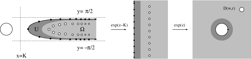
Figure 1. Preimages of a single disk under $F(z)=\exp(\exp(z-K))$.

The pair $(\Omega,F)$ is a model in the sense of [12], so by Theorem 1.1 of that paper, there is an $f\in\mathcal{B}$ and a quasiconformal homeomorphism $\varphi$ of the plane so that

1. $|f|\leq 1$ on the complement of $\Omega$,

2. $f\circ\varphi=F$ on $\Omega\setminus U$,

3. $\varphi$ is conformal except on $U$.

4. $S(f)\subset\overline{\mathbb{D}}$.

By condition (1), $f(\Omega^{c})\subset\overline{\mathbb{D}}\subset\Omega^{c}$, which implies $\Omega^{c}\subset\mathcal{F}(f)$. Thus, the Julia set of $f$ consists of points whose iterates stay in $\Omega$ forever.

Suppose $D=D(w,r)$ with $\operatorname{Re}(w)\geq K$ and $r\leq 4$ is a disk that hits $\mathcal{J}(f)$. Then the $f$-preimages of $D$ (i.e., the connected components of $f^{-1}(D)$) correspond $1$-to-$1$ to $F$-preimages via the map $\varphi$; more precisely, $f^{-1}(D)=\varphi(F^{-1}(D))$. Set $V=\{z\in\Omega:4<\operatorname{Re}(\exp(z-K))\}$. It is easy to check that

$$\int_{U}\frac{dxdy}{|z-w|^{2}}\leq C<\infty$$

for all $w\in V$ with a constant $C$ which is independent of $w$ and $r$. Because $\varphi$ is conformal off $U$, Lemma 15.1 of the current paper (applied to $A=U$ and $B=V$) implies that $\varphi$ is $L$-bi-Lipschitz on $V$ (where $L$ depends only on $C$ and the dilatation bound for $\varphi$) and hence also on the preimages of $D$ in question, at least if $K$ is large enough. Hence, the diameter of a connected component of $f^{-1}(D)$ is at most $M$ times the diameter of the corresponding component of $F^{-1}(D)$, and $M$ is independent of the disk $D$ and the choice of the preimage component.

The $F$-preimages of $D$ that are inside $\Omega$ can be understood in two steps: the inverses under $e^{z}$ consist of an infinite vertical “stack” of Jordan regions $\{W_{k}\}$ each of diameter $O(r/|w|)$ and each containing a point of the form $\log|w|+i(2\pi k+\arg(w))$, $k\in\mathbb{Z}$, see the center of Figure 1. The preimage of each $W_{k}$ is a region $U_{k}$ of diameter

$$O\left(\frac{r}{|w|(\log|w|+2\pi k)}\right),$$

and hence,

$$\sum_{k}\operatorname{diam}(U_{k})^{1+\delta}\leq\left(\frac{r}{|w|}\right)^{1+\delta}\sum_{k}\frac{1}{(\log|w|+2\pi|k|)^{1+\delta}}\leq\frac{Cr^{1+\delta}}{\delta|w|^{1+\delta}(\log|w|)^{\delta}}.$$

Using $|w|\geq K$, fixing $\delta>0$, and taking $K$ large (depending on $M$ below), we get

$$\sum\operatorname{diam}(U_{k})^{1+\delta}\leq\frac{r^{1+\delta}}{2M^{1+\delta}},$$

where the sum is over all preimages lying in $\Omega$. Thus,

$$\sum\operatorname{diam}(f^{-1}(D))^{1+\delta}\leq M^{1+\delta}\sum_{k}\operatorname{diam}(U_{k})^{1+\delta}\leq r^{1+\delta}/2.$$

This is (1.2) with $\epsilon=1/2$. We can also cover $\Omega$ by disks $\{B_{n}\}=\{D(n,4)\}_{n=K}^{\infty}$, and summing over all preimages of all these disks gives the sum

$$\sum_{n}\sum_{k}\operatorname{diam}(f^{-1}(B_{n}))^{1+\delta}=O\left(\sum_{n}\frac{1}{\delta|n|^{1+\delta}(\log K)^{\delta}}\right)<\infty,$$

i.e., (1.1). Thus, the Julia set of $f$ has dimension $\leq 1+\delta$, if $K$ is large enough. ∎

Our proof of Theorem 1.1 is significantly longer than the proof of Theorem 2.1 given above. Why? The approximation theorem for the Eremenko-Lyubich class from [12] has an analog for the Speiser class [13], but this result does not satisfy the crucial condition (1) above; if we attempt to approximate the function $F$ on the tract $\Omega$ by a Speiser class function $f$, we may be forced to make $f$ large at points outside $\Omega$ and this introduces many “extra” $f$-preimages that are not associated to any $F$-preimages, and we have no way to control them. Instead, we have to replace the tract $\Omega$ above by a more complicated region, and replace the approximation result from [12] by an application of the quasiconformal folding construction from [11].

The folding construction starts with a model function $F$ that is holomorphic on each connected component of the complement of an infinite, connected planar graph $T$, although it may be discontinuous across the edges of $T$. (In general, the graph need not be a tree, but we shall still denote it by “$T$” instead of “$G$”; in this paper the graph is an infinite tree except for a single closed loop). The function $F$ is modified in a certain neighborhood of $T$, denoted $T(r)$ (see next section), to give a quasiregular function $g$ on the plane that equals $F$ outside $T(r)$, and then $g$ is converted to an entire function $f=g\circ\varphi^{-1}$ with a quasiconformal homeomorphism $\varphi$ given by the measurable Riemann mapping theorem.

Suppose $\overline{T(2r)}\subset\mathcal{F}(f)$. Then the Julia set has a neighborhood $W$ disjoint from $T(2r)$ and $f=g\circ\varphi^{-1}=F\circ\varphi^{-1}$ on $W$. Moreover, we will show that $\varphi$ is bi-Lipschitz outside $T(2r)$ (Lemma 15.2). This means that for a disk $D$, connected components of $f^{-1}(D)$ can be associated via $\varphi$ to components of $F^{-1}(D)$ that have comparable size, and we will have good control of these components by construction. Thus, if we can build a model $F$ satisfying (1.1) and (1.2) with a small enough constant, then we will get a Speiser class entire function $f$ that also satisfies these conditions (with different constants) and this will imply Theorem 1.1.

The difficult part of this plan is the claim that $\overline{T(2r)}\subset\mathcal{F}(f)$. In our examples, the Fatou set will contain a large closed disk around the origin, and hence it will be enough to show that $f$ maps $T(2r)$ into this disk, i.e., that $f$ is bounded on $T(2r)$. This will reduce to showing that $F$ is bounded on $T(2r)$. The folding construction associates two positive weights, called the $\tau$-lengths, to each edge of the planar graph $T$ and it requires that the $\tau$-lengths of all edges in $T$ are uniformly bounded away from zero. Moreover, showing $F$ is bounded on $T(r)$ reduces to proving the $\tau$-lengths are uniformly bounded above. Essentially all the work in this paper is devoted to building a pair $(F,T)$ so that the function $F$ satisfies (1.1) and (1.2) and $\tau$-lengths for the graph $T$ are uniformly bounded above and away from zero. Once we have done this, the proof will proceed as in the Eremenko-Lyubich case described earlier.

In Section 3 we review quasiconformal folding; in Sections 4-8 we define the graph $T$ (and this determines $F$); in Sections 9-12 we give estimates of hyperbolic distances that culminate in the desired upper and lower bounds for $\tau$-length; in Sections 13-15 we estimate the correction map $\varphi$; and in Sections 16-18 we finish the proof of Theorem 1.1 and discuss the topology of the Julia set.

3. Quasiconformal folding

Quasiconformal folding is a technique for constructing transcendental entire functions with good control on both the singular values and the geometric behavior of the function. Here we will review some definitions and results from [11]; consult that paper for further details and proofs.

Let $f$ be a transcendental entire function with no finite asymptotic values and with only two critical values $\pm 1$. Then $T=f^{-1}([-1,1])$ is an unbounded, infinite tree and all components of $\Omega=\mathbb{C}\setminus T$ are unbounded, simply connected domains. We can choose a map $\tau$ which is conformal from each component of $\Omega$ onto the right half-plane $\mathbb{H}_{r}=\{x+iy:x>0\}$, and so that $f=\cosh\circ\,\tau$ on $\Omega$.

The idea of quasiconformal folding is to reverse this procedure. We start with an unbounded, infinite, locally finite tree $T$ which fulfills certain mild geometric conditions. Furthermore, for each component $\Omega_{j}$ of $\Omega=\mathbb{C}\setminus T$ let $\tau_{j}$ map $\Omega_{j}$ conformally onto $\mathbb{H}_{r}$ and let $\tau:\mathbb{C}\setminus T\to\mathbb{C}$ be given by $\tau=\tau_{j}$ on $\Omega_{j}$. The map $g$ given by $g=\cosh\circ\,\tau$ is then holomorphic off $T$. In general, $g$ is not continuous across $T$, but it is possible to change $g$ in a neighborhood

$$T(r)=\bigcup_{\text{edges }e\text{ of }T}\{z\in\mathbb{C}~{}:~{}\operatorname{dist}(z,e)<r\cdot\operatorname{diam}(e)\}$$

of $T$ so that it becomes continuous on the whole plane (the new function is quasi-regular on the plane). See Figures 2 and 3.

Figure 2. The $r$-neighbourhood of an arc $\gamma$ is the set given by $\gamma(r)=\{z:\operatorname{dist}(z,\gamma)<r\cdot\operatorname{diam}(\gamma)\}$ .

Figure 3. The neighbourhood of a graph is the union of neighborhoods of the individual edges.

Every edge $e$ of $T$ has two “sides” that are each mapped by $\tau$ to an interval on $i\mathbb{R}=\partial\mathbb{H}_{r}$. The $\tau$-size of $e$ is the minimum of the lengths of the two image intervals. For each component of $\Omega=\mathbb{C}\setminus T$, the sides of $T$ on $\partial\Omega$ correspond, via $\tau$, to a locally finite partition of $\partial\mathbb{H}_{r}$ into intervals. The folding theorem requires that there is a positive lower bound for the lengths of these intervals, usually taken to be $\pi$ (in many cases, we can replace $\tau$ by a positive multiple of itself, so the precise lower bound is not critical). The folding theorem also requires that adjacent intervals in these partitions have comparable lengths. This follows from bounded geometry, i.e., a planar graph has bounded geometry if (this is a slight strengthening of the conditions originally given in [11]):

1. the edges of $T$ are $C^{2}$ arcs with uniform bounds;

2. the union of edges meeting at a vertex are a bi-Lipschitz image of a star $\{z:z^{n}\in[0,r]\}$, i.e., a union of $n$ equally spaced, equal length radial segments meeting at $0$, with $n$ uniformly bounded;

3. for non-adjacent edges $e$ and $f$, $\operatorname{diam}(e)/\operatorname{dist}(e,f)$ is uniformly bounded.

Note that (2) implies adjacent edges have comparable lengths and that they meet at an angle bounded uniformly away from zero.

Theorem 3.1.

Suppose that $T$ has bounded geometry and every edge has $\tau$-size $\geq\pi$. Then there are $r>0,K>1$, an entire function $f$ and a $K$-quasiconformal map $\varphi$ so that $g=f\circ\varphi=\exp\circ\tau$ off $T(r)$. The constants $r$ and $K$ only depend on the bounded geometry constants of $T$. The only critical values of $f$ are $\pm 1$ and $f$ has no finite asymptotic values.

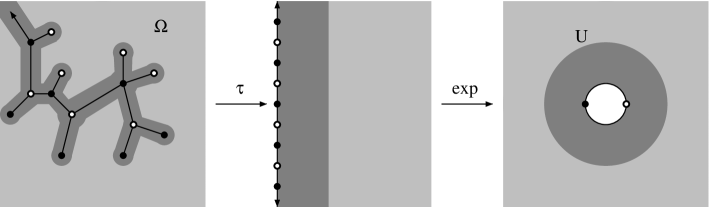
Figure 4. The quasiregular function $g$ equals the holomorphic function $\exp\circ\tau$ away from the tree (light gray) and is defined near the tree (dark gray) to be continuous and have bounded dilatation. The dilatation of the quasiconformal correction map is supported in this neighborhood of the tree.

This is Theorem 1.1 of [11], but we have modified the statement given there slightly. Here we have used “$\exp$” in place of “$\cosh$”; this is a harmless change, as explained in Section 7 of [13]. We can deduce a little more if we impose another geometric restriction on our bounded geometry tree:

Lemma 3.2.

Suppose that $T$ has bounded geometry and that $r$ is as in Theorem 3.1. Assume that for every edge $e$ of $T$, the neighbourhood $T_{e}(4r)=\{z\in\mathbb{C}~{}:~{}\operatorname{dist}(z,e)<4r\cdot\operatorname{diam}(e)\}$ only intersects edges whose length is comparable to the length of $e$ with constant $M$. Then there exists an $\epsilon>0$, only depending on $r$, the bounded geometry constants of $T$, and on $M$, so that for every point $z\in T(2r)$ there exists some edge $e^{\prime}$ so that the harmonic measure of $e^{\prime}$ with respect to $z$ is at least $2\epsilon$.

Proof.

Let $\Omega$ be one of the components of the complement of the tree, let $e$ be an edge on the boundary of $\Omega$, and let $z\in T_{e}(2r)\cap\Omega$. Let $e^{\prime}$ be the edge on the boundary of $\Omega$ which is closest to $z$. Then $e^{\prime}$ intersects $T_{e}(4r)$ and hence, by assumption, it has diameter comparable to the diameter of $e$. Let $d=\operatorname{dist}(z,e^{\prime})=O(\operatorname{diam}(e^{\prime}))$ and let $w\in e^{\prime}$ be a point closest to $z$. See the left side of Figure 5. By bounded geometry, there is a radius $r$ that is comparable to $\operatorname{diam}(e^{\prime})$ so that the disk $D(w,r)$ only hits $e^{\prime}$ or edges adjacent to $e^{\prime}$, of which there are only a bounded number. By the Beurling projection theorem (e.g., Theorem II.9.2 or Exercise II.10 of [20]) the part of $\partial\Omega$ in $D(w,r)$ has harmonic measure with respect to $z$ that is uniformly bounded away from zero. Since only a uniformly bounded number of edges hit this disk, one of them must have harmonic measure uniformly bounded away from zero, as desired. ∎

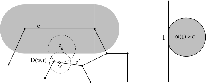
Figure 5. The proofs of Lemmas 3.2 and 3.3. The left side shows why there is an individual edge with large harmonic measure. The right side shows the region of large harmonic measure for an interval on the boundary of a half-plane.

Lemma 3.3.

Suppose that $T$ has bounded geometry and that $r$ is as in Theorem 3.1 and Lemma 3.2. Assume $T$ satisfies the assumption in Lemma 3.2. Suppose also that the $\tau$-lengths of all edges are bounded above. Then there exists $M<\infty$ so that $\tau(T(2r))\subset\{x+iy\in\mathbb{C}:0<x<M\}$. In other words, $|g|\leq e^{M}$ on $T(2r)$.

Proof.

Let $z\in T(2r)$ and let $e^{\prime}$ be the tree edge given by Lemma 3.2. Since $e^{\prime}$ has harmonic measure at least $2\epsilon$ with respect to $z$ in $\Omega$ (the complementary component of $T$ that contains $z$), one of the two sides of $e^{\prime}$ has harmonic measure at least $\epsilon$ with respect to $z$ in $\Omega$. Call this side $s^{\prime}$. By the conformal invariance of harmonic measure, $\omega(\tau(z),\tau(s^{\prime}),\mathbb{H}_{r})\geq\epsilon$. In the half-plane, the set of points at which a boundary interval $I$ has harmonic measure $\geq\epsilon$ is the intersection of a disk of radius $\simeq|I|/\epsilon$ with the half-plane. See the right side of Figure 5. Therefore $\tau(z)$ lies in this region. Since the $\tau$-lengths of all sides are bounded above, this implies $\tau(z)$ is within a bounded distance of the imaginary axis, i.e., $\tau(T(2r))$ is contained in a vertical strip of uniformly bounded width. ∎

If one wants a function that has finite asymptotic values, or that has critical points with high order, then the folding construction described above needs to be changed a bit. The tree $T$ is replaced by an unbounded, connected, locally finite graph. Each of the components $\Omega_{j}$ of $\Omega=\mathbb{C}\setminus T$ is one of three types (D, L or R), and each is mapped to a corresponding “standard” domain (disk, left half-plane or right half-plane) by a conformal map $\tau$. Each standard domain is then mapped by an associated holomorphic map $\sigma$. More precisely, the cases are:
$\bullet$ D-component: Here, $\Omega_{j}$ is a bounded domain whose boundary is a Jordan curve which consists of $d$ edges. D-components are quasiconformally mapped to $\mathbb{D}$ so that the $d$ vertices of the component map to $d$-th roots of unity. This is followed by the map $\sigma(z)=z^{d}$. This gives a critical value at $0$.
$\bullet$ L-component: $\Omega_{j}$ is an unbounded Jordan domain which is quasiconformally mapped to the left half-plane $\mathbb{H}_{l}$. This is followed by $\sigma(z)=\exp(z)$, which maps $\mathbb{H}_{l}$ to $\mathbb{D}$ and gives the asymptotic value $0$.
$\bullet$ R-component: These are the components which were used in the first theorem. Here, $\Omega_{j}$ is unbounded but not necessarily a Jordan domain. Each $\Omega_{j}$ is mapped onto $\mathbb{H}_{r}$ as before, and $\sigma(z)$ is $\exp(z)$.

Theorem 3.4.

Let $T$ be a bounded geometry graph and suppose $\tau$ is conformal from each complementary component of $T$ to the corresponding standard domain (i.e. $\mathbb{D}$, $\mathbb{H}_{l}$ or $\mathbb{H}_{r}$). Assume that

• D and L-components only share edges with R-components;

• on D-components with $n$ edges, $\tau$ maps the vertices to $n^{th}$ roots of unity;

• on L-components, $\tau$ maps sides to intervals of the form $[2\pi ki,2\pi(k+1)i]$;

• on R-components, the $\tau$-sizes of all edges are $\geq 2\pi$.

Then there exist $r>0$, $K>1$, an entire function $f$ and a $K$-quasiconformal map $\varphi$ of the plane so that $f\circ\varphi=\sigma\circ\tau$ off $T(r)$. The constants $r$ and $K$ only depend on the bounded geometry constants of $T$. Also, $S(f)=\{\pm 1\}$; plus $\{0\}$ if any D or L-components occur.

As before, if the $\tau$-sizes of the edges are bounded above by some constant $C$, we get that the image of the part of $T(2r)$ that lies in the R-components is mapped into a vertical strip whose width only depends on the bounded geometry constants and on $C$. The construction on the D and L-components can be modified to give singular values other than $0$, but we will not need this variation here.

4. The “trunk” of the tree

The graph to which we apply the folding theorem will be built in two steps. In this section, we present the first step: we construct a graph, called the “trunk”, that divides the plane into $4N+1$ connected components ($1$ D-component, $2N$ L-components, $2N$ R-components), where $N$ is a positive integer larger than $2$. In later sections, we will add “branches” (line segments) to the trunk, in order to get the “bounded $\tau$-length” condition.

The first of the $4N+1$ components is the disk $D(0,r_{N})$ where

$$r_{N}=\frac{1}{2\sin(\pi/(2N))}+N-1=N\left(1+\frac{1}{\pi}\right)-1+O\left(\frac{1}{N}\right).$$

This is the D-component and will be denoted $D_{0}$. Let $\theta=\frac{\pi}{N}$ and define

$$z_{k}=(r_{N}-N+1)\exp\left({i\left(\frac{\theta}{2}+k\theta\right)}\right)$$

for $0\leq k\leq 2N-1$. With $S_{0}=\{x+iy~{}:~{}x>0,|y|<1/2\}$ and $S_{k}=\exp(ik\theta)S_{0}$, the point $z_{k}$ is the unique non-zero intersection point between $\partial S_{k}$ and $\partial S_{k+1}$, see Figure 6. The L-components $L_{k}$ are then given by

$$L_{k} =\left\{z\in\mathbb{C}~{}:~{}|z-z_{k}|>N,\ k\theta<\arg(z-z_{k})<(k+1)\theta\right\}$$

$$=\left\{z_{k}+re^{i\phi}~{}:~{}r>N,\ k\theta<\phi<(k+1)\theta\right\}.$$

Note that these are truncated sectors that are disjoint, are unit distance apart, and are unit distance from the D-component, see Figure 6. The vertex of the $k$-th sector is $z_{k}$ (not the origin). One L-component is shown in light gray in Figure 6.

Finally, we construct the R-components. The complement $\Omega$ of the union of the D-component and L-components can be split into $2N$ congruent connected components $\{R_{k}\}$ by the radial segments

$$\left\{z\in\mathbb{C}:r_{N}\leq|z|\leq r_{N}+1,\ \arg(z)=\frac{\theta}{2}+k\theta\right\}.$$

Denote by $R_{0}$ the component in the right half-plane which is symmetric with respect to the real axis. The component $R_{k}$ for $1\leq k<2N-1$ is then the component which is just $R_{0}$ rotated by $\exp(ik\theta)$. Note that $R_{k}$ has a boundary arc on the circle of radius $r_{N}$ around the origin, two radial boundary arcs on the segments just defined, two circular arc boundary edges on the circles of radius $N$ around the points $z_{k-1}$ and $z_{k}$ (using $z_{-1}=z_{2N-1}$), and two sides that are infinite, parallel rays distance one apart, see Figure 6. Figure 7 shows the overall structure of the trunk graph.

Note that the five finite sides of the $R_{k}$ all have lengths comparable to $1$ and all the angles are approximately $90^{\circ}$, even as $N\to\infty$. These facts will help prove that our graph has bounded geometry with constants independent of $N$.

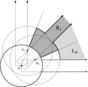
Figure 6. Consider $2N=8$ unit width half-strips rotated evenly around the circle. The D-component is a disk of radius $r_{N}$. The L-components are truncated sectors with vertices at the points where the half-strips intersect (one is shown in light gray). The remainder of the plane is divided into the R-components (one is shown in darker gray).

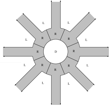
Figure 7. The “trunk” consisting of one D-component, $2N$ L-components that are truncated sectors, and an equal number of R-components that are essentially half-strips.

5. Conformal partition of the L-components

A conformal partition of an unbounded Jordan domain $\Omega$ is a collection of points $S$ on $\partial\Omega$ so that $\tau(S)\subset\partial H$ are evenly spaced, where $H$ is a half-plane and $\tau:\Omega\to H$ is a conformal map taking $\infty$ to $\infty$. For the L-components defined in Section 4 such a partition can be explicitly computed, and we record the computation in this section.

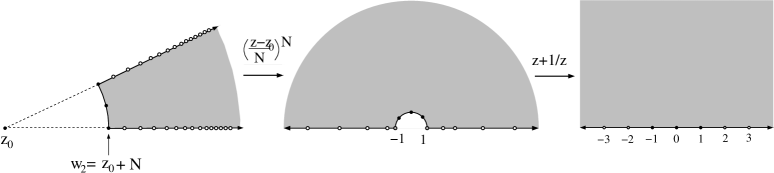
Figure 8. The L-components can be mapped to a half-plane by an explicit map (a rescaling and a power followed by the Joukowsky map), and thus the conformal partition is also given by explicit points.

The L-component $L_{0}$ is conformally mapped to the upper half-plane by

$$z\mapsto\left(\frac{1}{N}(z-z_{0})\right)^{N}+\frac{1}{\left(\frac{1}{N}(z-z_{0})\right)^{N}},$$

the composition of a linear rescaling, a power, and the Joukowsky map $z\mapsto z+1/z$, which conformally maps $\mathbb{H}\setminus\overline{\mathbb{D}}$ to $\mathbb{H}$, see Figure 8. The inverse map is given by

$$w\mapsto z_{0}+N\left(\frac{w}{2}+\sqrt{\left(\frac{w}{2}\right)^{2}-1}\right)^{1/N}=z_{0}+N\left(\frac{1}{2}\left(w+\sqrt{w^{2}-4}\right)\right)^{1/N}.$$

Let $w_{n}$ for $n\in\mathbb{Z}$ be the points on $\partial L_{0}$ that correspond under this map to the points of $\mathbb{Z}$ on the boundary of the upper half-plane. For $n\geq 2$ we define $t_{n}$ by the equation

$$w_{n}=z_{0}+N+t_{n}.$$

For $n\geq 2$, let $\Delta_{n}=t_{n+1}-t_{n}$. For convenience, we set $\alpha=1/N$ and define $\phi_{N}(n)=n^{2\sqrt{\alpha}}+2\log n$. Note that for fixed $n\geq 1$ this decreases as $N$ increases.

Lemma 5.1.

Suppose notation is as above. Then

(5.1) $$t_{n}=N(n^{\alpha}-1)+O\left(n^{\alpha-2}\right)$$

(5.2) $$t_{n}\leq N(n^{\alpha}-1)\leq Nn^{\alpha}\quad\text{and}\quad t_{n}\leq N(n^{\alpha}-1)\leq\phi_{N}(n),$$

(5.3) $$\Delta_{n}=n^{\alpha-1}+\frac{\alpha-1}{2}n^{\alpha-2}+O\left(n^{\alpha-3}\right),$$

(5.4) $$\Delta_{n}-\Delta_{n+1}=(1-\alpha)n^{\alpha-2}+O(n^{\alpha-3})=\Delta_{n}\left(\frac{1-\alpha}{n}+O(n^{-2})\right).$$

The big-$O$ estimates hold as $n\nearrow\infty$ and the constants in these inequalities do not depend on $N$.

Proof.

By definition (recall $\alpha=1/N$), if $n\geq 2$, then

$$w_{n} =z_{0}+N\left(\frac{1}{2}\left(n+\sqrt{n^{2}-4}\right)\right)^{\alpha}=z_{0}+Nn^{\alpha}\left(\frac{1}{2}\left(1+\sqrt{1-4n^{-2}}\right)\right)^{\alpha}$$

$$=z_{0}+Nn^{\alpha}\left(1+O\left(n^{-2}\right)\right)^{\alpha}=z_{0}+Nn^{\alpha}\left(1+O\left(\frac{1}{N}n^{-2}\right)\right)$$

$$=z_{0}+Nn^{\alpha}+O\left(n^{\alpha-2}\right).$$

The constants in the big-O’s hold as $n\nearrow\infty$ and they do not depend on $N$ since $\alpha=1/N\leq 1/2<1$ (in fact, one can easily check that the constant $4$ works). The equality in (5.1) is immediate. It is clear that the “O” term in the last line above is negative, so $t_{n}\leq N(n^{\alpha}-1).$ This gives the first part of (5.2). To prove the second part of (5.2), we consider two cases depending on whether $n$ is less than or greater than $N^{\sqrt{N}}$. For $1\leq n\leq N^{\sqrt{N}}$ we have

$$t_{n}\leq N(n^{\alpha}-1)=N(\exp(\alpha\log n)-1)\leq N(1+2\alpha\log n-1)=2\log n.$$

Here we have used the facts from calculus that $\alpha\log n\leq\sqrt{N}(\log N)/N\leq 1$ for $N\geq 3$ and $e^{x}\leq 1+2x$ for $0\leq x\leq 1$. For $n>N^{\sqrt{N}}$, since $\alpha\leq\sqrt{\alpha}$, we get

$$t_{n}\leq Nn^{\alpha}=Nn^{-\sqrt{\alpha}}n^{\alpha+\sqrt{\alpha}}\leq N\cdot N^{-\sqrt{N}/\sqrt{N}}n^{2\sqrt{\alpha}}=n^{2\sqrt{\alpha}}.$$

Since we have upper bounds on two disjoint intervals that cover all $n\geq 1$, we know $t_{n}$ is less than the sum of these two estimates. This is the second part of (5.2).

To compute the gaps $\Delta_{n}$ between the points $w_{n}$, we can omit the additive factor $z_{0}$ and consider the function

$$f(w)=N\left(\frac{1}{2}\left(w+\sqrt{w^{2}-4}\right)\right)^{\alpha}.$$

A calculus exercise shows (recall $\alpha N=1$):

$$f^{\prime}(w)= \left(\frac{1}{2}\left(w+\sqrt{w^{2}-4}\right)\right)^{\alpha-1}\cdot\frac{1}{2}\left(1+w\left(w^{2}-4\right)^{-1/2}\right)$$

$$=w^{\alpha-1}\left(\frac{1}{2}+\frac{1}{2}\sqrt{1-4w^{-2}}\right)^{\alpha-1}\cdot\frac{1}{2}\left(1+w\left(w^{2}-4\right)^{-1/2}\right)$$

$$=w^{\alpha-1}\left(1+O\left(\frac{1}{w^{2}}\right)\right)^{\alpha-1}\left(1+O\left(\frac{1}{w^{2}}\right)\right)$$

$$=w^{\alpha-1}+O\left(w^{\alpha-3}\right).$$

tends to zero as $w\to\infty$. A similar computation shows that

$$f^{\prime\prime}(w)=(\alpha-1)w^{\alpha-2}+O(w^{\alpha-4}).$$

Using Taylor series, we see that

$$\Delta_{n}=f(n+1)-f(n) = \int_{n}^{n+1}f^{\prime}(t)dt,$$

$$= \int_{n}^{n+1}\left[n^{\alpha-1}+(\alpha-1)(t-n)n^{\alpha-2}+O(n^{\alpha-3})\right]dt,$$

$$= n^{\alpha-1}+\frac{1}{2}(\alpha-1)n^{\alpha-2}+O\left(n^{\alpha-3}\right),$$

which is (5.3). Finally, using the mean value theorem gives (5.4):

$$\Delta_{n}-\Delta_{n+1} = \left[n^{\alpha-1}+\frac{\alpha-1}{2}n^{\alpha-2}+O\left(n^{\alpha-3}\right)\right]$$

$$\qquad\qquad-\left[(n+1)^{\alpha-1}+\frac{\alpha-1}{2}(n+1)^{\alpha-2}+O\left(n^{\alpha-3}\right)\right]$$

$$= \left[n^{\alpha-1}-(n+1)^{\alpha-1}\right]+\frac{1}{2}(\alpha-1)\left[n^{\alpha-2}-(n+1)^{\alpha-2}\right]+O\left(n^{\alpha-3}\right)$$

$$= (1-\alpha)n^{\alpha-2}+O\left(n^{\alpha-3}\right).\qed$$

Since $\{\phi_{N}\}$ is decreasing in $N$, $\{t_{n}\}$ has an upper bound independent of $N$, and this bound improves if $N$ is large, e.g., if $N\geq 16$, then $t_{n}\leq\phi_{16}(n)=\sqrt{n}+2\log n.$

Corollary 5.2.

With notation as above, if $0<\delta\leq 1$ and $N>2\left(1+\frac{1}{\delta}\right)$, then

$$\sum_{n=1}^{\infty}\Delta_{n}^{1+\delta}=O\left(\frac{1}{\delta}\right),$$

where the constant does not depend on $N$.

Proof.

After some arithmetic, we see that the hypothesis $N>2(1+1/\delta)$ is equivalent to $(\alpha-1)(1+\delta)<-1-\frac{\delta}{2},$ and after some calculus, (5.3) implies

$$\sum_{n=1}^{\infty}\Delta_{n}^{1+\delta}=O\left(\sum_{n=1}^{\infty}n^{-1-\frac{\delta}{2}}\right)=O\left(\frac{1}{\delta}\right).\qed$$

6. The “branches” of the tree

We modify the components $R_{k}$ by adding line segments perpendicular to the boundary as illustrated in Figure 9. We describe the construction of the R-components only for the component $R_{0}$ intersecting the positive real axis; the other R-components will all be rotations of this one.

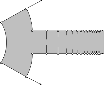
Figure 9. An R-component and the conformal partition points coming from the two adjacent L-components. The spikes get shorter and closer together near $\infty$, but they do not accumulate at any finite point.

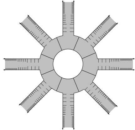
Figure 10. The final shape of the graph with all the slits attached. The vertices on the slits (defined in Section 8) are too close together to see at this scale.

We define the modified R-component $\Omega_{0}\subset R_{0}$ by removing vertical slits that are attached to the top and bottom edges of $R_{0}$ at the partition points of the adjacent L-components; these points were described in Section 5. The region between two adjacent slits will be informally referred to as a “tower”; it is the trapezoid defined by the two slits and the connecting segment on the boundary of $R_{0}$. The slits will be chosen so that the domain $\Omega_{0}$ is symmetric with respect to the real line. Thus, it suffices to define the length of the slit attached to the point $w_{n}=z_{0}+N+t_{n}$ on the top edge of $\Omega_{0}$ (the top edge is the horizontal ray starting at $w_{2}=z_{0}+N$).

The segment attached at the partition point $w_{n}$ is denoted $\lambda_{n}$ and has length

(6.1) $$y_{n}=\min\left\{\frac{1}{4},\Delta_{n}\left(t_{n}+\frac{1}{\pi}\log\Delta_{n}\right)\right\}.$$

If $y_{n}<1/4$, then by Lemma 5.1 we have

(6.2) $$t_{n}=\frac{y_{n}}{\Delta_{n}}-\frac{\alpha-1}{\pi}\log n+O\left(n^{\alpha-2}\right)=\frac{y_{n}}{\Delta_{n}}-\frac{\alpha-1}{\pi}\log n+O\left(\frac{1}{n}\right)$$

because $\alpha-2=\frac{1}{N}-2<-1$. We will later interpret this equation as an equality (up to a bounded additive factor) between two hyperbolic distances in $\Omega_{0}$; see Corollary 12.7. This approximate equality will imply that the desired $\tau$-length upper and lower bounds in Theorem 3.4 hold. See Lemma 12.8.

Lemma 6.1.

We have $y_{n}<1/4$ for $n\geq n_{0}$, with $n_{0}$ independent of $N$.

Proof.

From Lemma 5.1 we know that

$$N(n^{\alpha}-1)\leq\phi_{N}(n)=n^{2\sqrt{\alpha}}+2\log n.$$

Since $\{\phi_{N}\}$ is decreasing (and $\frac{1}{20}+\frac{2}{\sqrt{20}}-1<-\frac{1}{2}$), if $N\geq 20$, then

$$y_{n}=\Delta_{n}\left(t_{n}+\frac{1}{\pi}\log\Delta_{n}\right) = O\left(n^{\alpha-1}(\phi_{N}(n)+\log n)\right)$$

$$= O\left(n^{\alpha+2\sqrt{\alpha}-1}+n^{\alpha-1}\log n\right)$$

$$= O\left(n^{-1/2}\right).\qed$$

Thus, only finitely many segments will have length $1/4$ and this number is bounded independent of $N$. Let $\epsilon_{n}=\min\{\frac{1}{4},C_{1}/\sqrt{n}\}$, for $n\geq 2$, where $C_{1}$ is chosen so that $y_{n}\leq\epsilon_{n}$ for all $n\geq 2$. Define $\epsilon(t_{n})=\epsilon_{n}$ and define $\epsilon(t)$ for $t_{n}\leq t\leq t_{n+1}$ by linear extension. This function is continuous and decreasing, and we have $\Omega_{1}\subset\Omega_{0}\subset R_{0}$ where

$$\Omega_{1}=\left\{(t+\operatorname{Re}z_{0}+N)+iy:t>0,|y|<\frac{1}{2}-\epsilon(t)\right\}.$$

Recall that $t_{2}=0$ so that $\epsilon$ is in fact defined on $[0,\infty)$.

Lemma 6.2.

If $N\geq 20$, then $\int_{0}^{\infty}\epsilon(t)dt<\infty$ with a bound that is independent of $N$.

Proof.

Choose $n_{0}$ so that $\epsilon_{n}=C_{1}/\sqrt{n}$ for $n\geq n_{0}$. By Lemma 5.1,

$$\int_{0}^{\infty}\epsilon(t)dt \leq\sum_{n=2}^{\infty}\epsilon(t_{n})\Delta_{n}=\sum_{n=2}^{n_{0}-1}\frac{\Delta_{n}}{4}+\sum_{n=n_{0}}^{\infty}\frac{C_{1}\Delta_{n}}{\sqrt{n}}$$

$$\leq C_{2}+C_{3}\sum_{n=n_{0}}^{\infty}n^{\alpha-\frac{3}{2}}\leq C_{2}+C_{3}\sum_{n=n_{0}}^{\infty}n^{-\frac{4}{3}}<\infty.\qed$$

This will be used in Corollary 10.3 to approximate hyperbolic distance in $\Omega_{0}$.

7. $\{y_{n}\}$ is almost convex

Imagine that we connect the endpoints of adjacent vertical slits by segments to form an infinite polygonal path. We want to verify that this path is “not far” from being convex. More precisely, define $s_{n}=(y_{n}-y_{n+1})/\Delta_{n}$; this is the slope of the segment connecting the endpoints of the $n^{\text{th}}$ and $(n+1)^{\text{st}}$ slits. The quantity $(s_{n}-s_{n+1})/\Delta_{n}$ is thus a type of second derivative, and can be thought of as the curvature of the polygonal path. The path will be convex down if all these numbers are negative. This is true, but tedious to prove; we will give an easier estimate that is sufficient for our needs. Recall that $\phi_{N}(n)=n^{2\sqrt{\alpha}}+2\log n$, $\alpha=1/N$.

Lemma 7.1.

Suppose $N\geq 24$. There is a $n_{0}>0$, independent of $N$, so that for $n\geq n_{0}$, $s_{n}$ is decreasing to zero, and

$$|s_{n}-s_{n+1}|=O\left(\phi_{16}(n)/n^{2}\right)=O\left(n^{2\sqrt{1/16}-2}\right)+O\left(n^{-2}\log n\right)=O\left(n^{-3/2}\right),$$

with constants independent of $N$. In particular, $|s_{n}-s_{n+1}|=o\left(n^{\alpha-1}\right)=o\left(\Delta_{n}\right)$.

Proof.

We simply compute using the definitions. Recall that $t_{n+1}=t_{n}+\Delta_{n}$. For notational convenience, let $\kappa_{1}=(1-\alpha)/\pi$, $\kappa_{2}=\frac{1-\alpha}{2}$, and let $\phi=\phi_{16}$. If $n$ is large enough, we get from (6.1)

$$s_{n} =\frac{y_{n}-y_{n+1}}{\Delta_{n}}=\frac{\Delta_{n}(t_{n}+\frac{1}{\pi}\log\Delta_{n})-\Delta_{n+1}(t_{n+1}+\frac{1}{\pi}\log\Delta_{n+1})}{\Delta_{n}}$$

$$=t_{n}+\frac{1}{\pi}\log\Delta_{n}-\left(1-\frac{\Delta_{n}-\Delta_{n+1}}{\Delta_{n}}\right)\left(t_{n}+\Delta_{n}+\frac{1}{\pi}\log\Delta_{n+1}\right)$$

$$=-\Delta_{n}+\frac{1}{\pi}(\log{\Delta_{n}}-\log{\Delta_{n+1}})+\left(\frac{\Delta_{n}-\Delta_{n+1}}{\Delta_{n}}\right)\left(t_{n}+\Delta_{n}+\frac{1}{\pi}\log\Delta_{n+1}\right).$$

Now use Lemma 5.1 to note that

$$\log\Delta_{n}=\log\left(n^{\alpha-1}\left(1+\frac{\alpha-1}{2n}+O\left(n^{-2}\right)\right)\right)=\left(\alpha-1\right)\log n-\frac{\kappa_{2}}{n}+O\left(n^{-2}\right).$$

Using this we get

$$s_{n} =-\Delta_{n}-\kappa_{1}\log\frac{n}{n+1}+O(n^{-2})$$

$$\qquad\qquad+\frac{\Delta_{n}-\Delta_{n+1}}{\Delta_{n}}\left[t_{n}+\Delta_{n}-\kappa_{1}\log(n+1)+O(n^{-1})\right]$$

$$=-\Delta_{n}+\frac{\kappa_{1}}{n}+\left(\frac{\kappa_{2}}{n}+O(n^{-2})\right)\left[t_{n}+\Delta_{n}-\kappa_{1}\log(n+1)+O(n^{-1})\right]+O(n^{-2})$$

$$=-\Delta_{n}+\frac{\kappa_{1}}{n}+\kappa_{2}\frac{t_{n}}{n}-\kappa_{1}\kappa_{2}\frac{\log(n+1)}{n}+O\left(\phi(n)/n^{2}\right),$$

where we have used $\Delta_{n}/n=O\left(n^{\alpha-2}\right)=O\left(\phi(n)/n^{2}\right)$. This shows that $s_{n}\to 0$.

We now want to estimate $|s_{n}-s_{n+1}|$. The big-O term is already the correct size, and taking differences preserves this. Next, note we have already shown in (5.4) that

$$\Delta_{n}-\Delta_{n+1}=O\left(n^{\alpha-2}\right)=O\left(\phi(n)/n^{2}\right).$$

Since we assumed $N\geq 24$ we have $\alpha=1/N<1/4$, so using (5.2) and (5.3) and ignoring the multiplicative factor we get

$$\frac{t_{n}}{n}-\frac{t_{n+1}}{n+1} ={t_{n}}\left(\frac{1}{n}-\frac{1}{n+1}\right)+\frac{t_{n}-t_{n+1}}{n+1}$$

$$=O\left({t_{n}}n^{-2}\right)+O\left(\frac{\Delta_{n}}{n+1}\right)$$

$$=O\left(\phi(n)/n^{2}\right).$$

Similar arguments complete the proof by showing

$$\frac{1}{n}-\frac{1}{n+1} = O\left(\frac{1}{n^{2}}\right)=O\left(\phi(n)/n^{2}\right),$$

$$\frac{\log(n+1)}{n}-\frac{\log(n+2)}{n+1} = O\left(\frac{\log n}{n^{2}}\right)=O\left(\phi(n)/n^{2}\right).\qed$$

Next we derive a geometric consequence:

Corollary 7.2.

For $n>n_{0}$ (as in the previous lemma) the endpoints of the $n^{\text{th}}$ and $(n+1)^{\text{st}}$ slits are on the boundary of an open disk $D_{n}$ in $\Omega$ centered on the axis of $\Omega$. Furthermore, there is a disk $B_{n}$ whose radius is bounded below independently of $N$ and $n$ containing the endpoints of the $n^{\text{th}}$ and $(n+1)^{\text{st}}$ so that no other endpoint lies within $\overline{B_{n}}$. The boundary of $B_{n}$ intersects all slits within unit distance of the $n^{\text{th}}$ slit in either direction.

Proof.

Note that a disk which is centered on the real line and completely contained in the R-component has radius at most $\frac{1}{2}$. In particular, the curvature of such a disk is at least $2$. This means that slope of the circle (considered as the graph of a function) changes by at least $\simeq\Delta$ over a horizontal distance $\Delta$ (the change is smallest when the interval is centered around the center of the disk), see Figure 11. On the other hand, we can choose $n_{0}$ in the Lemma 7.1 so that the curvature of the polygonal path through the endpoints of the slits with indices larger than $n_{0}$ is much less than $2$. Thus if we move from the $(n+1)$st tip to the right, the path can never intersect the boundary of this disk again. If it did, then there would be a segment of the path whose slope is less than or equal to the slope of $\partial D$ at the point of intersection, and this is impossible by observations above. A similar argument works to the left of the $n$-th tip. This proves the existence of the disk $D_{n}$.

Figure 11. Existence of $D_{n}$. By definition one segment of our path forms a chord of the disk $D_{n}$. The slope of the circle changes by at least a fixed amount proportional to the horizontal distance from this chord, and the slopes of the path segments change at most by a much smaller multiple of this distance. Thus the path cannot intersect the disk except along the given segment.

We simply define $B_{n}$ to be the largest disk the boundary of which passes through the endpoints of the $n^{\text{th}}$ and $(n+1)^{\text{st}}$ slits and lies above the polygonal path unlike $D_{n}$ which lies below that path, see Figure 12. Since the curvature of the polygonal path is bounded above, we get an upper bound for the curvature of the boundary of $B_{n}$ and thus a lower bound for the radius. We can ensure that the boundary of this disk intersects all slits within unit distance of the $n^{\text{th}}$ slit in either direction by increasing $n_{0}$ and thus increasing the minimal radius of $B_{n}$ if needed. ∎

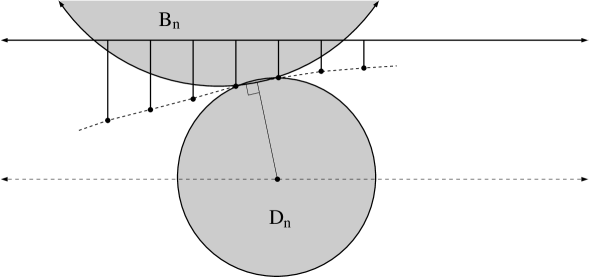
Figure 12. Existence of $B_{n}$. The dashed curved connecting the slit tips lies between two disks with radius bounded uniformly away from zero. Later we will use this to estimate the hyperbolic distance from the axis to points near the tips of the slits.

A stronger result holds: $s_{n}\searrow 0$. This implies that the polygonal curve is convex and hence the disk $B_{n}$ in Lemma 7.2 can be taken to be a half-plane. However, verifying this seems to require long and tedious computations, so we omit the proof, since the weaker condition above is sufficient for our purposes.

8. The definition of $T$

We finally come to the definition of the graph $T$. In the previous section we have built a graph by defining the “trunk” and adding “branches”. As a planar set, this is $T$, but to make $T$ a graph we have to specify the vertices. The vertices along the trunk have already been given; in this section we define the vertices on the branches. Once this is done, $T$ has been completely specified.

Divide the slit $\lambda_{n}$ attached to the trunk at position $w_{n}$ into disjoint segments of length $\Delta_{n}$, except the last segment at the end of the slit closest to the axis, which has length between $\Delta_{n}$ and $2\Delta_{n}$. By (6.1), $\lambda_{n}$ is divided into

$$m_{n}=\left\lfloor\frac{y_{n}}{\Delta_{n}}\right\rfloor=\left\lfloor t_{n}+\frac{1}{\pi}\log\Delta_{n}\right\rfloor.$$

many pieces. Note,

$$\frac{y_{n+1}}{\Delta_{n+1}}-\frac{y_{n}}{\Delta_{n}}=\left(t_{n+1}+\frac{1}{\pi}\log\Delta_{n+1}\right)-\left(t_{n}+\frac{1}{\pi}\log\Delta_{n}\right)=\Delta_{n}+\frac{1}{\pi}\log\frac{\Delta_{n+1}}{\Delta_{n}}\to 0$$

so $|m_{n+1}-m_{n}|\leq 1$ for large $n$.

Next, we add $\lfloor\exp(\pi k)\rfloor$ vertices to the $k$-th segment (the one that is distance $k\cdot\Delta_{n}$ from $w_{n}$, the point where the slit is attached to the trunk). Thus, the spacing between vertices in the $k$-th segment is $\simeq\Delta_{n}\exp(-\pi k)$. We do something slightly different in the last segment at the end of the slit. Instead of adding vertices evenly spaced in that last interval, we use a square root to place the points, as in Figure 13, so that the spacing changes from $\exp(-\pi m_{n})\Delta_{n}$ (away from the tip) to $\exp(-\pi m_{n}/2)\Delta_{n}$ (at the tip). This implies that all these edges have comparable $\tau$-length.

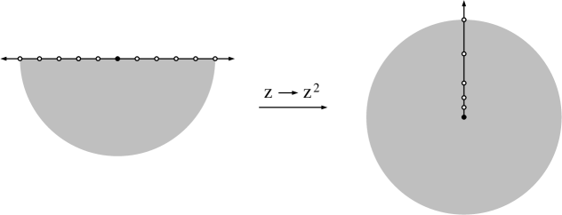
Figure 13. Placing points near the tip of a slit. The even spacing on the left is mapped to an uneven spacing on the right that gives all the sides comparable $\tau$-length.

Lemma 8.1.

$T$ has bounded geometry with constants independent of $N$.

Proof.

The graph was constructed so this would be true, but we briefly review the different conditions. First, all the edges are either straight line segments or circular arcs with bounded curvature, independent of $N$; the angles between adjacent edges are $\pi/2$ or $\pi$ and the valence of the vertices is at most $3$; and adjacent edges have comparable lengths by construction. From these facts we easily deduce that (1) and (2) of the bounded geometry conditions hold.

It remains to show that for non-adjacent edges $e$ and $f$ the ratio $\operatorname{diam}(e)/\operatorname{dist}(e,f)$ is uniformly bounded. But again, this holds by construction. The edges have either a distance of at least $1/2$ (when they lie on different sides of the symmetry line of $\Omega$) or they lie on the same side of the symmetry line. In this case, they lie either on opposite sites of one of the “towers” or on sides of different towers even further apart. But then the diameter of the edges is bounded by the width of the tower, which is a lower bound for the distance between the edges. If the edges lie on the same slit, then the boundedness follows since adjacent edges have uniformly comparable length and there is at least one edge in between the two edges under consideration. ∎

We also need to know that our graph satisfies the condition in Lemma 3.3:

Lemma 8.2.

For every edge $e$ of $T$, and any $r>0$ the neighbourhood $T_{e}(4r)=\{z\in\mathbb{C}~{}:~{}\operatorname{dist}(z,e)<4r\cdot\operatorname{diam}(e)\}$ only intersects edges whose length is comparable to the length of $e$.

We leave the (simple) proof to the reader.

9. Estimates for the hyperbolic metric

Now that we have defined $T$ (and hence the model function $F$), our next goal is to prove that it satisfies the $\tau$-length upper and lower bounds discussed earlier. This reduces to careful estimates of hyperbolic length within the R-components. We start with a review of some basic facts that can be found, for example, in [20]. The hyperbolic length of a (Euclidean) rectifiable curve in the unit disk $\mathbb{D}$ is given by integrating

$$\frac{ds}{1-|z|^{2}},$$

along the curve. In the upper half-plane $\mathbb{H}$ we integrate ${ds}/{2y}$. Note that this definition differs by a factor of $2$ from that given in some sources, e.g., [6], which contains estimates similar to the ones we will derive below.

The hyperbolic distance between two points is given by taking the infimum of all hyperbolic lengths of paths connecting the points. In the disk, minimizers (hyperbolic geodesics) are either diameters of the disk or subarcs of circles perpendicular to the unit circle. In the upper half-plane, the hyperbolic geodesics are either vertical rays or semi-circles centred on the real line. The hyperbolic distance between two points $z,w$ is given by

$$\rho(z,w)=\frac{1}{2}\log\frac{1+T(z,w)}{1-T(z,w)},$$

where

$$T(z,w)=\left|\frac{z-w}{1-\overline{w}z}\right|,\qquad T(z,w)=\left|\frac{z-w}{z-\overline{w}}\right|,$$

for $\mathbb{D}$ and $\mathbb{H}$, respectively. For the disk, taking $z=0$, $w=r=1-\epsilon>0$ gives

(9.1) $$R=\rho(0,r)=\frac{1}{2}\log\frac{1+r}{1-r}=\frac{1}{2}\log\frac{2-\epsilon}{\epsilon}.$$

Therefore, $\epsilon=2/(1+\exp(2R))$, which gives $\exp(-2R)\leq\epsilon\leq 2\exp(-2R).$

Koebe’s estimate (e.g., Theorem I.4.3 of [20]) says that if $\varphi$ is conformal from $\mathbb{D}$ to a simply connected domain $\Omega$, then

$$\frac{1}{4}|\varphi^{\prime}(z)|(1-|z|^{2})\leq\operatorname{dist}(\varphi(z),\partial\Omega)\leq|\varphi^{\prime}(z)|(1-|z|^{2}).$$

The hyperbolic metric $\rho=\rho_{\Omega}$ on a simply connected planar domain $\Omega$ is defined by transferring the hyperbolic metric on $\mathbb{D}$ by a conformal map (the choice of the map makes no difference). The quasi-hyperbolic metric on $\Omega$ is defined by integrating

$$d\widetilde{\rho}=\frac{ds}{\operatorname{dist}(z,\partial\Omega)}.$$

Koebe’s estimate implies these two metrics are comparable to within a factor of $4$,

$$\rho_{\Omega}(z,w)\leq\widetilde{\rho}_{\Omega}(z,w)\leq 4\cdot\rho_{\Omega}(z,w).$$

In particular, if $L$ is a line segment and $\operatorname{dist}(L,\partial\Omega)\simeq\operatorname{diam}(L)$, then $L$ has hyperbolic length comparable to $1$.

Another domain for which we can explicitly compute the hyperbolic metric is the infinite strip $S=\{(x,y):|y|<1/2\}$. This is conformally mapped to $\mathbb{H}_{r}$ by $\exp(\pi z)$, so a simple computation shows that the hyperbolic metric on $S$ is given by $d\rho=\frac{\pi}{2}ds/\cos(\pi y)$. From this we can deduce that for $|y|<1/2$, we have

(9.2) $$\rho_{S}(x,x+iy)=\frac{\pi}{2}\int_{0}^{|y|}\frac{ds}{\cos(\pi s)}=\frac{\pi}{2}\log\frac{1}{\frac{1}{2}-|y|}+O(1).$$

The geodesics in $S$ are a little difficult to draw, but some of them can be well approximated by a polygonal arc as follows:

Lemma 9.1.

If $z=x+i0$, $w=s+it$, $|t|<1/2$, and $p=s+i0$, then

$$\rho_{S}(z,w)=\rho_{S}(z,p)+\rho_{S}(p,w)+O(1)=\frac{\pi}{2}|x-s|+\frac{\pi}{2}\log\frac{1}{\frac{1}{2}-|t|}+O(1).$$

Proof.

One direction is obvious by the triangle inequality and (9.2). To prove the other direction, we can use conformal invariance to replace $S$ by $\mathbb{D}$, set $p=0$ and assume $z$ is on the segment from $0$ to $i$ and $w$ is on the segment from $0$ to $1$. See Figure 14. The geodesic $\gamma$ from $z$ to $w$ must hit the Euclidean ball $D=D(0,\sqrt{2}-1)$. Note that $D\cap\gamma$ has hyperbolic length $O(1)$ and the segments of $\gamma\setminus D$ (if any) are longer than $\rho(w,D)=\rho(w,0)-O(1)$ and $\rho(z,0)=\rho(0,z)-O(1)$. This proves the result. ∎

Figure 14. Proof of Lemma 9.1. The geodesic is only $O(1)$ shorter than the polygonal path.

Lemma 9.2.

If $W_{1}\subset W_{2}$ are simply connected domains, $z\in W_{1}$, and $R=\rho_{W_{2}}(z,W_{2}\setminus W_{1})\geq c>0$, then

$$\rho_{W_{2}}(z)\leq\rho_{W_{1}}(z)\leq(1+O(e^{-2R}))\rho_{W_{2}}(z),$$

where the constant in the “big-O” only depends on $c$.

Proof.

The left inequality is a well known consequence of the Schwarz lemma. To prove the right side, we may assume using conformal invariance that $W_{2}=\mathbb{D}\subset W_{1}/(1-\epsilon)$ where $R$ and $\epsilon$ are as in (9.1). Thus

$$\rho_{W_{2}}(0)\leq\rho_{W_{1}}(0)/(1-\epsilon)\leq\rho_{W_{1}}(0)(1+O(\epsilon))\leq\rho_{W_{1}}(0)(1+O(\exp(-2R))),$$

if $\epsilon<1$ or $R>0$ uniformly. ∎

For an even more precise version of Lemma 9.2, see Proposition 3.4 of [28].

Lemma 9.3.

Suppose $I,J$ are disjoint intervals on the boundary of $\mathbb{H}_{r}$ and suppose $\gamma_{I},\gamma_{J}$ are the hyperbolic geodesics that have the same endpoints as $I$ and $J$ respectively. Suppose $\gamma$ is the geodesic that connects the center of $I$ to $\infty$ ($\gamma$ is a horizontal ray). Let $z$ be the point on $\gamma$ that is closest to $\gamma_{J}$ with respect to the hyperbolic metric in the right half-plane. If $\rho(z,\gamma_{J})=\rho(z,\gamma_{I})+C$, then $|I|\simeq|J|$ with a multiplicative factor depending only on $C$.

Proof.

See Figure 15. Map $\mathbb{H}_{r}$ to $\mathbb{D}$ by a Möbius transformation $\tau$ that sends the center of $I$ to $-1$, $z$ to $0$ and $\infty$ to $1$. It is easy to check the images of $I$ and $J$ have comparable length on the circle, and that the image of $J$ is bounded away from $1$. This implies $I$ and $J$ have comparable length on $i\mathbb{R}$ because the derivative of $\tau^{-1}$ has comparable absolute values on $I$ and $J$. ∎

           

Figure 15. Proof of Lemma 9.3.

Lemma 9.4.

Suppose $Q$ is an open square with center $q$, and $\Omega\supset Q$ is a simply connected region such that $\partial\Omega$ contains the top and bottom sides of $Q$ and $\Omega$ contains the left and right sides of $Q$. Then $\Omega\setminus Q$ has two connected components, separated by $Q$. Suppose that $a,b$ are in different components. Let $\gamma$ be the hyperbolic geodesic in $\Omega$ connecting $a$ and $b$. Then $\rho_{\Omega}(\gamma,q)=O(1)$.

Proof.

Let $I$ and $J$ be the top and bottom sides of $Q$. Let $\sigma_{I},\sigma_{J}$ be the hyperbolic geodesics for $Q$ joining the endpoints of $I$ and $J$ respectively, and let $\gamma_{I}$, $\gamma_{J}$ be the hyperbolic geodesics for $\Omega$ joining the same pairs of points, see Figure 16.

It is a standard fact that $\sigma_{I}$ are exactly the points $z$ in $Q$ where $I$ has harmonic measure $1/2$ (the solution of the Dirichlet problem with boundary values $1$ on $I$ and zero on $\partial Q\setminus I$). Since $Q\subsetneq\Omega$, the maximum principle for harmonic functions implies that the harmonic measure of $I$ in $\Omega$ will be $>1/2$ at each point of $\sigma_{I}$, and therefore $\gamma_{I}$ is separated from $I$ in $\Omega$ by $\sigma_{I}$. Similarly for $\gamma_{J}$ and $\sigma_{J}$. See Figure 16.

Finally, distinct hyperbolic geodesics in a simply connected domain either intersect once or not at all and any intersection is a crossing (this is obvious in the disk or half-plane model). Hence, $\gamma$ does not intersect either $\gamma_{I}$ or $\gamma_{J}$ (it could not connect $a$ to $b$ if it crossed either curve only once). Therefore it crosses $Q$ traveling between $\sigma_{I}$ and $\sigma_{J}$ and hence comes within $O(1)$ of the center point $q$ (a simple argument leads to the explicit estimate $\rho_{\Omega}(\gamma,q)\leq\rho_{Q}(\sigma_{I},q)=\frac{1}{2}\log\sqrt{2}/(2-\sqrt{2})\approx.4407$). ∎

Figure 16. A geodesic $\gamma$ for $\Omega$ crossing $Q$ horizontally passes between the geodesics $\sigma_{I}$, $\sigma_{J}$ for $Q$ corresponding to the top and bottom of $Q$. Thus $\gamma$ comes within a fixed distance of the center $q$.

10. The hyperbolic metric in approximate rectangles

Lemma 10.1.

Fix $t>0$, set $R=\{(x,y):0<x<t,|y|<1/2\}$ and suppose $\Omega\supset R$ is a simply connected domain whose boundary contains the top and bottom sides of $R$. Then

$$\rho_{\Omega}(a,b)=\frac{\pi}{2}(b-a)+O(1)$$

whenever $0<a<b<t$ and $a,(t-b)$ are both bounded away from zero.

Proof.

First consider $\Omega=R$. Note that $R\subset S=\{(x,y):|y|<1/2\}$, so $d\rho_{R}\geq d\rho_{S}$ by one direction of Lemma 9.2. On the interval $[a,b]$, the other direction gives

$$d\rho_{R}(x) \leq (1+O(\exp(-2\rho_{S}(x,S\setminus R))))\cdot d\rho_{S}(x)$$

$$\leq (1+O(\exp(-\pi\min(x,t-x))))\cdot\frac{\pi}{2}dx.$$

Integrating from $a$ to $b$ gives $\rho_{R}(a,b)=\frac{\pi}{2}(b-a)+O(1).$

For a general $\Omega$, we repeat this argument with $S$ replaced by $\Omega$ to get

$$d\rho_{R}(x)/(1+O(\exp(-2\rho_{\Omega}(x,\Omega\setminus R))))\leq d\rho_{\Omega}(x)\leq d\rho_{R}(x),$$

for $a<x<b$. By Koebe’s theorem $\rho_{\Omega}(x,\Omega\setminus R)\simeq\min(x,t-x),$ so integrating gives

$$\rho_{\Omega}(a,b)=\rho_{R}(a,b)+O(1)=\frac{\pi}{2}(b-a)+O(1).\qed$$

Recall the definitions of $\Omega_{0}$ and $\Omega_{2}$ from Section 6 ($\Omega_{0}$ was defined in the second paragraph and $\Omega_{1}$ just before Lemma 6.2).

Lemma 10.2.

Suppose $\epsilon(t)$ and $\Omega_{1}$ are as in Lemma 6.2 and $1<a<b$. Then $\rho_{\Omega_{1}}(a,b)=\frac{\pi}{2}(b-a)+O(1).$

Proof.

The lower bound is obvious since $\Omega_{1}\subset S$. To prove the other direction, we first claim that for $x>1$,

(10.1) $$\rho_{S}(x,S\setminus\Omega_{1})=\frac{\pi}{2}\log\epsilon(x)+O(1).$$

For small $x$ this is trivial, and for large $x$ we deduce from Lemma 9.1 that

$$\rho_{S}(x,S\setminus\Omega_{1})=O(1)+\frac{\pi}{2}\inf\{|t-x|-\log\epsilon(t):t>1\}.$$

Since $\frac{d}{dt}\epsilon(t)={C_{1}}/{2t}<1$ for $t\geq C_{1}/2$, we see the infimum is attained at $t=x$, which is equivalent to the claim (10.1). Thus,

$$d\rho_{\Omega}(x) \leq \left(1+O\left(\exp\left(-\pi\log\frac{1}{\epsilon\left(x\right)}\right)\right)\right)d\rho_{S}(x)$$

$$\leq \frac{\pi}{2}\left(1+O\left(\exp\left(-\pi\log\frac{1}{\epsilon(x)}\right)\right)\right)ds.$$

Integrating from $a$ to $b$ proves the lemma. ∎

Since $\Omega_{1}\subset\Omega_{0}\subset R_{0}$, the following is now immediate

Corollary 10.3.

In the R-component $\Omega_{0}$, if $\operatorname{Re}z_{0}+N+1\leq s<t$, then

$$\rho_{\Omega_{0}}(s,t)=\frac{\pi}{2}(t-s)+O(1).$$

11. The hyperbolic metric in approximate half-planes

In this section, we prove that a domain that “looks like” a half-plane has a hyperbolic metric that approximates the hyperbolic metric on the half-plane.

Lemma 11.1.

Suppose $n$ is a positive integer and suppose $-1=z_{1}<z_{2}<\dots<z_{n}=1$ are $n$ points in $[-1,1]$. Let $I_{j}=(z_{j},z_{j+1})$ and assume these intervals all have comparable lengths, say $1/n\leq|z_{j+1}-z_{j}|\leq 4/n$ for $j=1,\dots,n-1$. Let $\Omega$ be the complex plane with these $n$ points removed. The hyperbolic distance (in $\Omega$) between $a=i$ and $b=i/n$ satisfies

$$\rho_{\Omega}(a,b)=\frac{1}{2}\log n+O(1)=\rho_{\mathbb{H}}(a,b)+O(1).$$

Proof.

By symmetry, the segments $\mathbb{R}\cap\Omega$ are hyperbolic geodesics in $\Omega$ and therefore they lift to hyperbolic geodesics in the upper half-plane under the covering map from the upper half-plane to $\Omega$. We can choose the covering map so that the points $\pm 1,\infty$ map to themselves. Let $\Omega^{\prime}$ be the preimage of $\mathbb{H}$ under the covering map as shown in Figure 17. The points $a,b$ lift to points $c,d$ and $\rho_{\Omega}(a,b)=\rho_{\mathbb{H}}(c,d)$. The point $a$ gives comparable harmonic measure in $\mathbb{H}$ to the three intervals $(-\infty,-1],[-1,1],[1,\infty]$. Thus, the point $c$ gives comparable harmonic measure to the two vertical rays in $\partial\Omega^{\prime}$ and to the arc (union of semicircles centred on the real line) of $\partial\Omega^{\prime}$ joining these rays. This implies that the imaginary part of $c$ is comparable to $1$.

Figure 17. The punctured plane $\Omega$ is covered by the upper half-plane $\mathbb{H}$. Under the covering map, $\mathbb{H}\subset\Omega$ (left) has a preimage bounded by hyperbolic geodesics (right).

Let $I_{k}$ be a component of $\Omega\cap\mathbb{R}$ whose closure contains $0$. By assumption this interval has Euclidean length comparable to $1/n$ and hence it has harmonic measure comparable to $1/n$ in $\mathbb{H}$ with respect to the point $a$. Similarly, for the intervals $I_{k-1}$ and $I_{k+1}$ on either side of $I_{k}$. Therefore, the circular arcs in $\partial\Omega^{\prime}$ corresponding to these three intervals have comparable harmonic measure (in the upper half-plane) with respect to the point $c$. Thus the Euclidean diameters of these circular arcs are comparable to $1/n$.

The point $b$ gives harmonic measure comparable to $1$ to the segment $I_{k}$, and thus $d$ gives the same harmonic measure to the corresponding circular arc in $\partial\Omega^{\prime}$. Therefore, the imaginary part of $d$ is comparable to the diameter of this arc, i.e., $\simeq 1/n$. Thus, the hyperbolic distance between $c$ and $d$ in $\mathbb{H}$ is $\rho_{\mathbb{H}}(c,d)=\frac{1}{2}\log n+O(1).$ ∎

12. All $\tau$-lengths are comparable to $1$

We now come to the central estimate of the construction. Consider an R-component $\Omega$ that is symmetric with respect to the real line and the upper and lower horizontal sides of $\Omega$ are distance $1/2$ from the real axis, that is $\Omega=\Omega_{0}$. Choose a basepoint $A=\operatorname{Re}(z_{0})+N+2$ in $\Omega_{0}$ on the real line. By symmetry, the hyperbolic geodesic from $A$ to $\infty$ is the horizontal ray from $A$ to $+\infty$. Let $B$ be a point on this ray to the right of $A$ (later, we will only need to consider points $B$ sufficiently far to the right). See Figure 18 The following is immediate from Corollary 10.3:

Lemma 12.1.

$\rho_{\Omega_{0}}(A,B)=\frac{\pi}{2}(B-A)+O(1)$.

Assume that $B$ is located so the vertical segment from $B$ connects it to a midpoint of one of the horizontal edges $I$ of $\partial\Omega_{0}$, see Figures 18 and 19. Recall that $|I|$ denotes the length of $I$ and let $E$ be the point below the center of $I$ and distance $|I|/2$ from $I$. Let $J$ be the shorter vertical side of the tower with top $I$. Let $D$ be the point distance $|J|-|I|$ below $E$. Let $C$ be the point distance $3|I|$ below $D$, see Figure 19.

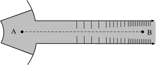
Figure 18. Illustration of the R-component $\Omega_{0}$ and the placement of the points $A$ and $B$.

Figure 19. We will estimate $\rho_{\Omega_{0}}(B,E)$ up to an additive factor by breaking it into three pieces: $[BC]$ is estimated by Lemma 12.2, $[DE]$ is estimated by Lemma 12.4, and $[CD]$ has bounded hyperbolic length by Lemma 12.3.

Lemma 12.2.

$\rho_{\Omega_{0}}(B,C)=\frac{1}{2}\log\frac{1}{|I|}+O(1)$.

Proof.

By Corollary 7.2, there is a disk $D_{n}$ so that $\{B,C\}\subset D_{n}\subset\Omega_{0}$, with $\operatorname{dist}(B,\partial D_{n})\simeq 1$ and $\operatorname{dist}(C,\partial D_{n})\simeq|I|$. Thus, $\rho_{\Omega_{0}}(B,C)\leq\rho_{D_{n}}(B,C)=\frac{1}{2}\log\frac{1}{|I|}+O(1).$

To prove the other direction, consider the arc on $\partial B_{n}$ given by Corollary 7.2. Let $\{z_{j}\}$ be the points where this arc intersects the vertical slits in $\partial\Omega_{0}$ and let $U=\mathbb{C}\setminus\{z_{j}\}$. Then $\Omega_{0}\subset U$, so $\rho_{\Omega_{0}}(B,C)\geq\rho_{U}(B,C)$. The points $\{z_{j}\}$ are about $|I|$ apart and there are $m\simeq 1/|I|$ such points. We can use a Möbius transformation to map $B_{n}$ to the upper half-plane, and so that $B$ and $C$ map to points at height $\simeq 1$ and $\simeq|I|$, respectively. The distance between the $\{z_{j}\}$ is distorted, but only boundedly, so the gaps are still $\simeq|I|$. By Lemma 11.1 and conformal invariance of hyperbolic distances, we deduce

$$\rho_{\Omega_{0}}(B,C)\geq\rho_{U}(B,C)\geq\frac{1}{2}\log\frac{1}{|I|}+O(1).\qed$$

Lemma 12.3.

With notation as above, $\rho_{\Omega_{0}}(C,D)=O(1)$.

Proof.

This is immediate from Koebe’s estimate, since $C$ and $D$ are connected by a segment in $\Omega_{0}$ whose Euclidean length is comparable to its distance from $\partial\Omega_{0}$. ∎

Lemma 12.4.

$\rho_{\Omega_{0}}(D,E)=\frac{\pi}{2}\frac{|J|}{|I|}+O(1).$

Proof.

This is immediate from Lemma 10.1. ∎

Lemma 12.5.

Let $\gamma$ denote the hyperbolic geodesic from $B$ to $E$ in the R-component. Then $\rho_{\Omega_{0}}(\gamma,D)=O(1)$ and $\rho_{\Omega_{0}}(\gamma,C)=O(1)$.

Proof.

The claim for $D$ follows immediately from Lemma 9.4. For $C$ it follows from this and Lemma 12.3. ∎

Corollary 12.6.

With notation as above,

(12.1) $$\rho_{\Omega_{0}}(B,E)=\rho_{\Omega_{0}}(B,C)+\rho_{\Omega_{0}}(C,D)+\rho_{\Omega_{0}}(D,E)+O(1)$$

Proof.

Using the triangle inequality, we immediately get “$\leq$”. To obtain the opposite inequality, let $\gamma$ be the hyperbolic geodesic in $\Omega_{0}$ connecting $B$ and $E$ and let $z_{C}$, $z_{D}$ be the points on $\gamma$ closest to $C$ and $D$ respectively. Then by Lemmas 12.5 and 12.3

$$\rho_{\Omega_{0}}(B,E) = \rho_{\Omega_{0}}(B,z_{C})+\rho_{\Omega_{0}}(z_{D},E)+\rho_{\Omega_{0}}(z_{C},z_{D})$$

$$\geq \rho_{\Omega_{0}}(B,C)-\rho_{\Omega_{0}}(C,z_{C})+\rho_{\Omega_{0}}(D,E)-\rho_{\Omega_{0}}(D,z_{D})$$

$$\qquad+\rho_{\Omega_{0}}(z_{C},C)+\rho_{\Omega_{0}}(C,D)+\rho_{\Omega_{0}}(D,z_{D})$$

$$\geq \rho_{\Omega_{0}}(B,C)+\rho_{\Omega_{0}}(C,D)+\rho_{\Omega_{0}}(D,E)+O(1).\qed$$

Lemma 12.7.

With notation as above, $\rho_{\Omega_{0}}(A,B)=\rho_{\Omega_{0}}(B,E)+O(1)$ .

Proof.

By Corollary 12.6 it is enough to prove

$$\rho_{\Omega_{0}}(A,B)=\rho_{\Omega_{0}}(B,C)+\rho_{\Omega_{0}}(C,D)+\rho_{\Omega_{0}}(D,E)+O(1).$$

Note that $B=\operatorname{Re}z_{0}+N+t_{n}+\frac{1}{2}\Delta_{n}$ for some $n$, $A=\operatorname{Re}z_{0}+N+2$, and by Lemmas 12.1 and 5.1

$$\rho_{\Omega_{0}}(A,B)=\frac{\pi}{2}(B-A)+O(1)=\frac{\pi}{2}t_{n}+O(1).$$

But by Lemmas 12.2, 12.3, 12.4, and 5.1, we have

$$\rho_{\Omega_{0}}(B,C)+\rho_{\Omega_{0}}(C,D)+\rho_{\Omega_{0}}(D,E) = \frac{1}{2}\log\frac{1}{|I|}+\frac{\pi}{2}\frac{|J|}{|I|}+O(1)$$

$$= -\frac{1}{2}\log\Delta_{n}+\frac{\pi}{2}\frac{y_{n+1}}{\Delta_{n}}+O(1).$$

Since $y_{n+1}=y_{n}+O(1)$, we get

$$\rho_{\Omega_{0}}(B,C)+\rho_{\Omega_{0}}(C,D)+\rho_{\Omega_{0}}(D,E)$$

$$\qquad\qquad=-\frac{1}{2}\log\Delta_{n}+\frac{\pi}{2}\frac{\Delta_{n}\left(t_{n}+\frac{1}{\pi}\log\Delta_{n}+O(1)\right)}{\Delta_{n}}+O(1)$$

$$\qquad\qquad=\frac{\pi}{2}t_{n}+O(1).\qed$$

We defined $\{y_{n}\}$ as we did so that (6.2) would hold, knowing that it would lead to Corollary 12.7, and thus to:

Lemma 12.8.

The $\tau$-lengths for $T$ are all comparable to $1$.

Proof.

Because of Lemma 12.7 and Lemma 9.3, the edges of the R-component shared with a neighboring L-component all have $\tau$-sizes comparable to $1$ (the $\tau$-lengths for the L-component are equal to $1$ by definition).

Next, we will show the same is true for the edges on the vertical slits. Consider a vertical tower $R$ of width $\Delta_{n}$ in the modified R-component between two adjacent vertical slits, see Figure 20. Divide the tower into squares as shown. Let $v_{k}$ be the center of the $k$-th square. By Lemma 10.1 the hyperbolic distance between $v_{1}$ and $v_{k}$ is $\frac{\pi}{2}k+O(1)$. Therefore, the image points in the right half-plane are the same hyperbolic distance apart. We verified above that the image of the first square is $\simeq 1$, so the $k$-th square has image with diameter $\simeq\exp(k\pi)$.

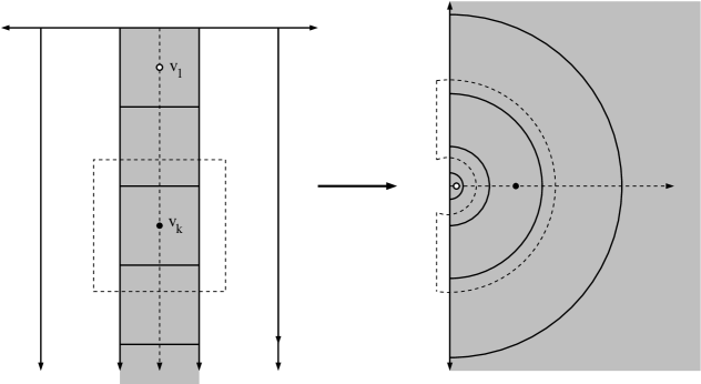
Figure 20. Each tower is divided into squares, whose $\tau$-images are approximate half-annuli whose Euclidean diameters grow exponentially. In particular, the $\tau$-lengths of the squares grow exponentially.

Moreover, for each $k\geq 2$, the $k$-th square can be expanded by a factor of $3/2$ (dashed box in Figure 20) and the conformal map $\tau$ can be extended to this larger box by reflection. Thus, by Koebe’s estimate $|\tau^{\prime}|\simeq\exp(\pi k)/\Delta_{n}$ uniformly on the $k$-th square. Since the side lengths of $T$ inside the $k$-th square are $\simeq\Delta_{n}\exp(-\pi k)$ by construction, they all have $\tau$-lengths $\simeq 1$.

A slightly different argument is needed for vertices on the last segment of each vertical slit (the one near the tip), that were defined using a square root map. This was done precisely so that $\tau$ would map these edges of $T$ to intervals on $\partial\mathbb{H}_{r}$ that have comparable lengths to each other, and the argument above shows these lengths are all $\simeq 1$. ∎

We have proven uniform lower and upper bounds for the $\tau$-sizes of all edges. By replacing $\tau$ by $c\cdot\tau$ for some $c>0$, if necessary, we may assume every $\tau$-length is at least $\pi$ and at most $O(1)$. The previous lemma, Lemma 3.3 and Lemma 8.2 imply:

Corollary 12.9.

With $T$, $\tau$ and $r$ as above, there is a $M<\infty$ (independent of $N$) so that $\tau(T(2r))\subset\{x+iy:0<x\leq M\}$.

13. $T(r)$ has finite area

The $\tau$-length bounds derived above give good control of the model function $F$. We now start to control the quasiconformal correction map $\varphi$. Recall that $T(r)$ is an open neighborhood of the tree $T$ defined in Section 3. Since $\varphi$ is conformal off $T(r)$, its dilatation $\mu$ is supported on $T(r)$, and we will prove this set is “small”. We begin by showing it has finite area.

Lemma 13.1.

Let $n\geq 2$ and consider the tower attached to the edge of length $\Delta_{n}$. Let $\{J_{k}\}$ be the collection of edges on the vertical sides of the tower. Then there exists a constant $C>0$, independent of $N$ and $n$, so that for any $0<\delta\leq 1$ we have

$$\sum_{k}(\operatorname{diam}J_{k})^{1+\delta}\leq\frac{C}{\delta}\cdot\Delta_{n}^{1+\delta}.$$

Proof.

In the construction, we subdivided the $n$-th “branch” into $m_{n}=\lfloor y_{n}/\Delta_{n}\rfloor$ many subintervals $\{J_{k}\}$. All but one of these (the “tip”) has length $\Delta_{n}$; consider these first. The $k$-th one is divided into $\simeq\exp(\pi k)$ smaller edges $\{J_{j,k}\}$ of equal length $\simeq\Delta_{n}\exp(-\pi k)$. Summing over these gives

$$\sum_{j,k}(\operatorname{diam}J_{j,k})^{1+\delta} \leq \sum_{k=1}^{m_{n}-1}\exp(\pi k)(\Delta_{n}\exp(-\pi k))^{1+\delta}$$

$$\leq \Delta_{n}^{1+\delta}\cdot\sum_{k=0}^{\infty}\exp(-\pi k\delta)$$

$$= \Delta_{n}^{1+\delta}\cdot O\left(\frac{1}{\delta}\right).$$

The last interval (i.e., the “tip”) has length $\leq 2\Delta_{n}$ and is divided into $\simeq\exp(\pi m_{n})$ intervals $J_{k}$, the longest of which has length $\simeq\Delta_{n}\exp(-\pi m_{n}/2)$. Thus

$$\sum\operatorname{diam}(J_{k})^{1+\delta} \leq (\Delta_{n}\exp(-\pi m_{n}/2))^{\delta}\sum\operatorname{diam}(J_{k})$$

$$\leq (\Delta_{n}\exp(-\pi m_{n}/2))^{\delta}(2\Delta_{n})$$

$$\leq 2\cdot\Delta_{n}^{1+\delta}.$$

Combining both cases we get the lemma. ∎

Lemma 13.2.

For each $R$-component $\Omega$, the Lebesgue area of $\Omega\cap T(r)$ is finite with a bound independent of $N$.

Proof.

The part of $T(r)$ outside the towers is easy to bound. Consider what happens in each tower with base $I_{k}$, which has length $\Delta_{k}$. The points of $T(r)$ in the $k$-th tower that are between distance $j\Delta_{k}$ and $(j+1)\Delta_{k}$ from the $L$-component are within $O(r\Delta_{k}\exp(-j))$ of a vertical side of the tower. Thus, the part of $T(r)$ inside this part of the tower has area bounded by $O(r\Delta_{k}^{2}\exp(-j))$. Summing over $j$ shows the total area of $T(r)$ within each tower is $O(r\Delta_{k}^{2})$. By Corollary 5.2 we have $\sum_{k}\Delta_{k}^{2}<\infty$, so the lemma follows, see Figure 21. ∎

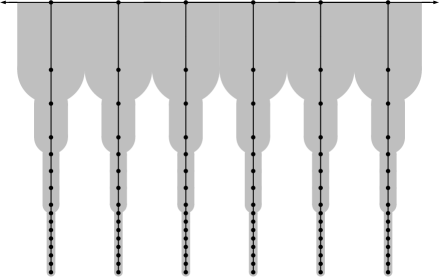
Figure 21. The neighborhood $T(r)$ narrows exponentially in each tower as we move away from the $L$-component, so the total area of $T(r)$ in each R-component is finite (and bounded independent of $N$).

It follows that the total area of $T(r)$ is $O(N)$.

14. Logarithmic area estimates for $T(r)$

The logarithmic area of a planar set $E$ with respect to a point $w$ is

$$\int_{E}\frac{dxdy}{|z-w|^{2}}.$$

We will show the logarithmic area of $T(r)$ is uniformly bounded for any base point outside $T(2r)$. This will give a bi-Lipschitz estimate on $\varphi$ in the next section.

Lemma 14.1.

Suppose $r>0$ and suppose $w\in\Omega\setminus T(2r)$. Then

$$\int_{T(r)}\frac{dxdy}{|w-z|^{2}}<C<\infty,$$

where $C$ is independent of $w$ and $N$.

Proof.

Let $r_{0}=\operatorname{dist}(w,\partial T(2r))$ and $D=D(w,r_{0})$. Let $r_{n}=r_{0}2^{n}$ and set $A_{n}(w)=\{z~{}:~{}r_{n-1}\leq|z-w|\leq r_{n}\}$ (we will drop the $w$ when the center of the annulus is clear from context). Note that $T(r)=\bigcup_{n=1}^{\infty}T(r)\cap A_{n}$. Furthermore, for $z\in A_{n}$ we have $|w-z|^{2}\geq r_{n-1}^{2}\simeq\operatorname{area}(A_{n})$. Thus it suffices to show

(14.1) $$\sum_{n=1}^{\infty}\frac{\operatorname{area}(T(r)\cap A_{n})}{\operatorname{area}(A_{n})}<\infty,$$

with a bound that is independent of $w$ and $N$. Note that each term in the series is bounded by $1$. First assume that $w$ is located in one of the “towers” along the horizontal edges of the R-component $\Omega$ (the remaining case will be dealt with later). Suppose this tower has top edge $I$ (the edge shared with a the adjacent L-component) and shorter vertical side $J$. It is convenient to break the sum into four parts:

1. $r_{n}<|I|$,

2. $|I|\leq r_{n}<|J|$,

3. $|J|\leq r_{n}<1$,

4. $1\leq r_{n}<\infty$.

In each case, the series will be dominated by a geometric series, whose sum is dominated by its largest term, and this will be $O(1)$ in every case.

Case 1 ($r_{n}<|I|$): See Figure 22. Suppose $w$ is distance $y$ from the top of the tower. The annulus $A_{n}$ hits at most one of the vertical segments in $\partial\Omega$ and this intersection is contained in a rectangle of height $O(r_{n})$ and width $O\left(re^{-y/|I|}\right)$, and thus has area at most $O\left(r_{n}re^{-y/|I|}\right)$. Also, since $D$ is outside $T(2r)$, if $A_{n}$ intersects $T(r)$ then $r_{n}$ must be at least comparable to $re^{-y/|I|}$. Thus, the non-zero terms of the sum satisfy

$$\frac{\operatorname{area}(T(r)\cap A_{n})}{\operatorname{area}(A_{n})}\leq O\left(\frac{r_{n}re^{-y/|I|}}{r_{n}^{2}}\right)=O\left(\frac{re^{-y/|I|}}{r_{n}}\right).$$

These form a decreasing geometric series whose largest term is $O(1)$. Thus the sum over Case 1 annuli is bounded by a constant independent of $w$ and $N$.

Figure 22. Case 1: annuli hit at most one vertical segment.

Case 2 ($|I|\leq r_{n}<|J|$): Consider horizontal strips of width $|I|$ as shown in Figure 23, and number them $k=1,\dots,m\simeq|J|/|I|$ starting from the top side of $\Omega$ and going down (this is assuming we are working near the top edge of $\Omega$; an identical argument works along the bottom edge). Recall that the interval of length $|I|$ which is $k|I|$ from the top edge was subdivided into $\exp(\pi k)$ pieces. By Lemma 12.8, the $\tau$-lengths of all these pieces are comparable to $1$. We thus obtain that in the $k^{\text{th}}$ strip $S_{k}$ the width of $T(r)$ around each vertical segment in $\partial\Omega$ is $O\left(\exp(-\pi k)\right)$. The area of $T(r)$ in each annulus is bounded by the area in the concentric axis-parallel square, whose side lengths equal the outer diameter of the annulus. In each such square $Q$, the area of $T(r)\cap Q\cap S_{k}$ decays geometrically with $k$ and hence is bounded by a multiple of the area in the top strip. Thus,

$$\frac{\operatorname{area}(T(r)\cap A_{n})}{\operatorname{area}(A_{n})}\leq Me^{-\pi k}$$

where $k$ is the smallest index such that $A_{n}$ hits the strip $S_{k}$. Since $r_{n}\geq|I|$, this index strictly decreases each time we increment $n$ and hence summing over all $n$ in this case gives a sub-sum of a geometric sum whose largest term (corresponding to $k=1$) is $O(1)$. Thus, the Case 2 terms sum to $O(1)$ with a uniform constant.

Figure 23. Case 2: Annuli hit two vertical segments, but not the neighboring L-component.

Case 3 ($|J|\leq r_{n}<1$): As in Case 2, we overestimate the area of $T(r)\cap A_{n}$ by replacing the annulus by a square $Q$, and estimating the area of $T(r)\cap Q$ by considering the horizontal strips $\{S_{k}\}$. See Figure 24. Note that annuli in this case have diameters that are at least comparable to $|I|$ (if $w\in S_{1}$, the “top” strip, defined in Case 2, then this is true since $w\not\in T(2r)$, and otherwise the annulus must be large enough to touch the neighboring L-component, and hence has diameter at least $|I|$). As before, the area is dominated by a multiple of the area of $Q\cap S_{1}$, which is bounded by a multiple of $|I|\operatorname{diam}(Q)$ (there are approximately $\operatorname{diam}(Q)/|I|$ towers hitting the annulus and each contributes area approximately $|I|^{2}$). Thus

$$\frac{\operatorname{area}(T(r)\cap A_{n})}{\operatorname{area}(A_{n})}\leq\frac{M|I|\operatorname{diam}(Q)}{r_{n}^{2}}=O\left(\frac{|I|}{r_{n}}\right)$$

In this case, $r_{n}$ starts by being at least as large as $|J|\geq|I|$ (and possibly much larger), and doubles at each step, so the terms of this sub-series are geometrically decaying. Thus, the sum is bounded by its first term, which is at most $O(1)$ with constants again being independent of $w$ and $N$.

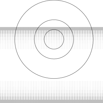
Figure 24. Case 3: annuli hit one, but not two, neighboring L-components.

Case 4 ($1\leq r_{n}<\infty$): By Lemma 13.2, $\Omega\cap T(r)$ has area $O(1)$, independent of $N$, for each $R$-component $\Omega$. Because of the way the R-components are arranged in the plane, a disk of radius $r_{0}$ can hit at most $O(r_{0})$ of them. Thus the annulus $A_{n}$ can intersect at most $O(r_{n})$ different $R$-components, so $\operatorname{area}(A_{n}\cap T(r))=O(r_{n})$. Since $\operatorname{area}(A_{n})\simeq r_{n}^{2}$, the ratio of these areas is $O(1/r_{n})$. Since $r_{n}$ increases geometrically, the Case 4 terms are bounded above by a geometrically decreasing series with first term of size $O(1)$, see Figure 25. Thus the sum over this case is also $O(1)$.

Figure 25. Case 4: Annuli with diameters $r_{n}\geq 1$ can hit at most $\max(N,O(r_{n}))$ different $R$-components, each contributing area at most $O(1)$. Thus the Case 4 terms are bounded by decreasing geometric series with largest term $O(1)$.

The four cases given above describe the proof of the lemma when the point $w$ is in one of the towers. If $w$ is not in a tower, but is in the region between the towers and the real axis, then a similar proof by enumerating cases will work. However, it is probably easier to argue as follows. For a $w$ that is not in a tower, choose $k$ so that $A_{k}$ is the smallest annulus of the form $A_{j}(w)$ that hits $T(r)$. Then it is easy to check that $A_{k+m}(w)$ contains a point $z$ in a tower and outside $T(2r)$ for some number $m$ that is independent of $w$. Let $s_{0}=\operatorname{dist}(z,\partial T(2r))$ and $s_{l}=s^{l}s_{0}$. Let $n>k+m+2$. Then there exists some $l$ so that $r_{n}\leq s_{l}<r_{n+1}$. We then have

$$A_{n}(w)\subset A_{l-2}(z)\cup A_{l-1}(z)\cup A_{l}(z)\cup A_{l+1}(z).$$

Thus, the series (14.1) for $w$ is bounded above by $O(1)$ terms, each bounded by $1$, plus four times the corresponding series for $z$. By our previous argument, the latter is uniformly bounded and hence so is the series for $w$. ∎

15. A bi-Lipschitz estimate for the correction map

Recall from the statement of Theorem 3.4 that our entire function is of the form $f=\sigma\circ\tau\circ\varphi^{-1}$. Thus inside the R-components, we have $f^{-1}=\varphi\circ\tau^{-1}\circ\log$. The logarithm is easy to understand, the map $\tau^{-1}$ is conformal on a half-plane and the estimates we need for it are all well known. Only the quasiconformal map $\varphi$ holds some mystery, but we will show that it is completely harmless, at least for estimating dimension, because it is bi-Lipschitz with a uniform constant near the Julia set (however, it need not be bi-Lipschitz everywhere in $\mathbb{C}$).

Lemma 15.1.

Suppose $A,B$ are disjoint, planar sets and

$$\int_{A}\frac{dxdy}{|z-w|^{2}}\leq C<\infty,$$

for all $w\in B$. If $\varphi$ is a $K$-quasiconformal map that is conformal off $A$, then $\varphi$ is $M$-bi-Lipschitz on $B$ with $M$ depending only on $C$ and $K$, i.e., for all $w,z\in B$,

$$0<\frac{1}{M(C,K)}\leq\frac{|\varphi(z)-\varphi(w)|}{|z-w|}\leq M(C,K)<\infty.$$

Proof.

This is more-or-less immediate from results of Bojarski, Lehto, Teichmüller and Wittich [7], [26], [40], [42] although we shall give specific references to the more recent paper [9] which also gives the higher dimensional versions of the two dimensional results we will use.

First we prove that $\varphi$ is asymptotically conformal at $\infty$. Let $w\in B$. Denote by $\mu(z)$ the dilatation of $\varphi$. This function is supported on $A$. Thus, we get

$$\int_{|z|>|w|}\frac{|\mu(z)|dxdy}{|z|^{2}}\leq\int_{A\cap\{|z|>|w|\}}\frac{dxdy}{|z|^{2}}\leq\int_{A}\frac{4dxdy}{|z-w|^{2}}\leq 4C.$$

Hence, (see for example [26, Chapter V, Theorem 6.1]) there is a $c\neq 0$ so that

$$\lim_{z\to\infty}\frac{\varphi(z)}{z}=c.$$

Now suppose $z,w\in B$ and let $r=|z-w|$. Note that

$$\{\xi:|\xi-z|=R\}\subset\{\xi:R-|z|\leq|\xi|\leq R+|z|\}.$$

If $R$ is large enough, $\varphi$ maps the round annulus $A(z,r,R)=\{\xi:r<|\xi-z|<R\}$ to a topological annulus $A^{\prime}$ whose outer boundary is contained in the annulus $A(\varphi(z),|c|R/2,2|c|R)$ and whose inner boundary is a closed Jordan curve $\gamma$. By taking $R$ large enough, we can assume $\gamma$ hits the disk $D(\varphi(z),|c|R/4)$. Therefore,

$$\mathrm{mod}(A^{\prime})=\mathrm{mod}(A(\varphi(z),\operatorname{diam}(\gamma),R))+O(1)=\log R-\log\operatorname{diam}(\gamma)+O(1).$$

On the other hand, Corollary 2.10 of [9] says that

$$\mathrm{mod}(A^{\prime}) =\mathrm{mod}(A(z,r,R))+O\left(\int_{r<|\xi-z|<R}\frac{|\mu(\xi)|}{|\xi|^{2}}dxdy\right)$$

$$=\mathrm{mod}(A(z,r,R))+O\left(\int_{A\cap\{r<|\xi-z|<R\}}\frac{1}{|\xi|^{2}}dxdy\right)$$

$$=\log R-\log r+O(1).$$

Thus, $\log\operatorname{diam}(\gamma)=\log r+O(1)$, or $\operatorname{diam}(\gamma)\simeq r$. Since $\varphi$ is quasiconformal, the segment $S$ connecting $z$ and $w$ maps to a quasi-arc and hence satisfies the Ahlfors three-point condition (e.g., Theorem II.8.6 of [26]), so $|\varphi(z)-\varphi(w)|\simeq\operatorname{diam}(\varphi(S))$. Since quasiconformal maps are quasisymmetric $\operatorname{diam}(\varphi(S))\simeq\operatorname{diam}(\gamma)$ (first due to Gehring [21]; see also Section 4 of [23]). Thus, $|\varphi(z)-\varphi(w)|\simeq|z-w|,$ as desired. ∎

Lemma 15.2.

The correction map $\varphi$ is bi-Lipschitz on $\mathbb{C}\setminus T(2r)$, that is, there exists a constant $M>0$ (independent of $N$) such that

$$\frac{1}{M}\leq\frac{|\varphi(z)-\varphi(w)|}{|z-w|}\leq M$$

for all $z,w\in\mathbb{C}\setminus T(2r)$.

Proof.

Define $A=T(r)$ and $B=\mathbb{C}\setminus T(2r)$. Let $w\in B$. By Lemma 14.1, there exists some $C>0$, independent of $N$ and $w$, so that

$$\int_{A}\frac{dxdy}{|z-w|^{2}}<C<\infty.$$

Applying Lemma 15.1 proves this lemma. ∎

16. Proof of (1.1): the initial covering exists

We have now completed the preliminary estimates. In the next two sections we finish the proof of Theorem 1.1 by establishing (1.1) and (1.2) from the introduction. One of the main facts we need is the following result.

Lemma 16.1.

Let $\Omega\neq\mathbb{C}$ be simply connected and let $\tau:\Omega\to\mathbb{H}_{r}$ be conformal. Let $z=x+iy$ with $x>1$ and let $V\subset\mathbb{H}_{r}$ be a simply connected neigbourhood of $z$ with hyperbolic radius bounded by $r$. If $w=\tau^{-1}(1+iy)$ and $U=\tau^{-1}(V)$, then we have

$$\operatorname{diam}(U)=O(|\tau^{\prime}(w)|^{-1}x\operatorname{diam}(V))$$

where the constant depends only on $r$ and the diameter is the Euclidean diameter.

Proof.

The distortion theorem for conformal maps (e.g., Theorem I.4.5 of [20]) says that if $\psi:\mathbb{D}\to\Omega$ is conformal, then

(16.1) $$|\psi^{\prime}(z)|\leq|\psi^{\prime}(0)|\frac{1+|z|}{(1-|z|)^{3}}\leq|\psi^{\prime}(0)|\frac{2}{(1-|z|)^{3}}.$$

Moreover, the derivative of a conformal map has comparable absolute values at any two points of a compact set, with a constant that depends only on the hyperbolic diameter of the set. Thus for any compact $K$ in the disk $\mathbb{D}$,

$$\operatorname{diam}(\psi(K))=O(\operatorname{diam}(K)|\psi^{\prime}(z)|),$$

where these are Euclidean diameters and where $z$ is any point of $K$. The constant depends only on the hyperbolic diameter of $K$ and not on $z$ or $\psi$.

If $\Psi$ is a conformal map from the right half-plane $\mathbb{H}_{r}$ to $\Omega$, then we can write it as a composition of the Möbius transformation $\sigma(z)=(z-1)/(z+1)$ from the half-plane to the disk, followed by a conformal map $\psi$ from the disk to $\Omega$. Note that $\sigma(1)=0$, $\sigma(\infty)=1$, and $|\sigma^{\prime}(x)|=2/(x+1)^{2}\leq 2/x^{2}$ for $x\in[1,\infty)$. Also note that $1-\sigma(x)=\frac{2}{x+1}\geq 1/x$ for $x\geq 1$. Using (16.1), these observations, and the chain rule, we deduce that

$$|\Psi^{\prime}(x)| = |\psi^{\prime}(\sigma(x))|\cdot|\sigma^{\prime}(x)|$$

$$\leq |\psi^{\prime}(0)|\frac{2}{(1-|\sigma(x)|)^{3}}\cdot\frac{2}{x^{2}}$$

$$\leq 4\frac{|\Psi^{\prime}(1)|}{|\sigma^{\prime}(1)|}\frac{x^{3}}{x^{2}}$$

$$= 8|\Psi^{\prime}(1)|x,$$

for $x\geq 1$. By considering a vertical translate $\tilde{\Psi}(z)=\Psi(z+iy)$ of $\Psi$ and applying the arguments above to $\tilde{\Psi}$ we see that

$$|\Psi^{\prime}(x+iy)|=O(|\Psi^{\prime}(1+iy)|\cdot x),$$

for $x\geq 1$. The lemma follows by applying this discussion to $\Psi=\tau^{-1}$. ∎

Lemma 16.2.

If $N$ is large enough, then the Julia set for $f$ is contained in the union of $N$ bounded width strips passing through the origin. More precisely, there are a $C,M<\infty$ (independent of $N$) so that

$$\mathcal{J}(f)\subset\{z\in\mathbb{C}:|z|>N/(2C),\,\operatorname{dist}(z,X)\leq M\}$$

where $X=\{w:w^{N}\in\mathbb{R}\}$.

Proof.

Our entire functions are of the form $f=g\circ\varphi^{-1}$ where $g$ is quasiregular and $\varphi$ is a quasiconformal homeomorphism of the plane. Both $g$ and $\varphi$ were chosen to fix the origin and $g$ maps the disk $D(0,N)$ into the unit disk. Lemma 15.2 shows that $\varphi$ is bi-Lipschitz with some constant $C<\infty$ in $D(0,N/2)$, since this disk is contained inside the central D-component but outside $T(2r)$, if $N$ is large enough. Thus $\varphi^{-1}$ maps $D(0,N/(2C))$ into $D(0,N/2)$. Hence $f$ maps $D(0,N/(2C))$ into the unit disk, and hence into itself for $N$ large enough. Therefore, $D=D(0,N/(2C))$ is inside the Fatou set of $f$. In particular,

$$\mathcal{J}(f)\subset\{z:|f(z)|>N/(2C)\})\subset\varphi(\{z:|g(z)|>N/(2C)\}).$$

If $N>2C$, then by construction $\{z:|g(z)|>N/(2C)\}\subset\{z:|g(z)|>1\}$ lies in the union of R-components. In particular, $|g(z)|\leq 1$ for all points outside the R-components. Also by construction, $g$ maps $X$ to itself and the union of R-components is contained in a unit neighborhood of $X\setminus D(0,N)$. Moreover, we claim that $\varphi$ fixes each arm of the set $X$.

One way to verify this is to construct $\varphi$ as follows. Use the measurable Riemann mapping theorem to find a quasiconformal map from the sector $\{w:|\arg(w)|<\pi/2N\}$ with the same dilatation and fixing $0$ and $\infty$; then extend the map to the whole plane by reflecting across the arms of $X$ one at a time. We end with a quasiconformal map of the plane and the correct dilatation, so it must be $\varphi$ (up to a positive dilation). Moreover, it preserves the arms of $X$ by its definition, proving the claim.

Since $\varphi$ preserves the arms of $X$ and it is $C$-bi-Lipschitz on the part of the arms of $X$ that lie outside $T(2r)$ (this is all but a bounded segment), and since it is quasisymmetric on the whole plane, there is a $M<\infty$ so that

$$\varphi(\{z:\operatorname{dist}(z,X)\leq 1\})\subset\{z:\operatorname{dist}(z,X)\leq M\}).$$

In particular

$$\mathcal{J}(f) \subset \varphi(\{z:|g(z)|>1\})$$

$$\subset \varphi(\{z:|z|>N/2,\operatorname{dist}(z,X)\leq 1\})$$

$$\subset \{z:|z|>N/(2C),\operatorname{dist}(z,X)\leq M\}.\qed$$

Proof of (1.1).

The Julia set is contained in the union of $2N$ half-strips of fixed width $M$. Due to the symmetries in the construction, it will suffice to consider coverings of only one of these, say $S_{0}$, the half-strip intersecting the positive real axis. This half-strip can be covered by a collection squares $\{Q_{n}\}$ of side length $M$ and centered at points $n=\{\lfloor N/(2M)\rfloor,1+\lfloor N/(2M)\rfloor,\dots\}$. Obviously, the diameters of these squares are all about unit size, hence they are not summable. However, we shall show that given $\delta>0$, we can choose $N$ large enough so that

$$\sum\operatorname{diam}(f^{-1}(Q_{n}))^{1+\delta}<\infty,$$

where the sum is over all preimages outside $D(0,r_{N})$ (we need only consider preimages hitting the Julia set and this disk is in the Fatou set).

Note that $f^{-1}=\varphi\circ g^{-1}$. There are $2N$ R-components, and preimages under $g$ can lie in any of these, but for the moment we only consider $g$-preimages in the R-component that intersects the positive real axis. Off the set $T(r)$, $g(z)=\exp(\tau(z))$ where $\tau:\Omega_{0}\to\mathbb{H}_{r}$ is conformal. Therefore, $g^{-1}(Q)$ for $Q\subset\mathbb{H}_{r}\setminus\tau(T(r))$, is given by first taking inverse images under the exponential map, then under the conformal map $\tau$. Both are easy to understand.

The inverse image of $Q_{n}$ under $e^{z}$ is a countable union of sets of diameter $O(1/n)$. The sets are all vertical translates of each other and there is exactly one containing each point of the form $z_{n,k}=\log n+k2\pi i$. Suppose $Y_{n,k}$ is the preimage of $Q_{n}$ containing $z_{n,k}$. Let $P_{n,k}=\tau^{-1}(Y_{n,k})$, and $w_{k}=\tau^{-1}(1+2\pi ki)$.

Lemma 16.3.

$\operatorname{diam}(P_{n,k})=O(|\tau^{\prime}(w_{k})|^{-1}\cdot\frac{\log n}{n})$.

Proof.

This follows immediately from Lemma 16.1, since $Y_{n,k}$ has diameter $O(1/n)$ and hits the vertical line $\{x=\log n\}$. ∎

Each of the points $z_{n,k}$ is associated, by horizontal projection, to one of the intervals $[2\pi ni,2\pi(n+1)i]$ on $\partial\mathbb{H}_{r}$ and each point $w_{n,k}$ is associated to an edge of the folded graph $T^{\prime}$. Each edge of $T^{\prime}$ is associated to a side $I_{k}$ of the R-component and at most $O(1)$ edges of $T^{\prime}$ correspond to any such side of the $R$-component (this is because the $\tau$-lengths of all sides are uniformly bounded). In particular, for any $0<\delta\leq 1$,

$$|\tau^{\prime}(w_{n,k})|\simeq\frac{1}{\operatorname{diam}(I_{k})},$$

$$\operatorname{diam}(P_{n,k})=O\left(\frac{\operatorname{diam}(I_{k})\log n}{n}\right),$$

$$\sum_{k}\sum_{n}\operatorname{diam}(P_{n,k})^{1+\delta}\leq C\left(\sum_{k}\operatorname{diam}(I_{k})^{1+\delta}\right)\left(\sum_{n}\left(\frac{\log n}{n}\right)^{1+\delta}\right).$$

The first term in the product is finite by construction (see Corollary 5.2 and Lemma 13.1) and the second is finite by a simple calculus exercise. Note that none of these bounds depend on $N$. This shows that the $g$-preimages of the $\{Q_{n}\}$ have diameters whose $(1+\delta)$-powers have a finite sum. Lemma 15.2 shows that the images of these preimages under the correction map have comparable diameters, so the same is true for the $f$-preimages, if the $g$-preimages lie outside $T(2r)$. But this is fulfilled if $N$ is large enough so that $r_{N}$ is larger than $\exp(2A)$ where $A$ is the upper bound on the $\tau$-sizes of the edges obtained in Lemma 12.8.

In the argument so far we have assumed we started with a covering $\{Q_{n}\}$ of one tract of $f$ and we only counted $g$-preimages that were in a single tract of $g$. Since $f$ and $g$ both have $2N$ tracts, the sum over all preimages of coverings of all tracts will be larger by a factor of $4N^{2}$, and this is clearly still finite. ∎

17. Proof of (1.2): the iterative step

Next, we will prove the iterative step which finishes the proof of Theorem 1.1.

Lemma 17.1.

Suppose $f=g\circ\varphi^{-1}$ is as above. Let $D=D(w,r)$ be a disk with $|w|>r_{N}+1$ and $r<1$ (so $D$ is disjoint from the closed disk $D(0,r_{N})$). Let $\{D_{j}\}$ be the connected components of $f^{-1}(D)$. Given $\epsilon>0$ and $\delta>0$, if $N$ is sufficiently large, then

$$\sum_{j}\operatorname{diam}(D_{j})^{1+\delta}\leq\epsilon\cdot\operatorname{diam}(D)^{1+\delta}.$$

Proof.

We can write the inverse of $f$ by taking a complex logarithm, followed by the conformal map of the right half-plane to an R-component, followed by the correction map $\varphi$. The correction map will only be applied to sets where it is bi-Lipschitz, so it only adds a uniformly bounded multiplicative factor to the sum in the lemma.

First, the logarithm of the disk $D$ is an infinite collection of disjoint sets of diameter $O(r/|w|)$ arranged on the vertical line $\{x=\log|w|\}$. By Corollary 12.9 we have

(17.1) $$\tau(T(2r))\subset V_{M}=\{x+iy:0<x\leq M\}.$$

If $N$ so large that $r_{N}>\exp(M)$, where $M$ is the $N$-independent upper bound for the $\tau$-sizes of the edges of the graph, we have

(17.2) $$\log|w|>\log r_{N}>M.$$

Each component contains one point of the form $\log|w|+i(\theta+2\pi k),$ where $\theta=\arg(w)$. By Equation (17.2), all these sets lie in a sub-half-plane

$$\mathbb{H}_{r}+M=\mathbb{H}_{r}\setminus V_{M}=\{x+iy:x>M\}.$$

By Lemma 16.1 the preimages have diameters bounded by

$$O\left(\left|\left(\tau^{-1}\right)^{\prime}\left(1+i\left(2\pi k+\theta\right)\right)\right|\frac{r\log|w|}{|w|}\right) =O\left(\operatorname{diam}(I_{k})\frac{r\log|w|}{|w|}\right).$$

Since $|w|\geq r_{N}>N$ and $x\mapsto\log(x)/x$ is decreasing for $x>e$, this is bounded by

$$O\left(\operatorname{diam}(I_{k})\frac{r\log|N|}{N}\right).$$

Sum over $k$, use Lemma 13.1 and Corollary 5.2, and recall that there are $2N$ $R$-components to consider:

$$\sum_{k}\left(\operatorname{diam}D_{k}\right)^{1+\delta}\leq\frac{C}{\delta}\cdot r^{1+\delta}\cdot\frac{(\log N)^{1+\delta}N}{N^{1+\delta}}\leq\frac{C}{\delta}\cdot r^{1+\delta}\cdot\frac{(\log N)^{1+\delta}}{N^{\delta}}.$$

Taking $N$ large enough gives the desired estimate for the quasiregular map $g$. By (17.2) and (17.1), the $g$-preimages of $D$ lie outside $T(2r)$. By Lemma 15.2, the correction map expands the diameters by a bounded factor (independent of $N$). Taking $N$ even larger, if necessary, proves the lemma. ∎

This completes the proof of Theorem 1.1: Speiser class Julia sets may have dimension as close to $1$ as desired.

Our examples have three singular values. Is it possible to build entire functions with only two singular values whose Julia sets have dimensions as close to $1$ as we wish? Does every dimension in $(1,2]$ occur for some $f\in\mathcal{S}$?

Two entire functions $f,g$ are said to be quasiconformally equivalent if there are quasiconformal homeomorphisms $\psi,\phi$ of the plane so that $f\circ\psi=\phi\circ g$. The set of functions QC-equivalent to a given Speiser class function $f$ forms a finite dimensional complex manifold $M_{f}$ (the complex dimension is $q+2$ where $q$ is the number of singular values; see Section 3 of [18]). Basic properties of quasiconformal maps imply that $\dim(\mathcal{J}(g))$ is a continuous function on $M_{f}$, and also imply that if this function attains the value $2$, then it is constant on $M_{f}$. Can it ever be non-constant? Probably this is common, but it is not even clear what happens for the examples constructed in this paper. Can the dimension ever be constant on $M_{f}$ with a value other than $2$? If not, is $\sup\{\dim(\mathcal{J}(g)):g\in M_{f}\}=2$ for every $f$?

18. The Julia set is a Cantor Bouquet

A Cantor bouquet is a closed set in the plane so that there is a homeomorphism of the plane mapping it to a “straight brush” in the sense of Aarts and Oversteegen, see [1]. This is a subset $B$ of $[0,\infty)\times(\mathbb{R}\setminus\mathbb{Q})$ that is closed in the plane and such that
(1) every point of $B$ is contained in a closed horizontal ray, called a hair,
(2) the horizontal projection of $B$ onto the $y$ axis is dense,
(3) any point of $B$ can be approached from above or below by endpoints of hairs.
Any two such sets are homeomorphic, and can even be mapped to each other by a homeomorphism of the plane (i.e., they are ambiently homeomorphic). See [1], [17].

Lemma 18.1.

The Julia sets of our examples are Cantor bouquets.

Proof.

The construction in this paper shows that our examples have the following properties: $0$ is an attracting fixed point and all three singular values ($0,-1,1$) are contained in the basin of attraction of $0$ (which contains a large disk around the origin). This means our maps are of disjoint type, i.e., the singular set is compact and contained in the immediate attracting basin of an attracting fixed point.

A tract of an entire function is a connected component of $\{z:|f(z)|>R\}$. These are unbounded Jordan domains. If a tract $\Omega$ of $f$ does not contain zero, then consider a connected component $\Omega^{\prime}$ of $\log(\Omega)$ for some branch of the logarithm (there are countably many such and any two are related by a vertical translate by an integer multiple of $2\pi$. We say that a curve $\gamma\subset\Omega^{\prime}$ from a point $z_{0}\in\overline{\Omega^{\prime}}$ to $\infty$ has bounded wiggling if there are real constants $A,B$ so that for any point $z\in\gamma$ we have $\operatorname{Re}(z)>A\cdot\operatorname{Re}(z_{0})-B.$ The domain $\Omega^{\prime}$ is said to have uniformly bounded wiggling if all the hyperbolic geodesics from $z_{0}\in\overline{\Omega^{\prime}}$ to $\infty$ have bounded wiggling (with uniform constants).

Proposition 5.4 of [34] implies that if $f$ is in the Eremenko-Lyubich class and the tracts of $f$ have uniformly bounded wiggling, then $f$ satisfied a condition called the “uniform linear head-start condition”. We won’t define this condition, but we note that Corollary 6.3 of [4] says that if an entire function is disjoint-type and has the uniform head-start condition, then the Julia set is a Cantor bouquet. Thus, [34] and [4] combined imply that disjoint-type plus bounded wiggling imply the Julia set is a Cantor bouquet. Hence, it suffices to show that our examples have bounded wiggling.

The logarithms of the $R$-components we construct in this paper clearly have this property. These components are mapped to the tracts of our entire functions by the correction map $\varphi$. Let $R$ be a tract of the quasiregular map $g$ and $S=\varphi(R)$ the corresponding tract of the entire function $f$. Let $R^{\prime}$ be a component of $\log(R)$ and $S^{\prime}$ a component of $\log(S)$. Choosing the correct branch of the logarithm, the map $h(z)=\log(\varphi(\exp(z)))$ maps $R^{\prime}$ conformally onto $S^{\prime}$. The estimates of this paper show that $\varphi$ is asymptotically conformal, i.e., there is a constant $c\neq 0$ so that

$$\left|\frac{\varphi(z)}{z}-c\right|=o(1)\quad\text{as}\quad|z|\to\infty$$

or in other words $\varphi(z)=cz+o(|z|)\quad\text{as}\quad|z|\to\infty.$ Hence,

$$\log(\varphi(z))=\log(z)+\log(c)+\log\left(1+o(1)\right)=\log(z)+O(1)$$

which yields $|h(z)-z|=O(1)$. This easily implies that hyperbolic geodesics in $R^{\prime}$ map to curves of bounded wiggling in $S^{\prime}$. This in turn implies the hyperbolic geodesics in $S^{\prime}$ have bounded wiggling by [34, Lemma A.2]. ∎

For disjoint-type, finite-order maps, Barański [3] proved that the Julia set is a Cantor bouquet whose endpoints have dimension 2 and the rest of the bouquet has dimension $1$ (this was proven earlier for exponential maps by Karpińska [24]). In our example, the non-endpoints are escaping (see Theorem 5.1 in [31]) and this should imply that they have dimension $1$, and so we expect that the dimension of the whole Julia set is concentrated on the endpoints, but we leave this for future investigation.

References

- [1] J. Aarts and L. Oversteegen. The geometry of Julia sets. Trans. Amer. Math. Soc., 338(2):897–918, 1993.
- [2] I. N. Baker. The domains of normality of an entire function. Ann. Acad. Sci. Fenn. Ser. A I Math., 1(2):277–283, 1975.
- [3] K. Barański. Hausdorff dimension of hairs and ends for entire maps of finite order. Math. Proc. Cambridge Philos. Soc., 145(3):719–737, 2008.
- [4] K. Barański, X. Jarque, and L. Rempe. Brushing the hairs of transcendental entire functions. Topology Appl., 159(8):2102–2114, 2012.
- [5] K. Barański, B. a. Karpińska, and A. Zdunik. Hyperbolic dimension of Julia sets of meromorphic maps with logarithmic tracts. Int. Math. Res. Not. IMRN, (4):615–624, 2009.
- [6] A. F. Beardon. The hyperbolic metric in a rectangle. II. Ann. Acad. Sci. Fenn. Math., 28(1):143–152, 2003.
- [7] P. P. Belinskii. Obshchie svoistva kvazikonformnykh otobrazhenii. Izdat. “Nauka” Sibirsk. Otdel., Novosibirsk, 1974.
- [8] W. Bergweiler, P. J. Rippon, and G. M. Stallard. Dynamics of meromorphic functions with direct or logarithmic singularities. Proc. Lond. Math. Soc. (3), 97(2):368–400, 2008.
- [9] C. Bishop, V. Y. Gutlyanskiĭ, O. Martio, and M. Vuorinen. On conformal dilatation in space. Int. J. Math. Math. Sci., (22):1397–1420, 2003.
- [10] C. Bishop and Y. Peres. Fractals in probability and analysis, volume 162 of Cambridge Studies in Advanced Mathematics. Cambridge University Press, Cambridge, 2017.
- [11] C. J. Bishop. Constructing entire functions by quasiconformal folding. Acta Math., 214(1):1–60, 2015.
- [12] C. J. Bishop. Models for the Eremenko-Lyubich class. J. Lond. Math. Soc. (2), 92(1):202–221, 2015.
- [13] C. J. Bishop. Models for the Speiser class. Proc. Lond. Math. Soc. (3), 114(5):765–797, 2017.
- [14] C. J. Bishop. A transcendental Julia set of dimension 1. Invent. Math., 212(2):407–460, 2018.
- [15] C. J. Bishop and K. Lazebnik. Prescribing the postsingular dynamics of meromorphic functions. Math. Ann., 375(3-4):1761–1782, 2019.
- [16] X. Buff and A. Chéritat. Quadratic Julia sets with positive area. Ann. of Math. (2), 176(2):673–746, 2012.
- [17] W. Bula and L. Oversteegen. A characterization of smooth Cantor bouquets. Proc. Amer. Math. Soc., 108(2):529–534, 1990.
- [18] A. È. Erëmenko and M. Y. Lyubich. Dynamical properties of some classes of entire functions. Ann. Inst. Fourier (Grenoble), 42(4):989–1020, 1992.
- [19] N. Fagella, S. Godillon, and X. Jarque. Wandering domains for composition of entire functions. J. Math. Anal. Appl., 429(1):478–496, 2015.
- [20] J. Garnett and D. Marshall. Harmonic measure, volume 2 of New Mathematical Monographs. Cambridge University Press, Cambridge, 2008. Reprint of the 2005 original.
- [21] F. W. Gehring. The definitions and exceptional sets for quasiconformal mappings. Ann. Acad. Sci. Fenn. Ser. A I No., 281:28, 1960.
- [22] L. Goldberg and L. Keen. A finiteness theorem for a dynamical class of entire functions. Ergodic Theory Dynam. Systems, 6(2):183–192, 1986.
- [23] J. Heinonen and P. Koskela. Quasiconformal maps in metric spaces with controlled geometry. Acta Math., 181(1):1–61, 1998.
- [24] B. Karpińska. Hausdorff dimension of the hairs without endpoints for . C. R. Acad. Sci. Paris Sér. I Math., 328(11):1039–1044, 1999.
- [25] K. Lazebnik. Several constructions in the Eremenko-Lyubich class. J. Math. Anal. Appl., 448(1):611–632, 2017.
- [26] O. Lehto and K. I. Virtanen. Quasiconformal mappings in the plane. Springer-Verlag, New York-Heidelberg, second edition, 1973. Translated from the German by K. W. Lucas, Die Grundlehren der mathematischen Wissenschaften, Band 126.
- [27] C. McMullen. Area and Hausdorff dimension of Julia sets of entire functions. Trans. Amer. Math. Soc., 300(1):329–342, 1987.
- [28] H. Mihaljević-Brandt and L. Rempe-Gillen. Absence of wandering domains for some real entire functions with bounded singular sets. Math. Ann., 357(4):1577–1604, 2013.
- [29] M. Misiurewicz. On iterates of . Ergodic Theory Dynamical Systems, 1(1):103–106, 1981.
- [30] J. W. Osborne and D. J. Sixsmith. On the set where the iterates of an entire function are neither escaping nor bounded. Ann. Acad. Sci. Fenn. Math., 41(2):561–578, 2016.
- [31] L. Rempe, P. J. Rippon, and G. M. Stallard. Are Devaney hairs fast escaping? J. Difference Equ. Appl., 16(5-6):739–762, 2010.
- [32] L. Rempe-Gillen. Arc-like continua, Julia sets of entire functions, and Eremenko’s Conjecture. ArXiv e-prints, Oct. 2016.
- [33] P. J. Rippon and G. M. Stallard. Dimensions of Julia sets of meromorphic functions with finitely many poles. Ergodic Theory Dynam. Systems, 26(2):525–538, 2006.
- [34] G. Rottenfusser, J. Rückert, L. Rempe, and D. Schleicher. Dynamic rays of bounded-type entire functions. Ann. of Math. (2), 173(1):77–125, 2011.
- [35] H. Schubert. Über die Hausdorff-Dimension der Juliamenge von Funktionen endlicher Ordnun. PhD thesis, Christian-Albrechts-Universität zu Kiel, 2007.
- [36] M. Shishikura. The Hausdorff dimension of the boundary of the Mandelbrot set and Julia sets. Ann. of Math. (2), 147(2):225–267, 1998.
- [37] G. Stallard. The Hausdorff dimension of Julia sets of entire functions. III. Math. Proc. Cambridge Philos. Soc., 122(2):223–244, 1997.
- [38] G. Stallard. The Hausdorff dimension of Julia sets of entire functions. IV. J. London Math. Soc. (2), 61(2):471–488, 2000.
- [39] G. Stallard. The Hausdorff dimension of Julia sets of hyperbolic meromorphic functions. II. Ergodic Theory Dynam. Systems, 20(3):895–910, 2000.
- [40] O. Teichmüller. Untersuchungen über konforme and quasikonforme Abbildung. Deutsche Math., 3:621–678, 1938.
- [41] J. Waterman. Wiman-Valiron disks and the dimension of Julia sets. 2019. Preprint, arXiv:1910.08474 [math.DS].
- [42] H. Wittich. Zum Beweis eines Satzes über Quasikonforme Abbildungen. Math. Z., 51:278–288, 1948.
- [43] M. Zinsmeister. Fleur de Leau-Fatou et dimension de Hausdorff. C. R. Acad. Sci. Paris Sér. I Math., 326(10):1227–1232, 1998.