Long-Tail Learning via Logit Adjustment

Abstract

Real-world classification problems typically exhibit an imbalanced or long-tailed label distribution, wherein many labels are associated with only a few samples. This poses a challenge for generalisation on such labels, and also makes naïve learning biased towards dominant labels. In this paper, we present two simple modifications of standard softmax cross-entropy training to cope with these challenges. Our techniques revisit the classic idea of logit adjustment based on the label frequencies, either applied post-hoc to a trained model, or enforced in the loss during training. Such adjustment encourages a large relative margin between logits of rare versus dominant labels. These techniques unify and generalise several recent proposals in the literature, while possessing firmer statistical grounding and empirical performance. A reference implementation of our methods is available at:

https://github.com/google-research/google-research/tree/master/logit_adjustment.

1 Introduction

Real-world classification problems typically exhibit a long-tailed label distribution, wherein most labels are associated with only a few samples (Van Horn and Perona, 2017; Buda et al., 2017; Liu et al., 2019). Owing to this paucity of samples, generalisation on such labels is challenging; moreover, naïve learning on such data is susceptible to an undesirable bias towards dominant labels. This problem has been widely studied in the literature on learning under class imbalance (Cardie and Howe, 1997; Chawla et al., 2002; Qiao and Liu, 2009; He and Garcia, 2009; Wallace et al., 2011) and the related problem of cost-sensitive learning (Elkan, 2001; Zadrozny and Elkan, 2001; Masnadi-Shirazi and Vasconcelos, 2010; Dmochowski et al., 2010).

Recently, long-tail learning has received renewed interest in the context of neural networks. Two active strands of work involve post-hoc normalisation of the classification weights (Zhang et al., 2019; Kim and Kim, 2019; Kang et al., 2020; Ye et al., 2020), and modification of the underlying loss to account for varying class penalties (Zhang et al., 2017; Cui et al., 2019; Cao et al., 2019; Tan et al., 2020). Each of these strands is intuitive, and has proven empirically successful. However, they are not without limitation: e.g., weight normalisation crucially relies on the weight norms being smaller for rare classes; however, this assumption is sensitive to the choice of optimiser (see §2). On the other hand, loss modification sacrifices the consistency that underpins the softmax cross-entropy (see §5.2). Consequently, existing techniques may result in suboptimal solutions even in simple settings (§6.1).

In this paper, we present two simple modifications of softmax cross-entropy training that unify several recent proposals, and overcome their limitations. Our techniques revisit the classic idea of logit adjustment based on label frequencies (Provost, 2000; Zhou and Liu, 2006; Collell et al., 2016), applied either post-hoc on a trained model, or as a modification of the training loss. Conceptually, logit adjustment encourages a large relative margin between a pair of rare and dominant labels. This has a firm statistical grounding: unlike recent techniques, it is consistent for minimising the balanced error (cf. (2)), a common metric in long-tail settings which averages the per-class errors. This grounding translates into strong empirical performance on real-world datasets.

In summary, our contributions are: (i) we present two realisations of logit adjustment for long-tail learning, applied either post-hoc (§4.2) or during training (§5.2) (ii) we establish that logit adjustment overcomes limitations in recent proposals (see Table 1), and in particular is Fisher consistent for minimising the balanced error (cf. (2)); (iii) we confirm the efficacy of the proposed techniques on real-world datasets (§6). In the course of our analysis, we also present a general version of the softmax cross-entropy with a pairwise label margin (11), which offers flexibility in controlling the relative contribution of labels to the overall loss.

Method	Procedure	Consistent?	Reference
Weight normalisation	Post-hoc weight scaling	$\times$	(Kang et al., 2020)
Adaptive margin	Softmax with rare +ve upweighting	$\times$	(Cao et al., 2019)
Equalised margin	Softmax with rare -ve downweighting	$\times$	(Tan et al., 2020)
Logit-adjusted threshold	Post-hoc logit translation	$\checkmark$	This paper (cf. (9))
Logit-adjusted loss	Softmax with logit translation	$\checkmark$	This paper (cf. (10))

Table 1: Comparison of approaches to long-tail learning. Weight normalisation re-scales the classification weights; by contrast, we add per-label offsets to the logits. Margin approaches uniformly increase the margin between a rare positive and all negatives (Cao et al., 2019), or decrease the margin between all positives and a rare negative (Tan et al., 2020) to prevent suppression of rare labels’ gradients. By contrast, we increase the margin between a rare positive and a dominant negative.

2 Problem setup and related work

Consider a multiclass classification problem with instances $\mathscr{X}$ and labels $\mathscr{Y}=[L]\stackrel{{\scriptstyle.}}{{=}}\{1,2,\ldots,L\}$. Given a sample $S=\{(x_{n},y_{n})\}_{n=1}^{N}\sim\mathbb{P}^{N}$, for unknown distribution $\mathbb{P}$ over $\mathscr{X}\times\mathscr{Y}$, our goal is to learn a scorer $f\colon\mathscr{X}\to\mathbb{R}^{L}$ that minimises the misclassification error ${\mathbb{P}}_{{x},{y}}\Big{(}y\notin{\operatorname{argmax}\nolimits_{y^{\prime}\in\mathscr{Y}}}\,f_{y^{\prime}}(x)\Big{)}.$ Typically, one minimises a surrogate loss $\ell\colon\mathscr{Y}\times\mathbb{R}^{L}\to\mathbb{R}$, such as the softmax cross-entropy,

$$\ell(y,f(x))=\log\Big{[}\sum\nolimits_{y^{\prime}\in[L]}e^{f_{y^{\prime}}(x)}\Big{]}-f_{y}(x)=\log\Big{[}1+\sum\nolimits_{y^{\prime}\neq y}e^{f_{y^{\prime}}(x)-f_{y}(x)}\Big{]}.$$ (1)

For $p_{y}(x)\propto{e^{f_{y}(x)}}$, we may view $p(x)\stackrel{{\scriptstyle.}}{{=}}[p_{1}(x),\ldots,p_{L}(x)]\in\Delta_{|\mathscr{Y}|}$ as an estimate of $\mathbb{P}({y}\mid{x})$.

The setting of learning under class imbalance or long-tail learning is where the distribution $\mathbb{P}(y)$ is highly skewed, so that many (rare or “tail”) labels have a very low probability of occurrence. Here, the misclassification error is not a suitable measure of performance: a trivial predictor which classifies every instance to the majority label will attain a low misclassification error. To cope with this, a natural alternative is the balanced error (Chan and Stolfo, 1998; Brodersen et al., 2010; Menon et al., 2013), which averages each of the per-class error rates:

$$\mathrm{BER}(f)\stackrel{{\scriptstyle.}}{{=}}\frac{1}{L}\sum\nolimits_{y\in[L]}{\mathbb{P}}_{{x}|{y}}\Big{(}y\notin{\operatorname{argmax}\nolimits_{y^{\prime}\in\mathscr{Y}}}\,f_{y^{\prime}}({x})\Big{)}.$$ (2)

This can be seen as implicitly using a balanced class-probability function $\mathbb{P}^{\mathrm{bal}}(y\mid x)\propto\frac{1}{L}\cdot\mathbb{P}(x\mid y),$ as opposed to the native $\mathbb{P}(y\mid x)\propto\mathbb{P}(y)\cdot\mathbb{P}(x\mid y)$ that is employed in the misclassification error.

Broadly, extant approaches to coping with class imbalance (see also Table 2) modify:

1. the inputs to a model, for example by over- or under-sampling (Kubat and Matwin, 1997; Chawla et al., 2002; Wallace et al., 2011; Mikolov et al., 2013; Mahajan et al., 2018; Yin et al., 2018)

2. the outputs of a model, for example by post-hoc correction of the decision threshold (Fawcett and Provost, 1996; Collell et al., 2016) or weights (Kim and Kim, 2019; Kang et al., 2020)

3. the internals of a model, for example by modifying the loss function (Xie and Manski, 1989; Morik et al., 1999; Cui et al., 2019; Zhang et al., 2017; Cao et al., 2019; Tan et al., 2020)

Family	Method	Reference
Post-hoc correction	Modify threshold	(Fawcett and Provost, 1996; Provost, 2000; Maloof, 2003; King and Zeng, 2001; Collell et al., 2016)
	Normalise weights	(Zhang et al., 2019; Kim and Kim, 2019; Kang et al., 2020)
Data modification	Under-sampling	(Kubat and Matwin, 1997; Wallace et al., 2011)
	Over-sampling	(Chawla et al., 2002)
	Feature transfer	(Yin et al., 2018)
Loss weighting	Loss balancing	(Xie and Manski, 1989; Morik et al., 1999; Menon et al., 2013)
	Volume weighting	(Cui et al., 2019)
	Average top-$k$ loss	(Fan et al., 2017)
	Domain adaptation	(Jamal et al., 2020)
Margin modification	Cost-sensitive SVM	(Masnadi-Shirazi and Vasconcelos, 2010; Iranmehr et al., 2019)
	Range loss	(Zhang et al., 2017)
	Label-aware margin	(Cao et al., 2019)
	Equalised negatives	(Tan et al., 2020)

Table 2: Summary of different approaches to learning under class imbalance.

One may easily combine approaches from the first stream with those from the latter two. Consequently, we focus on the latter two in this work, and describe some representative recent examples from each.

Post-hoc weight normalisation. Suppose $f_{y}(x)=w_{y}^{\top}\Phi(x)$ for classification weights $w_{y}\in\mathbb{R}^{D}$ and representations $\Phi\colon\mathscr{X}\to\mathbb{R}^{D}$, as learned by a neural network. (We may add per-label bias terms to $f_{y}$ by adding a constant feature to $\Phi$.) A fruitful avenue of exploration involves decoupling of representation and classifier learning (Zhang et al., 2019). Concretely, we first learn $\{w_{y},\Phi\}$ via standard training on the long-tailed training sample $S$, and then predict for $x\in\mathscr{X}$

$${\operatorname{argmax}\nolimits_{y\in[L]}}\,{w_{y}^{\top}\Phi(x)}/{\nu_{y}^{\tau}}={\operatorname{argmax}\nolimits_{y\in[L]}}\,{f_{y}(x)}/{\nu_{y}^{\tau}},$$ (3)

for $\tau>0$, where $\nu_{y}=\mathbb{P}(y)$ in Kim and Kim (2019); Ye et al. (2020) and $\nu_{y}=\|w_{y}\|_{2}$ in Kang et al. (2020). Further to the above, one may also enforce $\|w_{y}\|_{2}=1$ during training (Kim and Kim, 2019). Intuitively, either choice of $\nu_{y}$ upweights the contribution of rare labels through weight normalisation. The choice $\nu_{y}=\|w_{y}\|_{2}$ is motivated by the observations that $\|w_{y}\|_{2}$ tends to correlate with $\mathbb{P}(y)$.

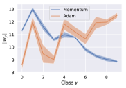
(a) CIFAR-10-LT.

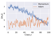
(b) CIFAR-100-LT.

Figure 1: Mean and standard deviation over $5$ runs of per-class weight norms for a ResNet-32 under momentum and Adam optimisers. We use long-tailed (“LT”) versions of CIFAR-10 and CIFAR-100, and sort classes in descending order of frequency; the first class is 100 times more likely to appear than the last class. Both optimisers yield solutions with comparable balanced error. However, the weight norms have incompatible trends: under momentum, the norms are strongly correlated with class frequency, while with Adam, the norms are anti-correlated or independent of the class frequency. Consequently, weight normalisation under Adam is ineffective for combatting class imbalance.

Loss modification. A classic means of coping with class imbalance is to balance the loss, wherein $\ell(y,f(x))$ is weighted by $\mathbb{P}(y)^{-1}$ (Xie and Manski, 1989; Morik et al., 1999): for example,

$$\ell(y,f(x))=\frac{1}{\mathbb{P}(y)}\cdot\log\Big{[}1+\sum\nolimits_{y^{\prime}\neq y}e^{f_{y^{\prime}}(x)-f_{y}(x)}\Big{]}.$$ (4)

While intuitive, balancing has minimal effect in separable settings: solutions that achieve zero training loss will necessarily remain optimal even under weighting (Byrd and Lipton, 2019). Intuitively, one would like instead to shift the separator closer to a dominant class. Li et al. (2002); Wu et al. (2008); Masnadi-Shirazi and Vasconcelos (2010); Iranmehr et al. (2019); Gottlieb et al. (2020) thus proposed to add per-class margins into the hinge loss. (Cao et al., 2019) proposed to add a per-class margin into the softmax cross-entropy:

$$\ell(y,f(x))=\log\Big{[}1+\sum\nolimits_{y^{\prime}\neq y}e^{\delta_{y}}\cdot e^{f_{y^{\prime}}(x)-f_{y}(x)}\Big{]},$$ (5)

where $\delta_{y}\propto\mathbb{P}(y)^{-1/4}$. This upweights rare “positive” labels $y$, which enforces a larger margin between a rare positive $y$ and any “negative” $y^{\prime}\neq y$. Separately, Tan et al. (2020) proposed

$$\ell(y,f(x))=\log\Big{[}1+\sum\nolimits_{y^{\prime}\neq y}e^{\delta_{y^{\prime}}}\cdot e^{f_{y^{\prime}}(x)-f_{y}(x)}\Big{]},$$ (6)

where $\delta_{y^{\prime}}\leq 0$ is an non-decreasing transform of $\mathbb{P}(y^{\prime})$. The motivation is that, in the original softmax cross-entropy without $\{\delta_{y^{\prime}}\}$, a rare label often receives a strong inhibitory gradient signal as it disproportionately appear as a negative for dominant labels. See also Liu et al. (2016, 2017); Wang et al. (2018); Khan et al. (2019) for similar weighting of negatives in the softmax.

Limitations of existing approaches. Each of the above methods are intuitive, and have shown strong empirical performance. However, a closer analysis identifies some subtle limitations.

Limitations of weight normalisation. Post-hoc weight normalisation with $\nu_{y}=\|w_{y}\|_{2}$ per Kang et al. (2020) is motivated by the observation that the weight norm $\|w_{y}\|_{2}$ tends to correlate with $\mathbb{P}(y)$. However, we now show this assumption is highly dependent on the choice of optimiser.

We consider long-tailed versions of CIFAR-10 and CIFAR-100, wherein the first class is 100 times more likely to appear than the last class. (See §6.2 for more details on these datasets.) We optimise a ResNet-32 using both SGD with momentum and Adam optimisers. Figure 1 confirms that under SGD, $\|w_{y}\|_{2}$ and the class priors $\mathbb{P}(y)$ are correlated. However, with Adam, the norms are either anti-correlated or independent of the class priors. This marked difference may be understood in light of recent study of the implicit bias of optimisers (Soudry et al., 2018); cf. Appendix F. One may hope to side-step this by simply using $\nu_{y}=\mathbb{P}(y)$; unfortunately, even this choice has limitations (see §4.2).

Limitations of loss modification. Enforcing a per-label margin per (5) and (6) is intuitive, as it allows for shifting the decision boundary away from rare classes. However, when doing so, it is important to ensure Fisher consistency (Lin, 2004) (or classification calibration (Bartlett et al., 2006)) of the resulting loss for the balanced error. That is, the minimiser of the expected loss (equally, the empirical risk in the infinite sample limit) should result in a minimal balanced error. Unfortunately, both (5) and (6) are not consistent in this sense, even for binary problems; see §5.2, §6.1 for details.

3 Logit adjustment for long-tail learning: a statistical view

The above suggests there is scope for improving performance on long-tail problems, both in terms of post-hoc correction and loss modification. We now show how a statistical perspective on the problem suggests simple procedures of each type, both of which overcome the limitations discussed above.

Recall that our goal is to minimise the balanced error (2). A natural question is: what is the best possible or Bayes-optimal scorer for this problem, i.e., $f^{*}\in\operatorname{argmin}_{f\colon\mathscr{X}\to\mathbb{R}^{L}}{\mathrm{BER}(f)}.$ Evidently, such an $f^{*}$ must depend on the (unknown) underlying distribution $\mathbb{P}(x,y)$. Indeed, we have (Menon et al., 2013), (Collell et al., 2016, Theorem 1)

$${\operatorname{argmax}\nolimits_{y\in[L]}}\,f^{*}_{y}(x)={\operatorname{argmax}\nolimits_{y\in[L]}}\,\mathbb{P}^{\mathrm{bal}}(y\mid x)={\operatorname{argmax}\nolimits_{y\in[L]}}\,\mathbb{P}(x\mid y),$$ (7)

where $\mathbb{P}^{\mathrm{bal}}$ is the balanced class-probability as per §2. In words, the Bayes-optimal prediction is the label under which the given instance $x\in\mathscr{X}$ is most likely. Consequently, for fixed class-conditionals $\mathbb{P}(x\mid y)$, varying the class priors $\mathbb{P}(y)$ arbitrarily will not affect the optimal scorers. This is intuitively desirable: the balanced error is agnostic to the level of imbalance in the label distribution.

To further probe (7), suppose the underlying class-probabilities $\mathbb{P}(y\mid x)\propto\exp(s^{*}_{y}(x))$, for (unknown) scorer $s^{*}\colon\mathscr{X}\to\mathbb{R}^{L}$. Since by definition $\mathbb{P}^{\mathrm{bal}}(y\mid x)\propto{\mathbb{P}(y\mid x)}/{\mathbb{P}(y)}$, (7) becomes

$${\operatorname{argmax}\nolimits_{y\in[L]}}\,\mathbb{P}^{\mathrm{bal}}(y\mid x)={\operatorname{argmax}\nolimits_{y\in[L]}}\,{\exp(s^{*}_{y}(x))}/{\mathbb{P}(y)}={\operatorname{argmax}\nolimits_{y\in[L]}}\,s^{*}_{y}(x)-\ln\mathbb{P}(y),$$ (8)

i.e., we translate the (unknown) distributional scores or logits based on the class priors. This simple fact immediately suggests two means of optimising for the balanced error:

1. train a model to estimate the standard $\mathbb{P}(y\mid x)$ (e.g., by minimising the standard softmax-cross entropy on the long-tailed data), and then explicitly modify its logits post-hoc as per (8)

2. train a model to estimate the balanced $\mathbb{P}^{\mathrm{bal}}(y\mid x)$, whose logits are implicitly modified as per (8)

Such logit adjustment techniques — which have been a classic approach to class-imbalance (Provost, 2000) — neatly align with the post-hoc and loss modification streams discussed in §2. However, unlike most previous techniques from these streams, logit adjustment is endowed with a clear statistical grounding: by construction, the optimal solution under such adjustment coincides with the Bayes-optimal solution (7) for the balanced error, i.e., it is Fisher consistent for minimising the balanced error. We shall demonstrate this translates into superior empirical performance (§6). Note also that logit adjustment may be easily extended to cover performance measures beyond the balanced error, e.g., with distinct costs for errors on dominant and rare classes; we leave a detailed study and contrast to existing cost-sensitive approaches (Iranmehr et al., 2019; Gottlieb et al., 2020) to future work.

We now study each of the techniques (i) and (ii) in turn.

4 Post-hoc logit adjustment

We now detail to perform post-hoc logit adjustment on a classifier trained on long-tailed data. We further show this bears similarity to recent weight normalisation schemes, but has a subtle advantage.

4.1 The post-hoc logit adjustment procedure

Given a sample $S\sim\mathbb{P}^{N}$ of long-tailed data, suppose we learn a neural network with logits $f_{y}(x)=w_{y}^{\top}\Phi(x)$. Given these, one typically predicts the label $\operatorname{argmax}_{y\in[L]}{f_{y}(x)}$. When trained with the softmax cross-entropy, one may view $p_{y}(x)\propto\exp(f_{y}(x))$ as an approximation of the underlying $\mathbb{P}(y\mid x)$, and so this equivalently predicts the label with highest estimated class-probability.

In post-hoc logit adjustment, we propose to instead predict, for suitable $\tau>0$:

$${\operatorname{argmax}\nolimits_{y\in[L]}}\,{\exp(w_{y}^{\top}\Phi(x))}/{\pi_{y}^{\tau}}={\operatorname{argmax}\nolimits_{y\in[L]}}\,f_{y}(x)-{\tau\cdot\log\pi_{y}},$$ (9)

where $\pi\in\Delta_{\mathscr{Y}}$ are estimates of the class priors $\mathbb{P}(y)$, e.g., the empirical class frequencies on the training sample $S$. Effectively, (9) adds a label-dependent offset to each of the logits. When $\tau=1$, this can be seen as applying (8) with a plugin estimate of $\mathbb{P}(y\mid x)$, i.e., ${p}_{y}(x)\propto\exp(w_{y}^{\top}\Phi(x))$. When $\tau\neq 1$, this can be seen as applying (8) to temperature scaled estimates $\bar{p}_{y}(x)\propto\exp(\tau^{-1}\cdot w_{y}^{\top}\Phi(x)).$ To unpack this, recall that (8) justifies post-hoc logit thresholding given access to the true probabilities $\mathbb{P}(y\mid x)$. In principle, the outputs of a sufficiently high-capacity neural network aim to mimic these probabilities. In practice, these estimates are often uncalibrated (Guo et al., 2017). One may thus need to first calibrate the probabilities before applying logit adjustment. Temperature scaling is one means of doing so, and is often used in the context of distillation (Hinton et al., 2015).

One may treat $\tau$ as a tuning parameter to be chosen based on some measure of holdout calibration, e.g., the expected calibration error (Murphy and Winkler, 1987; Guo et al., 2017), probabilistic sharpness (Gneiting et al., 2007; Kuleshov et al., 2018), or a proper scoring rule such as the log-loss or squared error (Gneiting and Raftery, 2007). One may alternately fix $\tau=1$ and aim to learn inherently calibrated probabilities, e.g., via label smoothing (Szegedy et al., 2016; Müller et al., 2019).

4.2 Comparison to existing post-hoc techniques

Post-hoc logit adjustment with $\tau=1$ is not a new idea in the class imbalance literature. Indeed, this is a standard technique when creating stratified samples (King and Zeng, 2001), and when training binary classifiers  (Fawcett and Provost, 1996; Provost, 2000; Maloof, 2003). In multiclass settings, this has been explored in Zhou and Liu (2006); Collell et al. (2016). However, $\tau\neq 1$ is important in practical usage of neural networks, owing to their lack of calibration. Further, we now explicate that post-hoc logit adjustment has an important advantage over recent post-hoc weight normalisation techniques.

Recall that weight normalisation involves learning a scorer $f_{y}(x)=w_{y}^{\top}\Phi(x)$, and then post-hoc normalising the weights via ${w_{y}}/{\nu_{y}^{\tau}}$ for $\tau>0$. We demonstrated in §2 that using $\nu_{y}=\|w_{y}\|_{2}$ may be ineffective when using adaptive optimisers. However, even with $\nu_{y}=\pi_{y}$, there is a subtle contrast to post-hoc logit adjustment: while the former performs a multiplicative update to the logits, the latter performs an additive update. The two techniques may thus yield different orderings over labels, since

$$\frac{w_{1}^{\mathrm{T}}\Phi(x)}{\pi_{1}}<\frac{w_{2}^{\mathrm{T}}\Phi(x)}{\pi_{2}}<\cdots<\frac{w_{L}^{\mathrm{T}}\Phi(x)}{\pi_{L}}\begin{subarray}{c}\centernot\implies\\ \centernot\impliedby\end{subarray}\frac{e^{w_{1}^{\mathrm{T}}\Phi(x)}}{\pi_{1}}<\frac{e^{w_{2}^{\mathrm{T}}\Phi(x)}}{\pi_{2}}<\cdots<\frac{e^{w_{L}^{\mathrm{T}}\Phi(x)}}{\pi_{L}}.$$

Weight normalisation is thus not consistent for minimising the balanced error, unlike logit adjustment. Indeed, if a rare label $y$ has negative score $w_{y}^{\top}\Phi(x)<0$, and there is another label with positive score, then it is impossible for the weight normalisation to give $y$ the highest score. By contrast, under logit adjustment, $w_{y}^{\mathrm{T}}\Phi(x)-\ln\pi_{y}$ will be lower for dominant classes, regardless of the original sign.

5 The logit adjusted softmax cross-entropy

We now show how to directly bake logit adjustment into the softmax cross-entropy. We show that this approach has an intuitive relation to existing loss modification techniques.

5.1 The logit adjusted loss

From §3, the second approach to optimising for the balanced error is to directly model $\mathbb{P}_{\mathrm{bal}}(y\mid x)\propto{\mathbb{P}(y\mid x)}/{\mathbb{P}(y)}$. To do so, consider the following logit adjusted softmax cross-entropy loss for $\tau>0$:

Given a scorer that minimises the above, we now predict ${\operatorname{argmax}}_{y\in[L]}f_{y}(x)$ as usual.

Compared to the standard softmax cross-entropy (1), the above applies a label-dependent offset to each logit. Compared to (9), we directly enforce the class prior offset while learning the logits, rather than doing this post-hoc. The two approaches have a deeper connection: observe that (10) is equivalent to using a scorer of the form $g_{y}(x)=f_{y}(x)+\tau\cdot\log\pi_{y}$. We thus have ${\operatorname{argmax}}_{y\in[L]}f_{y}(x)={\operatorname{argmax}}_{y\in[L]}g_{y}(x)-\tau\cdot\log\pi_{y}$. Consequently, one can equivalently view learning with this loss as learning a standard scorer $g(x)$, and post-hoc adjusting its logits to make a prediction. For convex objectives, we thus do not expect any difference between the solutions of the two approaches. For non-convex objectives, as encountered in neural networks, the bias endowed by adding $\tau\cdot\log\pi_{y}$ to the logits is however likely to result in a different local minima.

For more insight into the loss, consider the following pairwise margin loss

$$\ell(y,f(x)) =\alpha_{y}\cdot\log\Big{[}1+\sum\nolimits_{y^{\prime}\neq y}e^{\Delta_{yy^{\prime}}}\cdot e^{(f_{y^{\prime}}(x)-f_{y}(x))}\Big{]},$$ (11)

for label weights $\alpha_{y}>0$, and pairwise label margins $\Delta_{yy^{\prime}}$ representing the desired gap between scores for $y$ and $y^{\prime}$. For $\tau=1$, our logit adjusted loss (10) corresponds to (11) with $\alpha_{y}=1$ and $\Delta_{yy^{\prime}}=\log\left(\frac{\pi_{y^{\prime}}}{\pi_{y}}\right)$. This demands a larger margin between rare positive ($\pi_{y}\sim 0$) and dominant negative ($\pi_{y^{\prime}}\sim 1$) labels, so that scores for dominant classes do not overwhelm those for rare ones.

5.2 Comparison to existing loss modification techniques

A cursory inspection of (5), (6) reveals a striking similarity to our logit adjusted softmax cross-entropy (10). The balanced loss (4) also bears similarity, except that the weighting is performed outside the logarithm. Each of these losses are special cases of the pairwise margin loss (11) enforcing uniform margins that only consider the positive or negative label, unlike our approach.

For example, $\alpha_{y}=\frac{1}{\pi_{y}}$ and $\Delta_{yy^{\prime}}=0$ yields the balanced loss (4). This does not explicitly enforce a margin between the labels, which is undesirable for separable problems (Byrd and Lipton, 2019). When $\alpha_{y}=1$, the choice $\Delta_{yy^{\prime}}=\pi_{y}^{-1/4}$ yields (5). Finally, $\Delta_{yy^{\prime}}=\log F(\pi_{y^{\prime}})$ yields (6), where $F\colon[0,1]\to(0,1]$ is some non-decreasing function, e.g., $F(z)=z^{\tau}$ for $\tau>0$. These losses thus either consider the frequency of the positive $y$ or negative $y^{\prime}$, but not both simultaneously.

The above choices of $\alpha$ and $\Delta$ are all intuitively plausible. However, §3 indicates that our loss in (10) has a firm statistical grounding: it ensures Fisher consistency for the balanced error.

Theorem 1.

For any $\delta\in\mathbb{R}_{+}^{L}$, the pairwise loss in (11) is Fisher consistent with weights and margins

$$\alpha_{y} ={\delta_{y}}/{\pi_{y}}\qquad\Delta_{yy^{\prime}}=\log\big{(}{\delta_{y^{\prime}}}/{\delta_{y}}\big{)}.$$

Observe that when $\delta_{y}=\pi_{y}$, we immediately deduce that the logit-adjusted loss of (10) is consistent. Similarly, $\delta_{y}=1$ recovers the classic result that the balanced loss is consistent. While the above is only a sufficient condition, it turns out that in the binary case, one may neatly encapsulate a necessary and sufficient condition for consistency that rules out other choices; see Appendix B.1. This suggests that existing proposals may thus underperform with respect to the balanced error in certain settings, as verified empirically in §6.1.

5.3 Discussion and extensions

One may be tempted to combine the logit adjusted loss in (10) with the post-hoc adjustment of (9). However, following §3, such an approach would not be statistically coherent. Indeed, minimising a logit adjusted loss encourages the model to estimate the balanced class-probabilities $\mathbb{P}^{\mathrm{bal}}(y\mid x)$. Applying post-hoc adjustment will distort these probabilities, and is thus expected to be harmful.

More broadly, however, there is value in combining logit adjustment with other techniques. For example, Theorem 1 implies that it is sensible to combine logit adjustment with loss weighting; e.g., one may pick $\Delta_{yy^{\prime}}={\tau}\cdot\log\left({{\pi_{y^{\prime}}}/{\pi_{y}}}\right)$, and $\alpha_{y}=\pi_{y}^{\tau-1}$. This is similar to Cao et al. (2019), who found benefits in combining weighting with their loss. One may also generalise the formulation in Theorem 1, and employ $\Delta_{yy^{\prime}}=\tau_{1}\cdot\log\pi_{y}-\tau_{2}\cdot\log\pi_{y^{\prime}}$, where $\tau_{1},\tau_{2}$ are constants. This interpolates between the logit adjusted loss ($\tau_{1}=\tau_{2}$) and a version of the equalised margin loss ($\tau_{1}=0$).

Cao et al. (2019, Theorem 2) provides a rigorous generalisation bound for the adaptive margin loss under the assumption of separable training data with binary labels. The inconsistency of the loss with respect to the balanced error concerns the more general scenario of non-separable multiclass data data, which may occur, e.g., owing to label noise or limitation in model capacity. We shall subsequently demonstrate that encouraging consistency can lead to gains in practical settings. We shall further see that combining the $\Delta$ implicit in this loss with our proposed $\Delta$ can lead to further gains, indicating a potentially complementary nature of the losses.

Interestingly, for $\tau=-1$, a similar loss to (10) has been considered in the context of negative sampling for scalability (Yi et al., 2019): here, one samples a small subset of negatives based on the class priors $\pi$, and applies logit correction to obtain an unbiased estimate of the unsampled loss function based on all the negatives (Bengio and Senecal, 2008). Losses of the general form (11) have also been explored for structured prediction (Zhang, 2004; Pletscher et al., 2010; Hazan and Urtasun, 2010).

6 Experimental results

We now present experiments confirming our main claims: (i) on simple binary problems, existing weight normalisation and loss modification techniques may not converge to the optimal solution (§6.1); (ii) on real-world datasets, our post-hoc logit adjustment outperforms weight normalisation, and one can obtain further gains via our logit adjusted softmax cross-entropy (§6.2).

6.1 Results on synthetic dataset

We consider a binary classification task, wherein samples from class $y\in\{\pm 1\}$ are drawn from a 2D Gaussian with isotropic covariance and means $\mu_{y}=y\cdot(+1,+1)$. We introduce class imbalance by setting $\mathbb{P}(y=+1)=5\%$. The Bayes-optimal classifier for the balanced error is (see Appendix G)

$$f^{*}(x)=+1\iff\mathbb{P}(x\mid y=+1)>\mathbb{P}(x\mid y=-1)\iff(\mu_{1}-\mu_{-1})^{\top}x>0,$$ (12)

i.e., it is a linear separator passing through the origin. We compare this separator against those found by several margin losses based on (11): standard ERM ($\Delta_{yy^{\prime}}=0$), the adaptive loss (Cao et al., 2019) ($\Delta_{yy^{\prime}}=\pi_{y}^{-1/4}$), an instantiation of the equalised loss (Tan et al., 2020) ($\Delta_{yy^{\prime}}=\log\pi_{y^{\prime}}$), and our logit adjusted loss ($\Delta_{yy^{\prime}}=\log\frac{\pi_{y^{\prime}}}{\pi_{y}}$). For each loss, we train an affine classifier on a sample of $10,000$ instances, and evaluate the balanced error on a test set of $10,000$ samples over $100$ independent trials.

Figure 2 confirms that the logit adjusted margin loss attains a balanced error close to that of the Bayes-optimal, which is visually reflected by its learned separator closely matching that in (12). This is in line with our claim of the logit adjusted margin loss being consistent for the balanced error, unlike other approaches. Figure 2 also compares post-hoc weight normalisation and logit adjustment for varying scaling parameter $\tau$ (c.f. (3), (9)). Logit adjustment is seen to approach the performance of the Bayes predictor; any weight normalisation is however seen to hamper performance. This verifies the consistency of logit adjustment, and inconsistency of weight normalisation (§4.2).

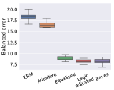
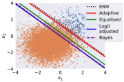
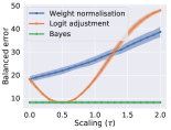
Figure 2: Results on synthetic binary classification problem. Our logit adjusted loss tracks the Bayes-optimal solution and separator (left & middle panel). Post-hoc logit adjustment matches the Bayes performance with suitable scaling (right panel); however, any weight normalisation fails.

6.2 Results on real-world datasets

We present results on the CIFAR-10, CIFAR-100, ImageNet and iNaturalist 2018 datasets. Following prior work, we create “long-tailed versions” of the CIFAR datasets by suitably downsampling examples per label following the Exp profile of Cui et al. (2019); Cao et al. (2019) with imbalance ratio $\rho={\max_{y}\mathbb{P}(y)}/{\min_{y}\mathbb{P}(y)}=100$. Similarly, we use the long-tailed version of ImageNet produced by Liu et al. (2019). We employ a ResNet-32 for CIFAR, and a ResNet-50 for ImageNet and iNaturalist. All models are trained using SGD with momentum; see Appendix D for more details. See also Appendix E.1 for results on CIFAR under the Step profile considered in the literature.

Method	CIFAR-10-LT	CIFAR-100-LT	ImageNet-LT	iNaturalist
ERM	27.16	61.64	53.11	38.66
Weight normalisation ($\tau=1$) (Kang et al., 2020)	24.02	58.89	52.00	48.05
Weight normalisation ($\tau=\tau^{*}$) (Kang et al., 2020)	21.50	58.76	49.37	34.10⋆
Adaptive (Cao et al., 2019)	26.65†	60.40†	52.15	35.42†
Equalised (Tan et al., 2020)	26.02	57.26	54.02	38.37
Logit adjustment post-hoc ($\tau=1$)	22.60	58.24	49.66	33.98
Logit adjustment post-hoc ($\tau=\tau^{*}$)	19.08	57.90	49.56	33.80
Logit adjustment loss ($\tau=1$)	22.33	56.11	48.89	33.64

Table 3: Test set balanced error (averaged over $5$ trials) on real-world datasets. We use a ResNet-32 for the CIFAR datasets, and ResNet-50 for the ImageNet and iNaturalist datasets. Here, ^†, ^⋆ are numbers for “LDAM + SGD” from Cao et al. (2019, Table 2, 3) and “$\tau$-normalised” from Kang et al. (2020, Table 3, 7). Here, $\tau=\tau^{*}$ refers to using the best possible value of tuning parameter $\tau$. See Figure 3 for plots as a function of $\tau$, and the “Discussion” subsection for further extensions.

Baselines. We consider: (i) empirical risk minimisation (ERM) on the long-tailed data, (ii) post-hoc weight normalisation (Kang et al., 2020) per (3) (using $\nu_{y}=\|w_{y}\|_{2}$ and $\tau=1$) applied to ERM, (iii) the adaptive margin loss (Cao et al., 2019) per (5), and (iv) the equalised loss (Tan et al., 2020) per (6), with $\delta_{y^{\prime}}=F(\pi_{y^{\prime}})$ for the threshold-based $F$ of Tan et al. (2020). Cao et al. (2019) demonstrated superior performance of their adaptive margin loss against several other baselines, such as the balanced loss of (4), and that of Cui et al. (2019). Where possible, we report numbers for the baselines (which use the same setup as above) from the respective papers. See also our concluding discussion about extensions to such methods that improve performance.

We compare the above methods against our proposed post-hoc logit adjustment (9), and logit adjusted loss (10). For post-hoc logit adjustment, we fix the scalar $\tau=1$; we analyse the effect of tuning this in Figure 3. We do not perform any further tuning of our logit adjustment techniques.

Results and analysis. Table 3 summarises our results, which demonstrate our proposed logit adjustment techniques consistently outperform existing methods. Indeed, while weight normalisation offers gains over ERM, these are improved significantly by post-hoc logit adjustment (e.g., 8% relative reduction on CIFAR-10). Similarly loss correction techniques are generally outperformed by our logit adjusted softmax cross-entropy (e.g., 6% relative reduction on iNaturalist).

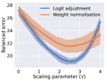
(a) CIFAR-10.

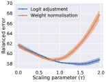
(b) CIFAR-100.

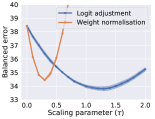
(c) iNaturalist.

Figure 3: Comparison of balanced error for post-hoc correction techniques when varying scaling parameter $\tau$ (c.f. (3), (9)). Post-hoc logit adjustment consistently outperforms weight normalisation.

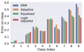
(a) CIFAR-10.

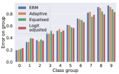
(b) CIFAR-100.

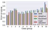
(c) iNaturalist.

Figure 4: Per-class error rates of loss modification techniques. For (b) and (c), we aggregate the classes into 10 groups. ERM displays a strong bias towards dominant classes (lower indices). Our proposed logit adjusted softmax loss achieves significant gains on rare classes (higher indices).

Figure 3 studies the effect of tuning the scaling parameter $\tau>0$ afforded by post-hoc weight normalisation (using $\nu_{y}=\|w_{y}\|_{2}$) and post-hoc logit adjustment. Even without any scaling, post-hoc logit adjustment generally offers superior performance to the best result from weight normalisation (cf. Table 3); with scaling, this is further improved. See Appendix 11 for a plot on ImageNet-LT.

Figure 4 breaks down the per-class accuracies on CIFAR-10, CIFAR-100, and iNaturalist. On the latter two datasets, for ease of visualisation, we aggregate the classes into ten groups based on their frequency-sorted order (so that, e.g., group $0$ comprises the top $\frac{L}{10}$ most frequent classes). As expected, dominant classes generally see a lower error rate with all methods. However, the logit adjusted loss is seen to systematically improve performance over ERM, particularly on rare classes.

While our logit adjustment techniques perform similarly, there is a slight advantage to the loss function version. Nonetheless, the strong performance of post-hoc logit adjustment corroborates the ability to decouple representation and classifier learning in long-tail settings (Zhang et al., 2019).

Discussion and extensions Table 3 shows the advantage of logit adjustment over recent post-hoc and loss modification proposals, under standard setups from the literature. We believe further improvements are possible by fusing complementary ideas, and remark on four such options.

First, one may use a more complex base architecture; our choices are standard in the literature, but, e.g., Kang et al. (2020) found gains on ImageNet-LT by employing a ResNet-152, with further gains from training it for $200$ as opposed to the customary $90$ epochs. Table 4 confirms that logit adjustment similarly benefits from this choice. For example, on iNaturalist, we obtain an improved balanced error of ${31.15}\%$ for the logit adjusted loss. When training for more ($200$) epochs per the suggestion of Kang et al. (2020), this further improves to ${30.12}\%$.

Second, one may combine together the $\Delta$’s for various special cases of the pairwise margin loss. Indeed, we find that combining our relative margin with the adaptive margin of Cao et al. (2019) — i.e., using the pairwise margin loss with $\Delta_{yy^{\prime}}=\log\frac{\pi_{y^{\prime}}}{\pi_{y}}+\frac{1}{\pi_{y}^{1/4}}$ — results in a top-$1$ accuracy of ${31.56}\%$ on iNaturalist. When using a ResNet-152, this further improves to ${29.22}\%$ when trained for 90 epochs, and $\mathbf{28.02}\%$ when trained for 200 epochs. While such a combination is nominally heuristic, we believe there is scope to formally study such schemes, e.g., in terms of induced generalisation performance.

	ImageNet-LT		iNaturalist
Method	ResNet-50	ResNet-152	ResNet-50	ResNet-152	ResNet-152
			90 epochs	90 epochs	200 epochs
ERM	53.11	53.30	38.66	35.88	34.38
Weight normalisation ($\tau=1$) (Kang et al., 2020)	52.00	51.49	48.05	45.17	45.33
Weight normalisation ($\tau=\tau^{*}$) (Kang et al., 2020)	49.37	48.97	34.10	31.85	30.34
Adaptive (Cao et al., 2019)	52.15	53.34	35.42	31.18	29.46
Equalised (Tan et al., 2020)	54.02	51.38	38.37	35.86	34.53
Logit adjustment post-hoc ($\tau=1$)	49.66	49.25	33.98	31.46	30.15
Logit adjustment post-hoc ($\tau=\tau^{*}$)	49.56	49.15	33.80	31.08	29.74
Logit adjustment loss ($\tau=1$)	48.89	47.86	33.64	31.15	30.12
Logit adjustment plus adaptive loss ($\tau=1$)	51.25	50.46	31.56	29.22	28.02

Table 4: Test set balanced error (averaged over $5$ trials) on real-world datasets with more complex base architectures. Employing a ResNet-152 is seen to systematically improve all methods’ performance, with logit adjustment remaining superior to existing approaches. The final row reports the results of combining logit adjustment with the adaptive margin loss of Cao et al. (2019), which yields further gains on iNaturalist.

Third, Cao et al. (2019) observed that their loss benefits from a deferred reweighting scheme (DRW), wherein the model begins training as normal, and then applies class-weighting after a fixed number of epochs. On CIFAR-10-LT and CIFAR-100-LT, this achieves $22.97\%$ and $57.96\%$ error respectively; both are outperformed by our vanilla logit adjusted loss. On iNaturalist with a ResNet-50, this achieves an error of $32.0\%$, outperforming our $33.6\%$. (Note that our simple combination of the relative and adaptive margins outperforms these reported numbers of DRW.) However, given the strong improvement of our loss over that in Cao et al. (2019) when both methods use SGD, we expect that employing DRW (which applies to any loss) may be similarly beneficial for our method.

Fourth, per §2, one may perform data augmentation; e.g., see Tan et al. (2020, Section 6). While further exploring such variants are of empirical interest, we hope to have illustrated the conceptual and empirical value of logit adjustment, and leave this for future work.

Supplementary material for “Long tail learning via logit adjustment”

Appendix A Proofs of results in body

Proof of Theorem 1.

Denote $\eta_{y}(x)=\mathbb{P}(y\mid x)$. Suppose we employ a margin $\Delta_{yy^{\prime}}=\log\frac{\delta_{y^{\prime}}}{\delta_{y}}$. Then, the loss is

$${\ell}(y,f(x))=-\log\frac{\delta_{y}\cdot e^{f_{y}(x)}}{\sum_{y^{\prime}\in[L]}{\delta_{y^{\prime}}}\cdot e^{f_{y^{\prime}}(x)}}=-\log\frac{e^{f_{y}(x)+\log\delta_{y}}}{\sum_{y^{\prime}\in[L]}e^{f_{y^{\prime}}(x)+\log\delta_{y^{\prime}}}}.$$

Consequently, under constant weights $\alpha_{y}=1$, the Bayes-optimal score will satisfy $f^{*}_{y}(x)+\log\delta_{y}=\log\eta_{y}(x)$, or $f^{*}_{y}(x)=\log\frac{\eta_{y}(x)}{\delta_{y}}$.

Now suppose we use generic weights $\alpha\in\mathbb{R}_{+}^{L}$. The risk under this loss is

$${\mathbb{E}}_{{x},{y}}\left[\ell_{\alpha}({y},f({x}))\right] =\sum_{y\in[L]}\pi_{y}\cdot{\mathbb{E}}_{{x}\mid{y}=y}\left[\ell_{\alpha}(y,f(x))\right]$$

$$=\sum_{y\in[L]}\pi_{y}\cdot{\mathbb{E}}_{{x}\mid{y}=y}\left[\ell_{\alpha}(y,f(x))\right]$$

$$=\sum_{y\in[L]}\pi_{y}\cdot\alpha_{y}\cdot{\mathbb{E}}_{{x}\mid{y}=y}\left[\ell(y,f(x))\right]$$

$$\propto\sum_{y\in[L]}\bar{\pi}_{y}\cdot{\mathbb{E}}_{{x}\mid{y}=y}\left[\ell(y,f(x))\right],$$

where $\bar{\pi}_{y}\propto{\pi_{y}\cdot\alpha_{y}}$. Consequently, learning with the weighted loss is equivalent to learning with the original loss, on a distribution with modified base-rates $\bar{\pi}$. Under such a distribution, we have class-conditional distribution

$$\bar{\eta}_{y}(x)=\bar{\mathbb{P}}(y\mid x)=\frac{\mathbb{P}(x\mid y)\cdot\bar{\pi}_{y}}{\bar{\mathbb{P}}(x)}=\eta_{y}(x)\cdot\frac{\bar{\pi}_{y}}{{\pi}_{y}}\cdot\frac{\mathbb{P}(x)}{\bar{\mathbb{P}}(x)}\propto\eta_{y}(x)\cdot\alpha_{y}.$$

Consequently, suppose $\alpha_{y}=\frac{\delta_{y}}{\pi_{y}}$. Then, $f^{*}_{y}(x)=\log\frac{\bar{\eta}_{y}(x)}{\delta_{y}}=\log\frac{\eta_{y}(x)}{\pi_{y}}+C(x)$, where $C(x)$ does not depend on $y$. Consequently, ${\operatorname{argmax}\nolimits_{y\in[L]}}\,f^{*}_{y}(x)={\operatorname{argmax}\nolimits_{y\in[L]}}\,\frac{\eta_{y}(x)}{\pi_{y}}$, which is the Bayes-optimal prediction for the balanced error.

In sum, a consistent family can be obtained by choosing any set of constants $\delta_{y}>0$ and setting

$$\alpha_{y} =\frac{\delta_{y}}{\pi_{y}}$$

$$\Delta_{yy^{\prime}} =\log\frac{\delta_{y^{\prime}}}{\delta_{y}}.$$

∎

Appendix B On the consistency of binary margin-based losses

It is instructive to study the pairwise margin loss (11) in the binary case. Endowing the loss with a temperature parameter $\gamma>0$, we get

$$\ell(+1,f) =\frac{\omega_{+1}}{\gamma}\cdot\log(1+e^{\gamma\cdot\delta_{+1}}\cdot e^{-\gamma\cdot f})$$ (13)

$$\ell(-1,f) =\frac{\omega_{-1}}{\gamma}\cdot\log(1+e^{\gamma\cdot\delta_{-1}}\cdot e^{\gamma\cdot f})$$

for constants $\omega_{\pm 1},\gamma>0$ and $\delta_{\pm 1}\in\mathbb{R}$. Here, we have used $\delta_{+1}=\Delta_{+1,-1}$ and $\delta_{-1}=\Delta_{-1,+1}$ for simplicity. The choice $\omega_{\pm 1}=1,\delta_{\pm 1}=0$ recovers the temperature scaled binary logistic loss. Evidently, as $\gamma\to+\infty$, these converge to weighted hinge losses with variable margins, i.e.,

$$\ell(+1,f) ={\omega_{+1}}\cdot[\delta_{+1}-f]_{+}$$

$$\ell(-1,f) ={\omega_{-1}}\cdot[\delta_{-1}+f]_{+}.$$

We study two properties of this family losses. First, under what conditions are the losses Fisher consistent for the balanced error? We shall show that in fact there is a simple condition characterising this. Second, do the losses preserve properness of the original binary logistic loss? We shall show that this is always the case, but that the losses involve fundamentally different approximations.

B.1 Consistency of the binary pairwise margin loss

Given a loss $\ell$, its Bayes optimal solution is $f^{*}\in\operatorname{argmin}_{f\colon\mathscr{X}\to\mathbb{R}}{\mathbb{E}}\left[\ell({y},f({x}))\right]$. For consistency with respect to the balanced error in the binary case, we require this optimal solution $f^{*}$ to satisfy $f^{*}(x)>0\iff{\eta(x)>\pi}$, where $\eta(x)\stackrel{{\scriptstyle.}}{{=}}\mathbb{P}(y=1\mid x)$ and $\pi\stackrel{{\scriptstyle.}}{{=}}\mathbb{P}(y=1)$ [Menon et al., 2013]. This is equivalent to a simple condition on the weights $\omega$ and margins $\delta$ of the pairwise margin loss.

Lemma 2.

The losses in (13) are consistent for the balanced error iff

$$\frac{\omega_{+1}}{\omega_{-1}}\cdot\frac{\sigma(\gamma\cdot\delta_{+1})}{\sigma(\gamma\cdot\delta_{-1})}=\frac{1-\pi}{\pi},$$

where $\sigma(z)=(1+\exp(z))^{-1}$.

Proof of Lemma 2.

Denote $\eta(x)\stackrel{{\scriptstyle.}}{{=}}\mathbb{P}(y=+1\mid x)$, and $\pi\stackrel{{\scriptstyle.}}{{=}}\mathbb{P}(y=+1)$. From Lemma 3 below, the pairwise margin loss is proper composite with invertible link function $\Psi\colon[0,1]\to\mathbb{R}\cup\{\pm\infty\}$. Consequently, since by definition the Bayes-optimal score for a proper composite loss is $f^{*}(x)=\Psi(\eta(x))$ [Reid and Williamson, 2010], to have consistency for the balanced error, from (14), (15), we require

$$\Psi^{-1}(0)=\pi \iff\frac{1}{1-\frac{\ell^{\prime}(+1,0)}{\ell^{\prime}(-1,0)}}=\pi$$

$$\iff{1-\frac{\ell^{\prime}(+1,0)}{\ell^{\prime}(-1,0)}}=\frac{1}{\pi}$$

$$\iff{-\frac{\ell^{\prime}(+1,0)}{\ell^{\prime}(-1,0)}}=\frac{1-\pi}{\pi}$$

$$\iff\frac{\omega_{+1}}{\omega_{-1}}\cdot\frac{\sigma(\gamma\cdot\delta_{+1})}{\sigma(\gamma\cdot\delta_{-1})}=\frac{1-\pi}{\pi}.$$

∎

From the above, some admissible parameter choices include:

• $\omega_{+1}=\frac{1}{\pi}$, $\omega_{-1}=\frac{1}{1-\pi}$, $\delta_{\pm 1}=1$; i.e., the standard weighted loss with a constant margin

• $\omega_{\pm 1}=1$, $\delta_{+1}=\frac{1}{\gamma}\cdot\log\frac{1-\pi}{\pi}$, $\delta_{-1}=\frac{1}{\gamma}\cdot\log\frac{\pi}{1-\pi}$; i.e., the unweighted loss with a margin biased towards the rare class, as per our logit adjustment procedure

The second example above is unusual in that it requires scaling the margin with the temperature; consequently, the margin disappears as $\gamma\to+\infty$. Other combinations are of course possible, but note that one cannot arbitrarily choose parameters and hope for consistency in general. Indeed, some inadmissible choices are naïve applications of the margin modification or weighting, e.g.,

• $\omega_{+1}=\frac{1}{\pi}$, $\omega_{-1}=\frac{1}{1-\pi}$, $\delta_{+1}=\frac{1}{\gamma}\cdot\log\frac{1-\pi}{\pi}$, $\delta_{-1}=\frac{1}{\gamma}\cdot\log\frac{\pi}{1-\pi}$; i.e., combining both weighting and margin modification

• $\omega_{\pm 1}=1$, $\delta_{+1}=\frac{1}{\gamma}\cdot(1-\pi)$, $\delta_{-1}=\frac{1}{\gamma}\cdot{\pi}$; i.e., specific margin modification

Note further that the choices of Cao et al. [2019], Tan et al. [2020] do not meet the requirements of Lemma 2.

We make two final remarks. First, the above only considers consistency of the result of loss minimisation. For any choice of weights and margins, we may apply suitable post-hoc correction to the predictions to account for any bias in the optimal scores. Second, as $\gamma\to+\infty$, any constant margins $\delta_{\pm 1}>0$ will have no effect on the consistency condition, since $\sigma(\gamma\cdot\delta_{\pm 1})\to 1$. The condition will be wholly determined by the weights $\omega_{\pm 1}$. For example, we may choose $\omega_{+1}=\frac{1}{\pi}$, $\omega_{-1}=\frac{1}{1-\pi}$, $\delta_{+1}=1$, and $\delta_{-1}=\frac{\pi}{1-\pi}$; the resulting loss will not be consistent for finite $\gamma$, but will become so in the limit $\gamma\to+\infty$. For more discussion on this particular loss, see Appendix C.

B.2 Properness of the pairwise margin loss

In the above, we appealed to the pairwise margin loss being proper composite, in the sense of Reid and Williamson [2010]. Intuitively, this specifies that the loss has Bayes-optimal score of the form $f^{*}(x)=\Psi(\eta(x))$, where $\Psi$ is some invertible function, and $\eta(x)=\mathbb{P}(y=1\mid x)$. We have the following general result about properness of any member of the pairwise margin family.

Lemma 3.

The losses in (13) are proper composite, with link function

$$\Psi(p) =\frac{1}{\gamma}\cdot\log\left[\left(\frac{a\cdot b}{q}-c\right)\pm\sqrt{\left(\frac{a\cdot b}{q}-c\right)^{2}+4\cdot\frac{a}{q}}\right]-\log 2,$$

where $a=\frac{\omega_{+1}}{\omega_{-1}}\cdot\frac{e^{\gamma\cdot\delta_{+1}}}{e^{\gamma\cdot\delta_{-1}}}$, $b=e^{\gamma\cdot\delta_{-1}}$, $c=e^{\gamma\cdot\delta_{+1}}$, and $q=\frac{1-p}{p}$.

Proof of Lemma 3.

The above family of losses is proper composite iff the function

$$\Psi^{-1}(f)=\frac{1}{1-\frac{\ell^{\prime}(+1,f)}{\ell^{\prime}(-1,f)}}$$ (14)

is invertible [Reid and Williamson, 2010, Corollary 12]. We have

$$\ell^{\prime}(+1,f) =-{\omega_{+1}}\cdot\frac{e^{\gamma\cdot\delta_{+1}}\cdot e^{-\gamma\cdot f}}{1+e^{\gamma\cdot\delta_{+1}}\cdot e^{-\gamma\cdot f}}$$ (15)

$$\ell^{\prime}(-1,f) =+{\omega_{-1}}\cdot\frac{e^{\gamma\cdot\delta_{-1}}\cdot e^{\gamma\cdot f}}{1+e^{\gamma\cdot\delta_{-1}}\cdot e^{\gamma\cdot f}}.$$

The invertibility of $\Psi^{-1}$ is immediate. To compute the link function $\Psi$, note that

$$p=\frac{1}{1-\frac{\ell^{\prime}(+1,f)}{\ell^{\prime}(-1,f)}} \iff\frac{1}{p}=1-\frac{\ell^{\prime}(+1,f)}{\ell^{\prime}(-1,f)}$$

$$\iff-\frac{\ell^{\prime}(+1,f)}{\ell^{\prime}(-1,f)}=\frac{1-p}{p}$$

$$\iff\frac{\omega_{+1}}{\omega_{-1}}\cdot\frac{e^{\gamma\cdot\delta_{+1}}\cdot e^{-\gamma\cdot f}}{1+e^{\gamma\cdot\delta_{+1}}\cdot e^{-\gamma\cdot f}}\cdot\frac{1+e^{\gamma\cdot\delta_{-1}}\cdot e^{\gamma\cdot f}}{e^{\gamma\cdot\delta_{-1}}\cdot e^{\gamma\cdot f}}=\frac{1-p}{p}$$

$$\iff\frac{\omega_{+1}}{\omega_{-1}}\cdot\frac{e^{\gamma\cdot\delta_{+1}}}{e^{\gamma\cdot\delta_{-1}}}\cdot\frac{1}{e^{\gamma\cdot f}+e^{\gamma\cdot\delta_{+1}}}\cdot\frac{1+e^{\gamma\cdot\delta_{-1}}\cdot e^{\gamma\cdot f}}{e^{\gamma\cdot f}}=\frac{1-p}{p}$$

$$\iff a\cdot\frac{1+b\cdot g}{g^{2}+c\cdot g}=q,$$

where $a=\frac{\omega_{+1}}{\omega_{-1}}\cdot\frac{e^{\gamma\cdot\delta_{+1}}}{e^{\gamma\cdot\delta_{-1}}}$, $b=e^{\gamma\cdot\delta_{-1}}$, $c=e^{\gamma\cdot\delta_{+1}}$, $g=e^{\gamma\cdot f}$, and $q=\frac{1-p}{p}$. Thus,

$$a\cdot\frac{1+b\cdot g}{g^{2}+c\cdot g}=q \iff\frac{g^{2}+c\cdot g}{1+b\cdot g}=\frac{a}{q}$$

$$\iff g^{2}+\left(c-\frac{a\cdot b}{q}\right)\cdot g-\frac{a}{q}=0$$

$$\iff g=\frac{\left(\frac{a\cdot b}{q}-c\right)\pm\sqrt{\left(\frac{a\cdot b}{q}-c\right)^{2}+4\cdot\frac{a}{q}}}{2}.$$

∎

As a sanity check, suppose $a=b=c=\gamma=1$. This corresponds to the standard logistic loss. Then,

$$\Psi(p)=\log\frac{\left(\frac{1}{q}-1\right)\pm\sqrt{\left(\frac{1}{q}-1\right)^{2}+4\cdot\frac{1}{q}}}{2}=\log\frac{p}{1-p},$$

which is the standard logit function.

Figure 5 and 6 compares the link functions for a few different settings:

• the balanced loss, where $\omega_{+1}=\frac{1}{\pi}$, $\omega_{-1}=\frac{1}{1-\pi}$, and $\delta_{\pm 1}=1$

• an unequal margin loss, where $\omega_{\pm 1}=1$, $\delta_{+1}=\frac{1}{\gamma}\cdot\log\frac{1-\pi}{\pi}$, and $\delta_{-1}=\frac{1}{\gamma}\cdot\log\frac{\pi}{1-\pi}$

• a balanced + margin loss, where $\omega_{+1}=\frac{1}{\pi}$, $\omega_{-1}=\frac{1}{1-\pi}$, $\delta_{+1}=1$, and $\delta_{-1}=\frac{\pi}{1-\pi}$.

The property $\Psi^{-1}(0)=\pi$ for $\pi=\mathbb{P}(y=1)$ holds for the first two choices with any $\gamma>0$, and the third choice as $\gamma\to+\infty$. This indicates the Fisher consistency of these losses for the balanced error. However, the precise way this is achieved is strikingly different in each case. In particular, each loss implicitly involves a fundamentally different link function.

To better understand the effect of parameter choices, Figure 7 illustrates the conditional Bayes risk curves, i.e.,

$$\underline{L}(p)=p\cdot\ell(+1,\Psi(p))+(1-p)\cdot\ell(+1,\Psi(p)).$$

We remark here that for the balanced error, this function takes the form $\underline{L}(p)=p\cdot\llbracket p<\pi\rrbracket+(1-p)\cdot\llbracket p>\pi\rrbracket$, i.e., it is a “tent shaped” concave function with a maximum at $p=\pi$.

For ease of comparison, we normalise this curves to have a maximum of $1$. Figure 7 shows that simply applying unequal margins does not affect the underlying conditional Bayes risk compared to the standard log-loss; thus, the change here is purely in terms of the link function. By contrast, either balancing the loss or applying a combination of weighting and margin modification results in a closer approximation to the conditional Bayes risk curve for the cost-sensitive loss with cost $\pi$.

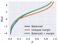
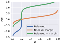
Figure 5: Comparison of link functions for various losses assuming $\pi=0.2$, with $\gamma=1$ (left) and $\gamma=8$ (right). The balanced loss uses $\omega_{y}=\frac{1}{\pi_{y}}$. The unequal margin loss uses $\delta_{y}=\frac{1}{\gamma}\cdot\log\frac{1-\pi}{\pi}$. The balanced + margin loss uses $\delta_{-1}=\frac{\pi}{1-\pi}$, $\delta_{+1}=1$, $\omega_{+1}=\frac{1}{\pi}$.

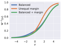
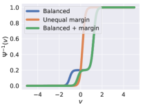
Figure 6: Comparison of link functions for various losses assuming $\pi=0.2$, with $\gamma=1$ (left) and $\gamma=8$ (right). The balanced loss uses $\omega_{y}=\frac{1}{\pi_{y}}$. The unequal margin loss uses $\delta_{y}=\frac{1}{\gamma}\cdot\log\frac{1-\pi_{y}}{\pi_{y}}$. The balanced + margin loss uses $\delta_{-1}=\frac{\pi}{1-\pi}$, $\delta_{+1}=1$, $\omega_{+1}=\frac{1}{\pi}$.

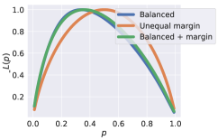
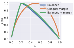
Figure 7: Comparison of conditional Bayes risk functions for various losses assuming $\pi=0.2$, with $\gamma=1$ (left) and $\gamma=8$ (right). The balanced loss uses $\omega_{y}=\frac{1}{\pi_{y}}$. The unequal margin loss uses $\delta_{y}=\frac{1}{\gamma}\cdot\log\frac{1-\pi_{y}}{\pi_{y}}$. The first balanced + margin loss uses $\delta_{-1}=\pi$, $\delta_{+1}=1$, $\omega_{+1}=\frac{1}{\pi}$. The second balanced + margin loss uses $\delta_{-1}=\frac{\pi}{1-\pi}$, $\delta_{+1}=1$, $\omega_{+1}=\frac{1}{\pi}$.

Appendix C Relation to cost-sensitive SVMs

We recapitulate the analysis of Masnadi-Shirazi and Vasconcelos [2010] in our notation. Consider a binary cost-sensitive learning problem with cost parameter $c\in(0,1)$. The Bayes-optimal classifier for this task corresponds to $f^{*}(x)=\llbracket\eta(x)>c\rrbracket$. The case $c=0.5$ is the standard classification problem.

Suppose we wish to design a weighted, variable margin SVM for this task, i.e.,

$$\ell(+1,f) ={\omega_{+1}}\cdot[\delta_{+1}-f]_{+}$$

$$\ell(-1,f) ={\omega_{-1}}\cdot[\delta_{-1}+f]_{+}$$

where $\omega_{\pm 1},\delta_{\pm 1}\geq 0$. The conditional risk for this loss is

$$L(\eta,f) =\eta\cdot\ell(+1,f)+(1-\eta)\cdot\ell(-1,f)$$

$$=\begin{cases}(1-\eta)\cdot{\omega_{-1}}\cdot(\delta_{-1}+f)&\text{ if }f>\delta_{+1}\\ \eta\cdot{\omega_{+1}}\cdot(\delta_{+1}-f)+(1-\eta)\cdot{\omega_{-1}}\cdot(\delta_{-1}+f)&\text{ if }f\in[-\delta_{-1},\delta_{+1}]\\ \eta\cdot{\omega_{+1}}\cdot(\delta_{+1}-f)&\text{ if }f<-\delta_{-1}.\end{cases}$$

As this is a piecewise linear function, which is decreasing for $f<-\delta_{-1}$ and increasing for $f>\delta_{+1}$, the only possible minimum is at $\{\delta_{+1},-\delta_{-1}\}$. To ensure consistency, we seek the minimum to be $\delta_{+1}$ iff $\eta>c$. Observe that

$$L(\eta,\delta_{+1})<L(\eta,-\delta_{-1}) \iff(1-\eta)\cdot{\omega_{-1}}<\eta\cdot\omega_{+1}$$

$$\iff\frac{\eta}{1-\eta}>\frac{\omega_{-1}}{\omega_{+1}}$$

$$\iff\eta>\frac{\omega_{-1}}{\omega_{-1}+\omega_{+1}}.$$

Consequently, we must have

$$\frac{\omega_{-1}}{\omega_{-1}+\omega_{+1}}=c\iff\frac{\omega_{+1}}{\omega_{-1}}=\frac{1-c}{c}.$$

Observe here that the margin terms $\delta_{\pm 1}$ do not appear in the consistency condition: thus, as long as the weights are suitably chosen, any choice of margin terms will result in a consistent loss.

However, the margins do influence the form conditional Bayes risk: this is

$$\underline{L}(\eta)=\begin{cases}(1-\eta)\cdot\omega_{-1}\cdot(\delta_{-1}+\delta_{+1})&\text{ if }\eta>c\\ \eta\cdot\omega_{-1}\cdot(\delta_{-1}+\delta_{+1})&\text{ if }\eta<c.\end{cases}$$

For the purposes of normalisation, it is natural to require this function to attain a maximum at $1$. This corresponds to choosing

$$\delta_{-1}+\delta_{+1}=\frac{1}{c}\cdot\frac{1}{\omega_{+1}}.$$

In the class-imbalance setting, $c=\pi$, and so we require

$$\frac{\omega_{+1}}{\omega_{-1}} =\frac{1-\pi}{\pi}$$

$$\delta_{-1}+\delta_{+1} =\frac{1}{\pi}\cdot\frac{1}{\omega_{+1}}$$

for consistency and normalisation respectively. This gives two degrees of freedom: the choice of $\omega_{+1}$ (which determines $\omega_{-1}$), and then the choice of $\delta_{+1}$ (which determines $\delta_{-1}$). For example, we could pick $\omega_{+1}=\frac{1}{\pi}$, $\omega_{-1}=\frac{1}{1-\pi}$, $\delta_{+1}=1$, $\delta_{-1}=\frac{\pi}{1-\pi}$.

To relate this to Masnadi-Shirazi and Vasconcelos [2010], the latter considered separate costs $C_{-1},C_{+1}$ for a false positive and false negative respectively. With this, they suggested to use Masnadi-Shirazi and Vasconcelos [2010, Equation 34]

$$\ell(+1,f) =d\cdot\left[\frac{e}{d}-f\right]_{+}$$

$$\ell(-1,f) =a\cdot\left[\frac{b}{a}+f\right]_{+}$$

with $\delta_{+1}=\frac{e}{d}=1$, $d=\omega_{+1}=C_{+1}$, $a=\omega_{-1}=2C_{-1}-1$, and $\delta_{-1}=\frac{b}{a}=\frac{1}{a}$. The constraints $C_{1}\geq 2C_{-1}-1$ and $C_{-1}\geq 1$ are also enforced.

Under this setup, the cost ratio is $\frac{C_{-1}}{C_{-1}+C_{+1}}$. In the class-imbalance setting, we have $\frac{C_{-1}}{C_{-1}+C_{+1}}=\pi$, and so $C_{+1}=\frac{1-\pi}{\pi}\cdot C_{-1}$. By the consistency condition, we have $C_{+1}=\omega_{+1}=\frac{1-\pi}{\pi}\cdot\omega_{-1}=\frac{1-\pi}{\pi}\cdot(2C_{-1}-1)$. Thus, we must set $C_{-1}=1$, and so $C_{+1}=\frac{1-\pi}{\pi}$. Thus, we obtain the parameters $\omega_{+1}=\frac{1-\pi}{\pi}$, $\omega_{-1}=1$, $\delta_{+1}=1$, $\delta_{-1}=\frac{\pi}{1-\pi}$. By rescaling the weights, we obtain $\omega_{+1}=\frac{1}{\pi}$, $\omega_{-1}=\frac{1}{1-\pi}$, $\delta_{+1}=1$, $\delta_{-1}=\frac{\pi}{1-\pi}$. Observe that this is exactly one of the losses considered in Appendix B.1.

Appendix D Experimental setup

Intending a fair comparison, we use the same setup for all the methods for each dataset. All networks are trained with SGD with a momentum value of 0.9. Unless otherwise specified, linear learning rate warm-up is used in the first 5 epochs to reach the base learning rate, and a weight decay of $10^{-4}$ is used. Other dataset specific details are given below.

CIFAR-10 and CIFAR-100: We use a CIFAR ResNet-32 model trained for 200 epochs. The base learning rate is set to 0.1, which is decayed by 0.1 at the 160th epoch and again at the 180th epoch. Mini-batches of 128 images are used.

We also use the standard CIFAR data augmentation procedure used in previous works such as Cao et al. [2019], He et al. [2016], where 4 pixels are padded on each size and a random $32\times 32$ crop is taken. Images are horizontally flipped with a probability of 0.5.

ImageNet: We use a ResNet-50 model trained for 90 epochs. The base learning rate is 0.4, with cosine learning rate decay. We use a batch size of 512 and the standard data augmentation comprising of random cropping and flipping as described in Goyal et al. [2017]. Following Kang et al. [2020], we use a weight decay of $5\times 10^{-4}$ on this dataset.

iNaturalist: We again use a ResNet-50 and train it for 90 epochs with a base learning rate of 0.4 and cosine learning rate decay. The data augmentation procedure is the same as the one used in ImageNet experiment above. We use a batch size of $512$.

Appendix E Additional experiments

We present here additional experiments:

1. we present results for CIFAR-10 and CIFAR-100 on the Step profile [Cao et al., 2019] with $\rho=100$

2. we further verfiy that weight norms may not correlate with class priors under Adam

3. we include the results of post-hoc correction, and a breakdown of per-class errors, on ImageNet-LT

E.1 Results on CIFAR-LT with Step-100 profile

Table 5 summarises results on the Step-100 profile. Here, with $\tau=1$, weight normalisation slightly outperforms logit adjustment. However, with $\tau>1$, logit adjustment is again found to be superior (54.80); see Figure 8.

Method	CIFAR-10-LT	CIFAR-100-LT
ERM	36.54	60.23
Weight normalisation ($\tau=1$)	30.86	55.19
Adaptive	34.61	58.86
Equalised	31.42	57.82
Logit adjustment post-hoc ($\tau=1$)	28.66	55.82
Logit adjustment (loss)	27.57	55.52

Table 5: Test set balanced error (averaged over $5$ trials) on CIFAR-10-LT and CIFAR-100-LT under the Step-100 profile; lower is better. On CIFAR-100-LT, weight normalisation edges out logit adjustment. See Figure 8 for a demonstrated that tuned versions of the same outperfom weight normalisation.

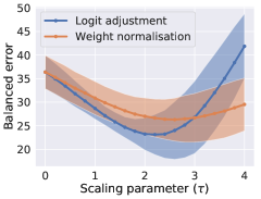
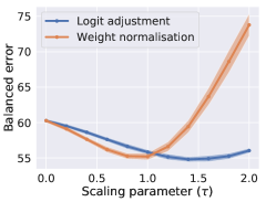
Figure 8: Post-hoc adjustment on Step-100 profile, CIFAR-10 and CIFAR-100. Logit adjustment outperforms weight normalisation with suitable tuning.

E.2 Per-class errors on ImageNet-LT

Figure 9 breaks down the per-class accuracies on ImageNet-LT. As before, the logit adjustment procedure shows significant gains on rarer classes.

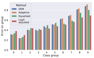
Figure 9: Comparison of per-class balanced error on ImageNet-LT. Classes are sorted in order of frequency, and bucketed into 10 groups.

E.3 Post-hoc correction on ImageNet-LT

Figure 10 compares post-hoc correction techniques as the scaling parameter $\tau$ is varied on ImageNet-LT. As before, logit adjustment with suitable tuning is seen to be competitive with weight normalisation.

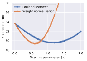
Figure 10: Post-hoc correction on ImageNet.

E.4 Per-group errors

Following Liu et al. [2019], Kang et al. [2020], we additionally report errors on a per-group basis, where we construct three groups of classes: “Many”, comprising those with at least 100 training examples; “Medium”, comprising those with at least 20 and at most 100 training examples; and “Few”, comprising those with at most 20 training examples. This is a coarser level of granularity than the grouping employed in the previous section, and the body. Figure 11 shows that the logit adjustment procedure shows consistent gains over all three groups.

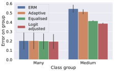
(a) CIFAR-10-LT

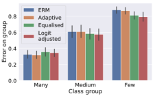
(b) CIFAR-100-LT.

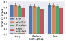
(c) ImageNet-LT.

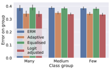
(d) iNaturalist.

Figure 11: Comparison of per-group errors. We construct three groups of classes: “Many”, comprising those with at least 100 training examples; “Medium”, comprising those with at least 20 and at most 100 training examples; and “Few”, comprising those with at most 20 training examples.

Appendix F Does weight normalisation increase margins?

Suppose that one uses SGD with a momentum, and finds solutions where $\|w_{y}\|_{2}$ tracks the class priors. One intuition behind normalisation of weights is that, drawing inspiration from the binary case, this ought to increase the classification margins for tail classes.

Unfortunately, this intuition is not necessarily borne out. Consider a scorer $f_{y}(x)=w_{y}^{\mathrm{T}}\Phi(x)$, where $w_{y}\in\mathbb{R}^{d}$ and $\Phi\colon\mathscr{X}\to\mathbb{R}^{d}$. The functional margin for an example $(x,y)$ is [Koltchinskii et al., 2001]

$$\gamma_{f}(x,y)\stackrel{{\scriptstyle.}}{{=}}w_{y}^{\mathrm{T}}\Phi(x)-\max_{y^{\prime}\neq y}w_{y^{\prime}}^{\mathrm{T}}\Phi(x).$$ (16)

This generalises the classical binary margin, wherein by convention $\mathscr{Y}=\{\pm 1\}$, $w_{-1}=-w_{1}$, and

$$\gamma_{\rm f}(x,y)\stackrel{{\scriptstyle.}}{{=}}y\cdot w_{1}^{\mathrm{T}}\Phi(x)={\frac{1}{2}}\cdot\left(w_{y}^{\mathrm{T}}\Phi(x)-w_{-y}^{\mathrm{T}}\Phi(x)\right),$$ (17)

which agrees with (16) upto scaling. One may also define the geometric margin in the binary case to be the distance of $(x,y)$ from its classifier:

$$\gamma_{g,{\rm b}}(x)\stackrel{{\scriptstyle.}}{{=}}\frac{|w_{1}\cdot\Phi(x)|}{\|w_{1}\|_{2}}.$$ (18)

Clearly, $\gamma_{g,{\rm b}}(x)=\frac{|\gamma_{\rm f}(x,y)|}{\|w_{1}\|_{2}}$, and so for fixed functional margin, one may increase the geometric margin by minimising $\|w_{1}\|_{2}$. However, the same is not necessarily true in the multiclass setting, since here the functional and geometric margins do not generally align [Tatsumi et al., 2011, Tatsumi and Tanino, 2014]. In particular, controlling each $\|w_{y}\|_{2}$ does not necessarily control the geometric margin.

Appendix G Bayes-optimal classifier under Gaussian class-conditionals

Suppose

$$\mathbb{P}(x\mid y)=\frac{1}{\sqrt{2\pi}\sigma}\cdot\exp\left(-\frac{\|x-\mu_{y}\|^{2}}{2\sigma^{2}}\right)$$

for suitable $\mu_{y}$ and $\sigma$. Then,

$$\mathbb{P}(x\mid y=+1)>\mathbb{P}(x\mid y=-1) \iff\exp\left(-\frac{\|x-\mu_{+1}\|^{2}}{2\sigma^{2}}\right)>\exp\left(-\frac{\|x-\mu_{-1}\|^{2}}{2\sigma^{2}}\right)$$

$$\iff\frac{\|x-\mu_{+1}\|^{2}}{2\sigma^{2}}<\frac{\|x-\mu_{-1}\|^{2}}{2\sigma^{2}}$$

$$\iff{\|x-\mu_{+1}\|^{2}}<{\|x-\mu_{-1}\|^{2}}$$

$$\iff 2\cdot(\mu_{+1}-\mu_{-1})^{\mathrm{T}}x>\|\mu_{+1}\|^{2}-\|\mu_{-1}\|^{2}.$$

Now use the fact that in our setting, $\|\mu_{+1}\|^{2}=\|\mu_{-1}\|^{2}$.

We remark also that the class-probability function is

$$\mathbb{P}(y=+1\mid x) =\frac{\mathbb{P}(x\mid y=+1)\cdot\mathbb{P}(y=+1)}{\mathbb{P}(x)}$$

$$=\frac{\mathbb{P}(x\mid y=+1)\cdot\mathbb{P}(y=+1)}{\sum_{y^{\prime}}\mathbb{P}(x\mid y^{\prime})\cdot\mathbb{P}(y^{\prime})}$$

$$=\frac{1}{1+\frac{\mathbb{P}(x\mid y=-1)\cdot\mathbb{P}(y=-1)}{\mathbb{P}(x\mid y=+1)\cdot\mathbb{P}(y=+1)}}.$$

Now,

$$\frac{\mathbb{P}(x\mid y=-1)}{\mathbb{P}(x\mid y=+1)} =\exp\left(\frac{\|x-\mu_{+1}\|^{2}-\|x-\mu_{-1}\|^{2}}{2\sigma^{2}}\right)$$

$$=\exp\left(\frac{\|\mu_{+1}\|^{2}-\|\mu_{-1}\|^{2}-2\cdot(\mu_{+1}-\mu_{-1})^{\mathrm{T}}x}{2\sigma^{2}}\right)$$

$$=\exp\left(\frac{-(\mu_{+1}-\mu_{-1})^{\mathrm{T}}x}{\sigma^{2}}\right).$$

Thus,

$$\mathbb{P}(y=+1\mid x)=\frac{1}{1+\exp(-w_{*}^{\mathrm{T}}x+b_{*})},$$

where $w_{*}=\frac{1}{\sigma^{2}}\cdot(\mu_{+1}-\mu_{-1})$, and $b_{*}=\log\frac{\mathbb{P}(y=-1)}{\mathbb{P}(y=+1)}$. This implies that a sigmoid model for $\mathbb{P}(y=+1\mid x)$, as employed by logistic regression, is well-specified for the problem. Further, the bias term $b_{*}$ is seen to take the form of the log-odds of the class-priors per (8), as expected.

References

- Bartlett et al. [2006] Peter L. Bartlett, Michael I. Jordan, and Jon D. McAuliffe. Convexity, classification, and risk bounds. Journal of the American Statistical Association, 101(473):138–156, 2006.
- Bengio and Senecal [2008] Y. Bengio and J. S. Senecal. Adaptive importance sampling to accelerate training of a neural probabilistic language model. Trans. Neur. Netw., 19(4):713–722, April 2008. ISSN 1045-9227.
- Brodersen et al. [2010] Kay H. Brodersen, Cheng Soon Ong, Klaas E. Stephan, and Joachim M. Buhmann. The balanced accuracy and its posterior distribution. In Proceedings of the International Conference on Pattern Recognition (ICPR), pages 3121–3124, Aug 2010.
- Buda et al. [2017] Mateusz Buda, Atsuto Maki, and Maciej A. Mazurowski. A systematic study of the class imbalance problem in convolutional neural networks. arXiv:1710.05381 [cs, stat], October 2017.
- Byrd and Lipton [2019] Jonathon Byrd and Zachary Chase Lipton. What is the effect of importance weighting in deep learning? In Proceedings of the 36th International Conference on Machine Learning, ICML 2019, 9-15 June 2019, Long Beach, California, USA, pages 872–881, 2019.
- Cao et al. [2019] Kaidi Cao, Colin Wei, Adrien Gaidon, Nikos Arechiga, and Tengyu Ma. Learning imbalanced datasets with label-distribution-aware margin loss. In Advances in Neural Information Processing Systems, 2019.
- Cardie and Howe [1997] Claire Cardie and Nicholas Howe. Improving minority class prediction using case-specific feature weights. In Proceedings of the International Conference on Machine Learning (ICML), 1997.
- Chan and Stolfo [1998] Philip K. Chan and Salvatore J. Stolfo. Learning with non-uniform class and cost distributions: Effects and a distributed multi-classifier approach. In KDD-98 Workshop on Distributed Data Mining, 1998.
- Chawla et al. [2002] Nitesh V. Chawla, Kevin W. Bowyer, Lawrence O. Hall, and W. Philip Kegelmeyer. SMOTE: Synthetic minority over-sampling technique. Journal of Artificial Intelligence Research (JAIR), 16:321–357, 2002.
- Collell et al. [2016] Guillem Collell, Drazen Prelec, and Kaustubh R. Patil. Reviving threshold-moving: a simple plug-in bagging ensemble for binary and multiclass imbalanced data. CoRR, abs/1606.08698, 2016.
- Cui et al. [2019] Yin Cui, Menglin Jia, Tsung-Yi Lin, Yang Song, and Serge Belongie. Class-balanced loss based on effective number of samples. In CVPR, 2019.
- Dmochowski et al. [2010] Jacek P. Dmochowski, Paul Sajda, and Lucas C. Parra. Maximum likelihood in cost-sensitive learning: Model specification, approximations, and upper bounds. Journal of Machine Learning Research, 11:3313–3332, 2010.
- Elkan [2001] Charles Elkan. The foundations of cost-sensitive learning. In Proceedings of the International Joint Conference on Artificial Intelligence (IJCAI), 2001.
- Fan et al. [2017] Yanbo Fan, Siwei Lyu, Yiming Ying, and Baogang Hu. Learning with average top-k loss. In I. Guyon, U. V. Luxburg, S. Bengio, H. Wallach, R. Fergus, S. Vishwanathan, and R. Garnett, editors, Advances in Neural Information Processing Systems 30, pages 497–505. Curran Associates, Inc., 2017.
- Fawcett and Provost [1996] Tom Fawcett and Foster Provost. Combining data mining and machine learning for effective user profiling. In Proceedings of the ACM SIGKDD International Conference on Knowledge Discovery and Data Mining (KDD), pages 8–13. AAAI Press, 1996.
- Gneiting and Raftery [2007] Tilmann Gneiting and Adrian E Raftery. Strictly proper scoring rules, prediction, and estimation. Journal of the American Statistical Association, 102(477):359–378, 2007.
- Gneiting et al. [2007] Tilmann Gneiting, Fadoua Balabdaoui, and Adrian E. Raftery. Probabilistic forecasts, calibration and sharpness. Journal of the Royal Statistical Society: Series B (Statistical Methodology), 69(2):243–268, 2007.
- Gottlieb et al. [2020] Lee-Ad Gottlieb, Eran Kaufman, and Aryeh Kontorovich. Apportioned margin approach for cost sensitive large margin classifiers, 2020.
- Goyal et al. [2017] Priya Goyal, Piotr Dollár, Ross Girshick, Pieter Noordhuis, Lukasz Wesolowski, Aapo Kyrola, Andrew Tulloch, Yangqing Jia, and Kaiming He. Accurate, large minibatch sgd: Training imagenet in 1 hour. arXiv preprint arXiv:1706.02677, 2017.
- Guo et al. [2017] Chuan Guo, Geoff Pleiss, Yu Sun, and Kilian Q. Weinberger. On calibration of modern neural networks. In Proceedings of the 34th International Conference on Machine Learning, ICML 2017, Sydney, NSW, Australia, 6-11 August 2017, pages 1321–1330, 2017.
- Hazan and Urtasun [2010] Tamir Hazan and Raquel Urtasun. Approximated structured prediction for learning large scale graphical models. CoRR, abs/1006.2899, 2010. URL http://arxiv.org/abs/1006.2899.
- He and Garcia [2009] Haibo He and Edwardo A. Garcia. Learning from imbalanced data. IEEE Transactions on Knowledge and Data Engineering, 21(9):1263–1284, 2009.
- He et al. [2016] K. He, X. Zhang, S. Ren, and J. Sun. Deep residual learning for image recognition. In 2016 IEEE Conference on Computer Vision and Pattern Recognition (CVPR), 2016.
- Hinton et al. [2015] Geoffrey E. Hinton, Oriol Vinyals, and Jeffrey Dean. Distilling the knowledge in a neural network. CoRR, abs/1503.02531, 2015.
- Iranmehr et al. [2019] Arya Iranmehr, Hamed Masnadi-Shirazi, and Nuno Vasconcelos. Cost-sensitive support vector machines. Neurocomputing, 343:50–64, 2019.
- Jamal et al. [2020] Muhammad Abdullah Jamal, Matthew Brown, Ming-Hsuan Yang, Liqiang Wang, and Boqing Gong. Rethinking class-balanced methods for long-tailed visual recognition from a domain adaptation perspective, 2020.
- Kang et al. [2020] Bingyi Kang, Saining Xie, Marcus Rohrbach, Zhicheng Yan, Albert Gordo, Jiashi Feng, and Yannis Kalantidis. Decoupling representation and classifier for long-tailed recognition. In Eighth International Conference on Learning Representations (ICLR), 2020.
- Khan et al. [2019] S. Khan, M. Hayat, S. W. Zamir, J. Shen, and L. Shao. Striking the right balance with uncertainty. In 2019 IEEE/CVF Conference on Computer Vision and Pattern Recognition (CVPR), pages 103–112, 2019.
- Kim and Kim [2019] Byungju Kim and Junmo Kim. Adjusting decision boundary for class imbalanced learning, 2019.
- King and Zeng [2001] Gary King and Langche Zeng. Logistic regression in rare events data. Political Analysis, 9(2):137–163, 2001.
- Koltchinskii et al. [2001] Vladimir Koltchinskii, Dmitriy Panchenko, and Fernando Lozano. Some new bounds on the generalization error of combined classifiers. In T. K. Leen, T. G. Dietterich, and V. Tresp, editors, Advances in Neural Information Processing Systems 13, pages 245–251. MIT Press, 2001.
- Kubat and Matwin [1997] Miroslav Kubat and Stan Matwin. Addressing the curse of imbalanced training sets: One-sided selection. In Proceedings of the International Conference on Machine Learning (ICML), 1997.
- Kuleshov et al. [2018] Volodymyr Kuleshov, Nathan Fenner, and Stefano Ermon. Accurate uncertainties for deep learning using calibrated regression. In Jennifer Dy and Andreas Krause, editors, Proceedings of the 35th International Conference on Machine Learning, volume 80 of Proceedings of Machine Learning Research, pages 2796–2804, Stockholmsmässan, Stockholm Sweden, 10–15 Jul 2018. PMLR.
- Li et al. [2002] Yaoyong Li, Hugo Zaragoza, Ralf Herbrich, John Shawe-Taylor, and Jaz S. Kandola. The perceptron algorithm with uneven margins. In Proceedings of the Nineteenth International Conference on Machine Learning, ICML ’02, page 379–386, San Francisco, CA, USA, 2002. Morgan Kaufmann Publishers Inc. ISBN 1558608737.
- Lin [2004] Yi Lin. A note on margin-based loss functions in classification. Statistics & Probability Letters, 68(1):73 – 82, 2004. ISSN 0167-7152.
- Liu et al. [2016] Weiyang Liu, Yandong Wen, Zhiding Yu, and Meng Yang. Large-margin softmax loss for convolutional neural networks. In Proceedings of the 33rd International Conference on International Conference on Machine Learning - Volume 48, ICML’16, page 507–516. JMLR.org, 2016.
- Liu et al. [2017] Weiyang Liu, Yandong Wen, Zhiding Yu, Ming Li, Bhiksha Raj, and Le Song. Sphereface: Deep hypersphere embedding for face recognition. In 2017 IEEE Conference on Computer Vision and Pattern Recognition, CVPR 2017, Honolulu, HI, USA, July 21-26, 2017, pages 6738–6746, 2017.
- Liu et al. [2019] Ziwei Liu, Zhongqi Miao, Xiaohang Zhan, Jiayun Wang, Boqing Gong, and Stella X. Yu. Large-scale long-tailed recognition in an open world. In IEEE Conference on Computer Vision and Pattern Recognition, CVPR 2019, Long Beach, CA, USA, June 16-20, 2019, pages 2537–2546. Computer Vision Foundation / IEEE, 2019.
- Mahajan et al. [2018] Dhruv Mahajan, Ross Girshick, Vignesh Ramanathan, Kaiming He, Manohar Paluri, Yixuan Li, Ashwin Bharambe, and Laurens van der Maaten. Exploring the limits of weakly supervised pretraining. In Vittorio Ferrari, Martial Hebert, Cristian Sminchisescu, and Yair Weiss, editors, Computer Vision – ECCV 2018, pages 185–201, Cham, 2018. Springer International Publishing. ISBN 978-3-030-01216-8.
- Maloof [2003] Marcus A. Maloof. Learning when data sets are imbalanced and when costs are unequal and unknown. In ICML 2003 Workshop on Learning from Imbalanced Datasets, 2003.
- Masnadi-Shirazi and Vasconcelos [2010] Hamed Masnadi-Shirazi and Nuno Vasconcelos. Risk minimization, probability elicitation, and cost-sensitive SVMs. In Proceedings of the 27th International Conference on International Conference on Machine Learning, ICML’10, page 759–766, Madison, WI, USA, 2010. Omnipress. ISBN 9781605589077.
- Menon et al. [2013] Aditya Krishna Menon, Harikrishna Narasimhan, Shivani Agarwal, and Sanjay Chawla. On the statistical consistency of algorithms for binary classification under class imbalance. In Proceedings of the 30th International Conference on Machine Learning, ICML 2013, Atlanta, GA, USA, 16-21 June 2013, pages 603–611, 2013.
- Mikolov et al. [2013] Tomas Mikolov, Ilya Sutskever, Kai Chen, Greg Corrado, and Jeffrey Dean. Distributed representations of words and phrases and their compositionality. In Proceedings of the 26th International Conference on Neural Information Processing Systems, NIPS’13, page 3111–3119, Red Hook, NY, USA, 2013. Curran Associates Inc.
- Morik et al. [1999] Katharina Morik, Peter Brockhausen, and Thorsten Joachims. Combining statistical learning with a knowledge-based approach - a case study in intensive care monitoring. In Proceedings of the Sixteenth International Conference on Machine Learning (ICML), pages 268–277, San Francisco, CA, USA, 1999. Morgan Kaufmann Publishers Inc. ISBN 1-55860-612-2.
- Müller et al. [2019] Rafael Müller, Simon Kornblith, and Geoffrey E. Hinton. When does label smoothing help? In Advances in Neural Information Processing Systems 32: Annual Conference on Neural Information Processing Systems 2019, NeurIPS 2019, 8-14 December 2019, Vancouver, BC, Canada, pages 4696–4705, 2019.
- Murphy and Winkler [1987] Allan H. Murphy and Robert L. Winkler. A general framework for forecast verification. Monthly Weather Review, 115(7):1330–1338, 1987.
- Pletscher et al. [2010] Patrick Pletscher, Cheng Soon Ong, and Joachim M. Buhmann. Entropy and margin maximization for structured output learning. In José Luis Balcázar, Francesco Bonchi, Aristides Gionis, and Michèle Sebag, editors, Machine Learning and Knowledge Discovery in Databases, pages 83–98, Berlin, Heidelberg, 2010. Springer Berlin Heidelberg.
- Provost [2000] Foster Provost. Machine learning from imbalanced data sets 101. In Proceedings of the AAAI-2000 Workshop on Imbalanced Data Sets, 2000.
- Qiao and Liu [2009] Xingye Qiao and Yufeng Liu. Adaptive weighted learning for unbalanced multicategory classification. Biometrics, 65(1):159–168, 2009.
- Reid and Williamson [2010] Mark D. Reid and Robert C. Williamson. Composite binary losses. Journal of Machine Learning Research, 11:2387–2422, 2010.
- Soudry et al. [2018] Daniel Soudry, Elad Hoffer, Mor Shpigel Nacson, Suriya Gunasekar, and Nathan Srebro. The implicit bias of gradient descent on separable data. J. Mach. Learn. Res., 19(1):2822–2878, January 2018. ISSN 1532-4435.
- Szegedy et al. [2016] Christian Szegedy, Vincent Vanhoucke, Sergey Ioffe, Jonathon Shlens, and Zbigniew Wojna. Rethinking the inception architecture for computer vision. In 2016 IEEE Conference on Computer Vision and Pattern Recognition, CVPR 2016, Las Vegas, NV, USA, June 27-30, 2016, pages 2818–2826, 2016.
- Tan et al. [2020] Jingru Tan, Changbao Wang, Buyu Li, Quanquan Li, Wanli Ouyang, Changqing Yin, and Junjie Yan. Equalization loss for long-tailed object recognition, 2020.
- Tatsumi and Tanino [2014] Keiji Tatsumi and Tetsuzo Tanino. Support vector machines maximizing geometric margins for multi-class classification. TOP, 22(3):815–840, 2014.
- Tatsumi et al. [2011] Keiji Tatsumi, Masashi Akao, Ryo Kawachi, and Tetsuzo Tanino. Performance evaluation of multiobjective multiclass support vector machines maximizing geometric margins. Numerical Algebra, Control & Optimization, 1:151, 2011. ISSN 2155-3289.
- Van Horn and Perona [2017] Grant Van Horn and Pietro Perona. The devil is in the tails: Fine-grained classification in the wild. arXiv preprint arXiv:1709.01450, 2017.
- Wallace et al. [2011] B.C. Wallace, K.Small, C.E. Brodley, and T.A. Trikalinos. Class imbalance, redux. In Proc. ICDM, 2011.
- Wang et al. [2018] F. Wang, J. Cheng, W. Liu, and H. Liu. Additive margin softmax for face verification. IEEE Signal Processing Letters, 25(7):926–930, 2018.
- Wu et al. [2008] Shan-Hung Wu, Keng-Pei Lin, Chung-Min Chen, and Ming-Syan Chen. Asymmetric support vector machines: Low false-positive learning under the user tolerance. In Proceedings of the 14th ACM SIGKDD International Conference on Knowledge Discovery and Data Mining, KDD ’08, page 749–757, New York, NY, USA, 2008. Association for Computing Machinery. ISBN 9781605581934.
- Xie and Manski [1989] Yu Xie and Charles F. Manski. The logit model and response-based samples. Sociological Methods & Research, 17(3):283–302, 1989.
- Ye et al. [2020] Han-Jia Ye, Hong-You Chen, De-Chuan Zhan, and Wei-Lun Chao. Identifying and compensating for feature deviation in imbalanced deep learning, 2020.
- Yi et al. [2019] Xinyang Yi, Ji Yang, Lichan Hong, Derek Zhiyuan Cheng, Lukasz Heldt, Aditee Kumthekar, Zhe Zhao, Li Wei, and Ed Chi. Sampling-bias-corrected neural modeling for large corpus item recommendations. In Proceedings of the 13th ACM Conference on Recommender Systems, RecSys ’19, page 269–277, New York, NY, USA, 2019. Association for Computing Machinery. ISBN 9781450362436.
- Yin et al. [2018] Xi Yin, Xiang Yu, Kihyuk Sohn, Xiaoming Liu, and Manmohan Chandraker. Feature transfer learning for deep face recognition with long-tail data. CoRR, abs/1803.09014, 2018.
- Zadrozny and Elkan [2001] Bianca Zadrozny and Charles Elkan. Learning and making decisions when costs and probabilities are both unknown. In Proceedings of the Seventh ACM SIGKDD International Conference on Knowledge Discovery and Data Mining, KDD ’01, page 204–213, New York, NY, USA, 2001. Association for Computing Machinery. ISBN 158113391X.
- Zhang et al. [2019] Junjie Zhang, Lingqiao Liu, Peng Wang, and Chunhua Shen. To balance or not to balance: A simple-yet-effective approach for learning with long-tailed distributions, 2019.
- Zhang [2004] Tong Zhang. Class-size independent generalization analsysis of some discriminative multi-category classification methods. In Proceedings of the 17th International Conference on Neural Information Processing Systems, NIPS’04, page 1625–1632, Cambridge, MA, USA, 2004. MIT Press.
- Zhang et al. [2017] X. Zhang, Z. Fang, Y. Wen, Z. Li, and Y. Qiao. Range loss for deep face recognition with long-tailed training data. In 2017 IEEE International Conference on Computer Vision (ICCV), pages 5419–5428, 2017.
- Zhou and Liu [2006] Zhi-Hua Zhou and Xu-Ying Liu. Training cost-sensitive neural networks with methods addressing the class imbalance problem. IEEE Transactions on Knowledge and Data Engineering (TKDE), 18(1), 2006.