Momentum-Based Policy Gradient Methods

Abstract

In the paper, we propose a class of efficient momentum-based policy gradient methods for the model-free reinforcement learning, which use adaptive learning rates and do not require any large batches. Specifically, we propose a fast important-sampling momentum-based policy gradient (IS-MBPG) method based on a new momentum-based variance reduced technique and the importance sampling technique. We also propose a fast Hessian-aided momentum-based policy gradient (HA-MBPG) method based on the momentum-based variance reduced technique and the Hessian-aided technique. Moreover, we prove that both the IS-MBPG and HA-MBPG methods reach the best known sample complexity of $O(\epsilon^{-3})$ for finding an $\epsilon$-stationary point of the nonconcave performance function, which only require one trajectory at each iteration. In particular, we present a non-adaptive version of IS-MBPG method, i.e., IS-MBPG*, which also reaches the best known sample complexity of $O(\epsilon^{-3})$ without any large batches. In the experiments, we apply four benchmark tasks to demonstrate the effectiveness of our algorithms.

1 Introduction

Reinforcement Learning (RL) has achieved great success in solving many sequential decision-making problems such as autonomous driving (Shalev-Shwartz et al., 2016), robot manipulation (Deisenroth et al., 2013), the game of Go (Silver et al., 2017) and natural language processing (Wang et al., 2018). In general, RL involves a Markov decision process (MDP), where an agent takes actions dictated by a policy in a stochastic environment over a sequence of time steps, and then maximizes the long-term cumulative rewards to obtain an optimal policy. Due to easy implementation and avoiding policy degradation, policy gradient method (Williams, 1992; Sutton et al., 2000) is widely used for finding the optimal policy in MDPs, especially for the high dimensional continuous state and action spaces. To obtain the optimal policy, policy gradient methods directly maximize the expected total reward (also called as performance function $J(\theta)$) via using the stochastic first-order gradient of cumulative rewards. Recently, policy gradient methods have achieved significant empirical successes in many challenging deep reinforcement learning applications (Li, 2017) such as playing game of Go and robot manipulation.

Table 1: Convergence properties of the representative variance-reduced policy algorithms on the non-oblivious model-free RL problem for finding an $\epsilon$-stationary point of the nonconcave performance function $J(\theta)$, i.e., $\mathbb{E}\|\nabla J(\theta)\|\leq\epsilon$. Our algorithms (IS-MBPG, IS-MBPG* and HA-MBPG) and REINFORCE are single-loop algorithms, while the other algorithms are double-loops, which need the outer-loop and inner-loop mini-batch sizes. Note that Papini et al. (2018) only remarked that apply the ADAM algorithm (Kingma & Ba, 2014) to the SVRPG algorithm to obtain an adaptive learning rate, but did not provide any theoretical analysis about this learning rate. In addition, the sample complexity $O(\epsilon^{-4})$ of REINFORCE does not directly come from (Williams, 1992), but follows theoretical results of SGD (Ghadimi & Lan, 2013) (A detailed theoretical analysis is given in the Appendix A.4).

Algorithm	Reference	Sample Complexity	Batch Size	Adaptive Learning Rate
REINFORCE	Williams (1992)	$O(\epsilon^{-4})$	$O(\epsilon^{-2})$
SVRPG	Papini et al. (2018)	$O(\epsilon^{-4})$	$O(\epsilon^{-2})$ & $O(\epsilon^{-2})$
SVRPG	Xu et al. (2019a)	$O(\epsilon^{-10/3})$	$O(\epsilon^{-4/3})$ & $O(\epsilon^{-2})$
HAPG	Shen et al. (2019)	$O(\epsilon^{-3})$	$O(\epsilon^{-1})$ & $O(\epsilon^{-2})$
SRVR-PG	Xu et al. (2019b)	$O(\epsilon^{-3})$	$O(\epsilon^{-1})$ & $O(\epsilon^{-2})$
IS-MBPG	Ours	$O(\epsilon^{-3})$	$O(1)$	✓
HA-MBPG	Ours	$O(\epsilon^{-3})$	$O(1)$	✓
IS-MBPG*	Ours	$O(\epsilon^{-3})$	$O(1)$

Thus, policy gradient methods have regained much interest in reinforcement learning, and some corresponding algorithms and theory of policy gradient (Fellows et al., 2018; Fujimoto et al., 2018; Papini et al., 2018; Haarnoja et al., 2018; Xu et al., 2019a; Shen et al., 2019; Cheng et al., 2019b, a; Wang et al., 2019a) have been proposed and studied. Since the classic policy gradient methods (e.g., REINFORCE (Williams, 1992), PGT (Sutton et al., 2000), GPOMDP (Baxter & Bartlett, 2001) and TRPO (Schulman et al., 2015a)) approximate the gradient of the expected total reward based on a batch of sampled trajectories, they generally suffer from large variance in the estimated gradients, which results in a poor convergence. Following the standard stochastic gradient methods (Robbins & Monro, 1951; Ghadimi & Lan, 2013), these gradient-based policy methods require $O(\epsilon^{-4})$ samples for finding an $\epsilon$-stationary point of non-concave performance function $J(\theta)$ ( i.e., $\mathbb{E}\|\nabla J(\theta)\|\leq\epsilon$). Thus, recently many works have begun to study to reduce variance in the policy gradient methods. For example, the early variance reduced policy methods (Greensmith et al., 2004; Peters & Schaal, 2008) mainly focused on using unbiased baseline functions to reduce the variance. Schulman et al. (2015b) presented the generalized advantage estimation (GAE) to discover the balance between bias and variance of policy gradient. Then Gu et al. (2016) applied both the GAE and linear baseline function to reduce variance. Recently, Mao et al. (2018); Wu et al. (2018) proposed the input-dependent and action-dependent baselines to reduce the variance, respectively. More recently, Cheng et al. (2019b) leveraged the predictive models to reduce the variance to accelerate policy learning.

Recently, the variance reduced gradient estimators such as SVRG (Johnson & Zhang, 2013; Allen-Zhu & Hazan, 2016; Reddi et al., 2016), SAGA (Defazio et al., 2014), SARAH (Nguyen et al., 2017), SPIDER (Fang et al., 2018), SpiderBoost (Wang et al., 2019b) and SNVRG (Zhou et al., 2018) have been successful in the oblivious supervised learning. However, the RL optimization problems are non-oblivious, i.e., the distribution of the samples is non-stationarity and changes over time. Thus, Du et al. (2017); Xu et al. (2017); Wai et al. (2019) first transform the original non-oblivious policy evaluation problem into some oblivious subproblems, and then use the existing variance reduced gradient estimators (such as SVRG and SAGA) to solve these subproblems to reach the goal of reducing the large variance in the original RL problem. For example, Du et al. (2017) first transforms the empirical policy evaluation problem into a quadratic convex-concave saddle-point problem via linear function approximation, and then applies the variants of SVRG and SAGA (Palaniappan & Bach, 2016) to solve this oblivious saddle-point problem.

More recently, Papini et al. (2018); Xu et al. (2019a, b); Shen et al. (2019) further have developed some variance reduced policy gradient estimators directly used in the non-oblivious model-free RL, based on the existing variance reduced techniques such as SVRG and SPIDER used in the oblivious supervised learning. Moreover, Xu et al. (2019a, b); Shen et al. (2019) have effectively improved the sample complexity by using these variance reduced policy gradients. For example, two efficient variance reduced policy gradient methods, i.e, SRVR-PG (Xu et al., 2019b) and HAPG (Shen et al., 2019) have been proposed based on the SARAH/SPIDER, and reach a sharp sample complexity of $O(\epsilon^{-3})$ for finding an $\epsilon$-stationary point, which improves the vanilla complexity of $O(\epsilon^{-4})$ (Williams, 1992) by a factor of $O(\epsilon^{-1})$. Since a lower bound of complexity of $O(\epsilon^{-3})$ for recently proposed variance reduction techniques is established in (Arjevani et al., 2019), both the SRVR-PG and HAPG obtain a near-optimal sample complexity of $O(\epsilon^{-3})$. However, the practical performances of these variance reduced policy gradient methods are not consistent with their near-optimal sample complexity, because these methods require large batches and strict learning rates to achieve this optimal complexity.

In the paper, thus, we propose a class of efficient momentum-based policy gradient methods, which use adaptive learning rates and do not require any large batches. Specifically, our algorithms only need one trajectory at each iteration, and use adaptive learning rates based on the current and historical stochastic gradients. Note that Pirotta et al. (2013) has studied the adaptive learning rates for policy gradient methods, which only focuses on Gaussian policy. Moreover, Pirotta et al. (2013) did not consider sample complexity and can not improve it. While our algorithms not only provide the adaptive learning rates that are suitable for any policies, but also improve sample complexity.

Contributions

Our main contributions are summarized as follows:

• We propose a fast important-sampling momentum-based policy gradient (IS-MBPG) method with adaptive learning rate, which builds on a new momentum-based variance reduction technique of STORM/Hybrid-SGD (Cutkosky & Orabona, 2019; Tran-Dinh et al., 2019) and the importance sampling technique.

• We propose a fast Hessian-aided momentum-based policy gradient (HA-MBPG) method with adaptive learning rate, based on the momentum-based variance reduction technique and the Hessian-aided technique.

• We study the sample complexity of our methods, and prove that both the IS-MBPG and HA-MBPG methods reach the best known sample complexity of $O(\epsilon^{-3})$ without any large batches (see Table 1).

• We propose a non-adaptive version of IS-MBPG method, i.e., IS-MBPG*, which has a simple monotonically decreasing learning rate. We prove that it also reaches the best known sample complexity of $O(\epsilon^{-3})$ without any large batches.

After our paper is accepted, we find that three related papers (Xiong et al., 2020; Pham et al., 2020; Yuan et al., 2020) more recently are released on arXiv. Xiong et al. (2020) has studied the adaptive Adam-type policy gradient (PG-AMSGrad) method, which still suffers from a high sample complexity of $O(\epsilon^{-4})$. Subsequently, Pham et al. (2020); Yuan et al. (2020) have proposed the policy gradient methods, i.e., ProxHSPGA and STORM-PG, respectively, which also build on the momentum-based variance reduced technique of STORM/Hybrid-SGD. Although both the ProxHSPGA and STORM-PG reach the best known sample complexity of $O(\epsilon^{-3})$, these methods still rely on large batch sizes to obtain this sample complexity and do not provide an effective adaptive learning rate as our methods.

Notations

Let $\|\cdot\|$ denote the vector $\ell_{2}$ norm and the matrix spectral norm, respectively. We denote $a_{n}=O(b_{n})$ if $a_{n}\leq cb_{n}$ for some constant $c>0$. $\mathbb{E}[X]$ and $\mathbb{V}[X]$ denote the expectation and variance of a random variable $X$, respectively. $\mathbb{E}_{\tau_{t}}[\cdot]=\mathbb{E}_{\tau_{t}}[\cdot|\tau_{1},\cdots,\tau_{t-1}]$ for any $t\geq 2$.

2 Background

In the section, we will review some preliminaries of standard reinforcement learning and policy gradient.

2.1 Reinforcement Learning

Reinforcement learning is generally modeled as a discrete time Markov Decision Process (MDP): $\mathcal{M}=\{\mathcal{S},\mathcal{A},\mathcal{P},\mathcal{R},\gamma,\rho_{0}\}$. Here $\mathcal{S}$ is the state space, $\mathcal{A}$ is the action space, and $\rho_{0}$ denotes the initial state distribution. $\mathcal{P}(s^{\prime}|s,a)$ denotes the probability that the agent transits from the state $s$ to $s^{\prime}$ under taking the action $a\in\mathcal{A}$. $\mathcal{R}(s,a):\mathcal{S}\times\mathcal{A}\mapsto[-R,R]\ (R>0)$ is the bounded reward function, i.e., the agent obtain the reward $\mathcal{R}(s,a)$ after it takes the action $a$ at the state $s$, and $\gamma\in(0,1)$ is the discount factor. The policy $\pi(a|s)$ at the state $s$ is represented by a conditional probability distribution $\pi_{\theta}(a|s)$ associated to the parameter $\theta\in\mathbb{R}^{d}$.

Given a time horizon $H$, the agent can collect a trajectory $\tau=\{s_{0},a_{0},\cdots,s_{H-1},a_{H-1}\}$ under any stationary policy. Following the trajectory $\tau$, a cumulative discounted reward can be given as follows:

$$\mathcal{R}(\tau)=\sum^{H-1}_{h=0}\gamma^{h}\mathcal{R}(s_{h},a_{h}),$$ (1)

where $\gamma$ is the discount factor. Assume that the policy $\pi_{\theta}$ is parameterized by an unknown parameter $\theta\in\mathbb{R}^{d}$. Given the initial distribution $\rho_{0}=\rho(s_{0})$, the probability distribution over trajectory $\tau$ can be obtain

$$p(\tau|\theta)=\rho(s_{0})\prod_{h=0}^{H-1}\mathcal{P}(s_{h+1}|s_{h},a_{h})\pi_{\theta}(a_{h}|s_{h}).$$ (2)

2.2 Policy Gradient

The goal of RL is to find an optimal policy $\pi_{\theta}$ that is equivalent to maximize the expected discounted trajectory reward:

$$\max_{\theta\in\mathbb{R}^{d}}J(\theta):=\mathbb{E}_{\tau\sim p(\tau|\theta)}[\mathcal{R}(\tau)]=\int\mathcal{R}(\tau)p(\tau|\theta)d\tau.$$ (3)

Since the underlying distribution $p$ depends on the variable $\theta$ and varies through the whole optimization procedure, the problem (3) is a non-oblivious learning problem, which is unlike the traditional supervised learning problems that the underlying distribution $p$ is stationary. To deal with this problem, the policy gradient method (Williams, 1992; Sutton et al., 2000) is a good choice. Specifically, we first compute the gradient of $J(\theta)$ with respect to $\theta$, and obtain

$$\nabla J(\theta) \!=\!\int\!\mathcal{R}(\tau)\nabla p(\tau|\theta)d\tau\!=\!\int\!\mathcal{R}(\tau)\frac{\nabla p(\tau|\theta)}{p(\tau|\theta)}p(\tau|\theta)d\tau$$

$$\!=\mathbb{E}_{\tau\sim p(\tau|\theta)}\big{[}\nabla\log p(\tau|\theta)\mathcal{R}(\tau)\big{]}.$$ (4)

Since the distribution $p(\tau|\theta)$ is unknown, we can not compute the exact full gradient of (2.2). Similar for stochastic gradient descent (SGD), the policy gradient method samples a batch of trajectories $\mathcal{B}=\{\tau_{i}\}_{i=1}^{|\mathcal{B}|}$ from the distribution $p(\tau|\theta)$ to obtain the stochastic gradient as follows:

$$\hat{\nabla}J(\theta)=\frac{1}{|\mathcal{B}|}\sum_{i\in\mathcal{B}}\nabla\log p(\tau_{i}|\theta)\mathcal{R}(\tau_{i}).$$

At the $t$-th iteration, the parameter $\theta$ can be updated:

$$\theta_{t+1}=\theta_{t}+\eta_{t}\hat{\nabla}_{\theta}J(\theta),$$ (5)

where $\eta_{t}>0$ is a learning rate. In addition, since the term $\nabla\log p(\tau_{i}|\theta)$ is independent of the transition probability $\mathcal{P}$, we rewrite the stochastic gradient $\hat{\nabla}J(\theta)$ as follows:

$$\hat{\nabla}J(\theta)=\frac{1}{|\mathcal{B}|}\sum_{i\in\mathcal{B}}g(\tau_{i},\theta)$$ (6)

$$=\frac{1}{|\mathcal{B}|}\sum_{i\in\mathcal{B}}\big{(}\sum_{h=0}^{H-1}\nabla_{\theta}\log\pi_{\theta}(a^{i}_{h},s^{i}_{h})\big{)}\big{(}\sum_{h=0}^{H-1}\gamma^{h}\mathcal{R}(s^{i}_{h},a^{i}_{h})\big{)},$$

where $g(\tau_{i},\theta)$ is an unbiased stochastic gradient based on the trajectory $\tau_{i}$, i.e., $\mathbb{E}[g(\tau_{i},\theta)]=\nabla J(\theta)$. Based on the above gradient estimator in (6), we can obtain the existing well-known gradient estimators of policy gradient such as the REINFORCE, the PGT and the GPOMDP. Due to $\mathbb{E}[\nabla_{\theta}\log\pi_{\theta}(a,s)]=0$, the REINFORCE adds a constant baseline $b$ and obtains a gradient estimator as follows:

$$g(\tau_{i},\theta)\!=\!\big{(}\sum_{h=0}^{H-1}\nabla_{\theta}\log\pi_{\theta}(a^{i}_{h},s^{i}_{h})\big{)}\!\big{(}\sum_{h=0}^{H-1}\gamma^{h}\mathcal{R}(s^{i}_{h},a^{i}_{h})\!-\!b\big{)}.$$

Further, considering the fact that the current actions do not rely on the previous rewards, the PGT refines the REINFORCE and obtains the following gradient estimator:

$$g(\tau_{i},\theta)\!=\!\sum_{h=0}^{H-1}\!\sum_{j=h}^{H-1}\big{(}\gamma^{j}\mathcal{R}(s^{i}_{j},a^{i}_{j})\!-\!b_{j}\big{)}\nabla_{\theta}\log\pi_{\theta}(a^{i}_{h},s^{i}_{h}).$$

Meanwhile, the PGT estimator is equivalent to the popular GPOMDP estimator defined as follows:

$$g(\tau_{i},\theta)\!=\!\sum_{h=0}^{H-1}\!\sum_{j=0}^{h}\nabla_{\theta}\log\pi_{\theta}(a^{i}_{j},s^{i}_{j})(\gamma^{h}\mathcal{R}(s^{i}_{h},a^{i}_{h})\!-\!b_{h}).$$

3 Momentum-Based Policy Gradients

In the section, we propose a class of fast momentum-based policy gradient methods based on a new momentum-based variance reduction method, i.e., STORM (Cutkosky & Orabona, 2019). Although the STORM shows its effectiveness in the oblivious learning problems, it is not well suitable for the non-oblivious learning problem , where the underlying distribution $p(\cdot)$ depends on the variable $\theta$ and varies through the whole optimization procedure. To deal with this challenge, we will apply two effective techniques, i.e., importance sampling (Metelli et al., 2018; Papini et al., 2018) and Hessian-aided (Shen et al., 2019), and propose the corresponded policy gradient methods, respectively.

3.1 Important-Sampling Momentum-Based Policy Gradient

In the subsection, we propose a fast important-sampling momentum-based policy gradient (IS-MBPG) method based on the importance sampling technique. Algorithm 1 describes the algorithmic framework of IS-MBPG method.

Algorithm 1 Important-Sampling Momentum-Based Policy Gradient (IS-MBPG) Algorithm

1:  Input: Total iteration $T$, parameters $\{k,m,c\}$ and initial input $\theta_{1}$;

2:  for $t=1,2,\ldots,T$ do

3:     if $t=1$ then

4:        Sample a trajectory $\tau_{1}$ from $p(\tau|\theta_{1})$, and compute $u_{1}=g(\tau_{1}|\theta_{1})$;

5:     else

6:        Sample a trajectory $\tau_{t}$ from $p(\tau|\theta_{t})$, and compute $u_{t}=\beta_{t}g(\tau_{t}|\theta_{t})+(1-\beta_{t})\big{[}u_{t-1}+g(\tau_{t}|\theta_{t})-w(\tau_{t}|\theta_{t-1},\theta_{t})g(\tau_{t}|\theta_{t-1})\big{]}$, where the importance sampling weight $w(\tau_{t}|\theta_{t-1},\theta_{t})$ can be computed by using (7);

7:     end if

8:     Compute $G_{t}=\|g(\tau|\theta_{t})\|$;

9:     Compute $\eta_{t}=\frac{k}{(m+\sum_{i=1}^{t}G^{2}_{i})^{1/3}}$;

10:     Update $\theta_{t+1}=\theta_{t}+\eta_{t}u_{t}$;

11:     Update $\beta_{t+1}=c\eta_{t}^{2}$;

12:  end for

13:  Output: $\theta_{\zeta}$ chosen uniformly random from $\{\theta_{t}\}_{t=1}^{T}$.

Since the problem (3) is non-oblivious or non-stationarity that the underlying distribution $p(\tau|\theta)$ depends on the variable $\theta$ and varies through the whole optimization procedure, we have $\mathbb{E}_{\tau\sim p(\tau|\theta)}[g(\tau|\theta)-g(\tau|\theta^{\prime})]\neq\nabla J(\theta)-\nabla J(\theta^{\prime})$. Given $\tau$ sampled from $p(\tau|\theta)$, we define an importance sampling weight

$$w(\tau|\theta^{\prime},\theta)=\frac{p(\tau|\theta^{\prime})}{p(\tau|\theta)}=\prod_{h=0}^{H-1}\frac{\pi_{\theta^{\prime}}(a_{h}|s_{h})}{\pi_{\theta}(a_{h}|s_{h})}$$ (7)

to obtain $\mathbb{E}_{\tau\sim p(\tau|\theta)}\big{[}g(\tau|\theta)-w(\tau|\theta^{\prime},\theta)g(\tau|\theta^{\prime})\big{]}=\nabla J(\theta)-\nabla J(\theta^{\prime})$. In Algorithm 1, we use the following momentum-based variance reduced stochastic gradient

$$u_{t}= (1-\beta_{t})\big{[}\underbrace{u_{t-1}+g(\tau_{t}|\theta_{t})-w(\tau_{t}|\theta_{t-1},\theta_{t})g(\tau_{t}|\theta_{t-1})}_{\mbox{SARAH}}\big{]}$$

$$+\beta_{t}\underbrace{g(\tau_{t}|\theta_{t})}_{\mbox{SGD}},$$

where $\beta_{t}\in(0,1]$. When $\beta_{t}=1$, $u_{t}$ will reduce to a vanilla stochastic policy gradient used in the REINFORCE. When $\beta_{t}=0$, it will reduce to the SARAH-based stochastic policy gradient used in the SRVR-PG.

Let $e_{t}=u_{t}-\nabla J(\theta_{t})$. It is easily verified that

$$\mathbb{E}[e_{t}]\!=\!\mathbb{E}\big{[}(1-\beta_{t})e_{t-1}\!+\!\beta_{t}(\underbrace{g(\tau_{t}|\theta_{t})\!-\!\nabla J(\theta_{t})}_{=T_{1}})+(1-\beta_{t})$$

$$\cdot\!\big{(}\!\underbrace{g(\tau_{t}|\theta_{t})\!-\!w(\tau_{t}|\theta_{t-1},\theta_{t})g(\tau_{t}|\theta_{t-1})\!-\!\nabla J(\theta_{t})\!+\!\nabla J(\theta_{t-1})}_{=T_{2}}\!\big{)}\!\big{]}$$

$$=(1-\beta_{t})\mathbb{E}[e_{t-1}],$$ (8)

where the last equality holds by $\mathbb{E}_{\tau_{t}\sim p(\tau|\theta_{t})}[T_{1}]=0$ and $\mathbb{E}_{\tau_{t}\sim p(\tau|\theta_{t})}[T_{2}]=0$. By Cauchy-Schwarz inequality, we can obtain

$$\mathbb{E}\|e_{t}\|^{2}\leq (1-\beta_{t})^{2}\mathbb{E}\|e_{t-1}\|^{2}+2\beta_{t}^{2}\mathbb{E}\|T_{1}\|^{2}$$

$$+2(1-\beta_{t})^{2}\mathbb{E}\|T_{2}\|^{2}.$$ (9)

Since $O(\|T_{2}\|^{2})=O(\|\theta_{t}-\theta_{t-1}\|^{2})=O(\eta_{t}^{2}\|u_{t}\|^{2})$, we can choose appropriate $\eta_{t}$ and $\beta_{t}$ to reduce the variance of stochastic gradient $u_{t}$. From the following theoretical results, our IS-MBPG algorithm can generate the adaptive and monotonically decreasing learning rate $\eta_{t}\in(0,\frac{1}{2L}]$, and the monotonically decreasing parameter $\beta_{t}\in(0,1]$.

3.2 Hessian-Aided Momentum-Based Policy Gradient

In the subsection, we propose a fast Hessian-aided momentum-based policy gradient (HA-MBPG) method based on the Hessian-aided technique. Algorithm 2 describes the algorithmic framework of HA-MBPG method.

Algorithm 2 Hessian-Aided Momentum-Based Policy Gradient (HA-MBPG) Algorithm

1:  Input: Total iteration $T$, parameters $\{k,m,c\}$ and initial input $\theta_{1}$;

2:  for $t=1,2,\ldots,T$ do

3:     if $t=1$ then

4:        Sample a trajectory $\tau_{1}$ from $p(\tau|\theta_{1})$, and compute $u_{1}=g(\tau_{1}|\theta_{1})$;

5:     else

6:        Choose $\alpha$ uniformly at random from $[0,1]$, and compute $\theta_{t}(\alpha)=\alpha\theta_{t}+(1-\alpha)\theta_{t-1}$;

7:        Sample a trajectory $\tau_{t}$ from $p(\tau|\theta_{t}(\alpha))$, and compute $u_{t}=\beta_{t}w(\tau_{t}|\theta_{t},\theta_{t}(\alpha))g(\tau_{t}|\theta_{t})+(1-\beta_{t})\big{(}u_{t-1}+\Delta_{t}\big{)}$, where $w(\tau|\theta_{t},\theta_{t}(\alpha))$ and $\Delta_{t}$ can be computed by using (7) and (11), respectively;

8:     end if

9:     Compute $G_{t}=\|g(\tau|\theta_{t})\|$;

10:     Compute $\eta_{t}=\frac{k}{(m+\sum_{i=1}^{t}G^{2}_{i})^{1/3}}$;

11:     Update $\theta_{t+1}=\theta_{t}+\eta_{t}u_{t}$;

12:     Update $\beta_{t+1}=c\eta_{t}^{2}$;

13:  end for

14:  Output: $\theta_{\zeta}$ chosen uniformly random from $\{\theta_{t}\}_{t=1}^{T}$.

In Algorithm 2, at the $7$-th step, we use an unbiased term $\Delta^{t}$ (i.e., $\mathbb{E}_{\tau_{t}\sim p(\tau|\theta_{t}(\alpha))}[\Delta^{t}]=\nabla J(\theta_{t})-\nabla J(\theta_{t-1})$) instead of the biased term $g(\tau|\theta_{t})-g(\tau|\theta_{t-1})$. To construct the term $\Delta^{t}$, we first assume that the function $J(\theta)$ is twice differentiable as in (Furmston et al., 2016; Shen et al., 2019). By the Taylor’s expansion (or Newton-Leibniz formula), the gradient difference $\nabla J(\theta_{t})-\nabla J(\theta_{t-1})$ can be written as

$$\nabla J(\theta_{t})-\nabla J(\theta_{t-1})=\big{[}\int^{1}_{0}\nabla^{2}J(\theta_{t}(\alpha))d\alpha\big{]}v_{t},$$ (10)

where $v_{t}=\theta_{t}-\theta_{t-1}$ and $\theta_{t}(\alpha)=\alpha\theta_{t}+(1-\alpha)\theta_{t-1}$ for some $\alpha\in[0,1]$. Following (Furmston et al., 2016; Shen et al., 2019), we obtain the policy Hessian $\nabla^{2}J(\theta)$ as follows:

$$\nabla^{2}J(\theta)=\mathbb{E}_{\tau\sim p(\tau|\theta)}\big{[}\big{(}\nabla\log p(\tau|\theta)\nabla\log p(\tau|\theta)^{T}$$

$$\quad+\nabla^{2}\log p(\tau|\theta)\big{)}\mathcal{R}(\tau)\big{]}$$

$$=\mathbb{E}_{\tau\sim p(\tau|\theta)}\big{[}\nabla\Phi(\tau|\theta)\nabla\log p(\tau|\theta)^{T}+\nabla^{2}\Phi(\tau|\theta)\big{]},$$

where $\Phi(\tau|\theta)=\sum_{h=0}^{H-1}\sum_{j=h}^{H-1}\gamma^{j}r(s_{j},a_{j})\log\pi_{\theta}(a_{h},s_{h})$. Given the random tuple $(\alpha,\tau)$, where $\alpha$ samples uniformly from $[0,1]$ and $\tau$ samples from the distribution $p(\tau|\theta_{t}(\alpha))$, we can construct $\Delta_{t}$ as follows:

$$\Delta_{t}:=\hat{\nabla}^{2}(\theta_{t}(\alpha),\tau)v_{t},$$ (11)

where $\mathbb{E}_{\tau\sim p(\tau|\theta_{t}(\alpha))}[\hat{\nabla}^{2}(\theta_{t}(\alpha),\tau)]=\nabla^{2}J(\theta_{t}(\alpha))$ and

$$\hat{\nabla}^{2}(\theta_{t},\tau)= \nabla\Phi(\tau|\theta_{t}(\alpha))\nabla\log p(\tau|\theta_{t}(\alpha))^{T}$$

$$+\nabla^{2}\Phi(\tau|\theta_{t}(\alpha)).$$

Note that $\mathbb{E}_{\alpha\sim U[0,1]}[\nabla^{2}J(\theta_{t}(\alpha))]=\int^{1}_{0}\nabla^{2}J(\theta_{t}(\alpha))d\alpha$ implies the unbiased estimator $\nabla^{2}J(\theta(\bar{\alpha}))$ with $\bar{\alpha}$ uniformly sampled from $[0,1]$. Given $\bar{\alpha}$, we have $\mathbb{E}_{\tau\sim p(\tau|\theta_{t}(\bar{\alpha}))}[\hat{\nabla}^{2}(\theta_{t}(\bar{\alpha}),\tau)]=\nabla^{2}J(\theta_{t}(\bar{\alpha}))$. According to the equation (10), thus we have $\mathbb{E}_{\alpha\sim U[0,1],\ \tau\sim p(\tau|\theta_{t}(\alpha))}[\Delta_{t}]=\nabla J(\theta_{t})-\nabla J(\theta_{t-1})$, where $U[0,1]$ denotes the uniform distribution over $[0,1]$.

Next, we rewrite (11) as follows:

$$\Delta_{t} =\big{(}\nabla\log p(\tau|\theta_{t}(\alpha))^{T}v_{t}\big{)}\nabla\Phi(\tau|\theta_{t}(\alpha))$$

$$\quad+\nabla^{2}\Phi(\tau|\theta_{t}(\alpha))v_{t}.$$ (12)

Considering the second term in (3.2) is a time-consuming Hessian-vector product, in practice, we use can the finite difference method to estimate $\nabla^{2}\Phi(\tau|\theta_{t}(\alpha))v_{t}$ as follows:

$$\nabla^{2}\Phi(\tau|\theta_{t}(\alpha))v_{t}$$

$$\approx\frac{\nabla\Phi(\tau|\theta_{t}(\alpha)+\delta v_{t})-\nabla\Phi(\tau|\theta_{t}(\alpha)-\delta v_{t})}{2\delta}v_{t}$$

$$=\nabla^{2}\Phi(\tau|\tilde{\theta}_{t}(\alpha))v_{t},$$ (13)

where $\delta>0$ is very small and $\tilde{\theta}_{t}(\alpha)\in\big{[}\theta_{t}(\alpha)-\delta v_{t},\theta_{t}(\alpha)+\delta v_{t}]$ is obtained by the mean-value theorem. Suppose $\Phi(\tau|\theta)$ is $L_{2}$-second-order smooth, we can upper bound the approximated error:

$$\|\nabla^{2}\Phi(\tau|\theta_{t}(\alpha))v_{t}-\nabla^{2}\Phi(\tau|\tilde{\theta}_{t}(\alpha))v_{t}\|\leq L_{2}\|v_{t}\|\delta.$$ (14)

Thus, we take a sufficiency small $\delta$ to obtain arbitrarily small approximated error.

In Algorithm 2, we use the following momentum-based variance reduced stochastic gradient

$$u_{t}=\beta_{t}w(\tau|\theta_{t},\theta_{t}(\alpha))g(\tau|\theta_{t})+(1-\beta_{t})\big{(}u_{t-1}+\Delta_{t}\big{)},$$

where $\beta_{t}\in(0,1]$. When $\beta_{t}=1$, $u_{t}$ will reduce to a vanilla stochastic policy gradient used in the REINFORCE. When $\beta_{t}=0$, it will reduce to the Hessian-aided stochastic policy gradient used in the HAPG.

Let $e_{t}=u_{t}-\nabla J(\theta_{t})$. It is also easily verified that

$$\mathbb{E}[e_{t}] =\mathbb{E}\big{[}(1\!-\!\beta_{t})e_{t-1}\!+\!\beta_{t}(\underbrace{w(\tau|\theta_{t},\theta_{t}(\alpha))g(\tau|\theta_{t})\!-\!J(\theta_{t})}_{=T_{3}})$$

$$\quad+(1-\beta_{t})\big{(}\underbrace{\Delta_{t}-J(\theta_{t})+J(\theta_{t-1})}_{=T_{4}}\big{)}\big{]}$$

$$=(1-\beta_{t})\mathbb{E}[e_{t-1}],$$ (15)

where the last equality holds by $\mathbb{E}_{\tau\sim p(\tau|\theta_{t}(\alpha))}[T_{3}]=0$ and $\mathbb{E}_{\tau\sim p(\tau|\theta_{t}(\alpha))}[T_{4}]=0$. Similarly, by Cauchy-Schwarz inequality, we can obtain

$$\mathbb{E}\|e_{t}\|^{2}\leq (1-\beta_{t})^{2}\mathbb{E}\|e_{t-1}\|^{2}+2\beta_{t}^{2}\mathbb{E}\|T_{3}\|^{2}$$

$$+2(1-\beta_{t})^{2}\mathbb{E}\|T_{4}\|^{2}.$$ (16)

Since $O(\|T_{4}\|^{2})=O(\|\theta_{t}-\theta_{t-1}\|^{2})=O(\eta_{t}^{2}\|u_{t}\|^{2})$, we can choose appropriate $\eta_{t}$ and $\beta_{t}$ to reduce the variance of stochastic gradient $u_{t}$. From the following theoretical results, our HA-MBPG algorithm can also generate the adaptive and monotonically decreasing learning rate $\eta_{t}\in(0,\frac{1}{2L}]$, and the monotonically decreasing parameter $\beta_{t}\in(0,1]$.

3.3 Non-Adaptive IS-MBPG*

In this subsection, we propose a non-adaptive version of IS-MBPG algorithm, i.e., IS-MBPG*. The IS-MBPG* algorithm is given in Algorithm 3. Specifically, Algorithm 3 applies a simple monotonically decreasing learning rate $\eta_{t}$, which only depends on the number of iteration $t$.

Algorithm 3 IS-MBPG* Algorithm

1:  Input: Total iteration $T$, parameters $\{k,m,c\}$ and initial input $\theta_{1}$;

2:  for $t=1,2,\ldots,T$ do

3:     if $t=1$ then

4:        Sample a trajectory $\tau_{1}$ from $p(\tau|\theta_{1})$, and compute $u_{1}=g(\tau_{1}|\theta_{1})$;

5:     else

6:        Sample a trajectory $\tau_{t}$ from $p(\tau|\theta_{t})$, and compute $u_{t}=\beta_{t}g(\tau_{t}|\theta_{t})+(1-\beta_{t})\big{[}u_{t-1}+g(\tau_{t}|\theta_{t})-w(\tau_{t}|\theta_{t-1},\theta_{t})g(\tau_{t}|\theta_{t-1})\big{]}$;

7:     end if

8:     Compute $\eta_{t}=\frac{k}{(m+t)^{1/3}}$;

9:     Update $\theta_{t+1}=\theta_{t}+\eta_{t}u_{t}$;

10:     Update $\beta_{t+1}=c\eta_{t}^{2}$;

11:  end for

12:  Output: $\theta_{\zeta}$ chosen uniformly random from $\{\theta_{t}\}_{t=1}^{T}$.

4 Convergence Analysis

In this section, we will study the convergence properties of our algorithms, i.e., IS-MBPG, HA-MBPG and IS-MBPG*. All related proofs are provided in supplementary document. We first give some assumptions as follows:

Assumption 1.

Gradient and Hessian matrix of function $\log\pi_{\theta}(a|s)$ are bounded, i.e., there exist constants $M_{g},M_{h}>0$ such that

$$\|\nabla_{\theta}\log\pi_{\theta}(a|s)\|\leq M_{g},\ \|\nabla^{2}_{\theta}\log\pi_{\theta}(a|s)\|\leq M_{h}.$$ (17)

Assumption 2.

Variance of stochastic gradient $g(\tau|\theta)$ is bounded, i.e., there exists a constant $\sigma>0$, for all $\pi_{\theta}$ such that $\mathbb{V}(g(\tau|\theta))=\mathbb{E}\|g(\tau|\theta)-\nabla J(\theta)\|^{2}\leq\sigma^{2}$.

Assumption 3.

Variance of importance sampling weight $w(\tau|\theta_{1},\theta_{2})=p(\tau|\theta_{1})/p(\tau|\theta_{2})$ is bounded, i.e., there exists a constant $W>0$, it follows $\mathbb{V}(w(\tau|\theta_{1},\theta_{2}))\leq W$ for any $\theta_{1},\theta_{2}\in\mathbb{R}^{d}$ and $\tau\sim p(\tau|\theta_{2})$.

Assumptions 1 and 2 have been commonly used in the convergence analysis of policy gradient algorithms (Papini et al., 2018; Xu et al., 2019a, b; Shen et al., 2019). Assumption 3 has been used in the study of variance reduced policy gradient algorithms (Papini et al., 2018; Xu et al., 2019a, b). Note that the bounded importance sampling weight in Assumption 3 might be violated in practice. For example, when using neural networks (NNs) as the policy, small perturbations in $\theta$ might raise a large gap in the point probability due to some activation functions in NNs, which results in very large importance sampling weights. Thus, we generally clip the importance sampling weights to make our algorithms more effective. Based on Assumption 1, we give some useful properties of stochastic gradient $g(\tau|\theta)$ and $\hat{\nabla}^{2}(\theta_{t},\tau)$, respectively.

Proposition 1.

(Proposition 4.2 in (Xu et al., 2019b)) Suppose $g(\tau|\theta)$ is the PGT estimator. By Assumption 1, we have

• $g(\tau|\theta)$ is $\hat{L}$-Lipschitz differential, i.e., $\|g(\tau|\theta)-g(\tau|\theta^{\prime})\|\leq L\|\theta-\theta^{\prime}\|$ with $\hat{L}=M_{h}R/(1-\gamma)^{2}$;

• $J(\theta)$ is $\hat{L}$-smooth, i.e., $\|\nabla^{2}J(\theta)\|\leq\hat{L}$;

• $g(\tau|\theta)$ is bounded, i.e., $\|g(\tau|\theta)\|\leq G$ for all $\theta\in\mathbb{R}^{d}$ with $G=M_{g}R/(1-\gamma)^{2}$.

Since $\|\nabla J(\theta)\|=\|\mathbb{E}[g(\tau|\theta)]\|\leq\mathbb{E}\|g(\tau|\theta)\|\leq G$, Proposition 1 implies that $J(\theta)$ is $G$-Lipschitz. Without loss of generality, we use the PGT estimator to generate the gradient $g(\tau|\theta_{t})$ in our algorithms, so $G_{t}=\|g(\tau|\theta_{t})\|\leq G$.

Proposition 2.

(Lemma 4.1 in (Shen et al., 2019)) Under Assumption 1, we have for all $\theta$

$$\|\hat{\nabla}^{2}(\theta,\tau)\|^{2}\leq\frac{H^{2}M_{g}^{4}R^{2}+M_{h}^{2}R^{2}}{(1-\gamma)^{4}}=\tilde{L}^{2}.$$ (18)

Since $\|\nabla^{2}J(\theta)\|=\|\mathbb{E}[\hat{\nabla}^{2}(\theta,\tau)]\|\leq\mathbb{E}\|\hat{\nabla}^{2}(\theta,\tau)\|\leq\tilde{L}$, Proposition 2 implies that $J(\theta)$ is $\tilde{L}$-smooth. Let $L=\max(\hat{L},\tilde{L})$, so $J(\theta)$ is $L$-smooth.

4.1 Convergence Analysis of IS-MBPG Algorithm

In the subsection, we analyze the convergence properties of the IS-MBPG algorithm. The detailed proof is provided in Appendix A.1. For notational simplicity, let $B^{2}=L^{2}+2G^{2}C^{2}_{w}$ with $C_{w}=\sqrt{H(2HM_{g}^{2}+M_{h})(W+1)}$.

Theorem 1.

Assume that the sequence $\{\theta_{t}\}_{t=1}^{T}$ be generated from Algorithm 1. Set $k=O(\frac{G^{2/3}}{L})$, $c=\frac{G^{2}}{3k^{3}L}+104B^{2}$, $m=\max\{2G^{2},(2Lk)^{3},(\frac{ck}{2L})^{3}\}$ and $\eta_{0}=\frac{k}{m^{1/3}}$, we have

$$\mathbb{E}\|\nabla J(\theta_{\zeta})\|\leq\frac{\sqrt{2\Omega}m^{1/6}+2\Omega^{3/4}}{\sqrt{T}}+\frac{2\sqrt{\Omega}\sigma^{1/3}}{T^{1/3}},$$ (19)

where $\Omega=\frac{1}{k}\big{(}16(J^{*}-J(\theta_{1}))+\frac{m^{1/3}}{8B^{2}k}\sigma^{2}+\frac{c^{2}k^{3}}{4B^{2}}\ln(T+2)\big{)}$ with $J^{*}=\sup_{\theta}J(\theta)<+\infty$.

Remark 1.

Since $\Omega=O(\ln(T))$, Theorem 1 shows that the IS-MBPG algorithm has $O(\sqrt{\ln(T)}/T^{\frac{1}{3}})$ convergence rate. The IS-MBPG algorithm needs $1$ trajectory to estimate the stochastic policy gradient $u_{t}$ at each iteration, and needs $T$ iterations. Without loss of generality, we omit a relative small term $\sqrt{\ln(T)}$. By $T^{-\frac{1}{3}}\leq\epsilon$, we choose $T=\epsilon^{-3}$. Thus, the IS-MBPG has the sample complexity of $1\cdot T=O(\epsilon^{-3})$ for finding an $\epsilon$-stationary point.

4.2 Convergence Analysis of HA-MBPG Algorithm

In the subsection, we study the convergence properties of the HA-MBPG algorithm. The detailed proof is provided in Appendix A.2.

Theorem 2.

Assume that the sequence $\{\theta_{t}\}_{t=1}^{T}$ be generated from Algorithm 2, and let $k=O(\frac{G^{2/3}}{L})$, $c=\frac{G^{2}}{3k^{3}L}+52L^{2}$, $m=\max\{2G^{2},(2Lk)^{3},(\frac{ck}{2L})^{3}\}$ and $\eta_{0}=\frac{k}{m^{1/3}}$, we have

$$\mathbb{E}\|\nabla J(\theta_{\zeta})\|\leq\frac{\sqrt{2\Lambda}m^{1/6}+2\Lambda^{3/4}}{\sqrt{T}}+\frac{2\sqrt{\Lambda}\sigma^{1/3}}{T^{1/3}},$$

where $\Lambda=\frac{1}{k}\big{(}16(J^{*}-J(\theta_{1}))+\frac{m^{1/3}}{4L^{2}k}\sigma^{2}+\frac{(W+1)c^{2}k^{3}}{2L^{2}}\ln(T+2)\big{)}$ with $J^{*}=\sup_{\theta}J(\theta)<+\infty$.

Remark 2.

Since $\Lambda=O(\ln(T))$, Theorem 2 shows that the HA-MBPG algorithm has $O(\sqrt{\ln(T)}/T^{\frac{1}{3}})$ convergence rate. The HA-MBPG algorithm needs $1$ trajectory to estimate the stochastic policy gradient $u_{t}$ at each iteration, and needs $T$ iterations. Without loss of generality, we omit a relative small term $\sqrt{\ln(T)}$. By $T^{-\frac{1}{3}}\leq\epsilon$, we choose $T=\epsilon^{-3}$. Thus, the HA-MBPG has the sample complexity of $1\cdot T=O(\epsilon^{-3})$ for finding an $\epsilon$-stationary point.

4.3 Convergence Analysis of IS-MBPG* Algorithm

In the subsection, we give the convergence properties of the IS-MBPG* algorithm. The detailed proof is provided in Appendix A.3.

Theorem 3.

Assume that the sequence $\{\theta_{t}\}_{t=1}^{T}$ be generated from Algorithm 3, and let $B^{2}=L^{2}+2G^{2}C^{2}_{w}$, $k>0$ $c=\frac{1}{3k^{3}L}+104B^{2}$, $m=\max\{2,(2Lk)^{3},(\frac{ck}{2L})^{3}\}$ and $\eta_{0}=\frac{k}{m^{1/3}}$, we have

$$\mathbb{E}\|\nabla J(\theta_{\zeta})\|=\frac{1}{T}\sum_{t=1}^{T}\mathbb{E}\|\nabla J(\theta_{t})\|\leq\frac{\sqrt{\Gamma}m^{1/6}}{\sqrt{T}}+\frac{\sqrt{\Gamma}}{T^{1/3}},$$

where $\Gamma=\frac{1}{k}\big{(}16(J^{*}-J(\theta_{1}))+\frac{m^{1/3}}{8B^{2}k}\sigma^{2}+\frac{c^{2}k^{3}\sigma^{2}}{4B^{2}}\ln(T+2)\big{)}$ with $J^{*}=\sup_{\theta}J(\theta)<+\infty$.

Remark 3.

Since $\Gamma=O(\ln(T))$, Theorem 3 shows that the IS-MBPG* algorithm has $O(\sqrt{\ln(T)}/T^{\frac{1}{3}})$ convergence rate. The IS-MBPG* algorithm needs $1$ trajectory to estimate the stochastic policy gradient $u_{t}$ at each iteration, and needs $T$ iterations. Without loss of generality, we omit a relative small term $\sqrt{\ln(T)}$. By $T^{-\frac{1}{3}}\leq\epsilon$, we choose $T=\epsilon^{-3}$. Thus, the IS-MBPG* also has the sample complexity of $1\cdot T=O(\epsilon^{-3})$ for finding an $\epsilon$-stationary point.

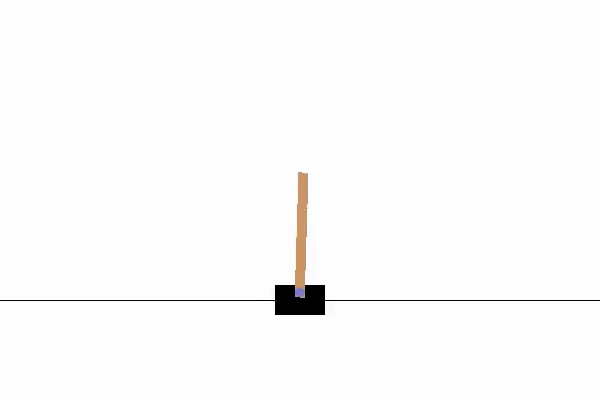
(a) CartPole

(b) Walker

(c) Hopper

(d) HalfCheetah

Figure 1: Four environments we used. (a) Cartpole: balance a pole on a cart; (b) Walker: make a 2D robot walk; (c) Hopper: make a 2D robot hop; (d) HalfCheetah: make a 2D cheetah robot run.

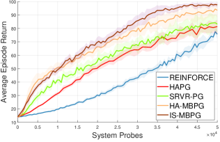
(a) CartPole

(b) Walker

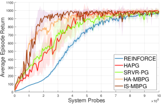
(c) Hopper

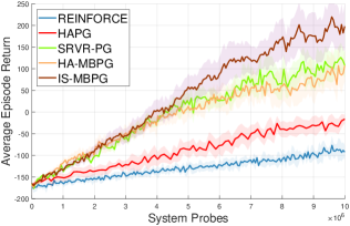
(d) HalfCheetah

Figure 2: Experimental results of our algorithms (IS-MBPG and HA-MBPG) and baseline algorithms at four environments.

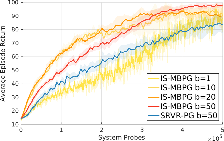
(a) IS-MBPG

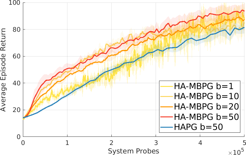
(b) HA-MBPG

Figure 3: Different batch sizes for our algorithms (IS-MBPG and HA-MBPG) at CartPole environment.

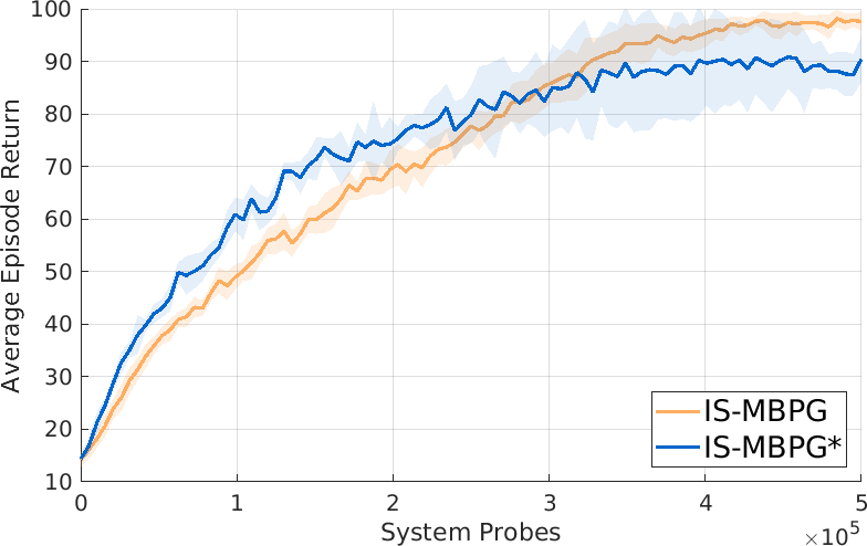
(a) CartPole

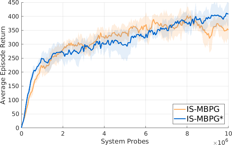
(b) Walker

Figure 4: Results of IS-MBPG and IS-MBPG* algorithms at CartPole and Walker environments.

5 Experiments

In this section, we demonstrate the performance of our algorithms on four standard reinforcement learning tasks, which are CartPole, Walker, HalfCheetah and Hopper. The first one is a discrete task from classic control, and the later three tasks are continuous RL task, which are popular MuJoCo environments (Todorov et al., 2012). Detailed description of these environments is shown in Fig. 1. Our code is publicly available on https://github.com/gaosh/MBPG.

5.1 Experimental Setup

In the experiment, we use Categorical Policy for CartPole, and Gaussian Policy for all the other environments. All Policies are parameterized by the fully connected neural network. The detail of network architecture and activation function used are shown in the Appendix A. The network settings are similar to the HAPG (Shen et al., 2019) algorithm. We implement our algorithms by using garage (garage contributors, 2019) and pytorch (Paszke et al., 2019). Note that Previous works mostly use environments implemented by old versions of garage, while latest version of garage directly use environments from gym (Brockman et al., 2016). As a result, there might be an inconsistency of the reward calculation between this paper and previous works due to the difference of environment implementation.

In the experiments, we compare our algorithm with the existing two best algorithms: Hessian Aided Policy Gradient (HAPG) (Shen et al., 2019), Stochastic Recursive Variance Reduced Policy Gradient (SRVR-PG) (Xu et al., 2019b) and a baseline algorithm: REINFORCE (Sutton et al., 2000). For a fair comparison, the policies of all methods use the same initialization, which ensures that they have similar start point. Moreover, to ease the impact of randomness, we run each method 10 times, and plot mean as well as variance interval for each of them.

In addition, for the purpose of fair comparison, we use the same batch size $\lvert\mathcal{B}\rvert$ for all algorithms, though our algorithms do not have a requirement on it. HAPG and SRVR-PG have sub-iterations (or inner loop), and requires additional hyper-parameters. The inner batch size for HAPG and SRVR-PG is also set to be the same value. For all the other hyper-parameters, we try to make them be analogous to the settings in their original paper. One may argue that our algorithms need three hyper-parameters $k$, $m$ and $c$ to control the evolution of learning rate while for other algorithms one hyper parameter is enough to control the learning rate. However, it should be noticed that our algorithms do not involve any sub-iterations unlike HAPG and SRVR-PG. Introducing sub-iterations itself naturally bring more hyper-parameters such as the number of sub-iteration and the inner batch size. From this perspective, the hyper-parameter complexity of our algorithms resembles HAPG and SRVR-PG. The more details of hyper-parameter selection are shown in Appendix A.

Similar to the HAPG algorithm, we use the system probes (i.e., the number of state transitions) as the measurement of sample complexity instead of number of trajectories. The reason of doing so is because each trajectory may have different length of states due to a failure flag returned from the environment (often happens at the beginning of training). Besides this reason, if using the number of trajectories as complexity measurement and the environment can return a failure flag, a faster algorithm may have a lot more system probes given the same number of trajectories. We also use average episode return as used in HAPG (Shen et al., 2019).

5.2 Experimental Results

The results of experiments are presented in Fig. 2. In the CartPole environment, our IS-MBPG and HA-MBPG algorithms have better performances than the other methods. In the Walker environment, our algorithms start to have more advantages. Specifically, the average return of IS-MBPG and HA-MBPG grows rapidly at the beginning of training. Moreover, our IS-MBPG algorithm achieves the best final performance with a obvious margin. HA-MBPG performs similar compared to SRVR-PG and HAPG, though it has an advantage at the beginning. In Hopper environment, our IS-MBPG and HA-MBPG algorithms are significantly faster compared to all other methods, while the final average reward are similar for different algorithms. In HalfCheetah environment, IS-MBPG, HA-MBPG and SRVR-PG performs similarly at the beginning. In the end of training, IS-MBPG can achieve the best performance. We note that HAPG performs poorly on this task, which is probably because of the normalized gradient and fixed learning rate in their algorithm. For all tasks, HA-MBPG are always inferior to the IS-MBPG. One possible reason for this observation is that we use the estimated Hessian vector product instead of the exact Hessian vector product in HA-MBPG algorithm, which brings additional estimation error to the algorithm.

In Fig. 3, we plot the average reward when changing batch size in CartPole environment. From Fig. 3, we find that when $20\%$ of the original batch size, our HA-MBPG and IS-MBPG algorithms still outperform the HAPG and SRVR-PG algorithms, respectively. When the batch size is 1, our HA-MBPG and IS-MBPG algorithms still reach a good performance. These results demonstrate that our HA-MBPG and IS-MBPG algorithms are not sensitive to the selection of batch size. Fig. 4 shows that the non-adaptive IS-MBPG* algorithm also has similar performances as the adaptive IS-MBPG algorithm.

6 Conclusion

In the paper, we proposed a class of efficient momentum-based policy gradient methods (i.e., IS-MBPG and HA-MBPG), which use adaptive learning rates and do not require any large batches. Moreover, we proved that both IS-MBPG and HA-MBPG methods reach the best known sample complexity of $O(\epsilon^{-3})$, which only require one trajectory at each iteration. In particular, we also presented a non-adaptive version of IS-MBPG method (i.e., IS-MBPG*), which has a simple monotonically decreasing learning rate. We proved that the IS-MBPG* also reaches the best known sample complexity of $O(\epsilon^{-3})$ only required one trajectory at each iteration.

Environments	CartPole	Walker	Hopper	HalfCheetah
Horizon	100	500	1000	500
Baseline	None	Linear	Linear	Linear
Neural Network (NN) sizes	$8\times 8$	$64\times 64$	$64\times 64$	$64\times 64$
NN activation function	Tanh	Tanh	Tanh	Tanh
Number of timesteps	$5\times 10^{5}$	$1\times 10^{7}$	$1\times 10^{7}$	$1\times 10^{7}$
Batch size $\lvert\mathcal{B}\rvert$	50	100	50	100
HAPG $\lvert\mathcal{B}_{\text{sub}}\rvert$	10	10	10	10
SRVR-PG $\lvert\mathcal{B}_{\text{sub}}\rvert$	10	10	10	10
HAPG $n_{\text{sub}}$	5	10	10	10
SRVR-PG $n_{\text{sub}}$	3	2	2	2
IS-MBPG/HA-MBPG $k$	0.75	0.75	0.75	0.75
IS-MBPG/HA-MBPG $c$	2	2	1	1
IS-MBPG/HA-MBPG $m$	2	12	3	3
IS-MBPG* $k$	0.9	0.9	-	-
IS-MBPG* $c$	2	2	-	-
IS-MBPG* $m$	2	12	-	-
REINFORCE learning rate $\eta$	0.01	0.01	0.01	0.01
HAPG learning rate $\eta$	0.01	0.01	0.01	0.01
SRVR-PG learning rate $\eta$	0.1	0.1	0.1	0.1

Table 2: Hyper-parameter Details. $\lvert\mathcal{B}_{\text{sub}}\rvert$ represents sub-iteration (inner-loop) batch size. $n_{\text{sub}}$ represents number of sub-iterations, which is called $p$ in the original paper of HAPG and $m$ in the oringinal paper of SRVR-PG. Although the learning rate $\eta$ of HAPG is given a small value $\eta=\epsilon$ in the theoretical analysis, we choose learning rate $\eta=0.01$ as given in the experiments of (Shen et al., 2019).

Appendix A Supplementary Materials for “Momentum-Based Policy Gradient Methods”

In this section, we first provide the details of hyper-parameter selection for the algorithms in Table 2. Table 2 also shows that the detail of network architecture and activation function used in the experiments. Next, we study the convergence properties of our algorithms. We begin with giving some useful lemmas.

Lemma 1.

(Lemma 1 in (Cortes et al., 2010)) Let $w(x)=P(x)/Q(x)$ be the importance weight for distributions $P$ and $Q$. The following identities hold for the expectation, second moment, and variance of $w(x)$

$$\mathbb{E}[w(x)]=1,\ \mathbb{E}[w^{2}(x)]=d_{2}(P||Q),\ \mathbb{V}[w(x)]=d_{2}(P||Q)-1,$$ (20)

where $d_{2}(P||Q)=2^{D(P||Q)}$, and $D(P||Q)$ is the $R\acute{e}nyi$ divergence between distributions $P$ and $Q$.

Lemma 2.

Under Assumptions 1 and 3, let $w(\tau|\theta_{t-1},\theta_{t})=g(\tau|\theta_{t-1})/g(\tau|\theta_{t})$, we have

$$\mathbb{V}[w(\tau|\theta_{t-1},\theta_{t})]\leq C^{2}_{w}\|\theta_{t}-\theta_{t-1}\|^{2},$$ (21)

where $C_{w}=\sqrt{H(2HM_{g}^{2}+M_{h})(W+1)}$.

Proof.

This proof can easy follow the proof of Lemma 6.1 in (Xu et al., 2019a). ∎

Lemma 3.

Under Assumption 1, let $e_{t}=\nabla J(\theta_{t})-u_{t}$. Given $0<\eta_{t}\leq\frac{1}{2L}$ for all $t\geq 1$, we have

$$\mathbb{E}[J(\theta_{t+1})]\geq\mathbb{E}[J(\theta_{t})-\frac{3\eta_{t}}{4}\|e_{t}\|^{2}+\frac{\eta_{t}}{8}\|\nabla J(\theta_{t})\|^{2}].$$ (22)

Proof.

Let $e_{t}=\nabla J(\theta_{t})-u_{t}$. By using $J(\theta)$ is $L$-smooth, we have

$$\mathbb{E}[J(\theta_{t+1})] \geq\mathbb{E}[J(\theta_{t})+\nabla J(\theta_{t})^{T}(\theta_{t+1}-\theta_{t})-\frac{L}{2}\|\theta_{t+1}-\theta_{t}\|^{2}]=\mathbb{E}[J(\theta_{t})+\eta_{t}\nabla J(\theta_{t})^{T}u_{t}-\frac{L\eta_{t}^{2}}{2}\|u_{t}\|^{2}]$$

$$=\mathbb{E}[J(\theta_{t})+\eta_{t}(\nabla J(\theta_{t})-u_{t})^{T}u_{t}+\eta_{t}\|u_{t}\|^{2}-\frac{L\eta_{t}^{2}}{2}\|u_{t}\|^{2}]$$

$$\geq\mathbb{E}[J(\theta_{t})-\frac{\eta_{t}}{2}\|\nabla J(\theta_{t})-u_{t}\|^{2}+\frac{\eta_{t}}{2}(1-L\eta_{t})\|u_{t}\|^{2}]$$

$$\geq\mathbb{E}[J(\theta_{t})-\frac{\eta_{t}}{2}\|\nabla J(\theta_{t})-u_{t}\|^{2}+\frac{\eta_{t}}{4}\|u_{t}\|^{2}]$$

$$\geq\mathbb{E}[J(\theta_{t})-\frac{3\eta_{t}}{4}\|e_{t}\|^{2}+\frac{\eta_{t}}{8}\|\nabla J(\theta_{t})\|^{2}],$$ (23)

where the second inequality holds by Young’s inequality, and the third inequality holds by $0<\eta_{t}\leq\frac{1}{2L}$, and the last inequality follows by $\|\nabla J(\theta_{t})\|^{2}\leq 2\|u_{t}\|^{2}+2\|\nabla J(\theta_{t})-u_{t}\|^{2}=2\|u_{t}\|^{2}+2\|e_{t}\|^{2}$. ∎

A.1 Convergence Analysis of IS-MBPG Algorithm

In this subsection, we analyze the convergence properties of IS-MBPG algorithm. For notational simplicity, let $\nabla J(\theta)$ denote $\nabla_{\theta}J(\theta)$.

Lemma 4.

Assume that the stochastic policy gradient $u_{t}$ be generated from Algorithm 1, and let $e_{t}=u_{t}-\nabla J(\theta_{t})$, we have

$$\mathbb{E}\big{[}\eta^{-1}_{t-1}\|e_{t}\|^{2}\big{]}\leq 2\beta^{2}_{t}\eta^{-1}_{t-1}G_{t}^{2}+\eta^{-1}_{t-1}(1-\beta_{t})^{2}\big{(}1+8\eta^{2}_{t-1}B^{2}\big{)}\mathbb{E}\|e_{t-1}\|^{2}+8(1-\beta_{t})^{2}B^{2}\eta_{t-1}\|\nabla J(\theta_{t-1})\|^{2},$$

where $B^{2}=L^{2}+2G^{2}C^{2}_{w}$ with $C_{w}=\sqrt{H(2HM_{g}^{2}+M_{h})(W+1)}$.

Proof.

By the definition of $u_{t}$ in Algorithm 1, we have

$$u_{t}-u_{t-1}=-\beta_{t}u_{t-1}+\beta_{t}g(\tau_{t}|\theta_{t})+(1-\beta_{t})\big{(}g(\tau_{t}|\theta_{t})-w(\tau_{t}|\theta_{t-1},\theta_{t})g(\tau_{t}|\theta_{t-1})\big{)}.$$ (24)

Then we have

$$\mathbb{E}\big{[}\eta^{-1}_{t-1}\|e_{t}\|^{2}\big{]} =\mathbb{E}\big{[}\eta^{-1}_{t-1}\|\nabla J(\theta_{t-1})-u_{t-1}+\nabla J(\theta_{t})-\nabla J(\theta_{t-1})-(u_{t}-u_{t-1})\|^{2}\big{]}$$ (25)

$$=\mathbb{E}\big{[}\eta^{-1}_{t-1}\|\nabla J(\theta_{t-1})-u_{t-1}+\nabla J(\theta_{t})-\nabla J(\theta_{t-1})+\beta_{t}u_{t-1}-\beta_{t}g(\tau_{t}|\theta_{t})$$

$$\quad-(1-\beta_{t})\big{(}g(\tau_{t}|\theta_{t})-w(\tau_{t}|\theta_{t-1},\theta_{t})g(\tau_{t}|\theta_{t-1})\big{)}\|^{2}\big{]}$$

$$=\mathbb{E}\big{[}\eta^{-1}_{t-1}\|(1-\beta_{t})(\nabla J(\theta_{t-1})-u_{t-1})+\beta_{t}(\nabla J(\theta_{t})-g(\tau_{t}|\theta_{t}))$$

$$\quad-(1-\beta_{t})\big{(}g(\tau_{t}|\theta_{t})-w(\tau_{t}|\theta_{t-1},\theta_{t})g(\tau_{t}|\theta_{t-1})-(\nabla J(\theta_{t})-\nabla J(\theta_{t-1}))\big{)}\|^{2}\big{]}$$

$$=\eta^{-1}_{t-1}(1-\beta_{t})^{2}\mathbb{E}\|\nabla J(\theta_{t-1})-u_{t-1}\|^{2}+\eta^{-1}_{t-1}\mathbb{E}\big{[}\|\beta_{t}(\nabla J(\theta_{t})-g(\tau_{t}|\theta_{t}))$$

$$\quad-(1-\beta_{t})\big{(}g(\tau_{t}|\theta_{t})-w(\tau_{t}|\theta_{t-1},\theta_{t})g(\tau_{t}|\theta_{t-1})-(\nabla J(\theta_{t})-\nabla J(\theta_{t-1}))\big{)}\|^{2}\big{]}$$

$$\leq\eta^{-1}_{t-1}(1-\beta_{t})^{2}\mathbb{E}\|\nabla J(\theta_{t-1})-u_{t-1}\|^{2}+2\beta^{2}_{t}\eta^{-1}_{t-1}\mathbb{E}\|\nabla J(\theta_{t})-g(\tau_{t}|\theta_{t})\|^{2}$$

$$\quad+2(1-\beta_{t})^{2}\mathbb{E}\|g(\tau_{t}|\theta_{t})-w(\tau_{t}|\theta_{t-1},\theta_{t})g(\tau_{t}|\theta_{t-1})-(\nabla J(\theta_{t})-\nabla J(\theta_{t-1}))\|^{2}$$

$$\leq\eta^{-1}_{t-1}(1-\beta_{t})^{2}\mathbb{E}\|e_{t-1}\|^{2}+2\beta^{2}_{t}\eta^{-1}_{t-1}\mathbb{E}\|g(\tau_{t}|\theta_{t})\|^{2}+2(1-\beta_{t})^{2}\eta^{-1}_{t-1}\mathbb{E}\|g(\tau_{t}|\theta_{t})-w(\tau_{t}|\theta_{t-1},\theta_{t})g(\tau_{t}|\theta_{t-1})\|^{2}$$

$$=\eta^{-1}_{t-1}(1-\beta_{t})^{2}\mathbb{E}\|e_{t-1}\|^{2}+2\beta^{2}_{t}\eta^{-1}_{t-1}G_{t}^{2}+2(1-\beta_{t})^{2}\eta^{-1}_{t-1}\underbrace{\mathbb{E}\|g(\tau_{t}|\theta_{t})-w(\tau_{t}|\theta_{t-1},\theta_{t})g(\tau_{t}|\theta_{t-1})\|^{2}}_{=T_{1}},$$

where the forth equality holds by $\mathbb{E}_{\tau_{t}\sim p(\tau|\theta_{t})}[g(\tau_{t}|\theta_{t})]=\nabla J(\theta_{t})$ and $\mathbb{E}_{\tau_{t}\sim p(\tau|\theta_{t})}[g(\tau_{t}|\theta_{t})-w(\tau_{t}|\theta_{t-1},\theta_{t})g(\tau_{t}|\theta_{t-1})]=\nabla J(\theta_{t})-\nabla J(\theta_{t-1})$; the first inequality follows by Young’s inequality; and the last inequality holds by $\mathbb{E}\|\zeta-\mathbb{E}[\zeta]\|^{2}=\mathbb{E}\|\zeta\|^{2}-(\mathbb{E}[\zeta])^{2}\leq\mathbb{E}\|\zeta\|^{2}$.

Next, we give an upper bound of the term $T_{1}$ as follows:

$$T_{1} =\mathbb{E}\|g(\tau_{t}|\theta_{t})-w(\tau_{t}|\theta_{t-1},\theta_{t})g(\tau_{t}|\theta_{t-1})\|^{2}$$

$$=\mathbb{E}\|g(\tau_{t}|\theta_{t})-g(\tau_{t}|\theta_{t-1})+g(\tau_{t}|\theta_{t-1})-w(\tau_{t}|\theta_{t-1},\theta_{t})g(\tau_{t}|\theta_{t-1})\|^{2}$$

$$\leq 2\mathbb{E}\|g(\tau_{t}|\theta_{t})-g(\tau_{t}|\theta_{t-1})\|^{2}+2\mathbb{E}\|(1-w(\tau_{t}|\theta_{t-1},\theta_{t}))g(\tau_{t}|\theta_{t-1})\|^{2}$$

$$\leq 2L^{2}\|\theta_{t}-\theta_{t-1}\|^{2}+2G^{2}\mathbb{E}\|1-w(\tau_{t}|\theta_{t-1},\theta_{t})\|^{2}$$

$$=2L^{2}\|\theta_{t}-\theta_{t-1}\|^{2}+2G^{2}\mathbb{V}\big{(}w(\tau_{t}|\theta_{t-1},\theta_{t})\big{)}$$

$$\leq 2(L^{2}+2G^{2}C^{2}_{w})\|\theta_{t}-\theta_{t-1}\|^{2},$$ (26)

where the second inequality holds by Proposition 1, and the third equality holds by Lemma 1, and the last inequality follows by Lemma 2.

Combining the inequalities (25) with (A.1), let $B^{2}=L^{2}+2G^{2}C^{2}_{w}$, we have

$$\mathbb{E}\big{[}\eta^{-1}_{t-1}\|e_{t}\|^{2}\big{]} \leq\eta^{-1}_{t-1}(1-\beta_{t})^{2}\mathbb{E}\|e_{t-1}\|^{2}+2\beta^{2}_{t}\eta^{-1}_{t-1}G_{t}^{2}+4(1-\beta_{t})^{2}\eta^{-1}_{t-1}B^{2}\|\theta_{t}-\theta_{t-1}\|^{2}$$

$$=\eta^{-1}_{t-1}(1-\beta_{t})^{2}\mathbb{E}\|e_{t-1}\|^{2}+2\beta^{2}_{t}\eta^{-1}_{t-1}G_{t}^{2}+4(1-\beta_{t})^{2}B^{2}\eta_{t-1}\|u_{t-1}\|^{2}$$

$$=\eta^{-1}_{t-1}(1-\beta_{t})^{2}\mathbb{E}\|e_{t-1}\|^{2}+2\beta^{2}_{t}\eta^{-1}_{t-1}G_{t}^{2}+4(1-\beta_{t})^{2}B^{2}\eta_{t-1}\|e_{t-1}+\nabla J(\theta_{t-1})\|^{2}$$

$$\leq 2\beta^{2}_{t}\eta^{-1}_{t-1}G_{t}^{2}+\eta^{-1}_{t-1}(1-\beta_{t})^{2}\big{(}1+8\eta^{2}_{t-1}B^{2}\big{)}\mathbb{E}\|e_{t-1}\|^{2}+8(1-\beta_{t})^{2}B^{2}\eta_{t-1}\|\nabla J(\theta_{t-1})\|^{2}.$$ (27)

∎

Theorem 4.

Assume that the sequence $\{\theta_{t}\}_{t=1}^{T}$ be generated from Algorithm 1, and let $B^{2}=L^{2}+2G^{2}C^{2}_{w}$, $k=O(\frac{G^{2/3}}{L})$ $c=\frac{G^{2}}{3k^{3}L}+104B^{2}$, $m=\max\{2G^{2},(2Lk)^{3},(\frac{ck}{2L})^{3}\}$ and $\eta_{0}=\frac{k}{m^{1/3}}$, we have

$$\mathbb{E}\|\nabla J(\theta_{\zeta})\|=\frac{1}{T}\sum_{t=1}^{T}\mathbb{E}\|\nabla J(\theta_{t})\|\leq\frac{\sqrt{2\Omega}m^{1/6}+2\Omega^{3/4}}{\sqrt{T}}+\frac{2\sqrt{\Omega}\sigma^{1/3}}{T^{1/3}},$$

where $\Omega=\frac{1}{k}\big{(}16(J^{*}-J(\theta_{1}))+\frac{m^{1/3}}{8B^{2}k}\sigma^{2}+\frac{c^{2}k^{3}}{4B^{2}}\ln(T+2)\big{)}$ with $J^{*}=\sup_{\theta}J(\theta)<+\infty$.

Proof.

Due to $m\geq(2Lk)^{3}$, we have $\eta_{t}\leq\frac{k}{m^{1/3}}\leq\frac{1}{2L}$. Since $\eta_{t}\leq\frac{1}{2L}$ and $m\geq(\frac{ck}{2L})^{3}$, we have $\beta_{t+1}=c\eta^{2}_{t}\leq\frac{c\eta_{t}}{2L}\leq\frac{ck}{2Lm^{1/3}}\leq 1$. By Lemma 4, we have

$$\mathbb{E}[\eta^{-1}_{t}\|e_{t+1}\|^{2}-\eta^{-1}_{t-1}\|e_{t}\|^{2}] \leq\mathbb{E}\big{[}2\beta^{2}_{t+1}\eta^{-1}_{t}G_{t+1}^{2}+\eta^{-1}_{t}(1-\beta_{t+1})^{2}\big{(}1+8\eta^{2}_{t}B^{2}\big{)}\|e_{t}\|^{2}$$

$$\quad+8(1-\beta_{t+1})^{2}B^{2}\eta_{t}\|\nabla J(\theta_{t})\|^{2}-\eta^{-1}_{t-1}\|e_{t}\|^{2}\big{]}$$

$$\leq\mathbb{E}\big{[}2c^{2}\eta^{3}_{t}G_{t+1}^{2}+\underbrace{\big{(}\eta^{-1}_{t}(1-\beta_{t+1})(1+8\eta^{2}_{t}B^{2})-\eta^{-1}_{t-1}\big{)}\|e_{t}\|^{2}}_{=T_{2}}+8B^{2}\eta_{t}\|\nabla J(\theta_{t})\|^{2}\big{]},$$ (28)

where the last inequality holds by $0<\beta_{t+1}\leq 1$. Since the function $x^{1/3}$ is cancave, we have $(x+y)^{1/3}\leq x^{1/3}+yx^{-2/3}/3$. Then we have

$$\eta^{-1}_{t}-\eta^{-1}_{t-1} =\frac{1}{k}\bigg{(}\big{(}m+\sum_{i=1}^{t}G^{2}_{i}\big{)}^{1/3}-\big{(}m+\sum_{i=1}^{t-1}G^{2}_{i}\big{)}^{1/3}\bigg{)}\leq\frac{G^{2}_{t}}{3k(m+\sum_{i=1}^{t-1}G^{2}_{i})^{2/3}}$$

$$\leq\frac{G^{2}_{t}}{3k(m-G^{2}+\sum_{i=1}^{t}G^{2}_{i})^{2/3}}\leq\frac{G^{2}_{t}}{3k(m/2+\sum_{i=1}^{t}G^{2}_{i})^{2/3}}\leq\frac{2^{2/3}G^{2}_{t}}{3k(m+\sum_{i=1}^{t}G^{2}_{i})^{2/3}}$$

$$\leq\frac{2^{2/3}G^{2}}{3k^{3}}\eta_{t}^{2}\leq\frac{2^{2/3}G^{2}}{6k^{3}L}\eta_{t}\leq\frac{G^{2}}{3k^{3}L}\eta_{t},$$ (29)

where the third inequality holds by $m\geq 2G^{2}$, and the sixth inequality holds by $0<\eta\leq\frac{1}{2L}$.

Next, considering the upper bound of the term $T_{2}$, we have

$$T_{2} =\big{(}\eta^{-1}_{t}(1-\beta_{t+1})(1+8\eta^{2}_{t}B^{2})-\eta^{-1}_{t-1}\big{)}\|e_{t}\|^{2}$$

$$=\big{(}\eta^{-1}_{t}-\eta^{-1}_{t-1}+8B^{2}\eta_{t}-\beta_{t+1}\eta^{-1}_{t}-8\eta_{t}\beta_{t+1}B^{2}\big{)}\|e_{t}\|^{2}$$

$$\leq\big{(}\eta^{-1}_{t}-\eta^{-1}_{t-1}+8B^{2}\eta_{t}-\beta_{t+1}\eta^{-1}_{t}\big{)}\|e_{t}\|^{2}$$

$$\leq\big{(}\frac{G^{2}}{3k^{3}L}\eta_{t}+8B^{2}\eta_{t}-c\eta_{t}\big{)}\|e_{t}\|^{2}=-96B^{2}\eta_{t}\|e_{t}\|^{2},$$ (30)

where the last equality holds by $c=\frac{G^{2}}{3k^{3}L}+104B^{2}$. Combining the inequalities (A.1) with (A.1), we have

$$\mathbb{E}[\eta^{-1}_{t}\|e_{t+1}\|^{2}-\eta^{-1}_{t-1}\|e_{t}\|^{2}]\leq\mathbb{E}\big{[}2c^{2}\eta^{3}_{t}G_{t+1}^{2}-96B^{2}\eta_{t}\|e_{t}\|^{2}+8B^{2}\eta_{t}\|\nabla J(\theta_{t})\|^{2}\big{]}.$$ (31)

We define a Lyapunov function $\Phi_{t}=J(\theta_{t})-\frac{1}{128B^{2}\eta_{t-1}}\|e_{t}\|^{2}$ for any $t\geq 1$. Then we have

$$\mathbb{E}[\Phi_{t+1}-\Phi_{t}] =\mathbb{E}\big{[}J(\theta_{t+1})-J(\theta_{t})-\frac{1}{128B^{2}\eta_{t}}\|e_{t+1}\|^{2}+\frac{1}{128B^{2}\eta_{t-1}}\|e_{t}\|^{2}\big{]}$$

$$\geq\mathbb{E}\big{[}-\frac{3\eta_{t}}{4}\|e_{t}\|^{2}+\frac{\eta_{t}}{8}\|\nabla J(\theta_{t})\|^{2}-\frac{1}{128B^{2}}(\eta^{-1}_{t}\|e_{t+1}\|^{2}-\eta^{-1}_{t-1}\|e_{t}\|^{2})\big{]}$$

$$\geq-\frac{c^{2}\eta^{3}_{t}G_{t+1}^{2}}{64B^{2}}+\frac{\eta_{t}}{16}\mathbb{E}\|\nabla J(\theta_{t})\|^{2},$$ (32)

where the first inequality holds by the Lemma 3, and the second inequality follows by the above inequality (31). Summing the above inequality (A.1) over $t$ from $1$ to $T$, we obtain

$$\sum_{t=1}^{T}\mathbb{E}[\eta_{t}\|\nabla J(\theta_{t})\|^{2}] \leq\mathbb{E}[16(\Phi_{T+1}-\Phi_{1})]+\sum_{t=1}^{T}\frac{c^{2}\eta^{3}_{t}G_{t+1}^{2}}{4B^{2}}$$

$$\leq\mathbb{E}[16(J^{*}-J(\theta_{1}))]+\frac{1}{8B^{2}\eta_{0}}\mathbb{E}\|e_{1}\|^{2}+\frac{c^{2}k^{3}}{4B^{2}}\sum_{t=1}^{T}\frac{G_{t+1}^{2}}{m+\sum_{i=1}^{t}G_{i}^{2}}$$

$$\leq\mathbb{E}[16(J^{*}-J(\theta_{1}))]+\frac{1}{8B^{2}\eta_{0}}\mathbb{E}\|e_{1}\|^{2}+\frac{c^{2}k^{3}}{4B^{2}}\sum_{t=1}^{T}\frac{G_{t+1}^{2}}{G^{2}+\sum_{i=1}^{t+1}G_{i}^{2}}$$

$$\leq\mathbb{E}[16(J^{*}-J(\theta_{1}))]+\frac{1}{8B^{2}\eta_{0}}\mathbb{E}\|e_{1}\|^{2}+\frac{c^{2}k^{3}}{4B^{2}}\sum_{t=1}^{T}\big{(}\ln(G^{2}+\sum_{i=1}^{t+1}G_{i}^{2})-\ln(G^{2}+\sum_{i=1}^{t}G_{i}^{2})\big{)}$$

$$\leq\mathbb{E}[16(J^{*}-J(\theta_{1}))]+\frac{1}{8B^{2}\eta_{0}}\mathbb{E}\|e_{1}\|^{2}+\frac{c^{2}k^{3}}{4B^{2}}(\ln(G^{2}+\sum_{i=1}^{T+1}G_{i}^{2})-\ln(G^{2}))$$

$$\leq\mathbb{E}[16(J^{*}-J(\theta_{1}))]+\frac{m^{1/3}}{8B^{2}k}\sigma^{2}+\frac{c^{2}k^{3}}{4B^{2}}\ln(1+\sum_{i=1}^{T+1}\frac{G_{i}^{2}}{G^{2}})$$

$$\leq\mathbb{E}[16(J^{*}-J(\theta_{1}))]+\frac{m^{1/3}}{8B^{2}k}\sigma^{2}+\frac{c^{2}k^{3}}{4B^{2}}\ln(T+2),$$ (33)

where $J^{*}=\sup_{\theta}J(\theta)<+\infty$, and the fourth inequality holds by the concavity of the function $\ln(x)$, and the sixth inequality holds by the definition of $e_{1}$ and $\eta_{0}$.

By Cauchy-Schwarz inequality, we have $\mathbb{E}[XY]^{2}\leq\mathbb{E}[X^{2}]\mathbb{E}[Y^{2}]$. Let $X=\sqrt{\eta_{T}\sum_{t=1}^{T-1}\|\nabla J(\theta_{t})\|^{2}}$ and $Y=\sqrt{1/\eta_{T}}$, we have

$$\mathbb{E}\big{[}\sum_{t=1}^{T}\|\nabla J(\theta_{t})\|^{2}\big{]}\leq\mathbb{E}[1/\eta_{T}]\mathbb{E}\big{[}\eta_{T}\sum_{t=1}^{T}\|\nabla J(\theta_{t})\|^{2}\big{]}.$$ (34)

Since $\eta_{t}$ is decreasing, we have

$$\mathbb{E}\big{[}\sum_{t=1}^{T}\|\nabla J(\theta_{t})\|^{2}\big{]}\leq\mathbb{E}[1/\eta_{T}]\mathbb{E}\big{[}\sum_{t=1}^{T}\eta_{T}\|\nabla J(\theta_{t})\|^{2}\big{]}\leq\mathbb{E}[1/\eta_{T}]\mathbb{E}\big{[}\sum_{t=1}^{T}\eta_{t}\|\nabla J(\theta_{t})\|^{2}\big{]}.$$ (35)

Combining the inequalities (A.1) and (35), we obtain

$$\mathbb{E}\big{[}\sum_{t=1}^{T}\|\nabla J(\theta_{t})\|^{2}\big{]} \leq\mathbb{E}\big{[}\frac{16(J^{*}-J(\theta_{1}))+\frac{m^{1/3}}{8B^{2}k}\sigma^{2}+\frac{c^{2}k^{3}}{4B^{2}}\ln(T+2)}{\eta_{T}}\big{]}$$

$$=\mathbb{E}\big{[}\Omega\big{(}m+\sum_{t=1}^{T}G^{2}_{t}\big{)}^{1/3}\big{]}$$ (36)

where $\Omega=\frac{1}{k}\big{(}16(J^{*}-J(\theta_{1}))+\frac{m^{1/3}}{8B^{2}k}\sigma^{2}+\frac{c^{2}k^{3}}{4B^{2}}\ln(T+2)\big{)}$.

By Assumption 2, we have $G^{2}_{t}=\|g(\tau|\theta_{t})-\nabla J(\theta_{t})+\nabla J(\theta_{t})\|^{2}\leq 2\|g(\tau|\theta_{t})-\nabla J(\theta_{t})\|^{2}+2\|\nabla J(\theta_{t})\|^{2}\leq 2\sigma^{2}+2\|\nabla J(\theta_{t})\|^{2}$. Then using the inequality $(a+b)^{1/3}\leq a^{1/3}+b^{1/3}$ for all $a,b>0$ to the inequality (A.1), we obtain

$$\bigg{(}\mathbb{E}\sqrt{\sum_{t=1}^{T}\|\nabla J(\theta_{t})\|^{2}}\bigg{)}^{2} \leq\mathbb{E}\bigg{[}\sqrt{\sum_{t=1}^{T}\|\nabla J(\theta_{t})\|^{2}}\bigg{]}^{2}=\mathbb{E}\big{[}\sum_{t=1}^{T}\|\nabla J(\theta_{t})\|^{2}\big{]}$$

$$\leq\mathbb{E}\bigg{[}\Omega(m+2T\sigma^{2})^{1/3}+2^{1/3}\Omega\big{(}\sum_{t=1}^{T}\|\nabla J(\theta_{t})\|^{2}\big{)}^{1/3}\bigg{]}$$

$$=\Omega(m+2T\sigma^{2})^{1/3}+2^{1/3}\Omega\mathbb{E}\bigg{[}\sqrt{\sum_{t=1}^{T}\|\nabla J(\theta_{t})\|^{2}}\bigg{]}^{2/3}$$

$$\leq\Omega(m+2T\sigma^{2})^{1/3}+2^{1/3}\Omega\bigg{[}\mathbb{E}\sqrt{\sum_{t=1}^{T}\|\nabla J(\theta_{t})\|^{2}}\bigg{]}^{2/3},$$ (37)

where the first inequality holds by the convexity of the function $x^{2}$, and the last inequality holds by the concavity of the function $x^{2/3}$. For simplicity, let $Z=\sqrt{\sum_{t=1}^{T}\|\nabla J(\theta_{t})\|^{2}}$, we have

$$\big{(}\mathbb{E}[Z]\big{)}^{2}\leq\Omega(m+2T\sigma^{2})^{1/3}+2^{1/3}\Omega\big{(}\mathbb{E}[Z]\big{)}^{2/3}.$$ (38)

The inequality (38) implies that $\big{(}\mathbb{E}[Z]\big{)}^{2}\leq 2\Omega(m+2T\sigma^{2})^{1/3}$ or $\big{(}\mathbb{E}[Z]\big{)}^{2}\leq 2\cdot 2^{1/3}\Omega\big{(}\mathbb{E}[Z]\big{)}^{2/3}$. Thus, we have

$$\mathbb{E}[Z]\leq\sqrt{2\Omega}(m+2T\sigma^{2})^{1/6}+2\Omega^{3/4}.$$ (39)

By Cauchy-Schwarz inequality, then we have

$$\frac{1}{T}\sum_{t=1}^{T}\mathbb{E}\|\nabla J(\theta_{t})\| =\mathbb{E}\big{[}\frac{1}{T}\sum_{t=1}^{T}\|\nabla J(\theta_{t})\|\big{]}\leq\mathbb{E}\bigg{[}\sqrt{\frac{1}{T}}\sqrt{\sum_{t=1}^{T}\|\nabla J(\theta_{t})\|^{2}}\bigg{]}$$

$$\leq\frac{\sqrt{2\Omega}(m+2T\sigma^{2})^{1/6}+2\Omega^{3/4}}{\sqrt{T}}$$

$$\leq\frac{\sqrt{2\Omega}m^{1/6}+2\Omega^{3/4}}{\sqrt{T}}+\frac{2\sqrt{\Omega}\sigma^{1/3}}{T^{1/3}},$$ (40)

where the last inequality follows by the inequality $(a+b)^{1/6}\leq a^{1/6}+b^{1/6}$ for all $a,b>0$. ∎

A.2 Convergence Analysis of HA-MBPG Algorithm

In this subsection, we analyze the convergence properties of HA-MBPG algorithm.

Lemma 5.

Assume that the stochastic policy gradient $u_{t}$ be generated from Algorithm 2. Let $e_{t}=u_{t}-\nabla J(\theta_{t})$, we have

$$\mathbb{E}\big{[}\eta^{-1}_{t-1}\|e_{t}\|^{2}\big{]}\leq 4(W+1)\beta^{2}_{t}\eta^{-1}_{t-1}G_{t}^{2}+\eta^{-1}_{t-1}(1-\beta_{t})^{2}\big{(}1+4\eta^{2}_{t-1}L^{2}\big{)}\mathbb{E}\|e_{t-1}\|^{2}+4(1-\beta_{t})^{2}L^{2}\eta_{t-1}\|\nabla J(\theta_{t-1})\|^{2}.$$

Proof.

By the definition of $u_{t}$ in Algorithm 2, we have

$$u_{t}-u_{t-1}=-\beta_{t}u_{t-1}+\beta_{t}w(\tau_{t}|\theta_{t},\theta_{t}(\alpha))g(\tau_{t}|\theta_{t})+(1-\beta_{t})\Delta_{t}.$$ (41)

Then we have

$$\mathbb{E}\big{[}\eta^{-1}_{t-1}\|e_{t}\|^{2}\big{]} =\mathbb{E}\big{[}\eta^{-1}_{t-1}\|\nabla J(\theta_{t-1})-u_{t-1}+\nabla J(\theta_{t})-\nabla J(\theta_{t-1})-(u_{t}-u_{t-1})\|^{2}\big{]}$$ (42)

$$=\mathbb{E}\big{[}\eta^{-1}_{t-1}\|\nabla J(\theta_{t-1})-u_{t-1}+\nabla J(\theta_{t})-\nabla J(\theta_{t-1})+\beta_{t}u_{t-1}-\beta_{t}w(\tau_{t}|\theta_{t},\theta_{t}(\alpha))g(\tau_{t}|\theta_{t})-(1-\beta_{t})\Delta_{t}\big{]}$$

$$=\mathbb{E}\big{[}\eta^{-1}_{t-1}\|(1-\beta_{t})(\nabla J(\theta_{t-1})-u_{t-1})+\beta_{t}(\nabla J(\theta_{t})-w(\tau_{t}|\theta_{t},\theta_{t}(\alpha))g(\tau_{t}|\theta_{t}))$$

$$\quad-(1-\beta_{t})\big{(}\Delta_{t}-(\nabla J(\theta_{t})-\nabla J(\theta_{t-1}))\big{)}\|^{2}\big{]}$$

$$=\eta^{-1}_{t-1}(1-\beta_{t})^{2}\mathbb{E}\|\nabla J(\theta_{t-1})-u_{t-1}\|^{2}+\eta^{-1}_{t-1}\mathbb{E}\big{[}\|\beta_{t}(\nabla J(\theta_{t})-w(\tau_{t}|\theta_{t},\theta_{t}(\alpha))g(\tau_{t}|\theta_{t}))$$

$$\quad-(1-\beta_{t})\big{(}\Delta_{t}-(\nabla J(\theta_{t})-\nabla J(\theta_{t-1}))\big{)}\|^{2}\big{]}$$

$$\leq\eta^{-1}_{t-1}(1-\beta_{t})^{2}\mathbb{E}\|\nabla J(\theta_{t-1})-u_{t-1}\|^{2}+2\beta^{2}_{t}\eta^{-1}_{t-1}\mathbb{E}\|\nabla J(\theta_{t})-w(\tau_{t}|\theta_{t},\theta_{t}(\alpha))g(\tau_{t}|\theta_{t})\|^{2}$$

$$\quad+2(1-\beta_{t})^{2}\mathbb{E}\|\Delta_{t}-(\nabla J(\theta_{t})-\nabla J(\theta_{t-1}))\|^{2}$$

$$\leq\eta^{-1}_{t-1}(1-\beta_{t})^{2}\mathbb{E}\|e_{t-1}\|^{2}+2\beta^{2}_{t}\eta^{-1}_{t-1}\underbrace{\mathbb{E}\|w(\tau_{t}|\theta_{t},\theta_{t}(\alpha))g(\tau_{t}|\theta_{t})\|^{2}}_{=T_{3}}+2(1-\beta_{t})^{2}\eta^{-1}_{t-1}\mathbb{E}\|\Delta_{t}\|^{2},$$

where the forth equality holds by $\mathbb{E}_{\tau_{t}\sim p(\tau|\theta_{t}(\alpha))}[w(\tau_{t}|\theta_{t},\theta_{t}(\alpha))g(\tau_{t}|\theta_{t})]=\nabla J(\theta_{t})$ and $\mathbb{E}_{\tau_{t}\sim p(\tau|\theta_{t}(\alpha))}[\Delta_{t}]=\nabla J(\theta_{t})-\nabla J(\theta_{t-1})$; the first inequality follows by Young’s inequality; and the last inequality holds by $\mathbb{E}\|\zeta-\mathbb{E}[\zeta]\|^{2}=\mathbb{E}\|\zeta\|^{2}-(\mathbb{E}[\zeta])^{2}\leq\mathbb{E}\|\zeta\|^{2}$.

Next, we give an upper bound of the term $T_{3}$ as follows:

$$T_{3} =\mathbb{E}\|w(\tau_{t}|\theta_{t},\theta_{t}(\alpha))g(\tau_{t}|\theta_{t})\|^{2}$$

$$=\mathbb{E}\|w(\tau_{t}|\theta_{t},\theta_{t}(\alpha))g(\tau_{t}|\theta_{t})-g(\tau_{t}|\theta_{t})+g(\tau_{t}|\theta_{t})\|^{2}$$

$$\leq 2\mathbb{E}\|\big{(}w(\tau_{t}|\theta_{t},\theta_{t}(\alpha))-1\big{)}g(\tau_{t}|\theta_{t})\|^{2}+2\mathbb{E}\|g(\tau_{t}|\theta_{t})\|^{2}$$

$$\leq 2\mathbb{E}\|w(\tau_{t}|\theta_{t},\theta_{t}(\alpha))-1\|^{2}\mathbb{E}\|g(\tau_{t}|\theta_{t})\|^{2}+2\mathbb{E}\|g(\tau_{t}|\theta_{t})\|^{2}$$

$$\leq 2(W+1)G_{t}^{2},$$ (43)

where the last inequality holds by Proposition 1 and Assumption 3.

Finally, combining the inequalities (42) with (A.2), we have

$$\mathbb{E}\big{[}\eta^{-1}_{t-1}\|e_{t}\|^{2}\big{]} \leq\eta^{-1}_{t-1}(1-\beta_{t})^{2}\mathbb{E}\|e_{t-1}\|^{2}+4\beta^{2}_{t}\eta^{-1}_{t-1}(W+1)G_{t}^{2}+2(1-\beta_{t})^{2}\eta^{-1}_{t-1}\mathbb{E}\|\hat{\nabla}^{2}(\theta_{t},\tau)v\|^{2}$$

$$\leq\eta^{-1}_{t-1}(1-\beta_{t})^{2}\mathbb{E}\|e_{t-1}\|^{2}+4\beta^{2}_{t}\eta^{-1}_{t-1}(W+1)G_{t}^{2}+2(1-\beta_{t})^{2}\eta^{-1}_{t-1}L^{2}\mathbb{E}\|\theta_{t}-\theta_{t-1}\|^{2}$$

$$=\eta^{-1}_{t-1}(1-\beta_{t})^{2}\mathbb{E}\|e_{t-1}\|^{2}+4\beta^{2}_{t}\eta^{-1}_{t-1}(W+1)G_{t}^{2}+2(1-\beta_{t})^{2}L^{2}\eta_{t-1}\|e_{t-1}+\nabla J(\theta_{t-1})\|^{2}$$

$$\leq 4(W+1)\beta^{2}_{t}\eta^{-1}_{t-1}G_{t}^{2}+\eta^{-1}_{t-1}(1-\beta_{t})^{2}\big{(}1+4\eta^{2}_{t-1}L^{2}\big{)}\mathbb{E}\|e_{t-1}\|^{2}+4(1-\beta_{t})^{2}L^{2}\eta_{t-1}\|\nabla J(\theta_{t-1})\|^{2},$$

where the second inequality holds by the Proposition 2.

∎

Theorem 5.

Assume that the sequence $\{\theta_{t}\}_{t=1}^{T}$ be generated from Algorithm 2, and let $k=O(\frac{G^{2/3}}{L})$ $c=\frac{G^{2}}{3k^{3}L}+52L^{2}$, $m=\max\{2G^{2},(2Lk)^{3},(\frac{ck}{2L})^{3}\}$ and $\eta_{0}=\frac{k}{m^{1/3}}$, we have

$$\mathbb{E}\|\nabla J(\theta_{\zeta})\|=\frac{1}{T}\sum_{t=1}^{T}\mathbb{E}\|\nabla J(\theta_{t})\|\leq\frac{\sqrt{2\Lambda}m^{1/6}+2\Lambda^{3/4}}{\sqrt{T}}+\frac{2\sqrt{\Lambda}\sigma^{1/3}}{T^{1/3}},$$

where $\Lambda=\frac{1}{k}\big{(}16(J^{*}-J(\theta_{1}))+\frac{m^{1/3}}{4L^{2}k}\sigma^{2}+\frac{(W+1)c^{2}k^{3}}{2L^{2}}\ln(T+2)\big{)}$ with $J^{*}=\sup_{\theta}J(\theta)<+\infty$.

Proof.

This proof mainly follows the proof of the above Theorem 4. Due to $m\geq(2Lk)^{3}$, we have $\eta_{t}\leq\frac{k}{m^{1/3}}\leq\frac{1}{2L}$. Since $\eta_{t}\leq\frac{1}{2L}$ and $m\geq(\frac{ck}{2L})^{3}$, we have $\beta_{t+1}=c\eta^{2}_{t}\leq\frac{c\eta_{t}}{2L}\leq\frac{ck}{2Lm^{1/3}}\leq 1$. By Lemma 5, we have

$$\mathbb{E}[\eta^{-1}_{t}\|e_{t+1}\|^{2}-\eta^{-1}_{t-1}\|e_{t}\|^{2}] \leq\mathbb{E}\big{[}4(W+1)\beta^{2}_{t+1}\eta^{-1}_{t}G_{t+1}^{2}+\eta^{-1}_{t}(1-\beta_{t+1})^{2}\big{(}1+4\eta^{2}_{t}L^{2}\big{)}\|e_{t}\|^{2}$$

$$\quad+4(1-\beta_{t+1})^{2}L^{2}\eta_{t}\|\nabla J(\theta_{t})\|^{2}-\eta^{-1}_{t-1}\|e_{t}\|^{2}\big{]}$$

$$\leq\mathbb{E}\big{[}4(W+1)c^{2}\eta^{3}_{t}G_{t+1}^{2}+\underbrace{\big{(}\eta^{-1}_{t}(1-\beta_{t+1})(1+4\eta^{2}_{t}L^{2})-\eta^{-1}_{t-1}\big{)}\|e_{t}\|^{2}}_{=T_{4}}+4L^{2}\eta_{t}\|\nabla J(\theta_{t})\|^{2}\big{]},$$ (44)

where the last inequality holds by $0<\beta_{t+1}\leq 1$. Since the function $x^{1/3}$ is cancave, we have $(x+y)^{1/3}\leq x^{1/3}+yx^{-2/3}/3$. Then we have

$$\eta^{-1}_{t}-\eta^{-1}_{t-1} =\frac{1}{k}\bigg{(}\big{(}m+\sum_{i=1}^{t}G^{2}_{i}\big{)}^{1/3}-\big{(}m+\sum_{i=1}^{t-1}G^{2}_{i}\big{)}^{1/3}\bigg{)}\leq\frac{G^{2}_{t}}{3k(m+\sum_{i=1}^{t-1}G^{2}_{i})^{2/3}}$$

$$\leq\frac{G^{2}_{t}}{3k(m-G^{2}+\sum_{i=1}^{t}G^{2}_{i})^{2/3}}\leq\frac{G^{2}_{t}}{3k(m/2+\sum_{i=1}^{t}G^{2}_{i})^{2/3}}\leq\frac{2^{2/3}G^{2}_{t}}{3k(m+\sum_{i=1}^{t}G^{2}_{i})^{2/3}}$$

$$\leq\frac{2^{2/3}G^{2}}{3k^{3}}\eta_{t}^{2}\leq\frac{2^{2/3}G^{2}}{6k^{3}L}\eta_{t}\leq\frac{G^{2}}{3k^{3}L}\eta_{t},$$ (45)

where the third inequality holds by $m\geq 2G^{2}$, and the sixth inequality holds by $0<\eta\leq\frac{1}{2L}$.

Next, considering the upper bound of the term $T_{4}$, we have

$$T_{4} =\big{(}\eta^{-1}_{t}(1-\beta_{t+1})(1+4\eta^{2}_{t}L^{2})-\eta^{-1}_{t-1}\big{)}\|e_{t}\|^{2}$$

$$=\big{(}\eta^{-1}_{t}-\eta^{-1}_{t-1}+4L^{2}\eta_{t}-\beta_{t+1}\eta^{-1}_{t}-4\eta_{t}\beta_{t+1}L^{2}\big{)}\|e_{t}\|^{2}$$

$$\leq\big{(}\eta^{-1}_{t}-\eta^{-1}_{t-1}+4L^{2}\eta_{t}-\beta_{t+1}\eta^{-1}_{t}\big{)}\|e_{t}\|^{2}$$

$$\leq\big{(}\frac{G^{2}}{3k^{3}L}\eta_{t}+4L^{2}\eta_{t}-c\eta_{t}\big{)}\|e_{t}\|^{2}=-48L^{2}\eta_{t}\|e_{t}\|^{2},$$ (46)

where the last equality holds by $c=\frac{G^{2}}{3k^{3}L}+52L^{2}$. Combining the inequalities (A.2) with (A.2), we have

$$\mathbb{E}[\eta^{-1}_{t}\|e_{t+1}\|^{2}-\eta^{-1}_{t-1}\|e_{t}\|^{2}]\leq\mathbb{E}\big{[}4(W+1)c^{2}\eta^{3}_{t}G_{t+1}^{2}-48L^{2}\eta_{t}\|e_{t}\|^{2}+4L^{2}\eta_{t}\|\nabla J(\theta_{t})\|^{2}\big{]}.$$ (47)

We define a Lyapunov function $\Psi_{t}=J(\theta_{t})-\frac{1}{64L^{2}\eta_{t-1}}\|e_{t}\|^{2}$ for any $t\geq 1$. Then we have

$$\mathbb{E}[\Psi_{t+1}-\Psi_{t}] =\mathbb{E}\big{[}J(\theta_{t+1})-J(\theta_{t})-\frac{1}{64L^{2}\eta_{t}}\|e_{t+1}\|^{2}+\frac{1}{64L^{2}\eta_{t-1}}\|e_{t}\|^{2}\big{]}$$

$$\geq\mathbb{E}\big{[}-\frac{3\eta_{t}}{4}\|e_{t}\|^{2}+\frac{\eta_{t}}{8}\|\nabla J(\theta_{t})\|^{2}-\frac{1}{64L^{2}}(\eta^{-1}_{t}\|e_{t+1}\|^{2}-\eta^{-1}_{t-1}\|e_{t}\|^{2})\big{]}$$

$$\geq-\frac{(W+1)c^{2}\eta^{3}_{t}G_{t+1}^{2}}{32L^{2}}+\frac{\eta_{t}}{16}\mathbb{E}\|\nabla J(\theta_{t})\|^{2},$$ (48)

where the first inequality holds by the Lemma 3, and the second inequality follows by the above inequality (47). Summing the above inequality (A.2) over $t$ from $1$ to $T$, we obtain

$$\sum_{t=1}^{T}\mathbb{E}[\eta_{t}\|\nabla J(\theta_{t})\|^{2}] \leq\mathbb{E}[16(\Psi_{T+1}-\Psi_{1})]+\sum_{t=1}^{T}\frac{(W+1)c^{2}\eta^{3}_{t}G_{t+1}^{2}}{2L^{2}}$$

$$\leq\mathbb{E}[16(J^{*}-J(\theta_{1}))]+\frac{1}{4L^{2}\eta_{0}}\mathbb{E}\|e_{1}\|^{2}+\frac{(W+1)c^{2}k^{3}}{2L^{2}}\sum_{t=1}^{T}\frac{G_{t+1}^{2}}{m+\sum_{i=1}^{t}G_{i}^{2}}$$

$$\leq\mathbb{E}[16(J^{*}-J(\theta_{1}))]+\frac{1}{4L^{2}\eta_{0}}\mathbb{E}\|e_{1}\|^{2}+\frac{(W+1)c^{2}k^{3}}{2L^{2}}\sum_{t=1}^{T}\frac{G_{t+1}^{2}}{G^{2}+\sum_{i=1}^{t+1}G_{i}^{2}}$$

$$\leq\mathbb{E}[16(J^{*}-J(\theta_{1}))]+\frac{1}{4L^{2}\eta_{0}}\mathbb{E}\|e_{1}\|^{2}+\frac{(W+1)c^{2}k^{3}}{2L^{2}}\sum_{t=1}^{T}\big{(}\ln(G^{2}+\sum_{i=1}^{t+1}G_{i}^{2})-\ln(G^{2}+\sum_{i=1}^{t}G_{i}^{2})\big{)}$$

$$\leq\mathbb{E}[16(J^{*}-J(\theta_{1}))]+\frac{1}{4L^{2}\eta_{0}}\mathbb{E}\|e_{1}\|^{2}+\frac{(W+1)c^{2}k^{3}}{2L^{2}}(\ln(G^{2}+\sum_{i=1}^{T+1}G_{i}^{2})-\ln(G^{2}))$$

$$\leq\mathbb{E}[16(J^{*}-J(\theta_{1}))]+\frac{m^{1/3}}{4L^{2}k}\sigma^{2}+\frac{(W+1)c^{2}k^{3}}{2L^{2}}\ln(1+\sum_{i=1}^{T+1}\frac{G_{i}^{2}}{G^{2}})$$

$$\leq\mathbb{E}[16(J^{*}-J(\theta_{1}))]+\frac{m^{1/3}}{4L^{2}k}\sigma^{2}+\frac{(W+1)c^{2}k^{3}}{2L^{2}}\ln(T+2),$$ (49)

where $J^{*}=\sup_{\theta}J(\theta)<+\infty$, and the fourth inequality holds by the concavity of the function $\ln(x)$, and the sixth inequality holds by the definition of $e_{1}$ and $\eta_{0}$.

By Cauchy-Schwarz inequality, we have $\mathbb{E}[XY]^{2}\leq\mathbb{E}[X^{2}]\mathbb{E}[Y^{2}]$. Let $X=\sqrt{\eta_{T}\sum_{t=1}^{T-1}\|\nabla J(\theta_{t})\|^{2}}$ and $Y=\sqrt{1/\eta_{T}}$, we have

$$\mathbb{E}\big{[}\sum_{t=1}^{T}\|\nabla J(\theta_{t})\|^{2}\big{]}\leq\mathbb{E}[1/\eta_{T}]\mathbb{E}\big{[}\eta_{T}\sum_{t=1}^{T}\|\nabla J(\theta_{t})\|^{2}\big{]}.$$ (50)

Since $\eta_{t}$ is decreasing, we have

$$\mathbb{E}\big{[}\sum_{t=1}^{T}\|\nabla J(\theta_{t})\|^{2}\big{]}\leq\mathbb{E}[1/\eta_{T}]\mathbb{E}\big{[}\sum_{t=1}^{T}\eta_{T}\|\nabla J(\theta_{t})\|^{2}\big{]}\leq\mathbb{E}[1/\eta_{T}]\mathbb{E}\big{[}\sum_{t=1}^{T}\eta_{t}\|\nabla J(\theta_{t})\|^{2}\big{]}.$$ (51)

Combining the inequalities (A.2) and (51), we obtain

$$\mathbb{E}\big{[}\sum_{t=1}^{T}\|\nabla J(\theta_{t})\|^{2}\big{]} \leq\mathbb{E}\big{[}\frac{16(J^{*}-J(\theta_{1}))+\frac{m^{1/3}}{4L^{2}k}\sigma^{2}+\frac{(W+1)c^{2}k^{3}}{2L^{2}}\ln(T+2)}{\eta_{T}}\big{]}$$

$$=\mathbb{E}\big{[}\Lambda\big{(}m+\sum_{t=1}^{T}G^{2}_{t}\big{)}^{1/3}\big{]}$$ (52)

where $\Lambda=\frac{1}{k}\big{(}16(J^{*}-J(\theta_{1}))+\frac{m^{1/3}}{4L^{2}k}\sigma^{2}+\frac{(W+1)c^{2}k^{3}}{2L^{2}}\ln(T+2)\big{)}$.

By Assumption 2, we have $G^{2}_{t}=\|g(\tau|\theta_{t})-\nabla J(\theta_{t})+\nabla J(\theta_{t})\|^{2}\leq 2\|g(\tau|\theta_{t})-\nabla J(\theta_{t})\|^{2}+2\|\nabla J(\theta_{t})\|^{2}\leq 2\sigma^{2}+2\|\nabla J(\theta_{t})\|^{2}$. Then using the inequality $(a+b)^{1/3}\leq a^{1/3}+b^{1/3}$ for all $a,b>0$ to the inequality (A.2), we obtain

$$\bigg{(}\mathbb{E}\sqrt{\sum_{t=1}^{T}\|\nabla J(\theta_{t})\|^{2}}\bigg{)}^{2} \leq\mathbb{E}\bigg{[}\sqrt{\sum_{t=1}^{T}\|\nabla J(\theta_{t})\|^{2}}\bigg{]}^{2}=\mathbb{E}\big{[}\sum_{t=1}^{T}\|\nabla J(\theta_{t})\|^{2}\big{]}$$

$$\leq\mathbb{E}\bigg{[}\Lambda(m+2T\sigma^{2})^{1/3}+2^{1/3}\Lambda\big{(}\sum_{t=1}^{T}\|\nabla J(\theta_{t})\|^{2}\big{)}^{1/3}\bigg{]}$$

$$=\Lambda(m+2T\sigma^{2})^{1/3}+2^{1/3}\Lambda\mathbb{E}\bigg{[}\sqrt{\sum_{t=1}^{T}\|\nabla J(\theta_{t})\|^{2}}\bigg{]}^{2/3}$$

$$\leq\Lambda(m+2T\sigma^{2})^{1/3}+2^{1/3}\Lambda\bigg{[}\mathbb{E}\sqrt{\sum_{t=1}^{T}\|\nabla J(\theta_{t})\|^{2}}\bigg{]}^{2/3},$$ (53)

where the first inequality holds by the convexity of the function $x^{2}$, and the last inequality holds by the concavity of the function $x^{2/3}$. For simplicity, let $Z=\sqrt{\sum_{t=1}^{T}\|\nabla J(\theta_{t})\|^{2}}$, we have

$$\big{(}\mathbb{E}[Z]\big{)}^{2}\leq\Lambda(m+2T\sigma^{2})^{1/3}+2^{1/3}\Lambda\big{(}\mathbb{E}[Z]\big{)}^{2/3}.$$ (54)

The inequality (54) implies that $\big{(}\mathbb{E}[Z]\big{)}^{2}\leq 2\Lambda(m+2T\sigma^{2})^{1/3}$ or $\big{(}\mathbb{E}[Z]\big{)}^{2}\leq 2\cdot 2^{1/3}\Lambda\big{(}\mathbb{E}[Z]\big{)}^{2/3}$. Thus, we have

$$\mathbb{E}[Z]\leq\sqrt{2\Lambda}(m+2T\sigma^{2})^{1/6}+2\Lambda^{3/4}.$$ (55)

By Cauchy-Schwarz inequality, then we have

$$\frac{1}{T}\sum_{t=1}^{T}\mathbb{E}\|\nabla J(\theta_{t})\| =\mathbb{E}\big{[}\frac{1}{T}\sum_{t=1}^{T}\|\nabla J(\theta_{t})\|\big{]}\leq\mathbb{E}\bigg{[}\sqrt{\frac{1}{T}}\sqrt{\sum_{t=1}^{T}\|\nabla J(\theta_{t})\|^{2}}\bigg{]}$$

$$\leq\frac{\sqrt{2\Lambda}(m+2T\sigma^{2})^{1/6}+2\Lambda^{3/4}}{\sqrt{T}}$$

$$\leq\frac{\sqrt{2\Lambda}m^{1/6}+2\Lambda^{3/4}}{\sqrt{T}}+\frac{2\sqrt{\Lambda}\sigma^{1/3}}{T^{1/3}},$$ (56)

where the last inequality follows by the inequality $(a+b)^{1/6}\leq a^{1/6}+b^{1/6}$ for all $a,b>0$. ∎

A.3 Convergence Analysis of IS-MBPG* Algorithm

In this subsection, we detailedly provide the convergence properties of our IS-MBPG* algorithm.

Lemma 6.

Assume that the stochastic policy gradient $u_{t}$ be generated from Algorithm 3, and let $e_{t}=u_{t}-\nabla J(\theta_{t})$, we have

$$\mathbb{E}\big{[}\eta^{-1}_{t-1}\|e_{t}\|^{2}\big{]}\leq 2\beta^{2}_{t}\eta^{-1}_{t-1}\sigma^{2}+\eta^{-1}_{t-1}(1-\beta_{t})^{2}\big{(}1+8\eta^{2}_{t-1}B^{2}\big{)}\mathbb{E}\|e_{t-1}\|^{2}+8(1-\beta_{t})^{2}B^{2}\eta_{t-1}\|\nabla J(\theta_{t-1})\|^{2},$$

where $B^{2}=L^{2}+2G^{2}C^{2}_{w}$ with $C_{w}=\sqrt{H(2HM_{g}^{2}+M_{h})(W+1)}$.

Proof.

The proof is the similar to that of Lemma 4. The only difference is that instead of using $2\beta^{2}_{t}\eta^{-1}_{t-1}\mathbb{E}\|\nabla J(\theta_{t})-g(\tau_{t}|\theta_{t})\|^{2}\leq 2\beta^{2}_{t}\eta^{-1}_{t-1}\sigma^{2}$ instead of $2\beta^{2}_{t}\eta^{-1}_{t-1}\mathbb{E}\|\nabla J(\theta_{t})-g(\tau_{t}|\theta_{t})\|^{2}\leq 2\beta^{2}_{t}\eta^{-1}_{t-1}\mathbb{E}\|g(\tau_{t}|\theta_{t})\|^{2}=2\beta^{2}_{t}\eta^{-1}_{t-1}G_{t}^{2}$. ∎

Theorem 6.

Assume that the sequence $\{\theta_{t}\}_{t=1}^{T}$ be generated from Algorithm 3, and let $B^{2}=L^{2}+2G^{2}C^{2}_{w}$, $k>0$ $c=\frac{1}{3k^{3}L}+104B^{2}$, $m=\max\{2,(2Lk)^{3},(\frac{ck}{2L})^{3}\}$ and $\eta_{0}=\frac{k}{m^{1/3}}$, we have

$$\mathbb{E}\|\nabla J(\theta_{\zeta})\|=\frac{1}{T}\sum_{t=1}^{T}\mathbb{E}\|\nabla J(\theta_{t})\|\leq\frac{\sqrt{\Gamma}m^{1/6}}{\sqrt{T}}+\frac{\sqrt{\Gamma}}{T^{1/3}},$$

where $\Gamma=\frac{1}{k}\big{(}16(J^{*}-J(\theta_{1}))+\frac{m^{1/3}}{8B^{2}k}\sigma^{2}+\frac{c^{2}k^{3}\sigma^{2}}{4B^{2}}\ln(T+2)\big{)}$ with $J^{*}=\sup_{\theta}J(\theta)<+\infty$.

Proof.

This proof mainly follows the proof of the above Theorem 4. Due to $m\geq(2Lk)^{3}$, we have $\eta_{t}\leq\frac{k}{m^{1/3}}\leq\frac{1}{2L}$. Since $\eta_{t}\leq\frac{1}{2L}$ and $m\geq(\frac{ck}{2L})^{3}$, we have $\beta_{t+1}=c\eta^{2}_{t}\leq\frac{c\eta_{t}}{2L}\leq\frac{ck}{2Lm^{1/3}}\leq 1$. By Lemma 6, we have

$$\mathbb{E}[\eta^{-1}_{t}\|e_{t+1}\|^{2}-\eta^{-1}_{t-1}\|e_{t}\|^{2}] \leq\mathbb{E}\big{[}2\beta^{2}_{t+1}\eta^{-1}_{t}\sigma^{2}+\eta^{-1}_{t}(1-\beta_{t+1})^{2}\big{(}1+8\eta^{2}_{t}B^{2}\big{)}\|e_{t}\|^{2}$$

$$\quad+8(1-\beta_{t+1})^{2}B^{2}\eta_{t}\|\nabla J(\theta_{t})\|^{2}-\eta^{-1}_{t-1}\|e_{t}\|^{2}\big{]}$$

$$\leq\mathbb{E}\big{[}2c^{2}\eta^{3}_{t}\sigma^{2}+\underbrace{\big{(}\eta^{-1}_{t}(1-\beta_{t+1})(1+8\eta^{2}_{t}B^{2})-\eta^{-1}_{t-1}\big{)}\|e_{t}\|^{2}}_{=T_{5}}+8B^{2}\eta_{t}\|\nabla J(\theta_{t})\|^{2}\big{]},$$ (57)

where the last inequality holds by $0<\beta_{t+1}\leq 1$. Since the function $x^{1/3}$ is cancave, we have $(x+y)^{1/3}\leq x^{1/3}+yx^{-2/3}/3$. Then we have

$$\eta^{-1}_{t}-\eta^{-1}_{t-1} =\frac{1}{k}\bigg{(}\big{(}m+t\big{)}^{1/3}-\big{(}m+t-1\big{)}^{1/3}\bigg{)}\leq\frac{1}{3k(m+t-1)^{2/3}}$$

$$\leq\frac{1}{3k(m/2+t)^{2/3}}\leq\frac{2^{2/3}}{3k(m+t)^{2/3}}$$

$$\leq\frac{2^{2/3}}{3k^{3}}\eta_{t}^{2}\leq\frac{2^{2/3}}{6k^{3}L}\eta_{t}\leq\frac{1}{3k^{3}L}\eta_{t},$$ (58)

where the second inequality holds by $m\geq 2$, and the fifth inequality holds by $0<\eta\leq\frac{1}{2L}$.

Next, considering the upper bound of the term $T_{5}$, we have

$$T_{5} =\big{(}\eta^{-1}_{t}(1-\beta_{t+1})(1+8\eta^{2}_{t}B^{2})-\eta^{-1}_{t-1}\big{)}\|e_{t}\|^{2}$$

$$=\big{(}\eta^{-1}_{t}-\eta^{-1}_{t-1}+8B^{2}\eta_{t}-\beta_{t+1}\eta^{-1}_{t}-8\eta_{t}\beta_{t+1}B^{2}\big{)}\|e_{t}\|^{2}$$

$$\leq\big{(}\eta^{-1}_{t}-\eta^{-1}_{t-1}+8B^{2}\eta_{t}-\beta_{t+1}\eta^{-1}_{t}\big{)}\|e_{t}\|^{2}$$

$$\leq\big{(}\frac{1}{3k^{3}L}\eta_{t}+8B^{2}\eta_{t}-c\eta_{t}\big{)}\|e_{t}\|^{2}=-96B^{2}\eta_{t}\|e_{t}\|^{2},$$ (59)

where the last equality holds by $c=\frac{1}{3k^{3}L}+104B^{2}$. Combining the inequalities (A.3) with (A.3), we have

$$\mathbb{E}[\eta^{-1}_{t}\|e_{t+1}\|^{2}-\eta^{-1}_{t-1}\|e_{t}\|^{2}]\leq\mathbb{E}\big{[}2c^{2}\eta^{3}_{t}\sigma^{2}-96B^{2}\eta_{t}\|e_{t}\|^{2}+8B^{2}\eta_{t}\|\nabla J(\theta_{t})\|^{2}\big{]}.$$ (60)

We define a Lyapunov function $\Phi_{t}=J(\theta_{t})-\frac{1}{128B^{2}\eta_{t-1}}\|e_{t}\|^{2}$ for any $t\geq 1$. Then we have

$$\mathbb{E}[\Phi_{t+1}-\Phi_{t}] =\mathbb{E}\big{[}J(\theta_{t+1})-J(\theta_{t})-\frac{1}{128B^{2}\eta_{t}}\|e_{t+1}\|^{2}+\frac{1}{128B^{2}\eta_{t-1}}\|e_{t}\|^{2}\big{]}$$

$$\geq\mathbb{E}\big{[}-\frac{3\eta_{t}}{4}\|e_{t}\|^{2}+\frac{\eta_{t}}{8}\|\nabla J(\theta_{t})\|^{2}-\frac{1}{128B^{2}}(\eta^{-1}_{t}\|e_{t+1}\|^{2}-\eta^{-1}_{t-1}\|e_{t}\|^{2})\big{]}$$

$$\geq-\frac{c^{2}\eta^{3}_{t}\sigma^{2}}{64B^{2}}+\frac{\eta_{t}}{16}\mathbb{E}\|\nabla J(\theta_{t})\|^{2},$$ (61)

where the first inequality holds by the Lemma 3, and the second inequality follows by the above inequality (60). Summing the above inequality (A.3) over $t$ from $1$ to $T$, we obtain

$$\sum_{t=1}^{T}\mathbb{E}[\eta_{t}\|\nabla J(\theta_{t})\|^{2}] \leq\mathbb{E}[16(\Phi_{T+1}-\Phi_{1})]+\sum_{t=1}^{T}\frac{c^{2}\eta^{3}_{t}\sigma^{2}}{4B^{2}}$$

$$\leq\mathbb{E}[16(J^{*}-J(\theta_{1}))]+\frac{1}{8B^{2}\eta_{0}}\mathbb{E}\|e_{1}\|^{2}+\frac{c^{2}k^{3}\sigma^{2}}{4B^{2}}\sum_{t=1}^{T}\frac{1}{m+t}$$

$$\leq\mathbb{E}[16(J^{*}-J(\theta_{1}))]+\frac{1}{8B^{2}\eta_{0}}\mathbb{E}\|e_{1}\|^{2}+\frac{c^{2}k^{3}\sigma^{2}}{4B^{2}}\sum_{t=1}^{T}\frac{1}{t+2}$$

$$\leq\mathbb{E}[16(J^{*}-J(\theta_{1}))]+\frac{1}{8B^{2}\eta_{0}}\sigma^{2}+\frac{c^{2}k^{3}\sigma^{2}}{4B^{2}}\sum_{t=1}^{T}\frac{1}{t+2}$$

$$\leq\mathbb{E}[16(J^{*}-J(\theta_{1}))]+\frac{m^{1/3}}{8B^{2}k}\sigma^{2}+\frac{c^{2}k^{3}\sigma^{2}}{4B^{2}}\ln(T+2),$$ (62)

where $J^{*}=\sup_{\theta}J(\theta)<+\infty$, and the third inequality is due to $m\geq 2$, and the last inequality holds by $\sum_{t=1}^{T}\frac{1}{t+2}\leq\int^{T}_{1}\frac{1}{t+2}dt\leq\ln(T+2)$.

Since $\eta_{t}=\frac{k}{(m+t)^{1/3}}$ is decreasing, we have

$$\sum_{t=1}^{T}\mathbb{E}\|\nabla J(\theta_{t})\|^{2} \leq 1/\eta_{T}\sum_{t=1}^{T}\mathbb{E}\big{[}\eta_{t}\|\nabla J(\theta_{t})\|^{2}\big{]}$$

$$\leq\frac{16(J^{*}-J(\theta_{1}))+\frac{m^{1/3}}{8B^{2}k}\sigma^{2}+\frac{c^{2}k^{3}}{4B^{2}}\ln(T+2)}{\eta_{T}}$$

$$=\Omega\big{(}m+T\big{)}^{1/3}$$ (63)

where $\Gamma=\frac{1}{k}\big{(}16(J^{*}-J(\theta_{1}))+\frac{m^{1/3}}{8B^{2}k}\sigma^{2}+\frac{c^{2}k^{3}\sigma^{2}}{4B^{2}}\ln(T+2)\big{)}$.

According to Jensen’s inequality, we have

$$\frac{1}{T}\sum_{t=1}^{T}\mathbb{E}\|\nabla J(\theta_{t})\| \leq\big{(}\frac{1}{T}\sum_{t=1}^{T}\mathbb{E}\|\nabla J(\theta_{t})\|^{2}\big{)}^{1/2}\leq\frac{\sqrt{\Gamma}\big{(}m+T\big{)}^{1/6}}{\sqrt{T}}\leq\frac{\sqrt{\Gamma}m^{1/6}}{\sqrt{T}}+\frac{\sqrt{\Gamma}}{T^{1/3}},$$ (64)

where the last inequality follows by the inequality $(a+b)^{1/6}\leq a^{1/6}+b^{1/6}$ for all $a,b>0$. ∎

A.4 Convergence Analysis of Vanilla Policy Gradient Algorithm

In the subsection, we provide a detailed theoretical analysis of vanilla policy gradient method such as REINFORCE (Williams, 1992). In fact, the sample complexity $O(\epsilon^{-4})$ does not directly come from (Williams, 1992), but follows theoretical results of SGD (Ghadimi & Lan, 2013). To make convincing, we provide a detailed theoretical analysis about this result in the following. We first give the algorithmic framework of vanilla policy gradient method such as REINFORCE (Williams, 1992) in Algorithm 4.

Algorithm 4 Vanilla Policy Gradient Algorithm

1:  Input: Total iteration $T$, mini-batch size $N$, learning rate $\eta$ and initial input $\theta_{1}$;

2:  for $t=1,2,\ldots,T$ do

3:     Sample a mini-batch trajectories $\{\tau_{i}\}_{i=1}^{N}$ from $p(\tau|\theta_{t})$;

4:     Compute $u_{t}=\frac{1}{N}\sum_{i=1}^{N}g(\tau_{i}|\theta_{t})$;

5:     Update $\theta_{t+1}=\theta_{t}+\eta u_{t}$;

6:  end for

7:  Output: $\theta_{\zeta}$ chosen uniformly random from $\{\theta_{t}\}_{t=1}^{T}$.

Theorem 7.

Under Assumption 1, let $0<\eta\leq\frac{1}{2L}$, we have

$$\frac{1}{T}\sum_{t=1}^{T}\mathbb{E}\|\nabla J(\theta_{t})\|\leq\frac{\sqrt{\eta\big{(}J^{*}-J(\theta_{1})\big{)}}}{2\sqrt{2T}}+\frac{\sqrt{6}\sigma}{\sqrt{N}},$$ (65)

where $J^{*}=\sup_{\theta}J(\theta)<+\infty$.

Proof.

By using $J(\theta)$ is $L$-smooth, we have

$$\mathbb{E}[J(\theta_{t+1})] \geq\mathbb{E}[J(\theta_{t})+\nabla J(\theta_{t})^{T}(\theta_{t+1}-\theta_{t})-\frac{L}{2}\|\theta_{t+1}-\theta_{t}\|^{2}]$$

$$=\mathbb{E}[J(\theta_{t})+\eta\nabla J(\theta_{t})^{T}u_{t}-\frac{L\eta^{2}}{2}\|u_{t}\|^{2}]$$

$$=\mathbb{E}[J(\theta_{t})+\eta(\nabla J(\theta_{t})-u_{t})^{T}u_{t}+\eta\|u_{t}\|^{2}-\frac{L\eta^{2}}{2}\|u_{t}\|^{2}]$$

$$\geq\mathbb{E}[J(\theta_{t})-\frac{\eta}{2}\|\nabla J(\theta_{t})-u_{t}\|^{2}+\frac{\eta}{2}(1-L\eta)\|u_{t}\|^{2}]$$

$$\geq\mathbb{E}[J(\theta_{t})-\frac{\eta}{2}\|\nabla J(\theta_{t})-u_{t}\|^{2}+\frac{\eta}{4}\|u_{t}\|^{2}]$$

$$\geq\mathbb{E}[J(\theta_{t})-\frac{3\eta}{4}\|\nabla J(\theta_{t})-u_{t}\|^{2}+\frac{\eta}{8}\|\nabla J(\theta_{t})\|^{2}]$$

$$\geq\mathbb{E}[J(\theta_{t})-\frac{3\eta\sigma^{2}}{4N}+\frac{\eta}{8}\|\nabla J(\theta_{t})\|^{2}],$$ (66)

where the second inequality holds by Young’s inequality, and the third inequality holds by $0<\eta\leq\frac{1}{2L}$, and the fourth inequality follows by $\|\nabla J(\theta_{t})\|^{2}\leq 2\|u_{t}\|^{2}+2\|\nabla J(\theta_{t})-u_{t}\|^{2}$, and the final inequality holds by $\mathbb{E}\|\nabla J(\theta_{t})-u_{t}\|^{2}=\mathbb{E}\|\nabla J(\theta_{t})-\frac{1}{N}\sum_{i=1}^{N}g(\tau_{i}|\theta_{t})\|^{2}\leq\frac{\sigma^{2}}{N}$ by Assumption 2.

Telescope the inequality (A.4) from $t=1$ to $T$, we have

$$\frac{1}{T}\sum_{t=1}^{T}\mathbb{E}\|\nabla J(\theta_{t})\|^{2}\leq\frac{\eta\big{(}J^{*}-J(\theta_{1})\big{)}}{8T}+\frac{6\sigma^{2}}{N}.$$ (67)

According to Jensen’s inequality, then we have

$$\frac{1}{T}\sum_{t=1}^{T}\mathbb{E}\|\nabla J(\theta_{t})\|\leq\big{(}\frac{1}{T}\sum_{t=1}^{T}\mathbb{E}\|\nabla J(\theta_{t})\|^{2}\big{)}^{1/2}\leq\frac{\sqrt{\eta\big{(}J^{*}-J(\theta_{1})\big{)}}}{2\sqrt{2T}}+\frac{\sqrt{6}\sigma}{\sqrt{N}}.$$ (68)

∎

Remark 4.

In Algorithm 4, given $0<\eta\leq\frac{1}{2L}$, $N=O(\frac{1}{\epsilon^{2}})$ and $T=O(\frac{1}{\epsilon^{2}})$, we have $\frac{1}{T}\sum_{t=1}^{T}\mathbb{E}\|\nabla J(\theta_{t})\|\leq\epsilon$. Thus, the vanilla policy gradient method such as REINFORCE has the sample complexity of $O(\epsilon^{-4})$ for finding an $\epsilon$-stationary point.

References

- Allen-Zhu & Hazan (2016) Allen-Zhu, Z. and Hazan, E. Variance reduction for faster non-convex optimization. In ICML, pp. 699–707, 2016.
- Arjevani et al. (2019) Arjevani, Y., Carmon, Y., Duchi, J. C., Foster, D. J., Srebro, N., and Woodworth, B. Lower bounds for non-convex stochastic optimization. arXiv preprint arXiv:1912.02365, 2019.
- Baxter & Bartlett (2001) Baxter, J. and Bartlett, P. L. Infinite-horizon policy-gradient estimation. Journal of Artificial Intelligence Research, 15:319–350, 2001.
- Brockman et al. (2016) Brockman, G., Cheung, V., Pettersson, L., Schneider, J., Schulman, J., Tang, J., and Zaremba, W. Openai gym, 2016.
- Cheng et al. (2019a) Cheng, C.-A., Yan, X., and Boots, B. Trajectory-wise control variates for variance reduction in policy gradient methods. arXiv preprint arXiv:1908.03263, 2019a.
- Cheng et al. (2019b) Cheng, C.-A., Yan, X., Ratliff, N., and Boots, B. Predictor-corrector policy optimization. In International Conference on Machine Learning, pp. 1151–1161, 2019b.
- Cortes et al. (2010) Cortes, C., Mansour, Y., and Mohri, M. Learning bounds for importance weighting. In Advances in neural information processing systems, pp. 442–450, 2010.
- Cutkosky & Orabona (2019) Cutkosky, A. and Orabona, F. Momentum-based variance reduction in non-convex sgd. In Advances in Neural Information Processing Systems, pp. 15210–15219, 2019.
- Defazio et al. (2014) Defazio, A., Bach, F., and Lacoste-Julien, S. Saga: A fast incremental gradient method with support for non-strongly convex composite objectives. In Advances in neural information processing systems, pp. 1646–1654, 2014.
- Deisenroth et al. (2013) Deisenroth, M. P., Neumann, G., Peters, J., et al. A survey on policy search for robotics. Foundations and Trends® in Robotics, 2(1–2):1–142, 2013.
- Du et al. (2017) Du, S. S., Chen, J., Li, L., Xiao, L., and Zhou, D. Stochastic variance reduction methods for policy evaluation. In Proceedings of the 34th International Conference on Machine Learning-Volume 70, pp. 1049–1058. JMLR. org, 2017.
- Fang et al. (2018) Fang, C., Li, C. J., Lin, Z., and Zhang, T. Spider: Near-optimal non-convex optimization via stochastic path-integrated differential estimator. In Advances in Neural Information Processing Systems, pp. 689–699, 2018.
- Fellows et al. (2018) Fellows, M., Ciosek, K., and Whiteson, S. Fourier policy gradients. In International Conference on Machine Learning, pp. 1486–1495, 2018.
- Fujimoto et al. (2018) Fujimoto, S., Hoof, H., and Meger, D. Addressing function approximation error in actor-critic methods. In ICML, pp. 1587–1596, 2018.
- Furmston et al. (2016) Furmston, T., Lever, G., and Barber, D. Approximate newton methods for policy search in markov decision processes. The Journal of Machine Learning Research, 17(1):8055–8105, 2016.
- garage contributors (2019) garage contributors, T. Garage: A toolkit for reproducible reinforcement learning research. https://github.com/rlworkgroup/garage, 2019.
- Ghadimi & Lan (2013) Ghadimi, S. and Lan, G. Stochastic first-and zeroth-order methods for nonconvex stochastic programming. SIAM Journal on Optimization, 23(4):2341–2368, 2013.
- Greensmith et al. (2004) Greensmith, E., Bartlett, P. L., and Baxter, J. Variance reduction techniques for gradient estimates in reinforcement learning. Journal of Machine Learning Research, 5(Nov):1471–1530, 2004.
- Gu et al. (2016) Gu, S., Lillicrap, T., Ghahramani, Z., Turner, R. E., and Levine, S. Q-prop: Sample-efficient policy gradient with an off-policy critic. arXiv preprint arXiv:1611.02247, 2016.
- Haarnoja et al. (2018) Haarnoja, T., Zhou, A., Abbeel, P., and Levine, S. Soft actor-critic: Off-policy maximum entropy deep reinforcement learning with a stochastic actor. In International Conference on Machine Learning, pp. 1861–1870, 2018.
- Johnson & Zhang (2013) Johnson, R. and Zhang, T. Accelerating stochastic gradient descent using predictive variance reduction. In NIPS, pp. 315–323, 2013.
- Kingma & Ba (2014) Kingma, D. P. and Ba, J. Adam: A method for stochastic optimization. arXiv preprint arXiv:1412.6980, 2014.
- Li (2017) Li, Y. Deep reinforcement learning: An overview. arXiv preprint arXiv:1701.07274, 2017.
- Mao et al. (2018) Mao, H., Venkatakrishnan, S. B., Schwarzkopf, M., and Alizadeh, M. Variance reduction for reinforcement learning in input-driven environments. arXiv preprint arXiv:1807.02264, 2018.
- Metelli et al. (2018) Metelli, A. M., Papini, M., Faccio, F., and Restelli, M. Policy optimization via importance sampling. In Advances in Neural Information Processing Systems, pp. 5442–5454, 2018.
- Nguyen et al. (2017) Nguyen, L. M., Liu, J., Scheinberg, K., and Takáč, M. Sarah: A novel method for machine learning problems using stochastic recursive gradient. In ICML, pp. 2613–2621, 2017.
- Palaniappan & Bach (2016) Palaniappan, B. and Bach, F. Stochastic variance reduction methods for saddle-point problems. In Advances in Neural Information Processing Systems, pp. 1416–1424, 2016.
- Papini et al. (2018) Papini, M., Binaghi, D., Canonaco, G., Pirotta, M., and Restelli, M. Stochastic variance-reduced policy gradient. In 35th International Conference on Machine Learning, volume 80, pp. 4026–4035, 2018.
- Paszke et al. (2019) Paszke, A., Gross, S., Massa, F., Lerer, A., Bradbury, J., Chanan, G., Killeen, T., Lin, Z., Gimelshein, N., Antiga, L., et al. Pytorch: An imperative style, high-performance deep learning library. In Advances in Neural Information Processing Systems, pp. 8024–8035, 2019.
- Peters & Schaal (2008) Peters, J. and Schaal, S. Reinforcement learning of motor skills with policy gradients. Neural networks, 21(4):682–697, 2008.
- Pham et al. (2020) Pham, N. H., Nguyen, L. M., Phan, D. T., Nguyen, P. H., van Dijk, M., and Tran-Dinh, Q. A hybrid stochastic policy gradient algorithm for reinforcement learning. arXiv preprint arXiv:2003.00430, 2020.
- Pirotta et al. (2013) Pirotta, M., Restelli, M., and Bascetta, L. Adaptive step-size for policy gradient methods. In Advances in Neural Information Processing Systems, pp. 1394–1402, 2013.
- Reddi et al. (2016) Reddi, S. J., Hefny, A., Sra, S., Poczos, B., and Smola, A. Stochastic variance reduction for nonconvex optimization. In International conference on machine learning, pp. 314–323, 2016.
- Robbins & Monro (1951) Robbins, H. and Monro, S. A stochastic approximation method. The annals of mathematical statistics, pp. 400–407, 1951.
- Schulman et al. (2015a) Schulman, J., Levine, S., Abbeel, P., Jordan, M., and Moritz, P. Trust region policy optimization. In International conference on machine learning, pp. 1889–1897, 2015a.
- Schulman et al. (2015b) Schulman, J., Moritz, P., Levine, S., Jordan, M., and Abbeel, P. High-dimensional continuous control using generalized advantage estimation. arXiv preprint arXiv:1506.02438, 2015b.
- Shalev-Shwartz et al. (2016) Shalev-Shwartz, S., Shammah, S., and Shashua, A. Safe, multi-agent, reinforcement learning for autonomous driving. arXiv preprint arXiv:1610.03295, 2016.
- Shen et al. (2019) Shen, Z., Ribeiro, A., Hassani, H., Qian, H., and Mi, C. Hessian aided policy gradient. In International Conference on Machine Learning, pp. 5729–5738, 2019.
- Silver et al. (2017) Silver, D., Schrittwieser, J., Simonyan, K., Antonoglou, I., Huang, A., Guez, A., Hubert, T., Baker, L., Lai, M., Bolton, A., et al. Mastering the game of go without human knowledge. nature, 550(7676):354–359, 2017.
- Sutton et al. (2000) Sutton, R. S., McAllester, D. A., Singh, S. P., and Mansour, Y. Policy gradient methods for reinforcement learning with function approximation. In Advances in neural information processing systems, pp. 1057–1063, 2000.
- Todorov et al. (2012) Todorov, E., Erez, T., and Tassa, Y. Mujoco: A physics engine for model-based control. In IEEE/RSJ International Conference on Intelligent Robots and Systems, pp. 5026–5033, 2012.
- Tran-Dinh et al. (2019) Tran-Dinh, Q., Pham, N. H., Phan, D. T., and Nguyen, L. M. A hybrid stochastic optimization framework for stochastic composite nonconvex optimization. arXiv preprint arXiv:1907.03793, 2019.
- Wai et al. (2019) Wai, H.-T., Hong, M., Yang, Z., Wang, Z., and Tang, K. Variance reduced policy evaluation with smooth function approximation. In Advances in Neural Information Processing Systems, pp. 5776–5787, 2019.
- Wang et al. (2019a) Wang, L., Cai, Q., Yang, Z., and Wang, Z. Neural policy gradient methods: Global optimality and rates of convergence. arXiv preprint arXiv:1909.01150, 2019a.
- Wang et al. (2018) Wang, W. Y., Li, J., and He, X. Deep reinforcement learning for nlp. In Proceedings of the 56th Annual Meeting of the Association for Computational Linguistics: Tutorial Abstracts, pp. 19–21, 2018.
- Wang et al. (2019b) Wang, Z., Ji, K., Zhou, Y., Liang, Y., and Tarokh, V. Spiderboost and momentum: Faster variance reduction algorithms. In Advances in Neural Information Processing Systems, pp. 2403–2413, 2019b.
- Williams (1992) Williams, R. J. Simple statistical gradient-following algorithms for connectionist reinforcement learning. Machine learning, 8(3-4):229–256, 1992.
- Wu et al. (2018) Wu, C., Rajeswaran, A., Duan, Y., Kumar, V., Bayen, A. M., Kakade, S., Mordatch, I., and Abbeel, P. Variance reduction for policy gradient with action-dependent factorized baselines. arXiv preprint arXiv:1803.07246, 2018.
- Xiong et al. (2020) Xiong, H., Xu, T., Liang, Y., and Zhang, W. Non-asymptotic convergence of adam-type reinforcement learning algorithms under markovian sampling. arXiv preprint arXiv:2002.06286, 2020.
- Xu et al. (2019a) Xu, P., Gao, F., and Gu, Q. An improved convergence analysis of stochastic variance-reduced policy gradient. In Proceedings of the Thirty-Fifth Conference on Uncertainty in Artificial Intelligence, pp. 191, 2019a.
- Xu et al. (2019b) Xu, P., Gao, F., and Gu, Q. Sample efficient policy gradient methods with recursive variance reduction. arXiv preprint arXiv:1909.08610, 2019b.
- Xu et al. (2017) Xu, T., Liu, Q., and Peng, J. Stochastic variance reduction for policy gradient estimation. arXiv preprint arXiv:1710.06034, 2017.
- Yuan et al. (2020) Yuan, H., Lian, X., Liu, J., and Zhou, Y. Stochastic recursive momentum for policy gradient methods. arXiv preprint arXiv:2003.04302, 2020.
- Zhou et al. (2018) Zhou, D., Xu, P., and Gu, Q. Stochastic nested variance reduction for nonconvex optimization. In Advances in Neural Information Processing Systems, pp. 3921–3932, 2018.