Lipschitz regularity of graph Laplacians on random data clouds

Abstract.

In this paper we study Lipschitz regularity of elliptic PDEs on geometric graphs, constructed from random data points. The data points are sampled from a distribution supported on a smooth manifold. The family of equations that we study arises in data analysis in the context of graph-based learning and contains, as important examples, the equations satisfied by graph Laplacian eigenvectors. In particular, we prove high probability interior and global Lipschitz estimates for solutions of graph Poisson equations. Our results can be used to show that graph Laplacian eigenvectors are, with high probability, essentially Lipschitz regular with constants depending explicitly on their corresponding eigenvalues. Our analysis relies on a probabilistic coupling argument of suitable random walks at the continuum level, and an interpolation method for extending functions on random point clouds to the continuum manifold. As a byproduct of our general regularity results, we obtain high probability $L^{\infty}$ and approximate $\mathcal{C}^{0,1}$ convergence rates for the convergence of graph Laplacian eigenvectors towards eigenfunctions of the corresponding weighted Laplace-Beltrami operators. The convergence rates we obtain scale like the $L^{2}$-convergence rates established in [13].

1. Introduction

With the aim of expanding the theoretical understanding of graph-based methodologies in data analysis tasks, in this paper we study the Lipschitz regularity of graph Poisson equations. Of particular interest to us are fine properties of the spectra of graph Laplacians built from random data sets. Our main results are used to study the regularity of graph Laplacian eigenvectors and their strong convergence in the large data limit. Several authors have proposed the use of graphs to endow data sets with geometric structure, and in particular have utilized graph Laplacians to understand how information propagates on the graph representing the data. Spectra of graph Laplacians are fundamental geometric descriptors that can be used to extract meaningful local and global summarized information from data sets. Graph Laplacians and their spectra form the basis of popular algorithms for supervised learning [69, 57, 6, 1], clustering [45, 62], construction of embeddings and dimensionality reduction [4, 18, 49]. They are used in non-parametric statistics as local regularizers [51, 59, 66], as well as in Bayesian settings, to define covariance matrices for Gaussian priors [69, 38, 7].

While a graph Laplacian can be associated to any arbitrary graph, many authors in the learning community have given particular attention to the important family of geometric graphs since the 2000’s. Since then, the following theoretical question has been explored from different points of view: if a data set $\mathcal{X}_{n}=\{x_{1},\dots,x_{n}\}$ is obtained by sampling a distribution supported on some manifold $\mathcal{M}$, and a graph representing the similarity between data points is built based on distance proximity, what can we learn about the manifold $\mathcal{M}$ from the data set? The term manifold learning was coined to capture this general question, which was typically associated to the study of Laplacians. From a statistical perspective, manifold learning can be rephrased slightly differently: if an algorithm depends on the input of random data sampled from a distribution supported on a manifold, what can we say about the outcomes of said algorithm?, are outcomes consistent in the large data limit, and if so, how many data points are needed to reach a certain level of accuracy for the approximation of a ground truth defined at the continuum (manifold) level? Ultimately, an attempt to study a manifold learning question is an attempt to develop mathematical theory with the hope of providing a better understanding of a given learning algorithm.

In this paper we study regularity properties of a class of graph PDEs on geometric graphs, a manifold learning question that has not been studied in the already large literature on graph Laplacians from random samples. By studying said regularity properties we are able to investigate strong notions of convergence of graph Laplacian eigenvectors towards eigenvectors of Laplace-Beltrami operators (or weighted versions thereof) and provide high probability rates characterizing this convergence. Several other ramifications will be explored elsewhere.

The general type of results that we obtain can be described as follows. Suppose that associated to our dataset $\mathcal{X}_{n}$, we have weights $\omega_{ij}$ which represent the similarity between points $x_{i}$ and $x_{j}$. In the manifold learning setting, where $\mathcal{X}_{n}=\{x_{1},\dots,x_{n}\}$ are thought of as samples from a $m$-dimensional manifold $\mathcal{M}$ embedded in a possibly high dimensional ambient space $\mathbb{R}^{d}$ (i.e., the manifold assumption [17]), the weights are typically determined by proximity between points. Here, we focus our attention on the special class of $\varepsilon$-graphs whose weights (up to appropriate rescaling) are given by:

$$\omega_{ij}=\eta\left(\frac{|x_{i}-x_{j}|}{\varepsilon}\right),$$

and in particular depend on a user-chosen connectivity length-scale $\varepsilon>0$ as well as on a decreasing kernel $\eta$ (typically chosen to be a Gaussian in applications). The edge weights $\omega_{ij}$ induce a graph structure on $\mathcal{X}_{n}$ as well as an associated graph Laplacian:

$$\Delta_{\varepsilon,\mathcal{X}_{n}}f(x_{i})=\frac{1}{n\varepsilon^{m+2}}\sum_{j=1}^{n}\eta\left(\frac{|x_{i}-x_{j}|}{\varepsilon}\right)\big{(}f(x_{i})-f(x_{j})\big{)}$$ (1.1)

which acts on functions $f:\mathcal{X}_{n}\to\mathbb{R}$.

If we think of the data points in $\mathcal{X}_{n}$ as samples from some ground-truth distribution, the question of regularity of solutions to graph Poisson equations:

$$\Delta_{\varepsilon,\mathcal{X}_{n}}f=g,$$

becomes a probabilistic question, as the graph Laplacian depends on the random points used to build it. The main result in our paper essentially says that, provided $\varepsilon$ is not too small (i.e., it satisfies (1.4) below), then with very high probability solutions to graph Poisson equations satisfy an approximate Lipschitz estimate:

$$|f(x_{i})-f(x_{j})|\leq C(\lVert\Delta_{\varepsilon,\mathcal{X}_{n}}f\rVert_{L^{\infty}(\mathcal{X}_{n})}+\lVert f\rVert_{L^{\infty}(\mathcal{X}_{n})})\cdot\left(d_{\mathcal{M}}(x_{i},x_{j})+\varepsilon\right)\quad\mbox{ for all}\;x_{i},x_{j}\in\mathcal{X}_{n},$$ (1.2)

where $d_{\mathcal{M}}$ is the geodesic distance on $\mathcal{M}$. We say approximate Lipschitz estimate because, while at length-scales larger than $\varepsilon$ (where we recall $\varepsilon$ determines the connectivity of the graph), $f$ indeed behaves like a Lipschitz function, it is actually not possible to resolve its level of regularity within $\varepsilon$-neighborhoods, a fact that should not be surprising as geometric graphs behave like complete graphs at length-scale $\varepsilon$. We remark that the constant $C$ that appears in (1.2) is independent of $f$, $\varepsilon$ or $n$, and only depends on the underlying distribution (in particular also on the manifold $\mathcal{M}$) data points are drawn from. We also prove a local version of (1.2).

1.1. Estimates for eigenvectors

The regularity estimates that we obtain in this paper are quite general and can be used to deduce a variety of results. Here we only use them towards regularity estimates of eigenvectors of $\Delta_{\varepsilon,\mathcal{X}_{n}}$, as well as to obtain uniform and approximate $\mathcal{C}^{0,1}$ convergence rates of said eigenvectors to continuum (manifold) counterparts. To see how our results apply to the eigenvector problem:

$$\Delta_{\varepsilon,\mathcal{X}_{n}}f=\lambda f,$$ (1.3)

we first directly apply (1.2) to obtain an estimate of the form:

$$|f(x_{i})-f(x_{j})|\leq C(\lambda+1)\lVert f\rVert_{L^{\infty}(\mathcal{X}_{n})}\cdot\big{(}d_{\mathcal{M}}(x_{i},x_{j})+\varepsilon\big{)}\quad\mbox{ for all }\;x_{i},x_{j}\in\mathcal{X}_{n}.$$

Although at first sight it would seem as if the above estimate was only meaningful if a priori estimates on the $L^{\infty}$-norm of $f$ were available, in fact, we show that it follows from the Lipschitz estimate above that $\|f\|_{L^{\infty}(\mathcal{X}_{n})}\leq C(\lambda+1)^{m}\|f\|_{L^{1}(\mathcal{X}_{n})}$ and so if the eigenvector is properly normalized, namely: $\|f\|_{L^{2}(\mathcal{X}_{n})}=1$, then we have:

$$|f(x_{i})-f(x_{j})|\leq C(\lambda+1)^{m}\left(d_{\mathcal{M}}(x_{i},x_{j})+\varepsilon\right)\quad\mbox{ for all }\;x_{i},x_{j}\in\mathcal{X}_{n}.$$

Besides obtaining regularity estimates for eigenvectors of $\Delta_{\varepsilon,\mathcal{X}_{n}}$ with constants depending explicitly on $\lambda$, we also use our general regularity estimates (1.2) to bootstrap the $L^{2}$-convergence rates of graph Laplacian eigenvectors towards their continuum counterparts (as studied in [13]) and upgrade them to $L^{\infty}$ and approximate $\mathcal{C}^{0,1}$ convergence rates. That is, suppose that $f$ is a (properly normalized) solution to (1.3), and let $\tilde{f}$ be an eigenfunction of the continuum (local) Laplacian counterpart of $\Delta_{\varepsilon,\mathcal{X}_{n}}$ for which we have error estimates on $\lVert f-\tilde{f}\rVert_{L^{2}(\mathcal{X}_{n})}$ (see [13]). Applying (1.2) to the difference $f-\tilde{f}$ (where $\tilde{f}$ is interpreted as the restriction of $\tilde{f}$ to $\mathcal{X}_{n}$) we are able to upgrade the high probability $L^{2}$-convergence rates of eigenvectors to $L^{\infty}$ and approximate $\mathcal{C}^{0,1}$ convergence rates. It is interesting to notice that the rates that we obtain using (1.2) are much better than the ones we would have obtained if we had used the fact that both $f$ and $\tilde{f}$ are Lipschitz, together with an interpolation inequality. Indeed, the standard interpolation inequality $\|f\|_{L^{\infty}(\mathcal{X}_{n})}\leq C[f]_{1}^{m/(m+2)}\|f\|_{L^{2}(\mathcal{X}_{n})}^{2/(m+2)}$, where $[f]_{1}$ is the Lipschitz seminorm of $f$, suffers from the curse of dimensionality in its dependence on $\|f\|_{L^{2}(\mathcal{X}_{n})}$, while our results show that the $L^{\infty}$ rates are the same as the $L^{2}$ rates. We remark that all the above discussion is meaningful as long as $\varepsilon$ is in the regime:

$$\left(\frac{\log(n)}{n}\right)^{\frac{1}{m+4}}\lesssim\varepsilon\lesssim 1.$$ (1.4)

1.2. Literature perspective

Thus far, our discussion suggests that by studying regularity properties of graph Laplacians, we are able to deduce a variety of novel results that are of substantial theoretical importance for the graph-based learning community. To provide some perspective and to highlight our contributions, it is worth mentioning some of the related existing literature. Early work on consistency of graph Laplacians focused on pointwise consistency results for $\varepsilon$-graphs (see, for example [54, 36, 35, 5, 60, 33]). There, as in here, the data is assumed to be an i.i.d. sample of size $n$ from a ground truth measure, supported on a submanifold $\mathcal{M}$ embedded in a high dimensional Euclidean space $\mathbb{R}^{d}$, where pairs of points that are within distance $\varepsilon$ of each other are given high weights. Pointwise consistency results show that as $n\to\infty$ and the connectivity parameter $\varepsilon\to 0$ (at a slow enough rate), the graph Laplacian applied to a fixed smooth test function converges to the value of a continuum operator, such as the Laplace-Beltrami. In the past few years, the literature has moved beyond pointwise consistency and started studying the sequence of solutions to graph-based learning problems and their continuum limits, using tools like $\Gamma$-convergence [56, 20, 28, 15], tools from PDE theory [10, 11, 15, 25, 22] including the maximum principle and viscosity solutions, and martingale methods [14], which are related to the techniques used in this paper.

Regarding spectral convergence of graph Laplacians, the regime $n\rightarrow\infty$ and $\varepsilon\equiv const$ was studied in [63], and in [55] which analyzed connection Laplacians. Works that have studied regimes where $\varepsilon\to 0$ include [27], [52], [9], and [23]. In [13] convergence rates for eigenfunctions under $L^{2}$-type distances are deduced, in the same regime for $\varepsilon$ given in (1.4). Namely, it has been proved that the rate of convergence of eigenvectors scales linearly in $\varepsilon$, matching the convergence rate of eigenvalues as well as the pointwise convergence rates; these results are to the best of our knowledge state of the art. As shown in Theorem 2.6, in this paper we are able to upgrade the results from [13] to $L^{\infty}$ and to almost $\mathcal{C}^{0,1}$ convergence.

We point out that our work is one of only three very recent papers that obtain $L^{\infty}$ convergence rates for graph Laplacian eigenvectors (see [21] and [67]); these three works use very different approaches. Uniform convergence is an important notion for settings in machine learning such as semi-supervised learning where it is key to formulate algorithms for which pointwise evaluations are well posed asymptotically. We notice that convergence rates from [21] are looser than ours. On the other hand, the rates obtained in [67] hold under restrictive assumptions: $\mathcal{M}$ is assumed to be a flat torus, the probability density is constant, the kernel used to build the graph is Gaussian. Also, no regularity estimates are deduced from the analysis in [67].

1.3. New tools and arguments

The fact that our paper studies a manifold learning question that has not been studied in the past, suggests that the methods and techniques employed here are also novel in the analysis of graph-based learning, and thus of interest on their own right. Our proofs contrast with those traditionally used to analyze graph Laplacians, that mostly rely on spectral and variational techniques. We now outline some of these new arguments.

First, in order to study the regularity of graph Laplacians, we analyze a closely related continuum non-local Laplacian of the form:

$$\Delta_{\varepsilon}f(x)\doteq\frac{1}{\varepsilon^{m+2}}\int_{\mathcal{M}}\eta\left(\frac{d_{\mathcal{M}}(x,y)}{\varepsilon}\right)\big{(}f(x)-f(y)\big{)}\rho(y)\,\;\mathrm{d{{Vol}}}_{\mathcal{M}}(y)\quad\mbox{ for all }\;x\in\mathcal{M},$$ (1.5)

which acts on functions $f:\mathcal{M}\rightarrow\mathbb{R}$, where $d_{\mathcal{M}}$ represents the geodesic distance on $\mathcal{M}$, and $\rho$ is the density of the point cloud $\mathcal{X}_{n}$. The non-local Laplacian $\Delta_{\varepsilon}$ can be thought of intuitively as the $n\rightarrow\infty$, $\varepsilon>0$ fixed counterpart of the graph Laplacian $\Delta_{\varepsilon,\mathcal{X}_{n}}$. Of possibly independent interest, we prove a continuum Lipschitz estimate of the form:

$$|f(x)-f(y)|\leq C\big{(}\|\Delta_{\varepsilon}f\|_{L^{\infty}(\mathcal{M})}+\|f\|_{L^{\infty}(\mathcal{M})}\big{)}\cdot(d_{\mathcal{M}}(x,y)+\varepsilon)$$ (1.6)

for functions $f:\mathcal{M}\to\mathbb{R}$. Our main Lipschitz estimates in the graph setting are proved by using a novel interpolation map that extends functions on $\mathcal{X}_{n}$ to functions on $\mathcal{M}$ in such a way that the non-local Laplacian $\Delta_{\varepsilon}$ is controlled in an appropriate norm by the graph Laplacian $\Delta_{\varepsilon,\mathcal{X}_{n}}$, and then applying the Lipschitz estimate (1.6) to the interpolated function.

Second, the Lipschitz estimate (1.6) is proved with a probabilistic argument (not related to the randomness of the data points!: notice that $\Delta_{\varepsilon}$ is deterministic) which is based on a coupling for a suitable random walk. The argument goes as follows. For an arbitrary pair of points $x,y\in\mathcal{M}$ we consider discrete time random walks $\{X_{k}\}_{k\in\mathbb{N}}$ and $\{Y_{k}\}_{k\in\mathbb{N}}$ with state space $\mathcal{M}$ starting at $x$ and $y$ respectively, both of which have as generator an operator closely related to $\Delta_{\varepsilon}$. These walks are coupled to encourage coalescence; we consider a stopping time $\tau$, essentially defined as the first time at which either the walks have gotten sufficiently close to each other or have drifted apart a certain order-one distance. For the appropriately coupled walks, we are able to provide basic quantitative estimates for $\tau$, show that $\tau$ is not expected to be too large, and also that the probability of the walks being close to each other at time $\tau$ is close to one (i.e. the walks do coalesce). We then use martingale techniques to bound the difference $|f(x)-f(y)|$ in terms of the difference $|f(X_{\tau})-f(Y_{\tau})|$, the point being that while $x,y$ may be of order-one apart, the points $X_{\tau}$ and $Y_{\tau}$ will be closer together (with high probability), thus allowing to estimate $|f(x)-f(y)|$ in terms of $|f(\tilde{x})-f(\tilde{y})|$ for $\tilde{x},\tilde{y}$ that are closer together than the original $x,y$. From there, we follow an iteration argument to eventually obtain the desired regularity estimates. All details of the idea outlined above will be given in section 8.

The type of argument described above follows a line of work that has developed probabilistic techniques to study regularity properties of (continuum) PDEs. In particular, the reflection coupling method dates back to the work by Lindvall and Rogers on coupling of diffusion processes [43], where the Brownian parts of were coupled via a time-dependent field of orthogonal matrices. The Lindvall-Rogers coupling was used by Cranston [19] to prove gradient estimates for equations involving the Laplace-Beltrami operator on manifolds. The method has been significantly generalized and applied to parabolic and elliptic equations [40, 39, 64, 65, 50]. Coupling methods in the discrete setting have also been used to establish Hölder and Lipschitz regularity in nonlinear potential theory, and in particular, for the $p$-Laplacian via the connection to stochastic two player tug-of-war games [44, 47, 3, 2, 34]. There are also recent application to Hölder regularity for the Robin problem [41, 42].

In an independent thread, the viscosity solutions community developed methods for proving Hölder regularity of degenerate elliptic equations via doubling the variables and utilizing the comparison principle for semi-continuous functions with an appropriately constructed supersolution (see, e.g., [37, Section VII]). It was later realized that, at a high level, the analytic techniques using the comparison principle are roughly equivalent to probabilistic coupling, with the doubling variables playing the role of coupling of diffusion processes. We refer to the appendix of [48] for a detailed discussion of the analytic versus probabilistic methods.

When the data density is constant, the coupling used in our paper can be viewed as a discrete analog of the Lindvall-Rogers coupling [43], adapted to a smooth manifold in [19]. When the data density is not constant, the corresponding random walk has a small drift component along the gradient of the density. The drift appears through a lack of symmetry in the random walk increment, and is not a simple additive drift, as in the Lindvall-Rogers framework. In order to couple the random walks with drift, we construct the random walks increments by probabilistically mixing a symmetric random walk step, to which the reflection coupling is applied, with a pure drift step, to which a parallel coupling is applied.

2. Setup and main results

Let $\mathcal{M}$ be a compact, connected, orientable, smooth, $m$-dimensional manifold embedded in $\mathbb{R}^{d}$. We give to $\mathcal{M}$ the Riemannian structure induced by the ambient space $\mathbb{R}^{d}$. The geodesic distance between $x,y\in\mathcal{M}$ is denoted $d_{\mathcal{M}}(x,y)$. We write $B_{\mathcal{M}}(x,r)$ for the geodesic ball in $\mathcal{M}$ of radius $r$ centered at $x$, while $B(x,r)$ is used to denote a Euclidean ball in $\mathbb{R}^{m}$ or in $\mathbb{R}^{d}$, depending on context. By $\;\mathrm{d{{Vol}}}_{\mathcal{M}}$ we denote the volume form on $\mathcal{M}$. Other tools and notation from Riemannian geometry will be introduced as needed in the sequel. We have compiled a list of definitions and auxiliary geometric estimates in the Appendix A.

Let $\mu$ be a probability measure supported on $\mathcal{M}$, with density $\rho:\mathcal{M}\rightarrow(0,\infty)$ (with respect to $\;\mathrm{d{{Vol}}}_{\mathcal{M}}$), which we assume is bounded, bounded away from zero, and at least $\mathcal{C}^{2}(\mathcal{M})$. Let $\mathcal{X}_{n}=\{x_{1},\dots,x_{n}\}$ be a set of i.i.d. samples from $\mu$. We denote by $L^{2}(\mathcal{X}_{n})$ the space of functions $f:\mathcal{X}_{n}\rightarrow\mathbb{R}$ endowed with the inner product:

$$\langle f,g\rangle_{L^{2}(\mathcal{X}_{n})}\doteq\frac{1}{n}\sum_{i=1}^{n}f(x_{i})g(x_{i}).$$

This induces a norm $\|f\|_{L^{2}(\mathcal{X}_{n})}=\langle f,f\rangle_{L^{2}(\mathcal{X}_{n})}^{1/2}$. We also define the $L^{1}$ and $L^{\infty}$ norms:

$$\|f\|_{L^{1}(\mathcal{X}_{n})}\doteq\frac{1}{n}\sum_{i=1}^{n}|f(x_{i})|,\qquad\|f\|_{L^{\infty}(\mathcal{X}_{n})}\doteq\max_{1\leq i\leq n}|f(x_{i})|.$$

Let $\eta\colon[0,\infty)\rightarrow[0,\infty)$ be a non-increasing function with support on the interval $[0,1]$, whose restriction to $[0,1]$ is Lipschitz continuous. Note that $\eta$ may be discontinuous on $[0,\infty)$, and that we allow functions such as $\eta(t)=\mathds{1}_{[0,1]}$. We assume that:

$$\int_{\mathbb{R}^{m}}\eta(|w|)\;\mathrm{d}w=1,$$

and we define the constant:

$$\sigma_{\eta}\doteq\int_{\mathbb{R}^{m}}\langle w,e_{1}\rangle^{2}\eta(|w|)\;\mathrm{d}w.$$ (2.1)

Let $\varepsilon>0$. A weight between two points $x,y\in\mathcal{M}$ is defined by:

$$w_{xy}\doteq\eta\left(\frac{|x-y|}{\varepsilon}\right),$$

where $|x-y|$ is the Euclidean distance from $x$ to $y$ in $\mathbb{R}^{m}$. The weights $w_{xy}$ endow $\mathcal{X}_{n}$ with the structure of a graph called the random geometric graph. We define the associated graph Laplacian $\Delta_{\varepsilon,\mathcal{X}_{n}}:L^{2}(\mathcal{X}_{n})\to L^{2}(\mathcal{X}_{n})$ by the expression in (1.1). We also define the nonlocal Laplacian $\Delta_{\varepsilon}:L^{2}(\mathcal{M})\to L^{2}(\mathcal{M})$ by (1.5), understood as the $n\to\infty$ and $\varepsilon=const$ continuum limit of the graph Laplacian $\Delta_{\varepsilon,\mathcal{X}_{n}}$. In the continuum limit as $n\to\infty$ and $\varepsilon\to 0$, the graph Laplacian $\Delta_{\varepsilon,\mathcal{X}_{n}}$ is consistent (see [13, 35]) with the weighted Laplace-Beltrami operator:

$$\Delta_{\mathcal{M}}f\doteq-\frac{\sigma_{\eta}}{2\rho}\text{div}(\rho^{2}\nabla f).$$ (2.2)

2.1. Main results

Unless otherwise noted, the constants $C,c>0$ in the theorems depend only on $\mathcal{M}$, $\rho$ and $\eta$. Also, in the statements of our results, as well as in the remainder of the paper, whenever we write $a\ll 1$, we mean that the positive quantity $a$ is assumed to be less than or equal to a sufficiently small constant that may depend on $\mathcal{M},\rho$ or $\eta$.

Theorem 2.1 (Global Lipschitz regularity).

Let $\varepsilon\ll 1$. Then, with probability at least $1-C\varepsilon^{-6m}\exp\left(-cn\varepsilon^{m+4}\right)$ we have:

$$\begin{split}|f(x_{i})-f(x_{j})|\leq&\;C\big{(}\|f\|_{L^{\infty}(\mathcal{X}_{n})}+\|\Delta_{\varepsilon,\mathcal{X}_{n}}f\|_{L^{\infty}(\mathcal{X}_{n})}\big{)}\cdot\big{(}d_{\mathcal{M}}(x_{i},x_{j})+\varepsilon\big{)},\\ \end{split}$$

for all $f\in L^{2}(\mathcal{X}_{n})$ and all $x_{i},x_{j}\in\mathcal{X}_{n}$.

Theorem 2.1 shows that the Lipschitz regularity of $f\in L^{2}(\mathcal{X}_{n})$ is controlled by the size of $f$ and $\Delta_{\varepsilon,\mathcal{X}_{n}}f$ in $L^{\infty}$. In particular, solutions of graph Poisson equations $\Delta_{\varepsilon,\mathcal{X}_{n}}f=g$ with bounded $f$ are Lipschitz continuous on the graph $\mathcal{X}_{n}$, at length scales larger than $\varepsilon$.

We also prove a parallel interior estimate:

Theorem 2.2 (Interior Lipschitz regularity).

Let $\varepsilon\ll r\ll 1$. Then, with probability at least $1-C\varepsilon^{-6m}\exp\left(-cn\varepsilon^{m+4}\right)$ we have:

$$|f(x_{i})-f(x_{j})|\leq \;C\Big{(}\frac{d_{\mathcal{M}}(x_{i},x_{j})}{r}+\frac{\varepsilon|\log(\varepsilon)|}{r}\Big{)}\cdot\|f\|_{L^{\infty}(\mathcal{X}_{n}\cap B_{\mathcal{M}}(x,7r))}$$

$$+C\Big{(}rd_{\mathcal{M}}(x_{i},x_{j})+\frac{\varepsilon r}{|\log\varepsilon|}\Big{)}\cdot\|\Delta_{\varepsilon,\mathcal{X}_{n}}f\|_{L^{\infty}(\mathcal{X}_{n}\cap B_{\mathcal{M}}(x,7r))},$$

for all $f\in L^{2}(\mathcal{X}_{n})$, $x\in\mathcal{M}$, $r>0$, and $x_{i},x_{j}\in B_{\mathcal{M}}(x,r)\cap\mathcal{X}_{n}$.

As a direct application of Theorem 2.1, we observe the following:

Theorem 2.3 (Lipschitz regularity of graph Laplacian eigenvectors).

Let $\Lambda>0$, $\varepsilon\ll 1$, such that $\varepsilon\leq\frac{c}{\Lambda+1}$. Then, with probability at least $1-C\varepsilon^{-6m}\exp\left(-cn\varepsilon^{m+4}\right)-2n\exp\left(-cn(\Lambda+1)^{-m}\right)$ we have:

$$\begin{split}|f(x_{i})-f(x_{j})|\leq&\;C(\Lambda+1)^{m+1}\lVert f\rVert_{L^{1}(\mathcal{X}_{n})}(d_{\mathcal{M}}(x_{i},x_{j})+\varepsilon),\end{split}$$

valid for all non-identically zero $f\in L^{2}(\mathcal{X}_{n})$ with $\lambda_{f}<\Lambda$ and all $x_{i},x_{j}\in\mathcal{X}_{n}$. Here:

$$\lambda_{f}\doteq\frac{\|\Delta_{\varepsilon,\mathcal{X}_{n}}f\|_{L^{\infty}(\mathcal{X}_{n})}}{\|f\|_{L^{\infty}(\mathcal{X}_{n})}}.$$

Remark 2.4.

In Theorem 2.3, if we take $f\in L^{2}(\mathcal{X}_{n})$ to be a normalized eigenvector of $\Delta_{\varepsilon,\mathcal{X}_{n}}$ with eigenvalue $\lambda$, satisfying (1.3) and $\|f\|_{L^{2}(\mathcal{X}_{n})}=1$, then the result implies:

$$|f(x_{i})-f(x_{j})| \leq C(\lambda+1)^{m+1}(d_{\mathcal{M}}(x_{i},x_{j})+\varepsilon),$$ (2.3)

since $\|f\|_{L^{1}(\mathcal{X}_{n})}\leq\|f\|_{L^{2}(\mathcal{X}_{n})}=1$, and $\lambda_{f}=\lambda$. We also note that in the smallness condition for $\varepsilon$ and in the right hand side of the inequality, we can take $\Lambda$ as a small constant multiple of a corresponding eigenvalue $\tilde{\lambda}$ of the continuum local Laplacian $\Delta_{\mathcal{M}}$: if $\lambda$ is the $k$-th eigenvalue of $\Delta_{\varepsilon,\mathcal{X}_{n}}$, then we can let $\tilde{\lambda}$ be the $k$-th eigenvalue of the weighted Laplace-Beltrami operator $\Delta_{\mathcal{M}}$. This is due to the consistency results (with rates) for the eigenvalues of $\Delta_{\varepsilon,\mathcal{X}_{n}}$; see [13].

Theorem 2.3 allows us to estimate the $L^{\infty}$ norm of eigenvectors by their $L^{1}$ norms:

Corollary 2.5.

Under the same conditions as in Theorem 2.3 and in the same event where inequality (2.3) holds, we have:

$$\|f\|_{L^{\infty}(\mathcal{X}_{n})}\leq C(\Lambda+1)^{m+1}\|f\|_{L^{1}(\mathcal{X}_{n})}.$$

Finally, we use our general regularity estimates from Theorem 2.1 to obtain the following uniform and approximate $\mathcal{C}^{0,1}$ convergence rates for the eigenvectors of the graph Laplacian towards eigenfunctions of the weighted Laplace-Beltrami operator $\Delta_{\mathcal{M}}$. To make our statement precise, for $\delta>0$ we define the $\delta$-approximate Lipschitz seminorm of $f\in L^{2}(\mathcal{X}_{n})$ by:

$$[f]_{\delta,\mathcal{X}_{n}}\doteq\max_{x,y\in\mathcal{X}_{n}}\frac{|f(x)-f(y)|}{d_{\mathcal{M}}(x,y)+\delta}.$$

Theorem 2.6 (Convergence rates for eigenvectors of the graph Laplacian).

Let $\varepsilon\ll 1$ and suppose that $f$ is a normalized eigenvector of $\Delta_{\varepsilon,\mathcal{X}_{n}}$ with eigenvalue $\lambda$, i.e. it satisfies (1.3) and $\lVert f\rVert_{L^{2}(\mathcal{X}_{n})}=1$. Then, with probability at least $1-C(n+\varepsilon^{-6m})\exp\left(-cn\varepsilon^{m+4}\right)$ there exists a normalised eigenfunction $\tilde{f}$ of $\Delta_{\mathcal{M}}$ defined in (2.2), i.e. $\Delta_{\mathcal{M}}\tilde{f}=\tilde{\lambda}\tilde{f}$ and $\|\tilde{f}\|_{L^{2}(\mathcal{M})}=1$, with:

$$\|f-\tilde{f}\|_{L^{\infty}(\mathcal{X}_{n})}+[f-\tilde{f}]_{\varepsilon,\mathcal{X}_{n}}\leq C\varepsilon.$$

where the constant $C$in the right hand side above depends additionally on ${\lambda}$.

Remark 2.7.

Compared to the results reported in [21] (e.g. Theorem 2) which state uniform convergence of eigenvectors with high probability at the rate $n^{-1/(8m+30)}$ when picking the connectivity parameter as $\varepsilon\sim n^{-1/(4m+15)}$, our results imply uniform convergence with rates scaling linearly in $\varepsilon$ for all $\varepsilon\gg\left(\frac{\log(n)}{n}\right)^{1/(m+4)}$. In particular, choosing $\varepsilon\sim\left(\frac{\log(n)}{n}\right)^{1/(m+4)}$ we obtain uniform convergence of eigenvectors at the rate $\left(\frac{\log(n)}{n}\right)^{1/(m+4)}$. We highlight that our results hold for a stronger almost $\mathcal{C}^{0,1}$ notion of convergence.

Finally, let us recall that the asymptotic almost sure spectral convergence of graph Laplacians towards Laplace-Beltrami operators (with eigenvector convergence understood in an $L^{2}$-sense) can be guaranteed in the regime:

$$\left(\frac{\log(n)}{n}\right)^{1/m}\lesssim\varepsilon\lesssim 1$$

(see e.g. [13]), and it is not unreasonable to expect that similar $L^{\infty}$ consistency results can be obtained in the same regime as well. However, we believe that new ideas are actually needed in order to enlarge the regimes for $\varepsilon$ and provide corresponding quantitative high probability error estimates. Our work, in particular our regularity estimates in terms of suitable non-local operators, may be used directly in a future analysis, and the focus for improvement can be put on the probabilistic estimates relating graph Laplacians with these non-local operators.

Remark 2.8.

If we take the length scale required in our main theorems $\varepsilon\sim\left(\frac{\log(n)}{n}\right)^{1/(m+4)}$, then the number of edges in the resulting graph is $n^{\frac{m+8}{m+4}}\log(n)^{\frac{m}{m+4}}$. Notice that as the manifold dimension $m$ increases, the graph has fewer edges and better sparsity properties. For larger $m$ the number of edges in the graph is slightly larger than linear in the number of nodes.

The proofs of theorems listed so far rely strongly on the intermediate results that are also of independent interest. We present them in the next sections.

2.2. Almost-interpolation maps: lifting the discrete to the continuum

Several techniques have been developed recently for performing an interpolation of functions defined on $\mathcal{X}_{n}$, in order to extend them to the whole $\mathcal{M}$. For example, in the context of variational techniques and $\Gamma$-convergence, the $\mathrm{TL}^{p}$ topology was developed in [29] for precisely this purpose, and has been used numerous times since, for studying discrete to continuum convergence [56, 30, 23, 32, 31, 20, 24, 26, 58, 46, 15]. The $\mathrm{TL}^{p}$ topology involves defining measure preserving transportation maps pushing the discrete probability measure $\mu_{n}\doteq\frac{1}{n}\sum_{i=1}^{n}\delta_{x_{i}}$ onto the continuum probability distribution $\mu$, and is useful for controlling energies in a $\Gamma$-convergence framework. For problems where a maximum principle is available, which gives very strong discrete stability, interpolation maps are not needed and it is sufficient to consider the restriction of smooth functions to the graph. We refer to [10, 11, 68, 61, 53] for applications of the maximum principle to discrete to continuum convergence.

Here, we are concerned with passing from a discrete graph problem to a nonlocal equation, while controlling the values of the graph and nonlocal Laplacians. For this purpose, we develop a new technique for extending discrete functions on the graph to functions on $\mathcal{M}$. We define the almost-interpolation operator $\mathcal{I}_{\varepsilon,\mathcal{X}_{n}}:L^{2}(\mathcal{X}_{n})\to L^{2}(\mathcal{M})$ and the rescaled degree $d_{\varepsilon,\mathcal{X}_{n}}(x)$:

$$\begin{split}&\mathcal{I}_{\varepsilon,\mathcal{X}_{n}}f(x)\doteq\frac{1}{d_{\varepsilon,\mathcal{X}_{n}}(x)}\cdot\frac{1}{n}\sum_{i=1}^{n}\frac{1}{\varepsilon^{m}}\eta\Big{(}\frac{|x-x_{i}|)}{\varepsilon}\Big{)}f(x_{i})\\ &d_{\varepsilon,\mathcal{X}_{n}}(x)\doteq\frac{1}{n}\sum_{i=1}^{n}\frac{1}{\varepsilon^{m}}\eta\Big{(}\frac{|x-x_{i}|}{\varepsilon}\Big{)}\quad\mbox{ for all }x\in\mathcal{M},\end{split}$$ (2.4)

where in both formulas above $\eta$ is applied to the scaled Euclidean distance between $x,x_{i}\in\mathbb{R}^{d}$. At this stage, for any $x\in\mathcal{M}$ for which $d_{\varepsilon,\mathcal{X}_{n}}(x)=0$, we take $\mathcal{I}_{\varepsilon,\mathcal{X}_{n}}f(x)=0$. Later on, we will show that with very high probability $d_{\varepsilon,\mathcal{X}_{n}}(x)>0$ for all $x\in\mathcal{M}$ for appropriate scalings of $\varepsilon$ and $n$. Also, notice that $d_{\varepsilon,\mathcal{X}_{n}}$ is nothing but a kernel density estimator for $\rho$.

The following result establishes discrete to nonlocal control for $\mathcal{I}_{\varepsilon,\mathcal{X}_{n}}$. In order to make the statements precise we introduce the oscillation of a function $u$ over a set $A$:

$$\operatorname*{osc}_{A}f\doteq\sup_{A}f-\inf_{A}f.$$

Theorem 2.9 (Discrete to Nonlocal).

Let $\varepsilon\ll 1$. With probability at least $1-C\varepsilon^{-6m}\exp\big{(}-cn\varepsilon^{m+4}\big{)}$ we have:

$$\left|\Delta_{\varepsilon}(\mathcal{I}_{\varepsilon,\mathcal{X}_{n}}f)(x)\right|\leq C\big{(}\|\Delta_{\varepsilon,\mathcal{X}_{n}}f\|_{L^{\infty}(\mathcal{X}_{n}\cap B(x,\varepsilon))}+\operatorname*{osc}_{\mathcal{X}_{n}\cap B(x,2\varepsilon)}f\big{)}$$

for all $f\in L^{2}(\mathcal{X}_{n})$ and all $x\in\mathcal{M}$.

Notice that Theorem 2.1 allows to control the oscillation term in Theorem 2.9, which leads to the following improved discrete to nonlocal result:

Corollary 2.10 (Improved Discrete to Nonlocal).

Let $\varepsilon\ll 1$. With probability at least $1-C\varepsilon^{-6m}\exp\left(-cn\varepsilon^{m+4}\right)$ we have:

$$\|\Delta_{\varepsilon}(\mathcal{I}_{\varepsilon,\mathcal{X}_{n}}f)\|_{L^{\infty}(\mathcal{M})}\leq C\left(\|\Delta_{\varepsilon,\mathcal{X}_{n}}f\|_{L^{\infty}(\mathcal{X}_{n})}+\varepsilon\|f\|_{L^{\infty}(\mathcal{X}_{n})}\right)$$

for all $f\in L^{2}(\mathcal{X}_{n})$.

The proof of Theorem 2.2 combines the discrete to nonlocal control from Theorem 2.9 with the nonlocal Lipschitz regularity estimates that we discuss next.

2.3. Lipschitz regularity for nonlocal Laplacian

The results presented in this section are of independent interest, but here we use them to prove our main results. First we establish the following global nonlocal Lipschitz regularity estimates towards the proof of Theorem 2.1.

Theorem 2.11 (Global regularity).

Let $\varepsilon\ll 1$. Then, for every bounded, Borel function $f:\mathcal{M}\to\mathbb{R}$ and every $x,y\in\mathcal{M}$ there holds:

$$|f(x)-f(y)|\leq \;C\big{(}\|f\|_{L^{\infty}(\mathcal{M})}+\|\Delta_{\varepsilon}f\|_{L^{\infty}(\mathcal{M})}\big{)}\cdot\big{(}d_{\mathcal{M}}(x,y)+\varepsilon\big{)}.$$

We also have the following interior estimate, used in the proof of Theorem 2.2.

Theorem 2.12 (Interior estimate).

Let $\varepsilon\ll r\ll 1$. Then, for every bounded Borel function $f:\mathcal{M}\to\mathbb{R}$, every $x_{0}\in\mathcal{M}$ and $x,y\in B_{\mathcal{M}}(x_{0},r)\subset\mathcal{M}$, we have:

$$|f(x)-f(y)|\leq \;C\Big{(}\frac{d_{\mathcal{M}}(x,y)}{r}+\frac{\varepsilon|\log\varepsilon|}{r}\Big{)}\cdot\lVert f\rVert_{L^{\infty}(B_{\mathcal{M}}(x_{0},7r)}$$

$$+C\Big{(}rd_{\mathcal{M}}(x,y)+\frac{\varepsilon r}{|\log\varepsilon|}\Big{)}\cdot\|\Delta_{\varepsilon}f\|_{L^{\infty}(B_{\mathcal{M}}(x_{0},7r))}.$$

Remark 2.13.

We note that Theorems 2.11 and 2.12 do not require the manifold $\mathcal{M}$ to be embedded in Euclidean space $\mathbb{R}^{d}$, and they hold for an abstract Riemannian manifold.

2.4. Outline

The rest of the paper is organized as follows. In section 3 we discuss properties of the discrete degree $d_{\varepsilon,\mathcal{X}_{n}}$ while in section 4 we deal with the almost-interpolation operator $\mathcal{I}_{\varepsilon,\mathcal{X}_{n}}$ which allows us to relate discrete with continuum functions, and graph with nonlocal Laplacians, as stated in Theorem 2.9. Towards further applications, in Section 5 we present a result of independent interest, namely a curvature-driven error estimate on geodesic distances in the Levi-Cività quadrilateral, frequently used in the following analysis on manifolds.

Section 6 discusses the two averaging operators in connection with the weighted Laplace-Beltrami operator in (2.2). Further, in section 7 we introduce a biased random walk, which is a discrete process modelled on one of the averaging operators. Sections 8, 9 and 10 are directed towards the proofs of Theorems 2.11 and 2.12 characterizing the regularity of nonlocal Poisson equations at the continuum level. We wrap up the paper with the proofs of our main theorems in section 11 where we use directly the results announced in sections 2.2 and 2.3.

We emphasize that sections 3-4 and sections 6-10 are independent of each other. Readers who decide to skip one of these sections may be able to do so and jump directly to section 11 without missing the general structure of the proofs of our main results. Throughout the paper we will use several notions from Riemannian geometry; these are gathered in Appendix A.

PART 1

3. Concentration of measure and the discrete degree $d_{\varepsilon,\mathcal{X}_{n}}$

In this section we work under the following hypotheses:

$$\left[\quad\;\;\mbox{\begin{minipage}{372.73126pt}\vspace{1mm} \begin{itemize}[leftmargin=*] \par\itemize@item@[(i)] $(\mathcal{M},g)$ is a smooth, compact, boundaryless, connected and orientable manifold of dimension $m$, embedded in $\mathbb{R}^{d}$,\vspace{1mm} \par\itemize@item@[(ii)] $\rho\in\mathcal{C}^{2}(\mathcal{M})$ is a positive scalar field, normalised to: $\int_{\mathcal{M}}\rho(x)\;\mathrm{d{{Vol}}}_{\mathcal{M}}(x)=1$,\vspace{1mm} \par\itemize@item@[(iii)] $\eta:[0,\infty)\to\mathbb{R}$ is a nonnegative, nonincreasing density function, which is Lipschitz continuous on $[0,1]$ and satisfies: $\int_{B(0,1)\subset\mathbb{R}^{m}}\eta(|w|)\;\mathrm{d}w=1.$ We then denote: $\eta_{\varepsilon}(s)=\frac{1}{\varepsilon^{m}}\eta\big{(}\frac{s}{\varepsilon}\big{)}$. \vspace{1mm} \par\end{itemize} \end{minipage}}\;\;\,\right]$$ (H1)

Remark 3.1.

The orientability assumption will not be used until Section 11, which builds on several previous results in the literature invoking this condition explicitly. We believe that the orientability assumption can be removed from those previous results as well. For the sake of transparency we have decided to keep this assumption, which, we should say, is quite mild for most applications in machine learning.

We denote $\mu=\rho(x)\;\mathrm{d{{Vol}}}_{\mathcal{M}}(x)$ the probability measure on the Borel subsets of $\mathcal{M}$. For each $n\geq 1$ we consider the following product space, with elements $\mathcal{X}_{n}$:

$$\begin{split}(\mathcal{M}^{n},\mbox{Borel},\mathbb{P}_{n})&\doteq(\mathcal{M},\mbox{Borel},\mu)^{n}\quad\\ &\mbox{with }\;\mathcal{M}^{n}=\big{\{}\mathcal{X}_{n}=\{x_{1},\ldots,x_{n}\};~{}x_{i}\in\mathcal{M}\;\mbox{ for }i=1\ldots n\big{\}}.\end{split}$$

Equivalently, $\mathcal{X}_{n}$ is simply described as a set of i.i.d. samples from $\mu=\mathbb{P}_{1}$, while the subscript $n$ in $\mathbb{P}_{n}$ emphasizes the dependence of events on the first $n$ data points $\{x_{1},\dots,x_{n}\}$.

Recall that to any discrete function $f:\mathcal{X}_{n}\to\mathbb{R}$ we associate the continuum function $\mathcal{I}_{\varepsilon,\mathcal{X}_{n}}f:\mathcal{M}\to\mathbb{R}$, defined in (2.4). As we shall see, the event $\{\mathcal{X}_{n};~{}d_{\varepsilon,\mathcal{X}_{n}}(x)>0\mbox{ for all }x\in\mathcal{M}\}\subset\mathcal{M}^{n}$, resulting in the corresponding operator $\mathcal{I}_{\varepsilon,\mathcal{X}_{n}}$ being well defined and returning a Borel, bounded function $\mathcal{I}_{\varepsilon,\mathcal{X}_{n}}f$ for every discrete $f$, occurs with high probability $\mathbb{P}_{n}$ (see Corollary 3.7).

In this section, the main point is to focus on $d_{\varepsilon,\mathcal{X}_{n}}$ versus $d_{\varepsilon}$ and develop a series of technical tools towards the main result in Theorem 2.9 that will be given in section 4. There are two facts from differential geometry that we will frequently use. These facts, related to the manifold $\mathcal{M}$ being embedded in $\mathbb{R}^{d}$ can be found in section A.4, but we also state them presently, for the sake of clarity. First, there exists a constant $C>0$ depending only on $\mathcal{M}$ such that, denoting $|B(0,1)|$ the volume of the unit ball in $\mathbb{R}^{m}$, we have for all $r\ll 1$:

$$\big{|}{Vol}_{\mathcal{M}}(B_{\mathcal{M}}(x,r))-|B(0,1)|r^{m}\big{|}\leq Cr^{m+2}\qquad\mbox{ for all }x\in\mathcal{M}.$$ (3.1)

Second, for all $x,y\in\mathcal{M}$ such that $|x-y|\leq\frac{R}{2}$ with a sufficiently small $R$, there holds:

$$|x-y|\leq d_{\mathcal{M}}(x,y)\leq|x-y|+\frac{8}{R^{2}}|x-y|^{3}.$$ (3.2)

3.1. Concentration of measure lemmas

We first state a basic concentration of measure result, including its self-contained proof that has been sketched in [13, Lemma 3.1].

Lemma 3.2.

Given a bounded, Borel function $\psi:\mathcal{M}\to\mathbb{R}$ and $\varepsilon>0$, for each $x\in\mathcal{M}$ we consider the following random variable:

$$\Psi^{\varepsilon,x}(\mathcal{X}_{n})\doteq\sum_{i=1}^{n}\mathds{1}_{\{|x_{i}-x|\leq\varepsilon\}}\psi(x_{i})\qquad\mbox{for all }\;\mathcal{X}_{n}=\{x_{1},\ldots,x_{n}\}\in\mathcal{M}^{n}.$$

Then, there exists a positive constant $C$, depending only on $\mathcal{M}$, such that for all $\varepsilon\ll 1$ and $t$ satisfying $\varepsilon^{2}\leq t\leq 1$, and all $x\in\mathcal{M}$, there holds:

$$\begin{split}\mathbb{P}_{n}\Big{(}\Big{|}\Psi^{\varepsilon,x}-n\int_{B_{\mathcal{M}}(x,\varepsilon)}\psi(y)\rho(y)\;\mathrm{d{{Vol}}}_{\mathcal{M}}(y)\Big{|}\geq Ctn\varepsilon^{m}&\|\rho\|_{\mathcal{C}^{0}}\|\psi\|_{L^{\infty}(B_{\mathcal{M}}(x,2\varepsilon))}\Big{)}\\ &\leq 2\exp\Big{(}-\frac{C}{8}t^{2}n\varepsilon^{m}\|\rho\|_{\mathcal{C}^{0}}\Big{)}.\end{split}$$ (3.3)

Proof.

1. By comparison of the Euclidean and geodesic distances in (3.2), one observes:

$$B_{\mathcal{M}}(x,\varepsilon)\subset B(x,\varepsilon)\cap\mathcal{M}\subset B_{\mathcal{M}}\big{(}x,\varepsilon+\frac{8}{R^{2}}\varepsilon^{3}\big{)}\subset B_{\mathcal{M}}(x,2\varepsilon)$$ (3.4)

for all $x\in\mathcal{M}$ and all $\varepsilon\ll 1$. Further, in view of (3.1) and denoting by $C$ a sufficiently large constant that depends only on $\mathcal{M}$, it follows that:

$$\begin{split}Vol_{\mathcal{M}}\big{(}B(x,\varepsilon)\cap&\mathcal{M}\big{)}-Vol_{\mathcal{M}}(B_{\mathcal{M}}(x,\varepsilon))\leq Vol_{\mathcal{M}}\big{(}B_{\mathcal{M}}\big{(}x,\varepsilon+\frac{8}{R^{2}}\varepsilon^{3}\big{)}\big{)}-Vol_{\mathcal{M}}(B_{\mathcal{M}}(x,\varepsilon))\\ &\leq|B(0,1)|\big{(}(\varepsilon+C\varepsilon^{3})^{m}-\varepsilon^{m}\big{)}+C\varepsilon^{m+2}\leq C\varepsilon^{m+2}.\end{split}$$ (3.5)

2. The argument towards (3.3) relies on applying Bernstein’s inequality [8] to the independent random variables $\big{\{}Y_{i}\doteq\mathds{1}_{\{|x_{i}-x|\leq\varepsilon\}}\psi(x_{i})\big{\}}_{i=1}^{n}$ on $\mathcal{M}^{n}$. By (3.4), these obey the pointwise bound: $|Y_{i}|\leq\|\psi\|_{L^{\infty}(B_{\mathcal{M}}(x,2\varepsilon))}$ and the bound on the variance:

$$\begin{split}\mathbb{E}\big{[}(Y_{i}-&\mathbb{E}[Y_{i}])^{2}\big{]}=\mathbb{E}[Y_{i}^{2}]-\mathbb{E}[Y_{i}]^{2}\leq\mathbb{E}[Y_{i}^{2}]=\int_{B(x,\varepsilon)\cap\mathcal{M}}\psi(y)^{2}\rho(y)\;\mathrm{d{{Vol}}}_{\mathcal{M}}(y)\\ &\leq\|\rho\|_{L^{\infty}(\mathcal{M})}\|\psi\|^{2}_{L^{\infty}(B_{\mathcal{M}}(x,2\varepsilon))}Vol_{\mathcal{M}}\big{(}B_{\mathcal{M}}(x,2\varepsilon)\big{)}\leq C\varepsilon^{m}\|\rho\|_{L^{\infty}(\mathcal{M})}\|\psi\|^{2}_{L^{\infty}(B_{\mathcal{M}}(x,2\varepsilon))},\end{split}$$

where in the last step we again used (3.1). We conclude that, for every $\delta>0$:

$$\begin{split}\mathbb{P}_{n}\Big{(}&\big{|}\Psi^{\varepsilon,x}-\mathbb{E}[\Psi^{\varepsilon,x}]\big{|}\geq\delta\Big{)}\leq 2\exp\Big{(}-\frac{\delta^{2}}{2Cn\varepsilon^{m}\|\rho\|_{L^{\infty}(\mathcal{M})}\|\psi\|^{2}_{L^{\infty}(B_{\mathcal{M}}(x,2\varepsilon))}+\frac{4}{3}\delta\|\psi\|_{L^{\infty}(B_{\mathcal{M}}(x,2\varepsilon))}}\Big{)},\end{split}$$

which upon taking $\delta=Ctn\varepsilon^{m}\|\rho\|_{L^{\infty}(\mathcal{M})}\|\psi\|_{L^{\infty}(B_{\mathcal{M}}(x,2\varepsilon))}$ yields:

$$\begin{split}\mathbb{P}_{n}\Big{(}\big{|}\Psi^{\varepsilon,x}-&\;\mathbb{E}[\Psi^{\varepsilon,x}]\big{|}\geq Ctn\varepsilon^{m}\|\rho\|_{L^{\infty}(\mathcal{M})}\|\psi\|_{L^{\infty}(B_{\mathcal{M}}(x,2\varepsilon))}\Big{)}\\ &\leq 2\exp\Big{(}-\frac{C\varepsilon^{m}nt^{2}\|\rho\|_{L^{\infty}(\mathcal{M})}}{2+\frac{4}{3}t}\Big{)}\leq 2\exp\Big{(}-\frac{C}{4}t^{2}n\varepsilon^{m}\|\rho\|_{L^{\infty}(\mathcal{M})}\Big{)}.\end{split}$$ (3.6)

Recall now (3.5) and (3.4) to get, in view of $\varepsilon^{2}\leq t$:

$$\begin{split}\Big{|}\mathbb{E}[\Psi^{\varepsilon,x}]-n&\int_{B_{\mathcal{M}}(x,\varepsilon)}\psi(y)\rho(y)\;\mathrm{d{{Vol}}}_{\mathcal{M}}(y)\Big{|}=n\Big{|}\int_{(B(x,\varepsilon)\cap\mathcal{M})\setminus B_{\mathcal{M}}(x,\varepsilon)}\psi(y)\rho(y)\;\mathrm{d{{Vol}}}_{\mathcal{M}}(y)\Big{|}\\ &\leq Cn\varepsilon^{m+2}\|\rho\|_{L^{\infty}(\mathcal{M})}\|\psi\|^{2}_{L^{\infty}(B_{\mathcal{M}}(x,2\varepsilon))}\leq Ctn\varepsilon^{m}\|\rho\|_{L^{\infty}(\mathcal{M})}\|\psi\|^{2}_{L^{\infty}(B_{\mathcal{M}}(x,2\varepsilon))}.\end{split}$$

Together with (3.6), the above implies (3.3) with constants $2C$ and $\frac{C}{4}$, instead of $C$ and $\frac{C}{8}$ in the left and right hand sides, respectively. The result follows by rescaling the constant $C$.   

Corollary 3.3.

There exist constants $C,C^{\prime},c>0$, depending on $\mathcal{M}$ and $\rho$, such that for all $\varepsilon\ll 1$ and all $x\in\mathcal{M}$ there holds:

$$\mathbb{P}_{n}\Big{(}C^{\prime}n\varepsilon^{m}\leq\sum_{i=1}^{n}\mathds{1}_{\{|x_{i}-x|\leq\varepsilon\}}\leq Cn\varepsilon^{m}\Big{)}\geq 1-2\exp\left(-cn\varepsilon^{m}\right).$$

Proof.

Applying Lemma 3.2 to $\psi\equiv 1$, yields for all $\varepsilon^{2}\leq t\leq 1$ with $\varepsilon\ll 1$, and all $x\in\mathcal{M}$:

$$\begin{split}\mathbb{P}_{n}\Big{(}\Big{|}\sum_{i=1}^{n}\mathds{1}_{\{|x_{i}-x|\leq\varepsilon\}}-n\int_{B_{\mathcal{M}}(x,\varepsilon)}\rho(y)&\;\mathrm{d{{Vol}}}_{\mathcal{M}}(y)\Big{|}\leq Ctn\varepsilon^{m}\|\rho\|_{L^{\infty}(\mathcal{M})}\Big{)}\\ &\geq 1-2\exp\Big{(}-\frac{C}{8}t^{2}n\varepsilon^{m}\|\rho\|_{L^{\infty}(\mathcal{M})}\Big{)}.\end{split}$$

In view of (3.1) we note that for $\varepsilon\ll 1$:

$$\begin{split}n\int_{B_{\mathcal{M}}(x,\varepsilon)}\rho(y)\;\mathrm{d{{Vol}}}_{\mathcal{M}}(y)\in&\;nVol(B_{\mathcal{M}}(x,\varepsilon))\cdot\big{[}\min\rho,\max\rho\,\big{]}\\ &=n\Big{(}|B(0,1)|\varepsilon^{m}+\mathcal{O}(\varepsilon^{m+2})\Big{)}\cdot\big{[}\min\rho,\max\rho\,\big{]}\\ &\subset n|B(0,1)|\varepsilon^{m}\cdot\Big{[}\frac{1}{2}\min\rho,2\max\rho\,\Big{]}.\end{split}$$

It follows that with probability at least $1-2\exp\left(-\frac{C}{8}t^{2}n\varepsilon^{m}\|\rho\|_{\mathcal{C}^{0}}\right)$ there holds:

$$\begin{split}\sum_{i=1}^{n}\mathds{1}_{\{|x_{i}-x|\leq\varepsilon\}}\in\Big{[}&\frac{1}{2}n|B(0,1)|\varepsilon^{m}\min\rho-Ctn\varepsilon^{m}\|\rho\|_{L^{\infty}(\mathcal{M})},\\ &\quad 2n|B(0,1)|\varepsilon^{m}\max\rho+Ctn\varepsilon^{m}\|\rho\|_{L^{\infty}(\mathcal{M})}\Big{]}.\end{split}$$

Taking $t$ appropriately small, in function of $m$ and $\rho$, concludes the proof.   

The next result provides another basic property of the random geometric graph, with balls $\{|x_{i}-x|\leq\varepsilon\}$ in Corollary 3.3 replaced by the annuli $\{(1-t)\varepsilon\leq|y-x|\leq(1+t)\varepsilon\}$.

Proposition 3.4.

There exist constants $C>c>0$, depending on $\mathcal{M}$ and $\rho$, such that for all $\varepsilon\ll 1$ and $t$ satisfying $\varepsilon^{2}\leq t\leq 1$, and all $x\in\mathcal{M}$ we have:

• $Vol_{\mathcal{M}}\Big{(}\{y\in\mathcal{M};~{}(1-t)\varepsilon\leq|y-x|\leq(1+t)\varepsilon\}\Big{)}\leq Ct\varepsilon^{m}$,

• $\displaystyle\mathbb{P}_{n}\Big{(}\sum_{i=1}^{n}\mathds{1}_{\{(1-t)\varepsilon\leq|x_{i}-x|\leq(1+t)\varepsilon\}}\leq Ctn\varepsilon^{m}\Big{)}\geq 1-\exp\left(-ctn\varepsilon^{m}\right).$

Proof.

1. Given $x$ and $\varepsilon$, denote the closed annulus, where $t\in[\varepsilon^{2},1]$:

$$A_{t}=\big{\{}y\in\mathcal{M};~{}(1-t)\varepsilon\leq|y-x|\leq(1+t)\varepsilon\big{\}}.$$

Using (3.2) and similarly as in (3.4), we obtain for $\varepsilon\ll 1$:

$$B_{\mathcal{M}}\big{(}x,(1+t)\varepsilon\big{)}\setminus B_{\mathcal{M}}\big{(}x,(1-t)\varepsilon+C\varepsilon^{3}\big{)}\subset A_{t}\subset B_{\mathcal{M}}\big{(}x,(1+t)\varepsilon+C\varepsilon^{3}\big{)}\setminus B_{\mathcal{M}}\big{(}x,(1-t)\varepsilon\big{)}.$$

Hence, for $t\in[\frac{1}{2},1]$ there follows in virtue of (3.2):

$$\begin{split}&Vol_{\mathcal{M}}(A_{t})\leq Vol_{\mathcal{M}}\big{(}B_{\mathcal{M}}(x,2\varepsilon+C\varepsilon^{3})\big{)}\leq C\varepsilon^{m}\leq Ct\varepsilon^{m}\\ &Vol_{\mathcal{M}}(A_{t})\geq Vol_{\mathcal{M}}\big{(}B_{\mathcal{M}}(x,\frac{3}{2}\varepsilon)\big{)}-Vol_{M}\big{(}B_{\mathcal{M}}(x,\varepsilon)\big{)}\geq c\varepsilon^{m}\geq ct\varepsilon^{m},\end{split}$$

For $t<\frac{1}{2}$ we estimate more precisely, using the mean value property of the $m$-th power:

$$Vol_{\mathcal{M}}(A_{t}) \geq|B(0,1)|\cdot\Big{(}(1+t)^{m}\varepsilon^{m}-\big{(}(1-t)\varepsilon+C\varepsilon^{3}\big{)}^{m}\Big{)}+\mathcal{O}(\varepsilon^{m+2})$$

$$=|B(0,1)|\varepsilon^{m}\cdot\Big{(}(1+t)^{m}-\big{(}1-t+C\varepsilon^{2}\big{)}^{m}\Big{)}+\mathcal{O}(\varepsilon^{m+2})$$

$$\geq ct\varepsilon^{m}-C\varepsilon^{m+2},$$

valid when $\varepsilon\ll 1$. Similarly, we get the upper bound:

$$Vol_{\mathcal{M}}(A_{t}) \leq|B(0,1)|\cdot\Big{(}\big{(}(1+t)\varepsilon+C\varepsilon^{3}\big{)}^{m}-(1-t)^{m}\varepsilon^{m}\Big{)}+\mathcal{O}(\varepsilon^{m+2})$$

$$\leq C\varepsilon^{m}\Big{(}\big{(}1+t+C\varepsilon^{2}\big{)}^{m}-(1-t)^{m}\Big{)}+C\varepsilon^{m+2}\leq Ct\varepsilon^{m}.$$

Both bounds allow to conclude the following estimate:

$$ct\varepsilon^{m}\leq Vol_{\mathcal{M}}(A_{t})\leq Ct\varepsilon^{m}\qquad\mbox{ when }\;t\in\Big{[}\frac{2C}{c}\varepsilon^{2},1\Big{]}.$$ (3.7)

Finally, when $\varepsilon^{2}\leq t<\frac{2C}{c}\varepsilon^{2}$, we simply note that with $\bar{t}\doteq\frac{2C}{c}\varepsilon^{2}>t$ there holds the inclusion: $A_{t}\subset A_{\bar{t}}$ and hence:

$$Vol_{\mathcal{M}}(A_{t})\leq Vol_{\mathcal{M}}(A_{\bar{t}})\leq C\bar{t}\varepsilon^{m}\leq C\frac{\bar{t}}{\varepsilon^{2}}\cdot t\varepsilon^{m}=\frac{4C^{2}}{c}t\varepsilon^{m},$$

proving (i) in this last case.

2. To show (ii), we use Chernoff’s bound [8] to the i.i.d. (Bernoulli) random variables $\{Y^{i}=\mathds{1}_{\{x_{i}\in A_{t}\}}\}_{i=1}^{n}$. We first consider the case $t\in\big{[}\frac{2C}{c}\varepsilon^{2},1\big{]}$, indicated in (3.7). Denote:

$$p\doteq\mathbb{E}[Y^{i}]=\int_{A_{t}}\rho(y)\;\mathrm{d{{Vol}}}_{\mathcal{M}}(y)\in Vol_{\mathcal{M}}(A_{t})\cdot[\min\rho,\max\rho]\subset[ct\varepsilon^{m},Ct\varepsilon^{m}],$$

so that the version of additive Chernoff’s bound in [12][Theorem 5.7] yields:

$$\mathbb{P}_{n}\Big{(}\sum_{i=1}^{n}Y^{i}\geq 2np\Big{)}\leq\exp\Big{(}-\frac{3}{8}np\Big{)}\leq\exp\big{(}-ctn\varepsilon^{m}\big{)}.$$

We thus obtain (ii) in this particular case:

$$\mathbb{P}_{n}\Big{(}\sum_{i=1}^{n}Y^{i}\leq Ctn\varepsilon^{m}\Big{)}\geq 1-\exp\big{(}-ctn\varepsilon^{m}\big{)}\qquad\mbox{ when }\;t\in\Big{[}\frac{2C}{c}\varepsilon^{2},1\Big{]}.$$

To complete the argument when $\varepsilon^{2}\leq t<\frac{2C}{c}\varepsilon^{2}$, we set $\bar{t}=\frac{2C}{c}\varepsilon^{2}$ as in step 1 and note that:

$$\begin{split}\mathbb{P}_{n}\Big{(}\sum_{i=1}^{n}\mathds{1}_{\{x_{i}\in A_{t}\}}\leq\frac{4C^{2}}{c}tn\varepsilon^{m}\Big{)}&\geq\mathbb{P}_{n}\Big{(}\sum_{i=1}^{n}\mathds{1}_{\{x_{i}\in A_{t}\}}\leq C\bar{t}n\varepsilon^{m}\Big{)}\geq\mathbb{P}_{n}\Big{(}\sum_{i=1}^{n}\mathds{1}_{\{x_{i}\in A_{\bar{t}}\}}\leq C\bar{t}n\varepsilon^{m}\Big{)}\\ &\geq 1-\exp\big{(}-c\bar{t}n\varepsilon^{m}\big{)}\geq 1-\exp\big{(}-ctn\varepsilon^{m}\big{)}.\end{split}$$

The proof is done.   

3.2. Comparison of the scaled degrees $d_{\varepsilon,\mathcal{X}_{n}}$ and $d_{\varepsilon}$

We now check that $d_{\varepsilon,\mathcal{X}_{n}}$ approximates, with high probability, its continuum version, given by:

$$d_{\varepsilon}(x)=\int_{B_{\mathcal{M}}(x,\varepsilon)}\frac{1}{\varepsilon^{m}}\eta\Big{(}\frac{d_{\mathcal{M}}(x,y)}{\varepsilon}\Big{)}\rho(y)\;\;\mathrm{d{{Vol}}}_{\mathcal{M}}(y)\qquad\mbox{ for all }x\in\mathcal{M}.$$ (3.8)

Using normal coordinates centered at the point $x$ (see Appendix A and the proof of Theorem 6.1 in section 6), together with the Taylor expansion of $\rho$ around $x$, we may rewrite $d_{\varepsilon}(x)$ as:

$$\begin{split}d_{\varepsilon}(x)&=\int_{B(0,1)\subset T_{x}\mathcal{M}}\eta(|w|)\big{(}\rho(x)+\varepsilon\langle\nabla\rho(x),w\rangle+\mathcal{O}(\varepsilon^{2})\big{)}\big{(}1+\mathcal{O}(\varepsilon^{2})\big{)}\;\mathrm{d}w\\ &=\rho(x)+\mathcal{O}(\varepsilon^{2}).\end{split}$$ (3.9)

Proposition 3.5.

For each $h>0$ there exists a finite set $\mathcal{M}_{h}\subset\mathcal{M}$ such that, with a constant $C>0$ depending only on $\mathcal{M}$, one has:

$$\#\mathcal{M}_{h}\leq Ch^{-m}\quad\mbox{ and }\quad\sup_{x\in\mathcal{M}}\min_{y\in\mathcal{M}_{h}}d_{\mathcal{M}}(x,y)\leq h.$$

Proof.

The proof follows by localizing and reducing to the flat case in which $\mathcal{M}$ is replaced by a ball $B(0,\delta)\subset\mathbb{R}^{m}$. In this case, a subset of the cubical grid $h\mathbb{Z}^{m}\subset\mathbb{R}^{m}$ fulfills the desired properties.   

Lemma 3.6.

There exist constants $C,c>0$ depending only on $\mathcal{M}$, $\rho$ and $\eta$, such that for all $\varepsilon\ll 1$ and all $t$ satisfying $\varepsilon^{2}\leq t\leq 1$, there holds:

$$\mathbb{P}_{n}\Big{(}\sup_{x\in\mathcal{M}}\big{|}d_{\varepsilon,\mathcal{X}_{n}}(x)-d_{\varepsilon}(x)\big{|}\leq Ct\Big{)}\geq 1-C(t\varepsilon)^{-m}\exp\left(-ct^{2}n\varepsilon^{m}\right).$$

Proof.

1. Applying Lemma 3.2 to the functions $\psi(y)=\eta\big{(}\frac{|y-x|}{\varepsilon}\big{)}$, it follows that:

$$\mathbb{P}_{n}\Big{(}\Big{|}d_{\varepsilon,\mathcal{X}_{n}}(x)-\int_{B_{\mathcal{M}}(x,\varepsilon)}\eta_{\varepsilon}(|y-x|)\rho(y)\;\mathrm{d{{Vol}}}_{\mathcal{M}}(y)\Big{|}\leq Ct\Big{)}\geq 1-2\exp\left(-ct^{2}n\varepsilon^{m}\right),$$ (3.10)

for all $x\in\mathcal{M}$, with constants $C$ and $c$ independent of $x$. By monotonicity of $\eta$ and its Lipschitz continuity on $[0,1]$, for every $y\in B_{\mathcal{M}}(x,\varepsilon)$ we have:

$$\eta_{\varepsilon}(d_{\mathcal{M}}(x,y))\leq\eta_{\varepsilon}(|y-x|)\leq\eta_{\varepsilon}\big{(}d_{\mathcal{M}}(x,y)-C\varepsilon^{3}\big{)}\leq\eta_{\varepsilon}(d_{\mathcal{M}}(x,y))+C\varepsilon^{2-m}\cdot\mbox{Lip}_{\eta},$$ (3.11)

in view of (3.2). Thus, for every $x\in\mathcal{M}$ there holds:

$$\Big{|}d_{\varepsilon}(x)-\int_{B_{\mathcal{M}}(x,\varepsilon)}\eta_{\varepsilon}(|y-x|)\rho(y)\;\mathrm{d{{Vol}}}_{\mathcal{M}}(y)\Big{|}\leq C\mbox{Lip}_{\eta}\cdot\varepsilon^{2-m}\|\rho\|_{L^{\infty}(\mathcal{M})}Vol_{\mathcal{M}}(x,\varepsilon)\leq C\varepsilon^{2}\leq Ct,$$

and we see that the estimate in (3.10) is still valid after replacing the integral term by the degree $d_{\varepsilon}(x)$, and possibly changing the uniform constant $C$.

Recalling Corollary 3.3 and Proposition 3.4, we further conclude that each of the following events (where $\varepsilon,t,x$ are fixed):

$$|d_{\varepsilon,\mathcal{X}_{n}}(x)-d_{\varepsilon}(x)|\leq Ct,\quad\sum_{i=1}^{n}\mathds{1}_{|x_{i}-x|\leq\varepsilon}\leq Cn\varepsilon^{m},\quad\sum_{i=1}^{n}\mathds{1}_{(1-t)\varepsilon\leq|x_{i}-x|\leq(1+t)\varepsilon}\leq Ctn\varepsilon^{m},$$ (3.12)

hold with probability $\mathbb{P}_{n}$ at least $1-2\exp\left(-ct^{2}n\varepsilon^{m}\right)$, in view of $t\leq 1$. Let $\mathcal{M}_{t\varepsilon}\subset\mathcal{M}$ be the discrete set provided by Proposition 3.5, By the union bound, the event that all conditions in (3.12) hold for all $x\in\mathcal{M}_{t\varepsilon}$, has probability at least $1-C(t\varepsilon)^{m}\exp\left(-ct^{2}n\varepsilon^{m}\right)$. For the rest of the proof we assume this event holds.

2. Let $x\in\mathcal{M}$ and $y\in\mathcal{M}_{t\varepsilon}$ with $d_{\mathcal{M}}(x,y)\leq t\varepsilon$. We write:

$$|d_{\varepsilon,\mathcal{X}_{n}}(x)-d_{\varepsilon}(x)|\leq|d_{\varepsilon,\mathcal{X}_{n}}(x)-d_{\varepsilon,\mathcal{X}_{n}}(y)|+|d_{\varepsilon,\mathcal{X}_{n}}(y)-d_{\varepsilon}(y)|+|d_{\varepsilon}(y)-d_{\varepsilon}(x)|.$$ (3.13)

We will show that each term in the right hand side above is bounded by $Ct$. This is true for the second term, directly by (3.12), because $y\in\mathcal{M}_{t\varepsilon}$. The third term bound follows by (6.1):

$$|d_{\varepsilon}(x)-d_{\varepsilon}(y)|=|\rho(x)-\rho(y)|+\mathcal{O}(\varepsilon^{2})\leq\mbox{Lip}_{\rho}\cdot d_{\mathcal{M}}(x,y)+\mathcal{O}(\varepsilon^{2})\leq Ct.$$

To treat the first term in (3.13), denote sets of indices $I_{x}=\{i;~{}|x_{i}-x|\leq\varepsilon\}$ and $I_{y}=\{i;~{}|x_{i}-y|\leq\varepsilon\}$. Then:

$$\begin{split}&\varepsilon<|x_{i}-y|\leq|x_{i}-x|+|x-y|\leq\varepsilon+d_{\mathcal{M}}(x,y)\leq(1+t)\varepsilon\qquad\mbox{for all }i\in I_{x}\setminus I_{y},\\ &\varepsilon\geq|x_{i}-y|\geq|x_{i}-x|-|x-y|>\varepsilon-d_{\mathcal{M}}(x,y)\geq(1-t)\varepsilon\qquad\mbox{for all }i\in I_{y}\setminus I_{x}.\end{split}$$ (3.14)

In conclusion:

$$(1-t)\varepsilon\leq|x_{i}-y|\leq(1+t)\varepsilon\qquad\mbox{for all }\;i\in I_{x}{\triangle}I_{y}.$$

It thus follows that:

$$\begin{split}\big{|}d_{\varepsilon,\mathcal{X}_{n}}(x)&-d_{\varepsilon,\mathcal{X}_{n}}(y)\big{|}\leq\frac{1}{n}\sum_{i=1}^{n}\big{|}\eta_{\varepsilon}(|x-x_{i}|)-\eta_{\varepsilon}(|y-x_{i}|)\big{|}\\ &\leq\frac{1}{n}\sum_{i\in I_{x}\cap I_{y}}\big{|}\eta_{\varepsilon}(|x-x_{i}|)-\eta_{\varepsilon}(|y-x_{i}|)\big{|}+\frac{\|\eta\|_{L^{\infty}}}{n\varepsilon^{m}}\sum_{i=1}^{n}\mathds{1}_{\{(1-t)\varepsilon\leq|x_{i}-y|\leq(1+t)\varepsilon\}}\\ &\leq\frac{\mbox{Lip}_{\eta}}{n\varepsilon^{m}}\sum_{i\in I_{y}}\Big{|}\frac{|x-x_{i}|}{\varepsilon}-\frac{|y-x_{i}|}{\varepsilon}\Big{|}+Ct\leq\frac{C}{n\varepsilon^{m+1}}\sum_{i\in I_{y}}|x-y|+Ct\\ &\leq\frac{C}{n\varepsilon^{m+1}}d_{\mathcal{M}}(x,y)\cdot\sum_{i=1}^{n}\mathds{1}_{\{|x_{i}-y|\leq\varepsilon\}}+Ct\leq Ct,\end{split}$$

where we applied conditions guaranteed in (3.12). Thus, (3.13) becomes: $|d_{\varepsilon,X_{n}}(x)-d_{\varepsilon}(x)|\leq Ct$ for all $x\in\mathcal{M}$ on the event indicated in (3.12). This ends the proof.   

From Lemma 3.6 and in view of (3.9), the operator $\mathcal{I}_{\varepsilon,\mathcal{X}_{n}}$ is well defined with high probability:

Corollary 3.7.

There exist constants $C,c>0$ depending on $\mathcal{M}$, $\rho$ and $\eta$, such that for all $\varepsilon\ll 1$ and all $t$ satisfying $\varepsilon^{2}\leq t\leq 1$, there holds:

$$\mathbb{P}_{n}\Big{(}\sup_{x\in\mathcal{M}}\big{|}d_{\varepsilon,\mathcal{X}_{n}}(x)-\rho(x)\big{|}\leq Ct\Big{)}\geq 1-C(t\varepsilon)^{-m}\exp\big{(}-ct^{2}n\varepsilon^{m}\big{)}.$$

In particular, taking $t\ll 1$, we get:

$$\mathbb{P}_{n}\Big{(}d_{\varepsilon,\mathcal{X}_{n}}(x)\in\big{[}\frac{1}{2}\min\rho,2\max\rho\big{]}\quad\text{for all }x\in\mathcal{M}\Big{)}\geq 1-C\varepsilon^{-m}\exp\big{(}-cn\varepsilon^{m}\big{)}.$$

Remark 3.8.

Applying the second claim of Corollary 3.7 to $\eta=\mathds{1}_{[0,1]}$, results in the following improvement on Corollary 3.3, with constants $C,C^{\prime},c>0$ depending only on $\mathcal{M}$ and $\rho$:

$$\mathbb{P}_{n}\Big{(}C^{\prime}n\varepsilon^{m}\leq\sum_{i=1}^{n}\mathds{1}_{\{|x_{i}-x|\leq\varepsilon\}}\leq Cn\varepsilon^{m}\quad\text{for all }x\in\mathcal{M}\Big{)}\geq 1-C\varepsilon^{-m}\exp\big{(}-cn\varepsilon^{m}\big{)}.$$

4. The almost-interpolation operator $\mathcal{I}_{\varepsilon,\mathcal{X}_{n}}$ and a proof of Theorem 2.9

In this section we work under hypothesis (H1). Let us first give a heuristic explanation of the ideas behind the new interpolation technique. When extending a function $f\in L^{2}(\mathcal{X}_{n})$ to the manifold $\mathcal{M}$, the function $f$ may a priori have no regularity. Even though $f$ is defined on a point cloud, and could be extended to a smooth function on $\mathcal{M}$, there is no way to do this while uniformly controlling any of the derivatives of the interpolation. Thus, when extending from $\mathcal{X}_{n}$ to $\mathcal{M}$, it is important to keep in mind that we must make no assumptions about the regularity of $f$, and our probabilistic estimates must be applied to the graph $\mathcal{X}_{n}$ directly and be independent of the function we are extending.

In this section, we prove Theorem 2.9 which allows to control the nonlocal Laplacian $\Delta_{\varepsilon}$ of the almost-interpolation $\mathcal{I}_{\varepsilon,\mathcal{X}_{n}}f$, in terms of $f$ and its graph Laplacian $\Delta_{\varepsilon,\mathcal{X}_{n}}$.

4.1. The double convolution and a heuristic idea of proof

Let us first indicate a heuristic idea behind the proof of Theorem 2.9, via the introduced interpolation technique.

Given $\mathcal{X}_{n}\in\mathcal{M}^{n}$ and $f:\mathcal{X}_{n}\to\mathbb{R}$, denote $F=f-\mathcal{I}_{\varepsilon,\mathcal{X}_{n}}f$ and express the operator $\mathcal{I}_{\varepsilon,\mathcal{X}_{n}}$ as:

$$\begin{split}\mathcal{I}&{}_{\varepsilon,\mathcal{X}_{n}}f(x)=\frac{1}{nd_{\varepsilon,\mathcal{X}_{n}}(x)}\sum_{j=1}^{n}\eta_{\varepsilon}(|x-x_{j}|)f(x_{j})\\ &=\frac{1}{nd_{\varepsilon,\mathcal{X}_{n}}(x)}\sum_{j=1}^{n}\eta_{\varepsilon}(|x-x_{j}|)\big{(}\mathcal{I}_{\varepsilon,\mathcal{X}_{n}}f(x_{j})+F(x_{j})\big{)}\\ &=\frac{1}{nd_{\varepsilon,\mathcal{X}_{n}}(x)}\sum_{k,j=1}^{n}\frac{\eta_{\varepsilon}(|x-x_{j}|)}{nd_{\varepsilon,\mathcal{X}_{n}}(x_{j})}\eta_{\varepsilon}(|x_{j}-x_{k}|)f(x_{k})+\frac{1}{nd_{\varepsilon,\mathcal{X}_{n}}(x)}\sum_{j=1}^{n}\eta_{\varepsilon}(|x-x_{j}|)F(x_{j})\\ &=\frac{1}{nd_{\varepsilon,\mathcal{X}_{n}}(x)}\sum_{k=1}^{n}\left[\sum_{j=1}^{n}\frac{\eta_{\varepsilon}(|x_{j}-x_{k}|)}{nd_{\varepsilon,\mathcal{X}_{n}}(x_{j})}\eta_{\varepsilon}(|x-x_{j}|)\right]f(x_{k})+\mathcal{I}_{\varepsilon,\mathcal{X}_{n}}F(x).\end{split}$$ (4.1)

The term in square brackets above depends only on the random point cloud $\mathcal{X}_{n}$ and the choice of $\varepsilon$. In particular, it is independent of the function $f$ and of any of its regularity properties. The asymptotics of this expression can be easily controlled with concentration of measure inequalities; this is done in Lemma 4.1 below, similarly to Lemma 3.6. Consequently, the operator $\mathcal{I}_{\varepsilon,\mathcal{X}_{n}}$ is proved to be compatible with the continuum averaging operator $\mathcal{A}_{\varepsilon}$ in (4.4), and this is the core idea behind the proof of Theorem 2.9.

4.2. Asymptotics of the double convolution kernel in (4.1)

We have the following:

Lemma 4.1.

There exists $C,c>0$ depending on $\mathcal{M}$, $\rho$ and $\eta$, such that for all $\varepsilon\ll 1$ and all $t$ satisfying $\varepsilon^{2}\leq t\leq 1$, there holds:

$$\begin{split}\mathbb{P}_{n}&\Big{(}\sup_{x,y\in\mathcal{M}}\Big{|}\frac{1}{n}\sum_{i=1}^{n}\frac{\eta_{\varepsilon}(|x_{i}-x|)}{\rho(x_{i})}\eta_{\varepsilon}(|x_{i}-y|)-\int_{B_{\mathcal{M}}(x,\varepsilon)}\eta_{\varepsilon}(|z-x|)\eta_{\varepsilon}(|z-y|)\;\mathrm{d{{Vol}}}_{\mathcal{M}}(z)\Big{|}\leq\frac{Ct}{\varepsilon^{m}}\Big{)}\\ &\geq 1-C(t\varepsilon)^{-2m}\exp\left(-ct^{2}n\varepsilon^{m}\right).\end{split}$$

Proof.

1. For convenience, define the expressions:

$$g_{n,\varepsilon}(x,y)=\frac{1}{n}\sum_{i=1}^{n}\frac{\eta_{\varepsilon}(|x_{i}-x|)}{\rho(x_{i})}\eta_{\varepsilon}(|x_{i}-y|),\quad g(x,y)=\int_{B_{\mathcal{M}}(x,\varepsilon)}\eta_{\varepsilon}(|z-x|)\eta_{\varepsilon}(|z-y|)\;\mathrm{d{{Vol}}}_{\mathcal{M}}(z).$$

Applying Lemma 3.2 to functions $\psi(z)=\frac{\eta_{\varepsilon}(|z-x|)\eta_{\varepsilon}(|z-y|)}{n\rho(z)}$ for each $x,y\in\mathcal{M}$, so that $\Psi^{\varepsilon,x}=g_{n,\varepsilon}(x,y)$, it follows that:

$$\mathbb{P}_{n}\Big{(}|g_{n,\varepsilon}(x,y)-g(x,y)|\geq Ct\varepsilon^{m}\|\eta_{\varepsilon}\|^{2}_{L^{\infty}(\mathcal{M})}\Big{)}\leq 2\exp\big{(}-ct^{2}n\varepsilon^{m}\big{)}.$$

By Corollary 3.3 and Proposition 3.4 (ii), we conclude that each of the three types of events:

$$|g_{n,\varepsilon}(x,y)-g(x,y)|\leq\frac{Ct}{\varepsilon^{m}},~{}~{}~{}~{}\sum_{i=1}^{n}\mathds{1}_{|x_{i}-x|\leq\varepsilon}\leq Cn\varepsilon^{m},~{}~{}~{}~{}\sum_{i=1}^{n}\mathds{1}_{(1-t)\varepsilon\leq|x_{i}-x|\leq(1+t)\varepsilon}\leq Ctn\varepsilon^{m}$$ (4.2)

where $x,y,\varepsilon,t$ are fixed, hold with probability $\mathbb{P}_{n}$ at least $1-2\exp\big{(}-ct^{2}n\varepsilon^{m}\big{)}$. As in the proof of Lemma 3.6, let now $\mathcal{M}_{tn}\subset\mathcal{M}$ be the discrete set provided by Proposition 3.5. Apply the union bound to obtain that the event in which all conditions listed in (4.2) holds for all $x,y\in\mathcal{M}_{t\varepsilon}$, has probability at least $1-C(t\varepsilon)^{-2m}\exp\big{(}-ct^{2}n\varepsilon^{m}\big{)}$. For the rest of the proof we assume this event holds.

2. Let $x,y\in\mathcal{M}$ and $\hat{x},\hat{y}\in\mathcal{M}_{t\varepsilon}$ with $d_{\mathcal{M}}(x,\hat{x})\leq t\varepsilon$ and $d_{\mathcal{M}}(y,\hat{y})\leq t\varepsilon$. Then we have:

$$\big{|}g_{n,\varepsilon}(x,y)-g(x,y)\big{|}\leq\big{|}g_{n,\varepsilon}(x,y)-g_{n,\varepsilon}(\hat{x},\hat{y})\big{|}+\big{|}g_{n,\varepsilon}(\hat{x},\hat{y})-g(\hat{x},\hat{y})\big{|}+\big{|}g(\hat{x},\hat{y})-g(x,y)\big{|}.$$ (4.3)

We will estimate each term in the right hand side above. Firstly, by the assumed (4.2), there holds: $\big{|}g_{n,\varepsilon}(\hat{x},\hat{y})-g(\hat{x},\hat{y})\big{|}\leq\frac{Ct}{\varepsilon^{m}}$. For the third term, we observe that:

$$\begin{split}\big{|}g&(\hat{x},\hat{y})-g(x,y)\big{|}\\ &=\Big{|}\int_{B_{\mathcal{M}}(\hat{x},\varepsilon)}\eta_{\varepsilon}(|z-\hat{x}|)\eta_{\varepsilon}(|z-\hat{y}|)\;\mathrm{d{{Vol}}}_{\mathcal{M}}(z)-\int_{B_{\mathcal{M}}(x,\varepsilon)}\eta_{\varepsilon}(|z-x|)\eta_{\varepsilon}(|z-y|)\;\mathrm{d{{Vol}}}_{\mathcal{M}}(z)\Big{|}\\ &\leq\int_{\bigcap_{q\in\{\hat{x},\hat{y},x,y\}\cap\mathcal{M}}B(q,\varepsilon)}\Big{|}\eta_{\varepsilon}(|z-\hat{x}|)\eta_{\varepsilon}(|z-\hat{y}|)-\eta_{\varepsilon}(|z-x|)\eta_{\varepsilon}(|z-y|)\Big{|}\;\mathrm{d{{Vol}}}_{\mathcal{M}}(z)\\ &\quad+\int_{\big{(}(B(\hat{x},\varepsilon)\cap B(\hat{y},\varepsilon))\triangle(B(x,\varepsilon)\cap B(y,\varepsilon))\big{)}\cap\mathcal{M}}\|\eta_{\varepsilon}\|_{L^{\infty}(\mathcal{M})}^{2}.\end{split}$$

The second integration domain above is included in:

$$\Big{(}\big{(}B(\hat{x},\varepsilon)\triangle B(x,\varepsilon)\big{)}\cup\big{(}B(\hat{y},\varepsilon)\triangle B(y,\varepsilon)\big{)}\Big{)}\cap\mathcal{M}\subset A_{t,\hat{x}}\cup A_{t,\hat{y}}$$

where we define $A_{t,\hat{x}}$ below (and $A_{t,\hat{y}}$ is defined analogously):

$$\begin{split}A_{t,\hat{x}}\doteq\big{\{}z\in\mathcal{M};~{}(1-t)\varepsilon\leq|z-\hat{x}|\leq(1+t)\varepsilon\big{\}}\end{split}$$

The indicated inclusion follows from the simple set-theoretical fact that: $(B_{1}\cap B_{2})\triangle(B_{3}\cap B_{4})\subset(B_{1}\triangle B_{3})\cup(B_{2}\triangle B_{4})$, valid for any four sets $\{B_{i}\}_{i=1}^{4}$.

Estimating volumes of the annuli $A_{t,\hat{x}}$ and $A_{t,\hat{y}}$ by Proposition 3.4 (i), we further obtain:

$$\begin{split}\big{|}g(\hat{x},\hat{y})-g(x,y)\big{|}&\leq\mbox{Lip}_{\eta_{\varepsilon}}\cdot\|\eta_{\varepsilon}\|_{L^{\infty}(\mathcal{M})}\big{(}|x-\hat{x}|+|y-\hat{y}|\big{)}\cdot Vol_{\mathcal{M}}(B_{\mathcal{M}}(x,\varepsilon))\\ &\quad+\|\eta_{\varepsilon}\|_{L^{\infty}(\mathcal{M})}^{2}\cdot\big{(}Vol_{\mathcal{M}}(A_{t,\hat{x}})+Vol_{\mathcal{M}}(A_{t,\hat{y}})\big{)}\\ &\leq\frac{Ct}{\varepsilon^{2m+1}}\cdot t\varepsilon\cdot\varepsilon^{m}+\frac{Ct}{\varepsilon^{m}}\leq\frac{Ct}{\varepsilon^{m}}.\end{split}$$

Finally, we now bound the first term in the right hand side of (4.3). Define the set of indices $I_{x}\doteq\{i;~{}|x_{i}-x|\leq\varepsilon\}$ and the corresponding sets $I_{\hat{x}}$, $I_{y}$ and $I_{\hat{y}}$. Similarly to (3.14), we note:

$$\begin{split}&(1-t)\varepsilon\leq|x_{i}-\hat{x}|\leq(1+t)\varepsilon\qquad\mbox{for all }\;i\in I_{x}\triangle I_{\hat{x}},\\ &(1-t)\varepsilon\leq|x_{i}-\hat{y}|\leq(1+t)\varepsilon\qquad\mbox{for all }\;i\in I_{y}\triangle I_{\hat{y}}.\end{split}$$

This implies, in virtue of (4.2) and since, as above, $(I_{x}\cap I_{y})\triangle(I_{\hat{x}}\cap I_{\hat{y}})\subset(I_{x}\triangle I_{\hat{x}})\cup(I_{y}\triangle I_{\hat{y}})$:

$$\begin{split}\big{|}g_{n,\varepsilon}&(x,y)-g_{n,\varepsilon}(\hat{x},\hat{y})\big{|}\leq\frac{C}{n}\sum_{i=1}^{n}\Big{|}\eta_{\varepsilon}(|x_{i}-x|)\eta_{\varepsilon}(|x_{i}-y|)-\eta_{\varepsilon}(|x_{i}-\hat{x}|)\eta_{\varepsilon}(|x_{i}-\hat{y}|)\Big{|}\\ &\leq\frac{C}{n}\sum_{i\in I_{x}\cap I_{y}\cap I_{\hat{x}}\cap I_{\hat{y}}}\Big{|}\eta_{\varepsilon}(|x_{i}-x|)\eta_{\varepsilon}(|x_{i}-y|)-\eta_{\varepsilon}(|x_{i}-\hat{x}|)\eta_{\varepsilon}(|x_{i}-\hat{y}|)\Big{|}\\ &\quad+\frac{C}{n}\sum_{i\in(I_{x}\triangle I_{\hat{x}})\cup(I_{y}\triangle I_{\hat{y}})}\|\eta_{\varepsilon}\|^{2}_{L^{\infty}(\mathcal{M})}\\ &\leq\frac{C}{n}\mbox{Lip}_{\eta_{\varepsilon}}\cdot\|\eta_{\varepsilon}\|_{L^{\infty}}\sum_{i\in I_{\hat{x}}}\big{(}|x-\hat{x}|+|y-\hat{y}|\big{)}\\ &\quad+\frac{C}{n\varepsilon^{m}}\Big{(}\sum_{i=1}^{n}\mathds{1}_{\{(1-t)\varepsilon\leq|x_{i}-\hat{x}|\leq(1+t)\varepsilon\}}+\sum_{i=1}^{n}\mathds{1}_{\{(1-t)\varepsilon\leq|x_{i}-\hat{y}|\leq(1+t)\varepsilon\}}\Big{)}\\ &\leq\frac{C}{\varepsilon^{2m+1}}\cdot t\varepsilon\sum_{i=1}^{n}\mathds{1}_{\{|x_{i}-\hat{x}|\leq\varepsilon\}}+\frac{Ct}{\varepsilon^{m}}\leq\frac{Ct}{\varepsilon^{m}}.\end{split}$$

As a result, (4.3) becomes: $|g_{n,\varepsilon}(x,y)-g(x,y)|\leq\frac{Ct}{\varepsilon^{m}}$. The proof is done.   

4.3. Concluding steps of the proof

We are now equipped to prove Theorem 2.9. We first state an alternative form of the theorem that may be of independent interest.

Given a bounded, Borel function $g:\mathcal{M}\to\mathbb{R}$, define the averaging operator:

$$\mathcal{A}_{\varepsilon}g(x)=\frac{1}{d_{\varepsilon}(x)}\int_{B_{\mathcal{M}}(x,\varepsilon)}\frac{1}{\varepsilon^{m}}\eta\Big{(}\frac{d_{\mathcal{M}}(x,y)}{\varepsilon}\Big{)}g(y)\rho(y)\;\;\mathrm{d{{Vol}}}_{\mathcal{M}}(y),$$ (4.4)

where the local scaled degree $d_{\varepsilon}(x)$ has been introduced in (3.8).

Theorem 4.2.

There exists constants $C,c>0$ depending on $\mathcal{M}$, $\rho$, $\eta$, such that for all $\varepsilon,t\ll 1$ which satisfy $\varepsilon^{2}\leq t$, there holds:

$$\begin{split}&\mathbb{P}_{n}\Big{(}\Big{|}\mathcal{I}_{\varepsilon,\mathcal{X}_{n}}f(x)-\mathcal{A}_{\varepsilon}(\mathcal{I}_{\varepsilon,\mathcal{X}_{n}}f)(x)\Big{|}\leq C\big{(}t\|f\|_{L^{\infty}(\mathcal{X}_{n}\cap B(x,2\varepsilon))}+\|f-\mathcal{I}_{\varepsilon,\mathcal{X}_{n}}f\|_{L^{\infty}(\mathcal{X}_{n}\cap B(x,\varepsilon))}\big{)}\\ &\mbox{ \hskip 241.84842pt for all }x\in\mathcal{M}\;\mbox{ and all }f:\mathcal{X}_{n}\to\mathbb{R}\Big{)}\\ &\geq 1-C(t\varepsilon)^{-2m}\exp\left(-ct^{2}n\varepsilon^{m}\right).\end{split}$$

Proof.

1. Let $\varepsilon^{2}\leq t\leq 1$ with $\varepsilon\ll 1$. By Remark 3.8, Lemma 3.6 and Lemma 4.1 it follows that the event:

$$\begin{split}&\;\sup_{x\in\mathcal{M}}\sum_{i=1}^{n}\mathds{1}_{\{|x_{i}-x|\leq 2\varepsilon\}}\leq Cn\varepsilon^{m}\quad\mbox{ and }\quad\sup_{x\in\mathcal{M}}\big{|}d_{\varepsilon,\mathcal{X}_{n}}(x)-d_{\varepsilon}(x)\big{|}\leq Ct,\\ &\sup_{x,y\in\mathcal{M}}\Big{|}\frac{1}{n}\sum_{i=1}^{n}\frac{\eta_{\varepsilon}(|x_{i}-x|)}{\rho(x_{i})}\eta_{\varepsilon}(|x_{i}-y|)-\int_{B_{\mathcal{M}}(x,\varepsilon)}\eta_{\varepsilon}(|z-x|)\eta_{\varepsilon}(|z-y|)\;\mathrm{d{{Vol}}}_{\mathcal{M}}(z)\Big{|}\leq\frac{Ct}{\varepsilon^{m}}\end{split}$$ (4.5)

holds with probability at least $1-C(t\varepsilon)^{-2m}\exp\big{(}-ct^{2}n\varepsilon^{m}\big{)}$. For the rest of the proof, we assume that this event occurs. As in Corollary 3.7, the above imply for $t\ll 1$, that both $d_{\varepsilon,\mathcal{X}_{n}}$ and $d_{\varepsilon}$ are bounded away from $0$ by $\frac{1}{2}\min\rho$, and also:

$$\sup_{x\in\mathcal{M}}\big{|}d_{\varepsilon,\mathcal{X}_{n}}(x)-\rho(x)\big{|}\leq Ct.$$ (4.6)

2. To estimate $\big{|}\mathcal{I}_{\varepsilon,\mathcal{X}_{n}}f(x)-\mathcal{A}_{\varepsilon}(\mathcal{I}_{\varepsilon,\mathcal{X}_{n}}f)(x)\big{|}$, we introduce an intermediate quantity:

$$A_{1}\doteq\frac{1}{d_{\varepsilon}(x)}\int_{B_{\mathcal{M}}(x,\varepsilon)}\eta_{\varepsilon}(d_{\mathcal{M}}(x,z))d_{\varepsilon,\mathcal{X}_{n}}(z)\cdot\mathcal{I}_{\varepsilon,\mathcal{X}_{n}}f(z)\;\mathrm{d{{Vol}}}_{\mathcal{M}}(z).$$

By the first and second conditions in (4.5) we get:

$$\begin{split}\Big{|}\mathcal{A}_{\varepsilon}(\mathcal{I}_{\varepsilon,\mathcal{X}_{n}}f)(x)-A_{1}\Big{|}&\leq C\int_{B_{\mathcal{M}}(x,\varepsilon)}\eta_{\varepsilon}(d_{\mathcal{M}}(x,z))\Big{|}d_{\varepsilon,\mathcal{X}_{n}}(z)\rho(x)\Big{|}\cdot\big{|}\mathcal{I}_{\varepsilon,\mathcal{X}_{n}}f(z)\big{|}\;\mathrm{d{{Vol}}}_{\mathcal{M}}(z)\\ &\leq Ct\|\mathcal{I}_{\varepsilon,\mathcal{X}_{n}}f\|_{L^{\infty}(B_{\mathcal{M}}(x,\varepsilon))}\cdot\int_{B_{\mathcal{M}}(x,\varepsilon)}\eta_{\varepsilon}(d_{\mathcal{M}}(x,z))\;\mathrm{d{{Vol}}}_{\mathcal{M}}(z)\\ &\leq Ct\|\mathcal{I}_{\varepsilon,\mathcal{X}_{n}}f\|_{L^{\infty}(B_{\mathcal{M}}(x,\varepsilon))}.\end{split}$$ (4.7)

Further, we may replace the quantity $A_{1}$ with:

$$\begin{split}A_{2}&\doteq\frac{1}{d_{\varepsilon}(x)}\int_{B_{\mathcal{M}}(x,\varepsilon)}\eta_{\varepsilon}(|x-z|)d_{\varepsilon,\mathcal{X}_{n}}(z)\mathcal{I}_{\varepsilon,\mathcal{X}_{n}}f(z)\;\mathrm{d{{Vol}}}_{\mathcal{M}}(z)\\ &=\frac{1}{nd_{\varepsilon}(x)}\sum_{k=1}^{n}f(x_{k})\int_{B_{\mathcal{M}}(x,\varepsilon)}\eta_{\varepsilon}(|x-z|)\eta_{\varepsilon}(|x_{k}-z|)\;\mathrm{d{{Vol}}}_{\mathcal{M}}(z),\end{split}$$

at the expense of the following error, controlled with the help of (3.11):

$$\begin{split}\big{|}A_{1}-A_{2}\big{|}&\leq C\int_{B_{\mathcal{M}}(x,\varepsilon)}\Big{|}\eta_{\varepsilon}(|x-z|)-\eta_{\varepsilon}(d_{\mathcal{M}}(x,z))\Big{|}\;\mathrm{d{{Vol}}}_{\mathcal{M}}(z)\cdot\|\mathcal{I}_{\varepsilon,\mathcal{X}_{n}}f\|_{L^{\infty}(B_{\mathcal{M}}(x,\varepsilon))}\\ &\leq\frac{C}{\varepsilon^{m}}\mbox{Lip}_{\eta}\cdot\varepsilon^{2}Vol_{\mathcal{M}}(x,\varepsilon)\cdot\|\mathcal{I}_{\varepsilon,\mathcal{X}_{n}}f\|_{L^{\infty}(B_{\mathcal{M}}(x,\varepsilon))}\leq Ct\|\mathcal{I}_{\varepsilon,\mathcal{X}_{n}}f\|_{L^{\infty}(B_{\mathcal{M}}(x,\varepsilon))}.\end{split}$$ (4.8)

Next, we replace $A_{2}$ by the following new quantity:

$$A_{3}\doteq\frac{1}{n^{2}d_{\varepsilon}(x)}\sum_{k,j=1}^{n}\frac{\eta_{\varepsilon}(|x-x_{j}|)}{\rho(x_{j})}\eta_{\varepsilon}(|x_{k}-x_{j}|)f(x_{k}),$$

using the first property in (4.5):

$$\big{|}A_{2}-A_{3}\big{|}\leq\frac{Ct}{n\varepsilon^{m}}\sum_{k=1}^{n}|f(z_{k})|\cdot\mathds{1}_{|x_{k}-x|\leq 2\varepsilon}\leq Ct\|f\|_{L^{\infty}(\mathcal{X}_{n}\cap B(x,2\varepsilon))}.$$ (4.9)

3. Finally, the error between the quantity $A_{3}$ and $\mathcal{I}_{\varepsilon,\mathcal{X}_{n}}f(x)$ is estimated by (4.1):

$$\begin{split}\Big{|}\mathcal{I}_{\varepsilon,\mathcal{X}_{n}}f(x)-A_{3}\Big{|}&\leq\frac{1}{n^{2}}\sum_{k,j=1}^{n}|f(x_{k})|\eta_{\varepsilon}(|x-x_{j}|)\eta_{\varepsilon}(|x_{k}-x_{j}|)\cdot\Big{|}\frac{1}{d_{\varepsilon,\mathcal{X}_{n}}(x)d_{\varepsilon,\mathcal{X}_{n}}(x_{j})}-\frac{1}{d_{\varepsilon}(x)d_{\varepsilon}(x_{j})}\Big{|}\\ &\quad+\big{|}\mathcal{I}_{\varepsilon,\mathcal{X}_{n}}\big{(}f-\mathcal{I}_{\varepsilon,\mathcal{X}_{n}}f\big{)}(x)\big{|}\\ &\leq\frac{Ct}{n^{2}\varepsilon^{2m}}\|f\|_{L^{\infty}(\mathcal{X}_{n}\cap B(x,2\varepsilon))}\cdot\Big{(}\sum_{i=1}^{n}\mathds{1}_{|x_{i}-x|\leq 2\varepsilon}\Big{)}^{2}+\big{|}\mathcal{I}_{\varepsilon,\mathcal{X}_{n}}\big{(}f-\mathcal{I}_{\varepsilon,\mathcal{X}_{n}}f\big{)}(x)\big{|}\\ &\leq Ct\|f\|_{L^{\infty}(\mathcal{X}_{n}\cap B(x,2\varepsilon))}+\big{|}\mathcal{I}_{\varepsilon,\mathcal{X}_{n}}\big{(}f-\mathcal{I}_{\varepsilon,\mathcal{X}_{n}}f\big{)}(x)\big{|},\end{split}$$

where the difference of the inverses of products of degrees is bounded by $Ct$, in virtue of (4.5) and (4.6). Together with (4.7), (4.8) and (4.9), the above estimate yields:

$$\begin{split}\Big{|}\mathcal{I}_{\varepsilon,\mathcal{X}_{n}}f(x)-\mathcal{A}_{\varepsilon}(\mathcal{I}_{\varepsilon,\mathcal{X}_{n}}f)(x)\Big{|}&\leq Ct\Big{(}\|\mathcal{I}_{\varepsilon,\mathcal{X}_{n}}f\|_{L^{\infty}(B_{\mathcal{M}}(x,\varepsilon))}+\|f\|_{L^{\infty}(\mathcal{X}_{n}\cap B(x,2\varepsilon))}\Big{)}\\ &\quad+\big{|}\mathcal{I}_{\varepsilon,\mathcal{X}_{n}}\big{(}f-\mathcal{I}_{\varepsilon,\mathcal{X}_{n}}f\big{)}(x)\big{|}.\end{split}$$

Noting the following two estimates, similar to the bounds obtained above:

$$\begin{split}&\|\mathcal{I}_{\varepsilon,\mathcal{X}_{n}}f\|_{L^{\infty}(B_{\mathcal{M}}(x,\varepsilon))}\leq\frac{1}{n\varepsilon^{m}}\|f\|_{L^{\infty}(\mathcal{X}_{n}\cap B(x,2\varepsilon))}\cdot\sum_{i=1}^{n}\mathds{1}_{|x_{i}-x|\leq 2\varepsilon}\leq C\|f\|_{L^{\infty}(\mathcal{X}_{n}\cap B(x,2\varepsilon))},\\ &\big{|}\mathcal{I}_{\varepsilon,\mathcal{X}_{n}}\big{(}f-\mathcal{I}_{\varepsilon,\mathcal{X}_{n}}f\big{)}(x)\big{|}\leq C\|f-\mathcal{I}_{\varepsilon,\mathcal{X}_{n}}f\|_{L^{\infty}(\mathcal{X}_{n}\cap B(x,\varepsilon))},\end{split}$$

the proof is done.   

A proof of Theorem 2.9.

One directly checks that:

$$f(x_{i})-\mathcal{I}_{\varepsilon,\mathcal{X}_{n}}f(x_{i})=\frac{\varepsilon^{2}}{d_{\varepsilon,\mathcal{X}_{n}}(x_{i})}\Delta_{\varepsilon,\mathcal{X}_{n}}f(x_{i})\qquad\mbox{for all }i=1,\ldots,n,$$ (4.10)

and also:

$$\mathcal{I}_{\varepsilon,\mathcal{X}_{n}}f(x)-\mathcal{A}_{\varepsilon}(\mathcal{I}_{\varepsilon,\mathcal{X}_{n}}f)(x)=\frac{\varepsilon^{2}}{d_{\varepsilon}(x)}\Delta_{\varepsilon}\big{(}\mathcal{I}_{\varepsilon,\mathcal{X}_{n}}f\big{)}(x)\qquad\mbox{for all }\;x\in\mathcal{M}.$$

Assume that $\mathcal{X}_{n}$ is an element of the event with probability estimated in Theorem 4.2, where we set $t=\varepsilon^{2}$. Given $f:\mathcal{X}_{n}\to\mathbb{R}$, we let $a\in\mathbb{R}$ and apply Theorem 4.2 to $f-a$, so that:

$$\left|\Delta_{\varepsilon}(\mathcal{I}_{\varepsilon,\mathcal{X}_{n}}f)(x)\right|\leq C\big{(}\|f-a\|_{L^{\infty}(\mathcal{X}_{n}\cap B(x,2\varepsilon))}+\|\Delta_{\varepsilon,\mathcal{X}_{n}}f\|_{L^{\infty}(\mathcal{X}_{n}\cap B(x,\varepsilon))}\big{)}\quad\mbox{ for all }\;x\in\mathcal{M}.$$

The first term in the right hand side above may be bounded by $\operatorname*{osc}_{\mathcal{X}_{n}\cap B(x,2\varepsilon)}f$, upon choosing $a=u(x_{j})$ for some $x_{j}\in B(x,2\varepsilon)$. Since the said event occurs with probability at least $1-C(\varepsilon^{3})^{-2m}\exp\big{(}-c\varepsilon^{m+2}\big{)}$, the proof is done.   

PART 2

5. The Levi-Cività quadrilateral

In this section, $(\mathcal{M},g)$ is a smooth, compact, boundaryless, connected and orientable manifold of dimension $m$. Towards further applications, we derive a curvature-driven error estimate on geodesic distances in the Levi-Cività quadrilateral (see Figure 1), named so in connection with the Levi-Cività parallelogram.

Recall that $d_{\mathcal{M}}$ denotes the geodesic distance, $Exp_{x}$ is the exponential map and $\iota>0$ is the radius of injectivity (see section A.2). Given $x\neq y\in\mathcal{M}$ with $d_{\mathcal{M}}(x,y)<\frac{\iota}{3}$, and two tangent vectors $v\in T_{x}\mathcal{M},w\in T_{y}\mathcal{M}$ satisfying $|v|_{x},|w|_{y}<\frac{\iota}{3}$, we consider the quantity:

$$L(s)=d_{\mathcal{M}}\big{(}Exp_{x}(sv),Exp_{y}(sw)\big{)}^{2}\quad\mbox{ for all }s\in[0,1],$$

which keeps track of the squared distance between points along two geodesics emanating from the points $x$ and $y$ with directions $v$ and $w$ respectively–see Figure 1 below. Denote $t_{0}={dist}_{\mathcal{M}}(x,y)$ and define the flow of geodesics $\gamma:[0,1]\times[0,t_{0}]\to\mathcal{M}$ as follows. Namely, we set: $\gamma(s,0)=Exp_{x}(sv)$, $\gamma(s,t_{0})=Exp_{y}(sw)$ and request that $[0,t_{0}]\ni t\mapsto\gamma(s,t)$ is a geodesic, for every $s\in[0,1]$. This implies that $\nabla_{\frac{d}{dt}\gamma}\frac{d}{dt}\gamma=0$ and further:

$$\Big{|}\frac{d}{dt}\gamma(s,t)\Big{|}_{\gamma(s,t)}=\frac{1}{t_{0}}d_{\mathcal{M}}(\gamma(s,0),\gamma(s,t_{0})\big{)}\quad\mbox{ for all }(s,t)\in[0,1]\times[0,t_{0}].$$ (5.1)

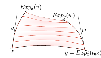
Figure 1. The quadrilateral in Lemma 5.1, defined by its two vertices $x,y$ and the corresponding tangent vectors $v,w$.

In the following result we verify that the geodesic distance between $Exp_{x}(v)$ and $Exp_{y}(w)$, which may be interpreted as the length of one of the sides in a curvlinear quadrilateral on $\mathcal{M}$ (with other two vertices $x$ and $y$, see Figure 1), deviates from the corresponding length of the side in a quadrilateral in $T_{x}\mathcal{M}$, only by controlled quadratic error terms:

Lemma 5.1.

In the above context, for every $s\in[0,1]$ there holds:

$$\begin{split}&L^{\prime}(s)=2t_{0}\Big{(}\Big{\langle}\frac{d}{ds}\gamma(s,t_{0}),\frac{d}{dt}\gamma(s,t_{0})\Big{\rangle}_{\gamma(s,t_{0})}-\Big{\langle}\frac{d}{ds}\gamma(s,0),\frac{d}{dt}\gamma(s,0)\Big{\rangle}_{\gamma(s,0)}\Big{)}\\ &L^{\prime\prime}(s)=2\Big{|}P_{\gamma(s,0),\gamma(s,t_{0})}P_{x,\gamma(s,0)}v-P_{y,\gamma(s,t_{0})}w\Big{|}^{2}+\mathcal{O}\big{(}t_{0}^{2}+s^{2}(|v|_{x}^{2}+|w|_{y}^{2})\big{)},\end{split}$$ (5.2)

where $P_{a,b}$ denotes the parallel transport along the unique geodesic connecting points $a,b\in\mathcal{M}$ with $d_{\mathcal{M}}(a,b)<\iota$. In particular, writing $y=Exp_{x}(t_{0}z)$ for some $z\in T_{x}\mathcal{M}$ with $|z|_{x}=1$, we have the following expansion, valid for $s\in[0,1]$:

$$\begin{split}L(s)&=t_{0}^{2}+2t_{0}s\langle P_{y,x}w-v,z\rangle_{x}+s^{2}|P_{y,x}w-v|_{x}^{2}+\mathcal{O}\big{(}s^{2}t_{0}^{2}+s^{4}(|v|_{x}^{2}+|w|_{y}^{2})\big{)}\\ &=\big{|}t_{0}z+s(P_{y,x}w-v)\big{|}_{x}^{2}+\mathcal{O}\big{(}s^{2}t_{0}^{2}+s^{4}(|v|_{x}^{2}+|w|_{y}^{2})\big{)}.\end{split}$$ (5.3)

The Landau symbol $\mathcal{O}$ above is uniform with respect to $x,y,v,w$ and depends only on $(\mathcal{M},g)$.

Proof.

1. Note first that by (5.1), we have:

$$L(s)=d_{\mathcal{M}}\big{(}\gamma(s,0),\gamma(s,t_{0})\big{)}\cdot\int_{0}^{t_{0}}\Big{|}\frac{d}{dt}\gamma(s,t)\Big{|}\;\mathrm{d}t=t_{0}\int_{0}^{t_{0}}\Big{|}\frac{d}{dt}\gamma(s,t)\Big{|}^{2}\;\mathrm{d}t.$$

We now differentiate in $s$, use the symmetry lemma in $\nabla_{\frac{d}{dt}\gamma}\frac{d}{ds}\gamma=\nabla_{\frac{d}{ds}\gamma}\frac{d}{dt}\gamma$, and the equation of geodesic $\nabla_{\frac{d}{dt}\gamma}\frac{d}{dt}\gamma=0$, to find that:

$$\begin{split}L^{\prime}(s)&=2t_{0}\int_{0}^{t_{0}}\Big{\langle}\frac{d}{dt}\gamma,\nabla_{\frac{d}{ds}\gamma}\frac{d}{dt}\gamma\Big{\rangle}\;\mathrm{d}t=2t_{0}\int_{0}^{t_{0}}\Big{\langle}\frac{d}{dt}\gamma,\nabla_{\frac{d}{dt}\gamma}\frac{d}{ds}\gamma\Big{\rangle}\;\mathrm{d}t\\ &=2t_{0}\int_{0}^{t_{0}}\frac{d}{dt}\Big{\langle}\frac{d}{dt}\gamma,\frac{d}{ds}\gamma\Big{\rangle}\;\mathrm{d}t=2t_{0}\Big{\langle}\frac{d}{dt}\gamma(s,t),\frac{d}{ds}\gamma(s,t)\Big{\rangle}\Big{|}_{t=0}^{t=t_{0}},\end{split}$$

as claimed in (5.2). To compute the second derivative of $L$, we observe that $\nabla_{\frac{d}{ds}\gamma}\frac{d}{ds}\gamma(s,0)=0$ and $\nabla_{\frac{d}{ds}\gamma}\frac{d}{ds}\gamma(s,t_{0})=0$, so that:

$$L^{\prime\prime}(s)=2t_{0}\Big{\langle}\nabla_{\frac{d}{ds}\gamma}\frac{d}{dt}\gamma(s,t),\frac{d}{ds}\gamma(s,t)\Big{\rangle}\Big{|}_{t=0}^{t=t_{0}}=2t_{0}\Big{\langle}\nabla_{\frac{d}{dt}\gamma}\frac{d}{ds}\gamma(s,t),\frac{d}{ds}\gamma(s,t)\Big{\rangle}\Big{|}_{t=0}^{t=t_{0}},$$

again in view of the symmetry lemma. Define the auxiliary vector field:

$$V(s,t)=\Big{(}1-\frac{t}{t_{0}}\Big{)}P_{\gamma(s,0),\gamma(s,t)}P_{x,\gamma(s,0)}v+\frac{t}{t_{0}}P_{\gamma(s,t_{0}),\gamma(s,t)}P_{y,\gamma(s,t_{0})}w\in T_{\gamma(s,t)}\mathcal{M}$$

for all $(s,t)\in[0,1]\times[0,t_{0}].$ Properties of parallel transport yield:

$$\nabla_{\frac{d}{dt}\gamma}V(s,t)=\frac{1}{t_{0}}\Big{(}P_{\gamma(s,t_{0}),\gamma(s,t)}P_{y,\gamma(s,t_{0})}w-P_{\gamma(s,0),\gamma(s,t)}P_{x,\gamma(s,0)}v\Big{)},$$

and since $V(s,0)=P_{x,\gamma(s,0)}v=\frac{d}{ds}\gamma(s,0)$ and $V(s,t_{0})=P_{y,\gamma(s,t_{0})}w=\frac{d}{ds}\gamma(s,t_{0})$, we obtain:

$$\begin{split}L^{\prime\prime}(s)&=2t_{0}\int_{0}^{t_{0}}\frac{d}{dt}\Big{\langle}\nabla_{\frac{d}{dt}\gamma}\frac{d}{ds}\gamma,V(s,t)\Big{\rangle}\;\mathrm{d}t\\ &=2\int_{0}^{t_{0}}\Big{\langle}\nabla_{\frac{d}{dt}\gamma}\frac{d}{ds}\gamma,P_{\gamma(s,t_{0}),\gamma(s,t)}P_{y,\gamma(s,t_{0})}w-P_{\gamma(s,0),\gamma(s,t)}P_{x,\gamma(s,0)}v\Big{\rangle}\;\mathrm{d}t\\ &\quad\qquad+2t_{0}\int_{0}^{t_{0}}\Big{\langle}\Big{(}\nabla_{\frac{d}{dt}\gamma}\Big{)}^{2}\frac{d}{ds}\gamma,V(s,t)\Big{\rangle}\;\mathrm{d}t\\ &=2\int_{0}^{t_{0}}\frac{d}{dt}\Big{\langle}\frac{d}{ds}\gamma,P_{\gamma(s,t_{0}),\gamma(s,t)}P_{y,\gamma(s,t_{0})}w-P_{\gamma(s,0),\gamma(s,t)}P_{x,\gamma(s,0)}v\Big{\rangle}\;\mathrm{d}t\\ &\quad\qquad+2t_{0}\int_{0}^{t_{0}}\Big{\langle}R\Big{(}\frac{d}{dt}\gamma,\frac{d}{ds}\gamma\Big{)}\frac{d}{dt}\gamma,V(s,t)\Big{\rangle}\;\mathrm{d}t\\ &\doteq 2A+2B.\end{split}$$ (5.4)

In the last step of (5.4), we used the fact that $\frac{d}{ds}\gamma(s,t)$ is a Jacobi field along the geodesic $t\mapsto\gamma(s,t)$. Below, we estimate separately the two terms $A$ and $B$.

2. For the first term in the right hand side of (5.4), we write:

$$\begin{split}A&=\Big{\langle}\frac{d}{ds}\gamma(s,t_{0}),P_{y,\gamma(s,t_{0})}w-P_{\gamma(s,0),\gamma(s,t_{0})}P_{x,\gamma(s,0)}v\Big{\rangle}\\ &\quad\qquad-\Big{\langle}\frac{d}{ds}\gamma(s,0),P_{\gamma(s,t_{0}),\gamma(s,t)}P_{y,\gamma(s,t_{0})}w-P_{x,\gamma(s,0)}v\Big{\rangle}\\ &=\Big{\langle}P_{y,\gamma(s,t_{0})}w,P_{y,\gamma(s,t_{0})}w-P_{\gamma(s,0),\gamma(s,t_{0})}P_{x,\gamma(s,0)}v\Big{\rangle}\\ &\quad\qquad-\Big{\langle}P_{\gamma(s,0),\gamma(s,t_{0})}P_{x,\gamma(s,0)}v,P_{y,\gamma(s,t_{0})}w-P_{\gamma(s,0),\gamma(s,t_{0})}P_{x,\gamma(s,0)}v\Big{\rangle}\\ &=\Big{|}P_{y,\gamma(s,t_{0})}w-P_{\gamma(s,0),\gamma(s,t_{0})}P_{x,\gamma(s,0)}v\Big{|}^{2}.\end{split}$$

For the second term, we observe that:

$$\begin{split}|B|&\leq Ct_{0}^{2}\sup_{t\in[0,t_{0}]}\Big{|}R\Big{(}\frac{d}{dt}\gamma,\frac{d}{ds}\gamma\Big{)}\frac{d}{dt}\gamma(s,t)\Big{|}\cdot|V(s,t)|\\ &\leq Ct_{0}^{2}\sup_{t\in[0,t_{0}]}\Big{(}\Big{|}\frac{d}{dt}\gamma(s,t)\Big{|}^{2}\cdot\Big{|}\frac{d}{ds}\gamma(s,t)\Big{|}\cdot|V(s,t)|\Big{)}\\ &\leq Cd_{\mathcal{M}}\big{(}\gamma(s,0),\gamma(s,t_{0})\big{)}^{2}\cdot\big{(}|v|+|w|\big{)}\cdot\sup_{t\in[0,t_{0}],s\in[0.1]}\Big{|}\frac{d}{ds}\gamma(s,t)\Big{|}\\ &\leq Ct_{0}^{2}\big{(}|v|+|w|\big{)}+Cs^{2}\big{(}|v|+|w|\big{)}^{3},\end{split}$$

because:

$$d_{\mathcal{M}}\big{(}\gamma(s,0),\gamma(s,t_{0})\big{)}\leq d_{\mathcal{M}}(\gamma(s,0),x)+d_{\mathcal{M}}(x,y)+d_{\mathcal{M}}(y,\gamma(s,t_{0}))=t_{0}+s\big{(}|v|_{x}+|w|_{y}\big{)},$$

and because $\big{|}\frac{d}{ds}\gamma(s,t)\big{|}\leq C$ for all $(s,t)\in[0,1]\times[0,t_{0}]$. This last assertion, following from general properties of the exponential map, will be justified in Proposition 5.2. The proof of (5.2) is complete.

3. To show (5.3), we Taylor expand $L$ at $0$ to get:

$$L(s)=L(0)+sL^{\prime}(0)+\frac{s^{2}}{2}L^{\prime\prime}(\bar{s})\qquad\mbox{ for some }\bar{s}\in[0,s],$$

where we noted that $L(0)=t_{0}$ and $L^{\prime}(0)=2t_{0}\big{(}\langle w,P_{x,y}z\rangle-\langle v,z\rangle\big{)}=2t_{0}\langle P_{y,x}w-v,z\rangle$ by (5.2). On the other hand:

$$\begin{split}P_{y,\gamma(\bar{s},t_{0})}&w-P_{\gamma(\bar{s},0),\gamma(\bar{s},t_{0})}P_{x,\gamma(\bar{s},0)}v\\ &=P_{y,\gamma(\bar{s},t_{0})}\big{(}w-P_{x,y}v\big{)}+\Big{(}P_{y,\gamma(\bar{s},t_{0})}P_{x,y}v-P_{\gamma(\bar{s},0),\gamma(\bar{s},t_{0})}P_{x,\gamma(\bar{s},0)}v\Big{)}.\end{split}$$ (5.5)

The first vector in the right hand side above has length $|w-P_{x,y}v|_{y}=|P_{y,x}w-v|_{x}$. The second vector compares the parallel transport of $v$ from $x$ to $\gamma(\bar{s},t_{0})$ by two different routes, and has length equal to:

$$\big{|}v-P_{y,x}P_{\gamma(\bar{s},t_{0}),y}P_{\gamma(\bar{s},0),\gamma(\bar{s},t_{0})}P_{x,\gamma(\bar{s},0)}v\big{|}_{x}\leq C\big{(}t_{0}^{2}+\bar{s}^{2}(|v|^{2}_{x}+|w|_{y}^{2})\big{)},$$

as easily seen, for example, from equations of parallel transport written in normal coordinates centered at $x$ (see section A.3). By (5.2) and (5.5), for every $\bar{s}\in[0,s]$ we thus get:

$$\begin{split}\frac{1}{2}L^{\prime\prime}(\bar{s})&=\Big{|}P_{y,\gamma(\bar{s},t_{0})}w-P_{\gamma(\bar{s},0),\gamma(\bar{s},t_{0})}P_{x,\gamma(\bar{s},0)}v\Big{|}^{2}+\mathcal{O}\big{(}t_{0}^{2}+s^{2}(|v|^{2}_{x}+|w|_{y}^{2})\big{)}\\ &=|P_{y,x}w-v|^{2}+\mathcal{O}\big{(}t_{0}^{2}+s^{2}(|v|^{2}_{x}+|w|_{y}^{2})\big{)},\end{split}$$

which ends the proof of (5.3) and of the Lemma.   

In the argument above we used the following observation:

Proposition 5.2.

In the above context, there holds:

$$\Big{|}\frac{d}{ds}\gamma(s,t)\Big{|}=\mathcal{O}(1)\qquad\mbox{ for all }(s,t)\in[0,1]\times[0,t_{0}],$$

where the bound $\mathcal{O}$ depends only on $(\mathcal{M},g)$.

Proof.

Recall (see section A.2) that given $x\in\mathcal{M}$ and $v\in T_{x}\mathcal{M}$ with $|v|_{x}<\iota$, we have $\psi(x,v)\doteq\big{(}x,Exp_{x}(v)\big{)}\in\mathcal{M}\times\mathcal{M}$, and that the mapping $\psi$ is a smooth diffeomorphism onto its image. For $x,y,v,w$ as in the definition of the Levi-Cività quadrilateral, and for all $s\in[0,1]$, $t\in[0,d_{\mathcal{M}}(x,y)]$, we observe that the following composite mapping:

$$\begin{split}(x,y,v,w,s,&\;t)\mapsto\Big{(}Exp_{x}(sv),Exp_{y}(sw),\frac{t}{d_{\mathcal{M}}(x,y)}\Big{)}\\ &~{}{\overset{(\psi^{-1},id)}{\mapsto}}\Big{(}Exp_{x}(sv),Exp^{-1}_{Exp_{x}(sv)}\big{(}Exp_{y}(sw)\big{)},\frac{t}{d_{\mathcal{M}}(x,y)}\Big{)}\\ &\quad\mapsto\Big{(}Exp_{x}(sv),\frac{t}{d_{\mathcal{M}}(x,y)}Exp^{-1}_{Exp_{x}(sv)}\big{(}Exp_{y}(sw)\big{)}\Big{)}\\ &~{}\mbox{ }\;\mbox{ }{\overset{\psi}{\mapsto}}\Big{(}Exp_{x}(sv),Exp_{Exp_{x}(sv)}\Big{(}\frac{t}{d_{\mathcal{M}}(x,y)}Exp^{-1}_{Exp_{x}(sv)}\big{(}Exp_{y}(sw)\big{)}\Big{)}\Big{)}\\ &\quad=\big{(}Exp_{x}(sv),\gamma(s,t)\big{)}\end{split}$$

is smooth in $s$, independently of $x,y,v,w$ and of the scaled parameter $\frac{t}{d_{\mathcal{M}}(x,y)}\in[0,1]$. In particular, $\frac{d}{ds}\gamma(s,t)$ is uniformly bounded, as claimed.   

6. The averaging operators ${\mathcal{A}}_{\varepsilon}$, ${\bar{\mathcal{A}}}_{\varepsilon}$ and their mean value expansions

In this section, we work under the following hypothesis, that are less restrictive than (H1):

$$\left[\quad\;\;\mbox{\begin{minipage}{372.73126pt}\vspace{1mm} \begin{itemize}[leftmargin=*] \par\itemize@item@[(i)] $(\mathcal{M},g)$ is a smooth, compact, boundaryless, connected and orientable manifold of dimension $m$,\vspace{1mm} \par\itemize@item@[(ii)] $\rho\in\mathcal{C}^{2}(\mathcal{M})$ is a positive scalar field, \vspace{1mm} \par\itemize@item@[(iii)] $\eta:[0,1]\to\mathbb{R}$ is Borel regular, nonnegative, satisfying $\int_{B(0,1)\subset\mathbb{R}^{m}}\eta(|w|)\;\mathrm{d}w=1$. It yields the positive coefficient: $\sigma_{\eta}=\int_{B(0,1)}\langle w,e_{1}\rangle^{2}\eta(|w|)\;\mathrm{d}w.$ \vspace{1mm} \par\end{itemize} \end{minipage}}\;\;\,\right]$$ (H2)

We consider the differential operator (see section A.3):

$$Af\doteq\frac{1}{\rho^{2}}Div\big{(}\rho^{2}\nabla^{*}f)=\Delta f+2\langle\nabla^{*}f,\nabla^{*}(\log\rho)\rangle_{x},$$

where $\Delta$ is the unweighted Laplace-Beltrami operator. In turn, $A$ is a scaled version of $\Delta_{\mathcal{M}}$ as defined in (2.2). The purpose of this section is to discuss two families of “averaging” operators, relative to the chosen $\eta$, that approximate $A$ when the domains of averaging shrink to a point.

For a bounded, Borel function $f:\mathcal{M}\to\mathbb{R}$ and $\varepsilon\ll 1$, the first averaging operator (already encountered in section 4.3) is given via integrating on the geodesic ball $B_{\mathcal{M}}(x,\varepsilon)$:

$$\begin{split}\mathcal{A}_{\varepsilon}f(x)&=\frac{1}{d_{\varepsilon}(x)}\int_{B_{\mathcal{M}}(x,\varepsilon)}\frac{1}{\varepsilon^{m}}\eta\Big{(}\frac{d_{\mathcal{M}}(x,y)}{\varepsilon}\Big{)}f(y)\rho(y)\;\;\mathrm{d{{Vol}}}_{\mathcal{M}}(y)\\ &\mbox{ where }~{}~{}d_{\varepsilon}(x)=\int_{B_{\mathcal{M}}(x,\varepsilon)}\frac{1}{\varepsilon^{m}}\eta\Big{(}\frac{d_{\mathcal{M}}(x,y)}{\varepsilon}\Big{)}\rho(y)\;\;\mathrm{d{{Vol}}}_{\mathcal{M}}(y)\quad\mbox{ for all }x\in\mathcal{M}.\end{split}$$

The second operator involves integrating on the unit ball $B(0,1)\subset T_{x}\mathcal{M}\simeq\mathbb{R}^{m}$ and interpreting the integrated quantities in the normal coordinates centered at a given point $x$:

$$\bar{\mathcal{A}}_{\varepsilon}f(x)=\int_{B(0,1)}\eta(|w|)\Big{(}1+\varepsilon\big{\langle}w,\nabla(\log\rho)(0)\big{\rangle}\Big{)}f(\varepsilon w)\;\mathrm{d}w\quad\mbox{ for all }x\in\mathcal{M}.$$

It is not hard to observe that both functions $\mathcal{A}_{\varepsilon}f,\bar{\mathcal{A}}_{\varepsilon}f:\mathcal{M}\to\mathbb{R}$ are continuous and bounded by $C\sup_{x\in\mathcal{M}}|f(x)|$ where the constant $C$ depends only on $\rho$. The relation of $\mathcal{A}_{\varepsilon},\bar{\mathcal{A}}_{\varepsilon}$ to $A$ is revealed in the next result, which may be also deduced from the proof of [13, Lemma 3.5].

Theorem 6.1.

For every $f\in\mathcal{C}^{3}(\mathcal{M})$ there holds:

$$\mathcal{A}_{\varepsilon}f(x),~{}\bar{\mathcal{A}}_{\varepsilon}f(x)=f(x)+\frac{1}{2}\sigma_{\eta}\varepsilon^{2}Af(x)+\mathcal{O}(\varepsilon^{3})\|\nabla f\|_{\mathcal{C}^{2}(\mathcal{M})}\qquad\mbox{ for all }x\in\mathcal{M},$$

where the Landau symbol $\mathcal{O}$ depends only on $(\mathcal{M},g)$ and $\rho$, and where $\sigma_{\eta}$ is as in (H2).

Proof.

1. We fix $x\in\mathcal{M}$ and calculate in normal coordinates centered at $x$ (recall that in these coordinates $Exp_{x}(\varepsilon w)\in\mathcal{M}$ corresponds to $\varepsilon w\in B(0,\varepsilon)\in T_{x}\mathcal{M}\simeq\mathbb{R}^{m})$:

$$\begin{split}\mathcal{A}_{\varepsilon}f(x)-f(x)&=\frac{1}{d_{\varepsilon}(x)}\int_{B_{\mathcal{M}}(x,\varepsilon)}\frac{1}{\varepsilon^{m}}\eta\Big{(}\frac{d_{\mathcal{M}}(x,y)}{\varepsilon}\Big{)}\big{(}f(y)-f(x)\big{)}\rho(y)\;\mathrm{d{{Vol}}}_{\mathcal{M}}(y)\\ &=\frac{1}{d_{\varepsilon}(x)}\int_{B(0,1)}\eta(|w|)\big{(}f(\varepsilon w)-f(0)\big{)}\rho(\varepsilon w)\sqrt{\det[g_{ij}(\varepsilon w)]}\;\mathrm{d}w,\end{split}$$

where the last integration is on the Euclidean ball $B(0,1)\subset\mathbb{R}^{m}$. Similarly, we have: $d_{\varepsilon}(x)=\int_{B(0,1)}\eta(|w|)\rho(\varepsilon w)\sqrt{\det[g_{ij}(\varepsilon w)]}\;\mathrm{d}w$. Since in normal coordinates $g_{ij}(\varepsilon w)=\delta_{ij}+\mathcal{O}(\varepsilon^{2})$, it immediately follows that: $\sqrt{\det[g_{ij}(\varepsilon w)]}=1+\mathcal{O}(\varepsilon^{2})$. Taylor expanding $\rho\circ Exp_{x}$, we now get:

$$\begin{split}d_{\varepsilon}(x)=\int_{B(0,1)}\eta(|w|)\big{(}\rho(0)+\varepsilon\langle\nabla\rho,w\rangle+\mathcal{O}(\varepsilon^{2})\big{)}\big{(}1+\mathcal{O}(\varepsilon^{2})\big{)}\;\mathrm{d}w=\rho(0)+\mathcal{O}(\varepsilon^{2}),\end{split}$$ (6.1)

and thus $\frac{1}{d_{\varepsilon}(x)}=\frac{1}{\rho(0)}+\mathcal{O}(\varepsilon^{2})$. Similarly, Taylor expanding $f\circ Exp_{x}$ we obtain:

$$\begin{split}d_{\varepsilon}(x)&\Big{(}\mathcal{A}_{\varepsilon}f(x)-f(x)\Big{)}=\int_{B(0,1)}\eta(|w|)\Big{(}\varepsilon\langle\nabla f(0),w\rangle+\frac{\varepsilon^{2}}{2}\langle\nabla^{2}f(0):w^{\otimes 2}\rangle+\mathcal{O}(\varepsilon^{3})\|\nabla^{3}f\|_{\mathcal{C}^{0}(\mathcal{M})}\Big{)}\\ &\qquad\qquad\qquad\qquad\cdot\big{(}\rho(0)+\varepsilon\langle\nabla\rho(0),w\rangle+\mathcal{O}(\varepsilon^{2})\big{)}\cdot(1+\mathcal{O}(\varepsilon^{2}))\;\mathrm{d}w\\ &=\varepsilon\rho(0)\int_{B(0,1)}\eta(|w|)\langle\nabla f(0),w\rangle\;\mathrm{d}w\\ &\quad+\frac{\varepsilon^{2}}{2}\rho(0)\int_{B(0,1)}\eta(|w|)\Big{(}\langle\nabla^{2}f(0):w^{\otimes 2}\rangle+2\langle\nabla f(0),w\rangle\cdot\Big{\langle}\frac{\nabla\rho(0)}{\rho(0)},w\Big{\rangle}\Big{)}\;\mathrm{d}w\\ &\quad+\mathcal{O}(\varepsilon^{3})\big{(}\|\nabla f\|_{\mathcal{C}^{0}(\mathcal{M})}+\|\nabla^{2}f\|_{\mathcal{C}^{0}(\mathcal{M})}+\|\nabla^{3}f\|_{\mathcal{C}^{0}(\mathcal{M})}\big{)}\\ &=\varepsilon^{2}\rho(0)\Big{\langle}\nabla^{2}f(0)+2\nabla f(0)\otimes\nabla(\log\rho)(0):\frac{1}{2}\int_{B(0,1)}\eta(|w|)w^{\otimes 2}\;\mathrm{d}w\Big{\rangle}+\mathcal{O}(\varepsilon^{3})\|\nabla f\|_{\mathcal{C}^{2}(\mathcal{M})}.\end{split}$$

Since $\int_{B(0,1)}\eta(|w|)w^{\otimes 2}\;\mathrm{d}w=\sigma_{\eta}Id_{m}$, it follows that:

$$\mathcal{A}_{\varepsilon}f(x)-f(x)=\frac{1}{2}\varepsilon^{2}\sigma_{\eta}\Big{(}\Delta f+2\langle\nabla f(0),\nabla(\log\rho)(0)\rangle\Big{)}+\mathcal{O}(\varepsilon^{3})\|\nabla f\|_{\mathcal{C}^{2}(\mathcal{M})},$$

proving the claim.

2. For the averaging operator $\bar{\mathcal{A}}_{\varepsilon}$, we likewise expand and calculate in normal coordinates:

$$\begin{split}&\bar{\mathcal{A}}_{\varepsilon}f(x)-f(x)=\int_{B(0,1)}\eta(|w|)\Big{(}1+\varepsilon\langle w,\nabla(\log\rho)(0)\rangle\Big{)}\\ &\qquad\qquad\qquad\qquad\qquad\cdot\Big{(}\varepsilon\langle\nabla f(0),w\rangle+\frac{\varepsilon^{2}}{2}\langle\nabla^{2}f(0):w^{\otimes 2}\rangle+\mathcal{O}(\varepsilon^{3})\|\nabla^{3}f\|_{\mathcal{C}^{0}(\mathcal{M})}\Big{)}\;\mathrm{d}w\\ &\quad=\frac{\varepsilon^{2}}{2}\rho(0)\int_{B(0,1)}\eta(|w|)\Big{(}\langle\nabla^{2}f(0):w^{\otimes 2}\rangle+2\langle\nabla f(0),w\rangle\cdot\langle\nabla(\log\rho)(0),w\rangle\Big{)}\;\mathrm{d}w+\mathcal{O}(\varepsilon^{3})\|\nabla f\|_{\mathcal{C}^{1}}\\ &\quad=\frac{1}{2}\varepsilon^{2}\sigma_{\eta}\Big{(}\Delta f+2\langle\nabla f(0),\nabla(\log\rho)(0)\rangle\Big{)}+\mathcal{O}(\varepsilon^{3})\|\nabla^{2}f\|_{\mathcal{C}^{1}(\mathcal{M})}.\end{split}$$

The proof is complete.   

Remark 6.2.

(i) When $\eta\equiv\frac{1}{|B(0,1)|}$, then $\sigma_{\eta}=\fint_{B(0,1)}\langle w,e_{1}\rangle^{2}\;\mathrm{d}w=\frac{1}{2(m+2)}$, so that:

$$\frac{1}{\int_{B_{\mathcal{M}}(x,\varepsilon)}\rho(y)\;\mathrm{d{{Vol}}}_{\mathcal{M}}(y)}\cdot\int_{B_{\mathcal{M}}(x,\varepsilon)}f(y)\rho(y)\;\mathrm{d{{Vol}}}_{\mathcal{M}}(y)=f(x)+\frac{\varepsilon^{2}}{2(m+2)}\Delta f(x)+\mathcal{O}(\varepsilon^{3})\quad\mbox{ as }\varepsilon\to 0.$$

This observation is consistent with the mean-value expansion, valid for $\rho\equiv C$ and $A=\Delta$:

$$\fint_{B_{\mathcal{M}}(x,\varepsilon)}f(y)\;\mathrm{d{{Vol}}}_{\mathcal{M}}(y)=f(x)+\frac{\varepsilon^{2}}{2(m+2)}\Delta f(x)+\mathcal{O}(\varepsilon^{3}).$$

The above expansion is, in turn, the quantitative version of one of the equivalent properties of harmonic functions defined on $\mathcal{U}\subset\mathbb{R}^{m}$, namely: $f(x)=\fint_{B(x,r)}f(y)\;\mathrm{d}y$ for all $\bar{B}(x,r)\subset\mathcal{U}$.

(ii) The relation of the averaging operator $\mathcal{A}_{\varepsilon}$ to $\Delta_{\varepsilon}$ defined in (1.5) is:

$$\Delta_{\varepsilon}f(x)=-d_{\varepsilon}(x)\cdot\frac{\mathcal{A}_{\varepsilon}f(x)-f(x)}{\varepsilon^{2}}.$$

We may directly estimate the difference of the two studied averages:

Lemma 6.3.

For every Borel, bounded function $f:\mathcal{M}\to\mathbb{R}$ there holds:

$$\big{|}\mathcal{A}_{\varepsilon}f(x)-\bar{\mathcal{A}}_{\varepsilon}f(x)\big{|}=\mathcal{O}(\varepsilon^{2})\|f\|_{L^{\infty}(B_{\mathcal{M}}(x,\varepsilon))}\qquad\mbox{ for all }x\in\mathcal{M}.$$

When $f$ is continuous, with the modulus of continuity $\omega(f,\cdot)$, then:

$$\big{|}\mathcal{A}_{\varepsilon}f(x)-\bar{\mathcal{A}}_{\varepsilon}f(x)\big{|}=\mathcal{O}(\varepsilon^{2})\cdot\omega(f,\varepsilon)\qquad\mbox{ for all }x\in\mathcal{M}.$$

In both bounds, the quantity $\mathcal{O}$ depends only on $(\mathcal{M},g)$ and $\rho$.

Proof.

1. For a fixed $x\in\mathcal{M}$, we compute in normal coordinates centered at $x$:

$$\begin{split}&\mathcal{A}_{\varepsilon}f(x)-\bar{\mathcal{A}}_{\varepsilon}f(x)\\ &=\frac{1}{d_{\varepsilon}(x)}\int_{B(0,1)}\eta(|w|)f(\varepsilon w)\Big{(}\rho(\varepsilon w)\sqrt{\det[g_{ij}(\varepsilon w)]}-d_{\varepsilon}(x)\big{(}1+\varepsilon\langle w,\nabla(\log\rho)(0)\rangle\big{)}\Big{)}\;\mathrm{d}w.\end{split}$$ (6.2)

We recall that $[g_{ij}]_{i,j=1\ldots m}$ denotes the Grammian matrix in normal coordinates and that, as before, $\varepsilon w$ is identified with $Exp_{x}(\varepsilon w)$. Observe that by (A.5) we get:

$$\begin{split}\det[g_{ij}(\varepsilon w)]&=\det\big{[}\delta_{ij}-\frac{\varepsilon^{2}}{3}R^{i}_{kjs}(0)w^{k}w^{s}+\mathcal{O}(\varepsilon^{3})\big{]}_{i,j=1\ldots m}\\ &=1-\frac{\varepsilon^{2}}{3}R_{kis}^{i}(0)w^{k}w^{s}+\mathcal{O}(\varepsilon^{3})=1-\frac{\varepsilon^{2}}{3}\big{\langle}[Ric_{ij}(0)]:w^{\otimes 2}\big{\rangle}+\mathcal{O}(\varepsilon^{3}),\end{split}$$

where $Ric$ denotes the Ricci curvature tensor, here computed at $x$. Consequently:

$$\sqrt{\det[g_{ij}(\varepsilon w)]}=1-\frac{\varepsilon^{2}}{6}\big{\langle}[Ric_{ij}(0)]:w^{\otimes 2}\big{\rangle}+\mathcal{O}(\varepsilon^{3}),$$

allowing to improve (6.1) to a more precise expansion:

$$\begin{split}d_{\varepsilon}(x)&=\int_{B(0,1)}\eta(|w|)\Big{(}\rho(0)+\varepsilon\langle\nabla\rho,w\rangle+\frac{\varepsilon^{2}}{2}\langle\nabla^{2}\rho(0):w^{\otimes 2}\rangle+o(\varepsilon^{2})\Big{)}\\ &\qquad\qquad\cdot\Big{(}1-\frac{\varepsilon^{2}}{6}\langle[Ric_{ij}(0)]:w^{\otimes 2}\big{\rangle}+\mathcal{O}(\varepsilon^{3})\Big{)}\;\mathrm{d}w\\ &=\rho(0)+\varepsilon^{2}\Big{\langle}\frac{1}{2}\int_{B(0,1)}\eta(|w|)w^{\otimes 2}\;\mathrm{d}w:\nabla^{2}\rho(0)-\frac{1}{3}\rho(0)[Ric_{ij}(0)]\Big{\rangle}+o(\varepsilon^{2})\\ &=\rho(0)+\frac{1}{2}\sigma_{\eta}\varepsilon^{2}\Big{(}\Delta\rho(0)-\frac{1}{3}\rho(0)R(0)\Big{)}+o(\varepsilon^{2}).\end{split}$$ (6.3)

Here, $R(0)$ denotes the scalar curvature at $x$ and $\Delta$ is the unweighted Laplacian.

2. In conclusion, the integration factor in (6.2) is:

$$\begin{split}\rho(\varepsilon w)&\sqrt{\det[g_{ij}(\varepsilon w)]}-d_{\varepsilon}(x)\big{(}1+\varepsilon\langle w,\nabla(\log\rho)(0)\rangle\big{)}\\ &=\Big{(}\rho(0)+\varepsilon\langle\nabla\rho(0),w\rangle+\frac{\varepsilon^{2}}{2}\langle\nabla^{2}\rho(0):w^{\otimes 2}\rangle+o(\varepsilon^{2})\Big{)}\cdot\Big{(}1-\frac{\varepsilon^{2}}{6}\langle[Ric_{ij}(0)]:w^{\otimes 2}\big{\rangle}+\mathcal{O}(\varepsilon^{3})\Big{)}\\ &\quad-\Big{(}\rho(0)+\kappa_{\eta}\varepsilon^{2}\big{(}\Delta\rho(0)-\frac{1}{3}\rho(0)R(0)\big{)}+o(\varepsilon^{2})\Big{)}\cdot\big{(}1+\varepsilon\langle w,\nabla(\log\rho)(0)\rangle\big{)}\\ &=\frac{\varepsilon^{2}}{2}\Big{\langle}\nabla^{2}\rho(0)-\frac{1}{3}\rho(0)[Ric_{ij}(0)]:w^{\otimes 2}\Big{\rangle}-\frac{1}{2}\sigma_{\eta}\varepsilon^{2}\big{(}\Delta\rho(0)-\frac{1}{3}\rho(0)R(0)\big{)}+o(\varepsilon^{2}).\end{split}$$

Since the $\varepsilon^{2}$-order term above integrates to $0$, against $\eta(|w|)$ on $B(0,1)$, we see that for continuous $f$, the difference in (6.2) becomes:

$$\begin{split}\mathcal{A}_{\varepsilon}&f(x)-\bar{\mathcal{A}}_{\varepsilon}f(x)\\ &=\frac{\varepsilon^{2}}{d_{\varepsilon}(x)}\int_{B(0,1)}\eta(|w|)\big{(}f(\varepsilon w)-f(0)\big{)}\\ &\qquad\qquad\cdot\Big{(}\frac{1}{2}\Big{\langle}\nabla^{2}\rho(0)-\frac{1}{3}\rho(0)[Ric_{ij}(0)]:w^{\otimes 2}\Big{\rangle}-\frac{1}{2}\sigma_{\eta}\Delta\rho(0)-\frac{1}{6}\sigma_{\eta}\rho(0)R(0)+o(1)\Big{)}\;\mathrm{d}w\\ &=\mathcal{O}(\varepsilon^{2})\cdot\omega(f,\varepsilon).\end{split}$$

The estimate for bounded $f$ is a consequence of the first equality above and of (6.3).   

7. A biased random walk modeled on the averaging operator $\bar{\mathcal{A}}_{\varepsilon}$

In this section, we work under hypothesis (H2). We introduce a discrete, $\mathcal{M}$-valued process whose dynamic programming principle reflects the averaging operation in $\bar{\mathcal{A}}_{\varepsilon}$. Ultimately, this process $\{X_{n}^{\varepsilon,x_{0}}\}_{n=0}^{\infty}$ will serve for tracking the values of a solution $f$ in function of its average.

7.1. The local isometry field $Q$

We start by the following easy observation:

Lemma 7.1.

For a given $x\in\mathcal{M}$, let $Q$ be a linear isometry of $T_{x}\mathcal{M}$, such that for some $e\in T_{x}\mathcal{M}$ with $|e|_{x}=1$ there holds:

$$|\nabla(\log\rho)(x)|_{x}Qe=\nabla(\log\rho)(x).$$ (7.1)

Then, for every bounded, Borel $f:\mathcal{M}\to\mathbb{R}$ we have:

$$\begin{split}\bar{\mathcal{A}}_{\varepsilon}f(x)&=\big{(}1-\varepsilon|\nabla(\log\rho)(0)|\big{)}\int_{B(0,1)}\eta(|w|)f(\varepsilon w)\;\mathrm{d}w\\ &\quad+\varepsilon|\nabla(\log\rho)(0)|\int_{B(0,1)}\eta(|w|)(1+\langle w,e\rangle)f(\varepsilon Qw)\;\mathrm{d}w,\end{split}$$

where the formula above is written in the normal coordinates centered at $x$, and the integration is on $B(0,1)\subset\mathbb{R}^{m}\simeq T_{x}\mathcal{M}$.

Proof.

We change the variable in the second term, to obtain:

$$\begin{split}\varepsilon|&\nabla(\log\rho)(0)|\int_{B(0,1)}\eta(|w|)(1+\langle w,e\rangle)f(\varepsilon Qw)\;\mathrm{d}w\\ &=\varepsilon|\nabla(\log\rho)(0)|\int_{B(0,1)}\eta(|w|)(1+\langle w,Qe\rangle)f(\varepsilon w)\;\mathrm{d}w\\ &=\varepsilon|\nabla(\log\rho)(0)|\int_{B(0,1)}\eta(|w|)f(\varepsilon Qw)\;\mathrm{d}w+\varepsilon\int_{B(0,1)}\eta(|w|)\langle w,\nabla(\log\rho)(0)\rangle)f(\varepsilon w)\;\mathrm{d}w.\end{split}$$

Summing with $\big{(}1-\varepsilon|\nabla(\log\rho)(0)|\big{)}\int_{B(0,1)}\eta(|w|)f(\varepsilon w)\;\mathrm{d}w$, we get $\bar{\mathcal{A}}_{\varepsilon}f(x)$, as claimed.   

In what follows, we will define a specific field of isometries $Q$ on a small geodesic ball $B_{\mathcal{M}}(x_{0},\iota)$. The field $Q$ will be Borel-regular and will satisfy (7.1) for the chosen unit vectors $e_{1}(x)=P_{x_{0},x}e_{1}\in T_{x}\mathcal{M}$. More precisely, given the normal coordinates on $B_{\mathcal{M}}(x_{0},\iota)$ centered at $x_{0}\in\mathcal{M}$, we write $\big{\{}e_{i}=\frac{\partial}{\partial x^{i}}_{\mid x_{0}}\big{\}}_{i=1}^{m}$ for the orthonormal frame that spans $T_{x_{0}}\mathcal{M}\simeq\mathbb{R}^{m}$. Then, at each $x\in B_{\mathcal{M}}(x_{0},\iota)$ we consider the parallel transported orthonormal frame $\big{\{}e_{i}(x)\doteq P_{x_{0},x}e_{i}\big{\}}_{i=1}^{m}$ in $T_{x}\mathcal{M}\simeq\mathbb{R}^{m}$.

Define the spherical cups (interpreted as subsets of $T_{x_{0}}\mathcal{M}$):

$$\begin{split}S_{0}^{\pm}=\Big{\{}w\in&\mathbb{R}^{m};~{}|w|=1\mbox{ and }\langle w,\pm e_{1}\rangle>\cos\frac{8\pi}{9}\Big{\}}\\ &\supset S_{1}^{\pm}=\Big{\{}w\in\mathbb{R}^{m};~{}|w|=1\mbox{ and }\langle w,\pm e_{1}\rangle>\cos\frac{5\pi}{9}\Big{\}},\end{split}$$

and fix one rotation $Q_{0}\in SO(m)$ satisfying:

$$Q_{0}(S_{j}^{-})=S_{j}^{+}\quad\mbox{ for }j=0,1\qquad\mbox{with }Q_{0}(-e_{1})=e_{1}.$$

Let $\bar{Q}:S_{0}^{+}\to SO(m)$ be a smooth map such that:

$$\bar{Q}(e)e_{1}=e\qquad\mbox{ for all }e\in S_{0}^{+}.$$

For $x\in B_{\mathcal{M}}(x_{0},\iota)$, using the notation $\xi(x)=\frac{\nabla(\log\rho(x)}{|\nabla(\log\rho(x)|_{x}}$ whenever defined, we set $Q(x)\in SO(T_{x}\mathcal{M})$ as follows:

$$Q(x)=\left\{\begin{array}[]{ll}P_{x_{0},x}\circ\bar{Q}(P_{x,x_{0}}\xi(x))\circ P_{x,x_{0}}&\mbox{if }P_{x,x_{0}}\xi(x)\in S_{1}^{+}\\ P_{x_{0},x}\circ Q_{0}^{T}\bar{Q}\big{(}Q_{0}\cdot P_{x,x_{0}}\xi(x)\big{)}\circ P_{x,x_{0}}&\mbox{if }P_{x,x_{0}}\xi(x)\in S_{1}^{-}\setminus S_{1}^{+}\\ Id_{T_{x}\mathcal{M}}&\mbox{otherwise.}\end{array}\right.$$ (7.2)

Clearly, property (7.1) holds for each $x$, with $e=e_{1}(x)=P_{x_{0},x}e_{1}$.

7.2. The probability spaces and the discrete process

We denote the following probability spaces on the collection of Borel subsets of $B(0,1)\subset\mathbb{R}^{m}$:

$$\Omega_{1}=\Big{(}B(0,1),\mbox{Borel},\eta(|w|)\;\mathrm{d}w\Big{)},\qquad\bar{\Omega}_{1}=\Big{(}B(0,1),\mbox{Borel},\big{(}1+\langle\bar{w},e_{1}\rangle\big{)}\eta(|\bar{w}|)\;\mathrm{d}\bar{w}\Big{)},$$

together with the probability space $\big{(}(0,1),\mbox{Borel},\;\mathrm{d}b\big{)}$. The product measure on $\Omega_{1}\times\bar{\Omega}_{1}\times(0,1)$ will be denoted $\nu_{1}$. We also consider the infinite product measure space $(\Omega,\mathcal{F},\nu)$:

$$\begin{split}\Omega&=\big{(}\Omega_{1}\times\bar{\Omega}_{1}\times(0,1)\big{)}^{\mathbb{N}}\\ &=\Big{\{}\omega=(w_{i},\bar{w}_{i},b_{i})_{i=1}^{\infty}\mbox{ with }w_{i},\bar{w}_{i}\in B(0,1)\mbox{ and }b_{i}\in(0,1)\mbox{ for all }i=1\ldots\infty\Big{\}}.\end{split}$$

The product $\sigma$-algebra $\mathcal{F}$ has the natural filtration by $\{\mathcal{F}_{n}\}_{n=0}^{\infty}$, each generated by finite products (identified as subsets of $\mathcal{F}$) of $n$ Borel subsets of $B(0,1)^{2}\times(0,1)$. We also write $\mathcal{F}_{0}=\{\emptyset,\Omega\}$.

Equivalently, $\{w_{i}\}_{i=1}^{\infty}$, $\{\bar{w}_{i}\}_{i=1}^{\infty}$ are collections of independent random variables sampled from the distributions on $T_{x_{0}}\mathcal{M}\simeq\mathbb{R}^{m}$ with respective densities: $\big{(}\eta\mathds{1}_{[0,1]}\big{)}(|w|)$ and $(1+\langle\bar{w},e_{1}\rangle)\big{(}\eta\mathds{1}_{[0,1]}\big{)}(|w|)$, while $\{b_{i}\}_{i=1}^{\infty}$ are i.i.d. samples uniformly distributed on the interval $(0,1)$.

Fix $x_{0}\in\mathcal{M}$, $\varepsilon\in(0,\frac{\iota}{2})$, and some sufficiently small radius $r<\frac{\iota}{2}$. We introduce the sequence of random variables $\{X_{n}^{\varepsilon,x_{0}}:\Omega\to\mathcal{M}\}_{n=0}^{\infty}$, via the recursive formula:

$$\begin{split}&X_{0}\equiv x_{0}\\ &X_{n+1}=\left\{\begin{array}[]{ll}X_{n}&\mbox{if }X_{n}\not\in B_{\mathcal{M}}(x_{0},r)\\ Exp_{X_{n}}(\varepsilon P_{x_{0},X_{n}}w_{n+1})&\mbox{otherwise and if }b_{n+1}\geq\varepsilon|\nabla(\log\rho)(X_{n})|_{X_{n}}\\ Exp_{X_{n}}(\varepsilon Q(X_{n})\cdot P_{x_{0},X_{n}}\bar{w}_{n+1})&\mbox{otherwise and if }b_{n+1}<\varepsilon|\nabla(\log\rho)(X_{n})|_{X_{n}}\end{array}\right.\end{split}$$ (7.3)

where the isometry field $Q$ is defined in (7.2). As explained in section 7.1, we identify each $w_{n+1}\in B(0,\varepsilon)\subset\mathbb{R}^{m}$ with: $\sum_{i=1}^{m}\langle w_{n+1},e_{i}\rangle e_{i}(x)\in T_{x_{0}}\mathcal{M}$. Consequently, whenever $X_{n}\in B_{\mathcal{M}}(x_{0},r)$ and $b_{n+1}<\varepsilon|\nabla(\log\rho)(X_{n})|_{X_{n}}$, then the updated process position $X_{n+1}$ equals the exponential map $Exp_{X_{n}}$ applied on the following tangent vector $v\in T_{X_{n}}\mathcal{M}$:

$$v=\left\{\begin{array}[]{ll}\varepsilon P_{x_{0},X_{n}}\bar{Q}\big{(}P_{X_{n},x_{0}}\xi(X_{n})\big{)}\bar{w}_{n+1}&\mbox{if }P_{X_{n},x_{0}}\xi(X_{n})\in S_{1}^{+}\\ \varepsilon P_{x_{0},X_{n}}Q_{0}^{T}\bar{Q}\big{(}Q_{0}\cdot P_{X_{n},x_{0}}\xi(X_{n})\big{)}\bar{w}_{n+1}&\mbox{if }P_{X_{n},x_{0}}\xi(X_{n})\in S_{1}^{-}\setminus S_{1}^{+}\\ 0&\mbox{otherwise.}\end{array}\right.$$

By a further restriction on the smallness of the parameter $\varepsilon$, so that $\varepsilon|\nabla(\log\rho)(x)|_{x}<\frac{1}{2}$ for all $x\in B_{\mathcal{M}}(x_{0},\iota/2)$, we ensure that the update $X_{n+1}=Exp_{X_{n}}(\varepsilon P_{x_{0},X_{n}}w_{n+1})$ occurs with probability at least $\frac{1}{2}$ at each step before exiting $B_{\mathcal{M}}(x_{0},r)$. More precisely, defining the transition probability:

$$\nu_{1}\doteq\eta(|w|)\big{(}1+\langle w,e_{1}\rangle\big{)}\eta(|\bar{w}|)\;\mathrm{d}w\;\mathrm{d}\bar{w}\;\mathrm{d}b,$$

there holds: $\nu_{1}\big{(}X_{n+1}=Exp_{X_{n}}(\varepsilon P_{x_{0},X_{n}}w_{n+1})\big{)}>\frac{1}{2}$ whenever $X_{n}\in B_{\mathcal{M}}(x_{0},r)$.

Above, as in (7.3) and in the sequel, we omit the superscripts ${}^{\varepsilon,x_{0}}$ and write $X_{n}$ instead of $X_{n}^{\varepsilon,x_{0}}$ when no ambiguity arises. By Lemma 7.1 and a change of variable we directly obtain:

Proposition 7.2.

Given a bounded, Borel function $f:\mathcal{M}\to\mathbb{R}$, there holds for all $n\geq 0$:

$$\mathbb{E}\big{(}f\circ X_{n+1}\mid\mathcal{F}_{n}\big{)}=\left\{\begin{array}[]{ll}{\bar{\mathcal{A}}}_{\varepsilon}f(X_{n})&\mbox{if }X_{n}\in B_{\mathcal{M}}(x_{0},r)\\ f(X_{n})&\mbox{if }X_{n}\not\in B_{\mathcal{M}}(x_{0},r).\end{array}\right.$$

We close this section by noting a bound related to stopping times. The specific stopping time that we use will be chosen in the next section.

Lemma 7.3.

In the above context, let $\tau$ be a stopping time with respect to the filtration $\{\mathcal{F}_{n}\}_{n=0}^{\infty}$. Assume that:

$$\tau\leq\min\{n\geq 0;~{}X_{n}\not\in B_{\mathcal{M}}(x_{0},r)\}.$$

Then, if only $r\ll 1$ is sufficiently small (depending on $(\mathcal{M},g)$ and $\rho,\eta$), and $\varepsilon\ll r$, it follows that:

$$\mathbb{E}\big{[}d_{\mathcal{M}}(X_{\tau},x_{0})^{2}\big{]}\leq\frac{3}{2}m\sigma_{\eta}\varepsilon^{2}\mathbb{E}[\tau].$$

Proof.

Fix $n\geq 0$. On the event $\{\tau>n\}$, Proposition 7.2 yields:

$$\begin{split}\mathbb{E}\Big{(}d_{\mathcal{M}}&(X_{n+1},x_{0})^{2}-d_{\mathcal{M}}(X_{n},x_{0})^{2}\mid\mathcal{F}_{n}\Big{)}\\ &=\int_{B(0,1)}\eta(|w|)\big{(}1+\varepsilon\big{\langle}w,\nabla(\log\rho)(0)\big{\rangle}\big{)}\Big{(}d_{\mathcal{M}}(Exp_{X_{n}}(\varepsilon w),X_{n})^{2}-d_{\mathcal{M}}(X_{n},x_{0})^{2}\Big{)}\;\mathrm{d}w,\end{split}$$

where the integration on $B(0,1)\subset T_{X_{n}}\mathcal{M}$ is written in the normal coordinates centered at $X_{n}$. We now apply Lemma 5.1 with $s=\varepsilon$, $x=x_{0}$, $y=X_{n}$, $v=0$ and the vector $w$ appropriately scaled, to get by (5.3):

$$\begin{split}d_{\mathcal{M}}(Exp_{X_{n}}(\varepsilon w),X_{n})^{2}=&\,d_{\mathcal{M}}(X_{n},x_{0})^{2}+2\varepsilon\big{\langle}P_{X_{n},x_{0}}w,Exp^{-1}_{x_{0}}(X_{n})\big{\rangle}_{x_{0}}\\ &+\varepsilon^{2}|w|^{2}+\mathcal{O}(\varepsilon^{2}r^{2}+\varepsilon^{4}).\end{split}$$

Observe that $\int_{B(0,1)}\eta(|w|)\langle w,e\rangle\;\mathrm{d}w=0$ for any fixed vector $e$, so consequently:

$$\begin{split}\mathbb{E}\Big{(}d_{\mathcal{M}}&(X_{n+1},x_{0})^{2}-d_{\mathcal{M}}(X_{n},x_{0})^{2}\mid\mathcal{F}_{n}\Big{)}\\ &=\varepsilon^{2}\int_{B(0,1)}\eta(|w|)|w|^{2}\;\mathrm{d}w+2\varepsilon^{2}\int_{B(0,1)}\eta(|w|)\big{\langle}w,\nabla(\log\rho)(0)\big{\rangle}\mathcal{O}(r)\;\mathrm{d}w+\mathcal{O}(\varepsilon^{3}+\varepsilon^{2}r^{2})\\ &=m\sigma_{\eta}\varepsilon^{2}+\mathcal{O}(\varepsilon^{3}+\varepsilon^{2}r^{2}),\end{split}$$

where the symbol $\mathcal{O}$ depends only on $(\mathcal{M},g)$ and $\rho$.

It thus follows that for $r$ sufficiently small, the above quantity is bounded from above by $3m\kappa_{\eta}$, implying that the sequence of random variables:

$$\Big{\{}M_{n}\doteq d_{\mathcal{M}}(X_{\tau\wedge n},x_{0})^{2}-\frac{3}{2}m\sigma_{\eta}\varepsilon^{2}(\tau\wedge n)\Big{\}}_{n=0}^{\infty}$$

is a supermartingale with respect to the filtration $\{\mathcal{F}_{n}\}_{n=0}^{\infty}$. By Doob’s optional stopping theorem and in view of the stopping time $\tau$ being integrable, we obtain:

$$0=\mathbb{E}[M_{0}]\geq\mathbb{E}[M_{\tau}]=\mathbb{E}\big{[}d_{\mathcal{M}}(X_{\tau},x_{0})^{2}\big{]}-\frac{3}{2}m\sigma_{\eta}\varepsilon^{2}\mathbb{E}[\tau],$$

as claimed.   

8. The coupling argument and the first approximate Lipschitz estimate

In this section, we work under hypothesis (H2). We derive a weaker estimate than that announced in Theorem 2.11, valid for the pairs of points whose distance is bounded away from $0$ at the scale $\varepsilon$. This restriction will be removed by the complementary estimate in section 9, whereas the main bounds in Theorems 2.11 and 2.12, will be closed in section 10. For the proofs, we use the probabilistic interpretation of the averaging operator $\bar{\mathcal{A}}_{\varepsilon}$ developed in section 7.2; we trace the value of $f$ along the biased random walk $\{X_{n}^{\varepsilon,x_{0}}\}_{n=0}^{\infty}$ started at $x_{0}$ and its coupled walk $\{Y_{n}\}_{n=0}^{\infty}$ started at a given $y_{0}$. We choose a stopping time when the two processes almost coalesce (at the scale $\varepsilon$) or drift apart (at the scale $r$).

Theorem 8.1.

Let $\varepsilon\ll r\ll 1$. Then, for every bounded, Borel function $f:\mathcal{M}\to\mathbb{R}$ and every $x_{0},y_{0}\in\mathcal{M}$ satisfying $d_{\mathcal{M}}(x_{0},y_{0})\in(3\varepsilon,r)$, there holds:

$$\begin{split}|f(x_{0})-f(y_{0})|\leq~{}&\sup\Big{\{}|f(x)-f(y)|;~{}x\in B_{\mathcal{M}}(x_{0},r+\varepsilon),~{}d_{\mathcal{M}}(x,y)\leq 3\varepsilon\Big{\}}\\ &+\bigg{(}\frac{6(m+1)}{r}\|f\|_{L^{\infty}(B_{\mathcal{M}}(x_{0},2r+3\varepsilon))}+\frac{4r}{\sigma_{\eta}}\frac{\|\bar{\mathcal{A}}_{\varepsilon}f-f\|_{L^{\infty}(B_{\mathcal{M}}(x_{0},2r))}}{\varepsilon^{2}}\bigg{)}d_{\mathcal{M}}(x_{0},y_{0}).\end{split}$$

Proof.

1. Fix $x_{0},y_{0},\varepsilon$ as in the statement and recall the process $\{X_{n}^{\varepsilon,x_{0}}\}_{n=0}^{\infty}$ introduced in section 7.2, relative to $x_{0},\varepsilon,r$. We now define a coupled process $\{Y_{n}:\mathcal{M}\to\mathbb{R}\}_{n=0}^{\infty}$ by the following recursive construction:

$$\begin{split}&Y_{0}\equiv y_{0}\\ &Y_{n+1}=\left\{\begin{array}[]{ll}Y_{n}&\mbox{or }d_{\mathcal{M}}(X_{n},Y_{n})\leq 3\varepsilon\mbox{ and }d_{\mathcal{M}}(X_{n},Y_{n})\geq r\\ &\mbox{or }X_{n}\not\in B_{\mathcal{M}}(x_{0},r)\\ Exp_{Y_{n}}\big{(}\varepsilon P_{X_{n},Y_{n}}\mbox{Refl}_{n}(P_{x_{0},X_{n}}w_{n+1})\big{)}&\mbox{otherwise}\\ &\mbox{and if }b_{n+1}\geq\varepsilon|\nabla(\log\rho)(Y_{n})|_{Y_{n}}\\ Exp_{Y_{n}}\big{(}\varepsilon Q^{X_{n}}(Y_{n})\cdot P_{X_{n},Y_{n}}P_{x_{0},X_{n}}\bar{w}_{n+1}\big{)}&\mbox{otherwise}\\ &\mbox{and if }b_{n+1}<\varepsilon|\nabla(\log\rho)(Y_{n})|_{Y_{n}}\end{array}\right.\end{split}$$ (8.1)

Here, the linear map $\mbox{Refl}_{n}:T_{X_{n}}\mathcal{M}\to T_{X_{n}}\mathcal{M}$ denotes the Householder projection, namely the reflection across the hyperplane in $T_{X_{n}}\mathcal{M}$ which is perpendicular to the tangent vector $Exp_{X_{n}}^{-1}(Y_{n})$. Note that this vector is well-defined and nonzero in the indicated sub-case of (8.1). More precisely, we put:

$$\mbox{Refl}_{n}(w)=w-\frac{2\big{\langle}w,Exp_{X_{n}}^{-1}(Y_{n})\big{\rangle}}{d_{\mathcal{M}}(X_{n},Y_{n})^{2}}Exp_{X_{n}}^{-1}(Y_{n})\qquad\mbox{for all }w\in T_{X_{n}}\mathcal{M}.$$

The rotation field $Q^{X_{n}}$ is defined for every $y\in B_{\mathcal{M}}(x_{0},\iota)$ similarly to (7.2), by means of $Q_{0}$ and $Q$ that have been introduced in section 7.1:

$$Q^{X_{n}}(y)=\left\{\begin{array}[]{ll}P_{X_{n},Y_{n}}P_{x_{0},X_{n}}\circ\bar{Q}\big{(}P_{X_{n},x_{0}}P_{y,X_{n}}\xi(y)\big{)}\circ P_{X_{n}x_{0}}P_{y,X_{n}}&\\ &\mbox{if: }P_{X_{n},x_{0}}\xi(X_{n})\in S_{1}^{+}\mbox{ and }P_{X_{n},x_{0}}P_{Y_{n},X_{n}}\xi(y)\in S_{0}^{+}\\ &\mbox{or if: }P_{X_{n},x_{0}}\xi(x)\in S_{1}^{-}\setminus S_{1}^{+}\mbox{ and }P_{X_{n},x_{0}}P_{Y_{n},X_{n}}\xi(y)\in S_{0}^{+}\setminus S_{0}^{-}\\ &\mbox{or if: }P_{X_{n},x_{0}}\xi(x)\mbox{ not defined ~{} and }P_{X_{n},x_{0}}P_{Y_{n},X_{n}}\xi(y)\in S_{1}^{+}\\ P_{X_{n},Y_{n}}P_{x_{0},X_{n}}\circ Q_{0}^{T}\bar{Q}\big{(}Q_{0}\cdot P_{X_{n},x_{0}}P_{y,X_{n}}\xi(y)\big{)}\circ P_{X_{n}x_{0}}P_{y,X_{n}}&\\ &\mbox{if: }P_{X_{n},x_{0}}\xi(X_{n})\in S_{1}^{-}\setminus S_{1}^{+}\mbox{ and }P_{X_{n},x_{0}}P_{Y_{n},X_{n}}\xi(y)\in S_{0}^{-}\\ &\mbox{or if: }P_{X_{n},x_{0}}\xi(x)\in S_{1}^{+}\mbox{ and }P_{X_{n},x_{0}}P_{Y_{n},X_{n}}\xi(y)\in S_{0}^{-}\setminus S_{0}^{+}\\ &\mbox{or if: }P_{X_{n},x_{0}}\xi(x)\mbox{ not defined ~{} and }P_{X_{n},x_{0}}P_{Y_{n},X_{n}}\xi(y)\in S_{1}^{-}\setminus S_{1}^{+}\\ Id_{T_{y}\mathcal{M}}&\mbox{if }P_{X_{n},x_{0}}P_{Y_{n},X_{n}}\xi(y)\mbox{ not defined.}\end{array}\right.$$ (8.2)

We observe that $Q^{X_{n}}$ is Borel-regular and that each $Q^{X_{n}}(y)\in SO(T_{y}\mathcal{M})$ satisfies the property (7.1) with $e=P_{X_{n},y}P_{x_{0},X_{n}}e_{1}$.

Define now the random variable:

$$\tau^{\varepsilon,x_{0},y_{0}}\doteq\min\big{\{}d_{\mathcal{M}}(X_{n},Y_{n})\leq 3\varepsilon~{}\mbox{ or }~{}d_{\mathcal{M}}(X_{n},Y_{n})\geq r~{}\mbox{ or }~{}X_{n}\not\in B_{\mathcal{M}}(x_{0},r)\big{\}},$$

which is a stopping time relative to the filtration $\{\mathcal{F}_{n}\}_{n=0}^{\infty}$. In particular $\nu(\tau<\infty)=1$, as in view of the definitions (7.3), (8.1) and the assumed smallness $\varepsilon$ it follows that:

$$\begin{split}\nu_{1}\big{(}&X_{n+1}=Exp_{X_{n}}\big{(}\varepsilon P_{x_{0},X_{n}}w_{n+1}\big{)}\big{)}>\frac{1}{2}\\ &\mbox{ and }~{}\nu_{1}\big{(}Y_{n+1}=Exp_{Y_{n}}\big{(}\varepsilon P_{X_{n},Y_{n}}\mbox{Refl}_{n}(P_{x_{0},X_{n}}w_{n+1})\big{)}\big{)}>\frac{1}{2}\qquad\mbox{for }n<\tau.\end{split}$$

Similarly to Proposition 7.2, we apply the change of variable $P_{X_{n},x_{0}}P_{Y_{n},X_{n}}$ to conclude:

$$\mathbb{E}\big{(}f\circ Y_{n+1}\mid\mathcal{F}_{n}\big{)}=\left\{\begin{array}[]{ll}{\bar{\mathcal{A}}}_{\varepsilon}f(Y_{n})&\mbox{if }n<\tau\\ f(Y_{n})&\mbox{if }n\geq\tau.\end{array}\right.$$ (8.3)

2. We now observe that the sequence of random variables:

$$\big{\{}M_{n}\doteq|f\circ X_{\tau\wedge n}-f\circ Y_{\tau\wedge n}|+2\|\bar{\mathcal{A}}_{\varepsilon}f-f\|_{L^{\infty}(B_{\mathcal{M}}(x_{0},2r))}\cdot(\tau\wedge n)\big{\}}_{n=0}^{\infty}$$

is a submartingale with respect to the filtration $\{\mathcal{F}_{n}\}_{n=0}^{\infty}$, in virtue of the following bound:

$$\begin{split}\mathbb{E}\big{(}|f\circ&X_{n+1}-f\circ Y_{n+1}|-|f\circ X_{n}-f\circ Y_{n}|~{}\mid\mathcal{F}_{n}\big{)}\\ &\geq\big{|}\mathbb{E}\big{(}f\circ X_{n+1}-f\circ Y_{n+1}\mid\mathcal{F}_{n}\big{)}\big{|}-|f\circ X_{n}-f\circ Y_{n}|\\ &=\big{|}\bar{\mathcal{A}}_{\varepsilon}f(X_{n})-\bar{\mathcal{A}}_{\varepsilon}f(Y_{n})\big{|}-|f\circ X_{n}-f\circ Y_{n}|\\ &\geq-\big{(}|\bar{\mathcal{A}}_{\varepsilon}f(X_{n})-f(X_{n})|+|\bar{\mathcal{A}}_{\varepsilon}f(Y_{n})-f(Y_{n})|\big{)}\\ &\geq-2\|\bar{\mathcal{A}}_{\varepsilon}f-f\|_{L^{\infty}(B_{\mathcal{M}}(x_{0},2r))},\end{split}$$

valid on the event $\{\tau>n\}$ by Proposition 7.2 and (8.3). On the other hand, when $\{n\geq\tau\}$, it trivially follows that: $\mathbb{E}\big{(}|f\circ X_{\tau\wedge(n+1)}-f\circ Y_{\tau\wedge(n+1)}|-|f\circ X_{\tau\wedge n}-f\circ Y_{\tau\wedge n}|~{}\mid\mathcal{F}_{n}\big{)}=0\geq-2\|\bar{\mathcal{A}}_{\varepsilon}f-f\|_{L^{\infty}(B_{\mathcal{M}}(x_{0},2r))}$. Consequently:

$$\begin{split}|f(&x_{0})-f(y_{0})|=\mathbb{E}[M_{0}]\leq\mathbb{E}[M_{\tau}]=\mathbb{E}\big{[}|f\circ X_{\tau}-f\circ Y_{\tau}|\big{]}+2\|\bar{\mathcal{A}}_{\varepsilon}f-f\|_{L^{\infty}(B_{\mathcal{M}}(x_{0},2r))}\cdot\mathbb{E}[\tau]\\ &\leq\int_{\{d_{\mathcal{M}}(X_{\tau},Y_{\tau})\leq 3\varepsilon\}}|f(X_{\tau})-f(Y_{\tau})|\;\mbox{d}\nu+2\|f\|_{L^{\infty}(B_{\mathcal{M}}(x_{0},2r+3\varepsilon))}\cdot\nu\big{(}d_{\mathcal{M}}(X_{\tau},Y_{\tau})>3\varepsilon\big{)}\\ &\quad+2\|\bar{\mathcal{A}}_{\varepsilon}f-f\|_{L^{\infty}(B_{\mathcal{M}}(x_{0},2r))}\cdot\mathbb{E}[\tau],\end{split}$$ (8.4)

by Doob’s optional stopping theorem. We further write:

$$\nu\big{(}d_{\mathcal{M}}(X_{\tau},Y_{\tau})>3\varepsilon\big{)}\leq\nu\big{(}d_{\mathcal{M}}(X_{\tau},Y_{\tau})\geq r\big{)}+\nu\big{(}d_{\mathcal{M}}(X_{\tau},x_{0})\geq r\big{)}.$$ (8.5)

In the remaining part of the proof, we will estimate the three quantities:

$$\nu\big{(}d_{\mathcal{M}}(X_{\tau},Y_{\tau})\geq r\big{)},\qquad\nu\big{(}d_{\mathcal{M}}(X_{\tau},x_{0})\geq r\big{)},\qquad\mathbb{E}[\tau],$$ (8.6)

and derive the almost Lipschitz estimate claimed in the Theorem, from (8.4).

3. We start by estimating the following conditional expectation, on the event $\{\tau>n\}$:

$$\begin{split}\mathbb{E}\big{(}&d_{\mathcal{M}}(X_{n+1},Y_{n+1})^{2}-d_{\mathcal{M}}(X_{n},Y_{n})^{2}\mid\mathcal{F}_{n}\big{)}\\ =&~{}\big{(}1-\varepsilon\max\big{\{}|\nabla(\log\rho)(X_{n})|_{X_{n}},|\nabla(\log\rho)(Y_{n})|_{Y_{n}}\big{\}}\big{)}\cdot\\ &\quad\cdot\int_{B(0,1)}\eta(|w|)\Big{(}d_{\mathcal{M}}\big{(}Exp_{X_{n}}(\varepsilon w),Exp_{Y_{n}}(\varepsilon P_{X_{n},Y_{n}}\mbox{Refl}_{n}w)\big{)}^{2}-d_{\mathcal{M}}(X_{n},Y_{n})^{2}\Big{)}\;\mathrm{d}w\\ &+\varepsilon\|\nabla(\log\rho)\|_{L^{\infty}(\mathcal{M})}\cdot\int_{B(0,1)^{2}}\big{|}d_{\mathcal{M}}(Exp_{X_{n}}(\varepsilon q_{1}),Exp_{Y_{n}}(\varepsilon q_{2}))^{2}-d_{\mathcal{M}}(X_{n},Y_{n})^{2}\big{|}\;\mbox{d}\nu_{1}\end{split}$$ (8.7)

where both integrations on $B(0,1)\subset T_{X_{n}}\mathcal{M}$ are written in normal coordinates centered at $X_{n}$. In the second integrand above, vectors $q_{1}\in T_{X_{n}}\mathcal{M}$, $q_{2}\in T_{Y_{n}}\mathcal{M}$ satisfy $|q_{1}|_{X_{n}},|q_{2}|_{Y_{n}}\leq 1$. Thus, it follows by (5.3) that the error quantity in (8.7) is bounded by:

$$\|\nabla(\log\rho)\|_{L^{\infty}(B_{\mathcal{M}}(x_{0},2r))}\cdot\mathcal{O}(\varepsilon^{2}d_{\mathcal{M}}(X_{n},Y_{n})+\varepsilon^{3})\leq\|\nabla(\log\rho)\|_{L^{\infty}(\mathcal{M})}\cdot\mathcal{O}(\varepsilon^{2}r+\varepsilon^{3}).$$

The first term in the right hand side of (8.7) may be estimated through applying Lemma 5.1 to $x=X_{n}$, $y=Y_{n}$, $s=\varepsilon$, and the corresponding variation vectors $w\in T_{X_{n}}\mathcal{M}$ and $P_{X_{n},Y_{n}}(\mbox{Refl}_{n}w)\in T_{Y_{n}}\mathcal{M}$. We obtain:

$$\begin{split}d_{\mathcal{M}}\big{(}&Exp_{X_{n}}(\varepsilon w),Exp_{Y_{n}}(\varepsilon P_{X_{n},Y_{n}}\mbox{Refl}_{n}w)\big{)}^{2}-d_{\mathcal{M}}(X_{n},Y_{n})^{2}\\ &=2\varepsilon\big{\langle}\mbox{Refl}_{n}w-w,Exp_{X_{n}}^{-1}(Y_{n})\big{\rangle}_{X_{n}}+\varepsilon^{2}|\mbox{Refl}_{n}w-w|^{2}_{X_{n}}+\mathcal{O}(\varepsilon^{2}r^{2}+\varepsilon^{4})\\ &=-4\varepsilon\big{\langle}w,Exp_{X_{n}}^{-1}(Y_{n})\big{\rangle}_{X_{n}}+4\varepsilon^{2}\Big{\langle}w,\frac{Exp_{X_{n}}^{-1}(Y_{n})}{|Exp_{X_{n}}^{-1}(Y_{n})|}\Big{\rangle}_{X_{n}}^{2}+\mathcal{O}(\varepsilon^{2}r^{2}+\varepsilon^{4}),\end{split}$$

and thus (8.7) becomes, provided that $r$ and $\varepsilon$ are sufficiently small:

$$\begin{split}&\mathbb{E}\big{(}d_{\mathcal{M}}(X_{n+1},Y_{n+1})^{2}-d_{\mathcal{M}}(X_{n},Y_{n})^{2}\mid\mathcal{F}_{n}\big{)}\\ &=(1-\mathcal{O}(\varepsilon))\cdot\Big{(}4\varepsilon^{2}\int_{B(0,1)}\eta(|w|)\Big{\langle}w,\frac{Exp_{X_{n}}^{-1}(Y_{n})}{|Exp_{X_{n}}^{-1}(Y_{n})|}\Big{\rangle}^{2}\;\mathrm{d}w+\mathcal{O}(\varepsilon^{2}r^{2}+\varepsilon^{4})\Big{)}\\ &\quad+\mathcal{O}(\varepsilon^{2}r+\varepsilon^{3})\\ &=4\varepsilon^{2}\sigma_{\eta}+\mathcal{O}(\varepsilon^{2}r^{2}+\varepsilon^{3})\geq 3\varepsilon^{2}\sigma_{\eta}.\end{split}$$ (8.8)

4. We continue by estimating another conditional expectation on the event $\{\tau>n\}$:

$$\begin{split}\mathbb{E}\big{(}&d_{\mathcal{M}}(X_{n+1},Y_{n+1})-d_{\mathcal{M}}(X_{n},Y_{n})\mid\mathcal{F}_{n}\big{)}\\ \leq&~{}\big{(}1-\varepsilon\max\big{\{}|\nabla(\log\rho)(X_{n})|_{X_{n}},|\nabla(\log\rho)(Y_{n})|_{Y_{n}}\big{\}}\big{)}\cdot\\ &\quad\cdot\int_{B(0,1)}\eta(|w|)\Big{|}d_{\mathcal{M}}\big{(}Exp_{X_{n}}(\varepsilon w),Exp_{Y_{n}}(\varepsilon P_{X_{n},Y_{n}}\mbox{Refl}_{n}w)\big{)}-d_{\mathcal{M}}(X_{n},Y_{n})\Big{|}\;\mathrm{d}w\\ &+\Big{|}|\nabla(\log\rho)(X_{n})|_{X_{n}}-|\nabla(\log\rho)(Y_{n})|_{Y_{n}}\Big{|}\cdot\mathcal{O}(\varepsilon^{2})\\ &+\varepsilon\min\big{\{}|\nabla(\log\rho)(X_{n})|_{X_{n}},|\nabla(\log\rho)(Y_{n})|_{Y_{n}}\big{\}}\cdot\\ &\quad\cdot\int_{B(0,1)}\Big{|}d_{\mathcal{M}}\big{(}Exp_{X_{n}}(\varepsilon Q(X_{n})\bar{w}),Exp_{Y_{n}}(\varepsilon Q^{X_{n}}(Y_{n})P_{X_{n},Y_{n}}\bar{w})\big{)}-d_{\mathcal{M}}(X_{n},Y_{n})\Big{|}\mbox{d}\nu_{1}(\bar{w})\\ &\doteq A+\mathcal{O}(\varepsilon^{2}r)+B,\end{split}$$ (8.9)

where the integration on $B(0,1)\subset T_{X_{n}}\mathcal{M}$ is written in the normal coordinates centered at $X_{n}$.

To estimate the term $A$, we first rewrite the expansion (5.3) in the following form:

$$L(\varepsilon)=|t_{0}z+\varepsilon(P_{y,x}w-v)|^{2}+\mathcal{O}(\varepsilon^{2}t_{0}^{2}+\varepsilon^{4}).$$

When $t_{0}>3\varepsilon$ and $|v|_{x},|w|_{y}\leq 1$, which imply: $|t_{0}z+\varepsilon(P_{y,x}w-v)|\geq t_{0}-2\varepsilon\geq\frac{t_{0}}{3}$, Taylor expanding the square root function yields:

$$\begin{split}L(\varepsilon)^{1/2}&=|t_{0}z+\varepsilon(P_{y,x}w-v)|+\frac{1}{2|t_{0}z+\varepsilon(P_{y,x}w-v)|}\mathcal{O}(\varepsilon^{2}t_{0}^{2}+\varepsilon^{4})\\ &=|t_{0}z+\varepsilon(P_{y,x}w-v)|+\mathcal{O}(\varepsilon^{2}t_{0}+\varepsilon^{3}).\end{split}$$

Hence, for all $w\in B(0,1)\subset T_{X_{n}}\mathcal{M}$ we obtain:

$$\begin{split}d_{\mathcal{M}}&\big{(}Exp_{X_{n}}(\varepsilon w),Exp_{Y_{n}}(\varepsilon P_{X_{n},Y_{n}}\mbox{Refl}_{n}w)\big{)}-d_{\mathcal{M}}(X_{n},Y_{n})\\ &=L(\varepsilon)^{1/2}-|t_{0}z|\\ &=\Big{|}Exp^{-1}_{X_{n}}(Y_{n})-\frac{2\varepsilon\langle w,Exp^{-1}_{X_{n}}(Y_{n})\rangle}{d_{\mathcal{M}}(X_{n},Y_{n})^{2}}\cdot Exp^{-1}_{X_{n}}(Y_{n})\Big{|}-|Exp^{-1}_{X_{n}}(Y_{n})|+\mathcal{O}(\varepsilon^{2}r+\varepsilon^{3}).\end{split}$$

Using once more the fact that: $\varepsilon|\mbox{Refl}_{n}w-w|\leq 2\varepsilon|w|<2\varepsilon<|Exp^{-1}_{X_{n}}(Y_{n})|,$ we conclude that the the difference of the first two terms in the right hand side above is symmetric in $w$, and hence integrates to $0$ on $B(0,1)$. This yields the bound on $A$:

$$A\leq\mathcal{O}(\varepsilon^{2}r+\varepsilon^{3}).$$ (8.10)

5. Similarly, we now estimate the quantity $B$ in (8.9) by:

$$\begin{split}B\leq&\;\varepsilon\min\big{\{}|\nabla(\log\rho)(X_{n})|_{X_{n}},|\nabla(\log\rho)(Y_{n})|_{Y_{n}}\big{\}}\cdot\\ &\quad\cdot\int_{B(0,1)}\Big{|}\big{|}Exp_{X_{n}}^{-1}(Y_{n})+\varepsilon\big{(}P_{Y_{n},X_{n}}Q^{X_{n}}(Y_{n})P_{X_{n},Y_{n}}\bar{w}-Q(X_{n})\bar{w}\big{)}\big{|}\\ &\qquad\qquad\qquad\qquad\qquad\qquad\qquad\qquad\qquad\qquad\qquad\qquad-|Exp_{X_{n}}^{-1}(Y_{n})|\Big{|}+\mathcal{O}(\varepsilon^{2})\;\mbox{d}\nu_{1}(\bar{w})\\ \leq&\;\varepsilon^{2}\min\big{\{}|\nabla(\log\rho)(X_{n})|_{X_{n}},|\nabla(\log\rho)(Y_{n})|_{Y_{n}}\big{\}}\cdot\\ &\quad\cdot\sup_{\bar{w}\in B(0,1)\subset T_{X_{n}}\mathcal{M}}\Big{|}P_{Y_{n},X_{n}}Q^{X_{n}}(Y_{n})P_{X_{n},Y_{n}}\bar{w}-Q(X_{n})\bar{w}\Big{|}_{X_{n}}+\mathcal{O}(\varepsilon^{3}).\end{split}$$

Clearly, the supremum in the above expression is bounded by $2$. This implies:

$$B\leq\frac{1}{2}\varepsilon^{2}\sigma_{\eta}+\mathcal{O}(\varepsilon^{3})\qquad\mbox{when }\min\big{\{}|\nabla(\log\rho)(X_{n})|_{X_{n}},|\nabla(\log\rho)(Y_{n})|_{Y_{n}}\big{\}}\leq\frac{\sigma_{\eta}}{4}.$$

In the opposite case, when $\min\big{\{}|\nabla(\log\rho)(X_{n})|_{X_{n}},|\nabla(\log\rho)(Y_{n})|_{Y_{n}}\big{\}}>\frac{\sigma_{\eta}}{4}$, we get:

$$\begin{split}\big{|}P_{Y_{n},X_{n}}\xi(Y_{n})-\xi(X_{n})\big{|}&\leq 2\cdot\frac{\big{|}P_{Y_{n},X_{n}}\nabla(\log\rho)(Y_{n})-\nabla(\log\rho)(X_{n})\big{|}_{X_{n}}}{\min\big{\{}|\nabla(\log\rho)(X_{n})|_{X_{n}},|\nabla(\log\rho)(Y_{n})|_{Y_{n}}\big{\}}}\\ &\leq\frac{2\cdot\mbox{Lip}_{\nabla(\log\rho)}}{\min\big{\{}|\nabla(\log\rho)(X_{n})|_{X_{n}},|\nabla(\log\rho)(Y_{n})|_{Y_{n}}\big{\}}}d_{\mathcal{M}}(X_{n},Y_{n}),\end{split}$$ (8.11)

where $\mbox{Lip}_{\nabla(\log\rho)}$ denotes the Lipschitz constant of $\nabla(\log\rho)$ on $\mathcal{M}$. In particular, for $r$ sufficiently small there holds: $\big{|}P_{Y_{n},X_{n}}\xi(Y_{n})-\xi(X_{n})\big{|}\leq\frac{8\cdot\mbox{Lip}_{\nabla(\log\rho)}}{\sigma_{\eta}}r\ll 1$. In conclusion, either $P_{X_{n},x_{0}}\xi(X_{n})\in S_{1}^{+}$ and $P_{X_{n},x_{0}}P_{Y_{n},X_{n}}\xi(Y_{n})\in S_{0}^{+}$ so that:

$$\begin{split}P_{Y_{n},X_{n}}Q^{X_{n}}(Y_{n})&P_{X_{n},Y_{n}}\bar{w}-Q(X_{n})\bar{w}\\ &=P_{X_{0},X_{n}}\Big{(}\bar{Q}\big{(}P_{X_{n},x_{0}}P_{Y_{n},X_{n}}\xi(Y_{n})\big{)}-\bar{Q}\big{(}P_{X_{n},x_{0}}\xi(X_{n})\big{)}\Big{)}P_{X_{n},x_{0}}\bar{w},\end{split}$$

or else $P_{X_{n},x_{0}}\xi(X_{n})\in S_{1}^{-}\setminus S_{1}^{+}$ and $P_{X_{n},x_{0}}P_{Y_{n},X_{n}}\xi(Y_{n})\in S_{0}^{-}$, so that:

$$\begin{split}P_{Y_{n},X_{n}}Q^{X_{n}}(Y_{n})&P_{X_{n},Y_{n}}\bar{w}-Q(X_{n})\bar{w}\\ &=P_{X_{0},X_{n}}\circ Q_{0}^{T}\Big{(}\bar{Q}\big{(}Q_{0}\cdot P_{X_{n},x_{0}}P_{Y_{n},X_{n}}\xi(Y_{n})\big{)}-\bar{Q}\big{(}Q_{0}\cdot P_{X_{n},x_{0}}\xi(X_{n})\big{)}\Big{)}P_{X_{n},x_{0}}\bar{w}.\end{split}$$

In both cases, we obtain by (8.11):

$$\begin{split}\sup_{\bar{w}\in B(0,1)\subset T_{X_{n}}\mathcal{M}}\big{|}&P_{Y_{n},X_{n}}Q^{X_{n}}(Y_{n})P_{X_{n},Y_{n}}\bar{w}-Q(X_{n})\bar{w}\big{|}\leq\mbox{Lip}_{\bar{Q}}\cdot\big{|}P_{Y_{n},X_{n}}\xi(Y_{n})-\xi(X_{n})\big{|}_{X_{n}}\\ &\qquad\qquad\qquad\leq\frac{2\cdot\mbox{Lip}_{\nabla(\log\rho)}\cdot\mbox{Lip}_{\bar{Q}}}{\min\big{\{}|\nabla(\log\rho)(X_{n})|_{X_{n}},|\nabla(\log\rho)(Y_{n})|_{Y_{n}}\big{\}}}r,\end{split}$$

which implies:

$$B\leq\mathcal{O}(\varepsilon^{2}r+\varepsilon^{3})\qquad\mbox{when }\min\big{\{}|\nabla(\log\rho)(X_{n})|_{X_{n}},|\nabla(\log\rho)(Y_{n})|_{Y_{n}}\big{\}}>\frac{\sigma_{\eta}}{4}.$$

In conclusion, it follows that:

$$B\leq\frac{1}{2}\varepsilon^{2}\sigma_{\eta}+\mathcal{O}(\varepsilon^{2}r+\varepsilon^{3}).$$ (8.12)

6. The estimates (8.9), (8.10), (8.12) imply that on the event $\{\tau>n\}$:

$$\mathbb{E}\big{(}d_{\mathcal{M}}(X_{n+1},Y_{n+1})-d_{\mathcal{M}}(X_{n},Y_{n})\mid\mathcal{F}_{n}\big{)}\leq\frac{1}{2}\varepsilon^{2}\sigma_{\eta}+\mathcal{O}(\varepsilon^{2}r+\varepsilon^{3}).$$ (8.13)

We are now ready to estimate the quantities in (8.6). Firstly, in virtue of (8.8) and (8.13), we obtain the following estimate, valid on $\{\tau>n\}$:

$$\begin{split}\mathbb{E}\Big{(}d_{\mathcal{M}}(X_{n+1},&Y_{n+1})-\frac{1}{2r}d_{\mathcal{M}}(X_{n+1},Y_{n+1})^{2}\mid\mathcal{F}_{n}\Big{)}\\ &\leq d_{\mathcal{M}}(X_{n},Y_{n})-\frac{1}{2r}d_{\mathcal{M}}(X_{n},Y_{n})^{2}-\frac{\varepsilon^{2}\sigma_{\eta}}{2r},\end{split}$$

because $\frac{1}{2}\varepsilon^{2}\sigma_{\eta}+\mathcal{O}(\varepsilon^{2}r)-\frac{3\sigma_{\eta}\varepsilon^{2}}{2r}\leq-\frac{\varepsilon^{2}\sigma_{\eta}}{2r}$ if only $r$ is sufficiently small. Consequently, the following sequence of random variables:

$$\Big{\{}\bar{M}_{n}\doteq d_{\mathcal{M}}(X_{\tau\wedge n},Y_{\tau\wedge n})-\frac{1}{r}d_{\mathcal{M}}(X_{\tau\wedge n},Y_{\tau\wedge n})^{2}+\frac{\sigma_{\eta}\varepsilon^{2}}{2r}(\tau\wedge n)\Big{\}}_{n=0}^{\infty}$$

is a supermartingale with respect to the filtration $\{\mathcal{F}_{n}\}_{n=0}^{\infty}$. By an application of Doob’s optional stopping theorem, we infer that:

$$\begin{split}\mathbb{E}\Big{[}d_{\mathcal{M}}(X_{\tau},&Y_{\tau})-\frac{1}{2r}d_{\mathcal{M}}(X_{\tau},Y_{\tau})^{2}\Big{]}+\frac{\sigma_{\eta}\varepsilon^{2}}{2r}\mathbb{E}[\tau]\\ &\quad=\mathbb{E}[\bar{M}_{\tau}]\leq\mathbb{E}[\bar{M}_{0}]=d_{\mathcal{M}}(x_{0},y_{0})-\frac{1}{2r}d_{\mathcal{M}}(x_{0},y_{0})^{2}\leq d_{\mathcal{M}}(x_{0},y_{0}).\end{split}$$

Since for $\varepsilon$ sufficiently small there holds $d_{\mathcal{M}}(X_{\tau},Y_{\tau})\leq\frac{4r}{3}$, it further follows that: $d_{\mathcal{M}}(X_{\tau},Y_{\tau})-\frac{1}{2r}d_{\mathcal{M}}(X_{\tau},Y_{\tau})^{2}\geq\frac{1}{3}d_{\mathcal{M}}(X_{\tau},Y_{\tau})$, hence the above displayed inequality yields:

$$\frac{1}{3}\mathbb{E}\big{[}d_{\mathcal{M}}(X_{\tau},Y_{\tau})\big{]}+\frac{\sigma_{\eta}\varepsilon^{2}}{2r}\mathbb{E}[\tau]\leq d_{\mathcal{M}}(x_{0},y_{0}).$$ (8.14)

In particular, we get:

$$\mathbb{E}[\tau]\leq\frac{2r}{\sigma_{\eta}\varepsilon^{2}}d_{\mathcal{M}}(x_{0},y_{0})$$ (8.15)

and also, via Markov’s inequality:

$$\nu\big{(}d_{\mathcal{M}}(X_{\tau},Y_{\tau})\geq r\big{)}\leq\frac{\mathbb{E}[d_{\mathcal{M}}(X_{\tau},Y_{\tau})]}{r}\leq\frac{3}{r}d_{\mathcal{M}}(x_{0},y_{0}).$$

Finally, Lemma 7.3 and (8.15) give:

$$\nu\big{(}d_{\mathcal{M}}(X_{\tau},x_{0})\geq r\big{)}\leq\frac{\mathbb{E}[d_{\mathcal{M}}(X_{\tau},x_{0})^{2}]}{r^{2}}\leq\frac{3m}{r}d_{\mathcal{M}}(x_{0},y_{0}).$$

Recalling (8.4) and (8.5), we conclude:

$$\begin{split}|f(x_{0})-f(y_{0})|\leq~{}&\sup\Big{\{}|f(x)-f(y)|;~{}x\in B_{\mathcal{M}}(x_{0},r+\varepsilon)~{}d_{\mathcal{M}}(x,y)\leq 3\varepsilon\Big{\}}\\ &+\frac{6(m+1)}{r}\|f\|_{L^{\infty}(B_{\mathcal{M}}(x_{0},2r+3\varepsilon))}d_{\mathcal{M}}(x_{0},y_{0})\\ &+\frac{4r}{\sigma_{\eta}}\cdot\frac{\|\bar{\mathcal{A}}_{\varepsilon}f-f\|_{L^{\infty}(B_{\mathcal{M}}(x_{0},2r))}}{\varepsilon^{2}}d_{\mathcal{M}}(x_{0},y_{0}),\end{split}$$

as claimed.   

9. The second approximate Lipschitz estimate

In this section, we work under hypothesis (H2) and develop a complementary estimate to Theorem 8.1. Additionally, we assume there exists an open set $S\subset B(0,1)$ and $c>0$ with:

$$\eta(|w|)\geq c\qquad\mbox{for all }\;w\in S.$$ (9.1)

Clearly, $S$ can be taken to be rotationally invariant, for example: $S=B(0,\delta_{1})$ or $S=B(0,\delta_{2})\setminus\bar{B}(0,\delta_{1})$ where $0<\delta_{1}<\delta_{2}<1$. The condition (9.1) is a very natural assumption for applications and thus sufficient for our main goal in this paper. However, we remark that it can be relaxed as we discuss in Remark 10.4.

Theorem 9.1.

There exists a constant $\theta\in(0,1)$ depending only on $\eta$, such that the following holds if only $\varepsilon\ll 1$. Let $f:\mathcal{M}\to\mathbb{R}$ be a bounded, Borel function. Then for every $x_{0},y_{0}\in\mathcal{M}$ satisfying $d_{\mathcal{M}}(x_{0},y_{0})\leq 3\varepsilon$ there holds:

$$\begin{split}|f(x_{0})-f(y_{0})|\leq~{}&\theta\cdot\sup\Big{\{}|f(x)-f(y)|;~{}x\in B_{\mathcal{M}}(x_{0},\bar{N}\varepsilon),~{}d_{\mathcal{M}}(x,y)\leq 5\varepsilon\Big{\}}\\ &+\bar{N}\varepsilon\|\nabla(\log\rho)\|_{L^{\infty}(\mathcal{M})}\cdot\|f\|_{L^{\infty}(B_{\mathcal{M}}(x_{0},\bar{N}\varepsilon))}+C\varepsilon^{2}\|f\|_{L^{\infty}(B_{\mathcal{M}}(x_{0},\bar{N}\varepsilon))}\\ &+\bar{N}\|\bar{\mathcal{A}}_{\varepsilon}f-f\|_{L^{\infty}(B_{\mathcal{M}}(x_{0},\bar{N}\varepsilon))}.\end{split}$$

The constant $C$ above depends on $(\mathcal{M},g)$ and $\eta$, whereas $\bar{N}$ depends only on $\eta$.

The proof pursues the argument in the local (normal) coordinates. Given $x_{0},y_{0}\in\mathcal{M}$ such that $d_{\mathcal{M}}(x_{0},y_{0})\leq 3\varepsilon\ll 1$, consider the smooth diffeomorphism $\phi_{\varepsilon,x_{0},y_{0}}$ of $B(0,1)\subset T_{x_{0}}\mathcal{M}$ onto its image in $T_{x_{0}}\mathcal{M}$:

$$\phi_{\varepsilon,x_{0},y_{0}}(w)=\frac{1}{\varepsilon}Exp_{x_{0}}^{-1}Exp_{y_{0}}\big{(}\varepsilon P_{x_{0},y_{0}}w\big{)}\quad\mbox{ for all }w\in B(0,1).$$ (9.2)

We start by the following observation:

Proposition 9.2.

Let $S\subset B(0,1)\subset\mathbb{R}^{m}$ be a rotationally symmetric, open set of the form: $S=B(0,\delta_{2})\setminus\bar{B}(0,\delta_{1})$ for some $0<\delta_{1}<\delta_{2}$, and let $c>0$ satisfy (9.1). Then there exist a constant $\alpha>0$ and an integer $N>1$, such that:

• $\displaystyle\alpha\doteq\int_{\{\langle w,e_{1}\rangle\in(\frac{1}{4N},\frac{1}{2N})\}}\eta(|w|)\;\mathrm{d}w\in(0,1)$,

• $|S\cap\phi_{\varepsilon,x_{0},y_{0}}(S)|>\frac{1}{2}|S|$, whenever $d_{\mathcal{M}}(x_{0},y_{0})\leq\frac{\varepsilon}{N}$ and $\varepsilon\ll 1$.

Proof.

Condition (i) is evident in view of (9.1), for any $N>\frac{1}{\delta_{2}}$. To prove (ii), we write $y_{0}=Exp_{x_{0}}^{-1}(\varepsilon z)$ where $z\in B(0,1)\subset T_{x_{0}}\mathcal{M}$ and note that $\phi_{\varepsilon,x_{0},y_{0}}(w)=\gamma(1)$, where one solves:

$$\left\{\begin{array}[]{ll}\dot{w}^{i}(t)=-\varepsilon\Gamma_{jk}^{i}(\varepsilon tz)w^{j}(t)z^{k},&t\in[0,1]\\ w(0)=w.&\end{array}\right.\quad\left\{\begin{array}[]{ll}\ddot{\gamma}^{i}(s)=-\varepsilon\Gamma_{jk}^{i}(\varepsilon\gamma(s))\dot{\gamma}^{j}(s)\dot{\gamma}^{k}(s),&s\in[0,1]\\ \dot{\gamma}(0)=w(1),\quad\gamma(0)=z.&\end{array}\right.$$

Since the map:

$$\big{(}z\in B(0,1),w\in B(0,1),|\varepsilon|\ll 1,s\in[0,1]\big{)}\mapsto\gamma(s)$$

is smooth, with all its derivatives bounded, and since $\Gamma_{jk}^{i}(0)=0$, standard arguments in the theory of systems of ODEs imply that:

$$\phi_{\varepsilon,x_{0},y_{0}}(w)=z+w+\mathcal{O}(\varepsilon^{2}),\qquad\nabla\phi_{\varepsilon,x_{0},y_{0}}(w)=Id_{m}+\mathcal{O}(\varepsilon^{2}).$$ (9.3)

Here, the Landau symbol $\mathcal{O}$ above refers to any quantity that is bounded together with its derivatives, with a bound depending only on $(\mathcal{M},g)$.

For a given $\delta>0$, let $\psi\in\mathcal{C}_{0}^{\infty}(S)$ be such that $\int|\mathbbm{1}_{S}-\psi|<\delta$. We then estimate the symmetric difference of the sets $S$ and $\phi_{\varepsilon,x_{0},y_{0}}(S)$ by changing variable in view of (9.3):

$$\begin{split}|S\triangle&\phi_{\varepsilon,x_{0},y_{0}}(S)|=\int|\mathbbm{1}_{S}-\mathbbm{1}_{\phi_{\varepsilon,x_{0},y_{0}}(S)}|\\ &\leq\int|\mathbbm{1}_{S}-\psi|+\int|\psi-\psi\circ\phi_{\varepsilon,x_{0},y_{0}}^{-1}|+\int|\psi\circ\phi_{\varepsilon}^{-1}-\mathbbm{1}_{\phi_{\varepsilon,x_{0},y_{0}}(S)}|\\ &=\int|\mathbbm{1}_{S}-\psi|+\int|\psi\circ\phi_{\varepsilon,x_{0},y_{0}}-\psi|\cdot|\det\nabla\phi_{\varepsilon,x_{0},y_{0}}|+\int|\mathbbm{1}_{S}-\psi|\cdot|\det\nabla\phi_{\varepsilon,x_{0},y_{0}}|\\ &\leq\delta+2\int|\psi\circ\phi_{\varepsilon,x_{0},y_{0}}-\psi|+2\delta.\end{split}$$ (9.4)

By choosing an appropriate approximating function $\psi$, the integral in the right hand side above may be bounded by: $\frac{C}{\delta}\big{(}|z|+\mathcal{O}(\varepsilon^{2})\big{)}^{2}$. Taking $3\delta<\frac{|S|}{4}$ and $|z|<\frac{1}{N}$ to the effect that also $\frac{C}{\delta}\big{(}|z|+\mathcal{O}(\varepsilon^{2})\big{)}^{2}<\frac{|S|}{4}$ if only $N$ is large enough and $\varepsilon\ll 1$, we conclude that $|S\;\triangle\;\phi_{\varepsilon,x_{0},y_{0}}(S)|<\frac{|S|}{2}$. Consequently, there follows (ii) because:

$$|S\cap\phi_{\varepsilon,x_{0},y_{0}}(S)|=|S|-|S\setminus\phi_{\varepsilon,x_{0},y_{0}}(S)|\geq|S|-|S\;\triangle\;\phi_{\varepsilon,x_{0},y_{0}}(S)|\geq\frac{1}{2}|S|,$$

and because $d_{\mathcal{M}}(x_{0},y_{0})=\varepsilon|z|$.   

A proof of Theorem 9.1.

1. Given $x_{0},y_{0}\in\mathcal{M}$ such that $0<d_{\mathcal{M}}(x_{0},y_{0})\leq 3\varepsilon$, we write:

$$\begin{split}\big{|}f(x_{0})-f(y_{0})\big{|}&\leq|\bar{\mathcal{A}}_{\varepsilon}f(x_{0})-f(x_{0})|+|\bar{\mathcal{A}}_{\varepsilon}f(y_{0})-f(y_{0})|+|\bar{\mathcal{A}}_{\varepsilon}f(x_{0})-\bar{\mathcal{A}}_{\varepsilon}f(y_{0})|\\ &\leq 2\|\bar{\mathcal{A}}_{\varepsilon}f-f\|_{L^{\infty}(B_{\mathcal{M}}(x_{0},4\varepsilon))}+2\varepsilon\|\nabla(\log\rho)\|_{L^{\infty}(\mathcal{M})}\cdot\|f\|_{L^{\infty}(B_{\mathcal{M}}(x_{0},5\varepsilon))}\\ &\quad+\Big{|}\int_{B(0,1)}\eta(|w|)\Big{(}f(Exp_{x_{0}}(\varepsilon w))-f(Exp_{y_{0}}(\varepsilon P_{x_{0},y_{0}}w))\Big{)}\;\mathrm{d}w\Big{|}.\end{split}$$ (9.5)

As usual, the integration on $B(0,1)\subset T_{x_{0}}\mathcal{M}\simeq\mathbb{R}^{m}$ is written in the normal coordinates centered at $x_{0}$. We denote $\varepsilon z=Exp_{x_{0}}^{-1}(y_{0})$ and express the integral in (9.5) as:

$$\int_{B(0,1)}\eta(|w|)\Big{(}f(Exp_{x_{0}}(\varepsilon w))-f(Exp_{y_{0}}(\varepsilon P_{x_{0},y_{0}}\mbox{Refl}(w)))\Big{)}\;\mathrm{d}w,$$ (9.6)

where $\mbox{Refl}:T_{x_{0}}\mathcal{M}\to T_{x_{0}}\mathcal{M}$ is the reflection across the hyperplane perpendicular to $z$:

$$\mbox{Refl}(w)=w-\frac{2\langle w,Exp_{x_{0}}^{-1}(y_{0})\rangle}{d_{\mathcal{M}}(x_{0},y_{0})}Exp_{x_{0}}^{-1}(y_{0})\qquad\mbox{for }w\in T_{x_{0}}\mathcal{M}.$$

Our goal is now to estimate the quantity in (9.6). Below, we consider two cases towards closing the bound in (9.5). Recall that $N,s,\alpha$ are as in Proposition 9.2.

2. We first analyze the case $d_{\mathcal{M}}(x_{0},y_{0})\leq\frac{\varepsilon}{N}$. We split the integral in (9.6) on the following two integration sets, recalling that $\phi_{\varepsilon}=\phi_{\varepsilon,x_{0},y_{0}}$ is defined in (9.2):

$$\begin{split}&\int_{S\cap\phi_{\varepsilon,x_{0},y_{0}}(S)}\eta(|w|)\Big{(}f(Exp_{x_{0}}(\varepsilon w))-f(Exp_{x_{0}}(\varepsilon\phi_{\varepsilon,x_{0},y_{0}}\mbox{Refl}(w)))\Big{)}\;\mathrm{d}w\\ &+\int_{B(0,1)\setminus(S\cap\phi_{\varepsilon,x_{0},y_{0}}(S))}\eta(|w|)\Big{(}f(Exp_{x_{0}}(\varepsilon w))-f(Exp_{y_{0}}(\varepsilon P_{x_{0},y_{0}}\mbox{Refl}(w)))\Big{)}\;\mathrm{d}w.\end{split}$$ (9.7)

To deal with the first integral, we change the variable through the piecewise $\mathcal{C}^{1}$ diffeomorphism $w\mapsto\phi_{\varepsilon}\mbox{Refl}\;w$, and recall (9.3) to compute:

$$\begin{split}&\int_{S\cap\phi_{\varepsilon}(S)}f(Exp_{x_{0}}(\varepsilon w))-f(Exp_{x_{0}}(\varepsilon\phi_{\varepsilon}\mbox{Refl}(w)))\;\mathrm{d}w\\ &=\int_{S\cap\phi_{\varepsilon}(S)}f(Exp_{x_{0}}(\varepsilon w))\;\mathrm{d}w-\int_{\phi_{\varepsilon}(S)\cap\phi_{\varepsilon}\mbox{\scriptsize Refl}\,\phi_{\varepsilon}(S)}f(Exp_{x_{0}}(\varepsilon w))\cdot|\det\nabla\phi_{\varepsilon}|^{-1}\;\mathrm{d}w\\ &\leq\int_{S\cap\phi_{\varepsilon}(S)}f(Exp_{x_{0}}(\varepsilon w))\;\mathrm{d}w-\int_{\phi_{\varepsilon}(S)\cap\phi_{\varepsilon}\mbox{\scriptsize Refl}\,\phi_{\varepsilon}(S)}f(Exp_{x_{0}}(\varepsilon w))\;\mathrm{d}w+\mathcal{O}(\varepsilon^{2})\|f\|_{L^{\infty}(B_{\mathcal{M}}(x_{0},2\varepsilon))}\\ &\leq\|f\|_{L^{\infty}(B_{\mathcal{M}}(x_{0},2\varepsilon))}\Big{(}\mathcal{O}(\varepsilon^{2})+\big{|}\big{(}S\cap\phi_{\varepsilon}(S)\big{)}\triangle\big{(}\phi_{\varepsilon}(S)\cap\phi_{\varepsilon}\mbox{Refl}\,\phi_{\varepsilon}(S)\big{)}\big{|}\Big{)}\\ &\leq\|f\|_{L^{\infty}(B_{\mathcal{M}}(x_{0},2\varepsilon))}\Big{(}\mathcal{O}(\varepsilon^{2})+\big{|}S\triangle\phi_{\varepsilon}\mbox{Refl}\,\phi_{\varepsilon}(S)\big{|}\Big{)}\leq\mathcal{O}(\varepsilon^{2})\cdot\|f\|_{L^{\infty}(B_{\mathcal{M}}(x_{0},2\varepsilon))}.\end{split}$$

The final bound above follows by using (9.3) in:

$$\begin{split}\phi_{\varepsilon}\mbox{Refl}\,\phi_{\varepsilon}(w)&=\frac{1}{\varepsilon}Exp_{x_{0}}^{-1}(y_{0})+\mbox{Refl}\,\phi_{\varepsilon}(w)+\mathcal{O}(\varepsilon^{2})\\ &=\frac{1}{\varepsilon}Exp_{x_{0}}^{-1}(y_{0})+\mbox{Refl}\Big{(}\frac{1}{\varepsilon}Exp_{x_{0}}^{-1}(y_{0})+w\Big{)}+\mathcal{O}(\varepsilon^{2})=\mbox{Refl}\,w+\mathcal{O}(\varepsilon^{2})\end{split}$$

and applying the same argument as in (9.4) with $\delta=\varepsilon^{2}$.

In conclusion, we may use the splitting in (9.7) to estimate:

$$\begin{split}\Big{|}\int_{B(0,1)}&\eta(|w|)\Big{(}f(Exp_{x_{0}}(\varepsilon w))-f(Exp_{y_{0}}(\varepsilon P_{x_{0},y_{0}}\mbox{Refl}(w)))\Big{)}\;\mathrm{d}w\Big{|}\\ &\leq\Big{|}\int_{S\cap\phi_{\varepsilon,x_{0},y_{0}}(S)}(\eta(|w|)-c)\cdot\Big{(}f(Exp_{x_{0}}(\varepsilon w))-f(Exp_{x_{0}}(\varepsilon\phi_{\varepsilon,x_{0},y_{0}}\mbox{Refl}(w)))\Big{)}\;\mathrm{d}w\Big{|}\\ &\quad+\Big{|}\int_{B(0,1)\setminus(S\cap\phi_{\varepsilon,x_{0},y_{0}}(S))}\eta(|w|)\Big{(}f(Exp_{x_{0}}(\varepsilon w))-f(Exp_{y_{0}}(\varepsilon P_{x_{0},y_{0}}\mbox{Refl}(w)))\Big{)}\;\mathrm{d}w\Big{|}\\ &\quad+\mathcal{O}(\varepsilon^{2})\cdot\|f\|_{L^{\infty}(B_{\mathcal{M}}(x_{0},2\varepsilon))},\end{split}$$

and further:

$$\begin{split}\Big{|}\int_{B(0,1)}&\eta(|w|)\Big{(}f(Exp_{x_{0}}(\varepsilon w))-f(Exp_{y_{0}}(\varepsilon P_{x_{0},y_{0}}\mbox{Refl}(w)))\Big{)}\;\mathrm{d}w\Big{|}\\ &\leq\mathcal{O}(\varepsilon^{2})\|f\|_{L^{\infty}(B_{\mathcal{M}}(x_{0},2\varepsilon))}+\Big{(}\int_{S\cap\phi_{\varepsilon}(S)}(\eta(|w|)-c)\;\mathrm{d}w+\int_{B(0,1)\setminus(S\cap\phi_{\varepsilon}(S))}\eta(|w|)\;\mathrm{d}w\Big{)}\\ &\qquad\qquad\qquad\qquad\quad\cdot\sup\Big{\{}|f(x)-f(y)|;~{}x\in B_{\mathcal{M}}(x_{0},\varepsilon),~{}d_{\mathcal{M}}(x,y)\leq 3\varepsilon\Big{\}}\\ &\leq\mathcal{O}(\varepsilon^{2})\|f\|_{L^{\infty}(B_{\mathcal{M}}(x_{0},2\varepsilon))}\\ &\quad+\big{(}1-c|S\cap\phi_{\varepsilon}(S)|\big{)}\cdot\sup\Big{\{}|f(x)-f(y)|;~{}x\in B_{\mathcal{M}}(x_{0},\varepsilon),~{}d_{\mathcal{M}}(x,y)\leq 3\varepsilon\Big{\}}\\ &\leq\mathcal{O}(\varepsilon^{2})\|f\|_{L^{\infty}(B_{\mathcal{M}}(x_{0},2\varepsilon))}\\ &\quad+\Big{(}1-\frac{c|S|}{2}\Big{)}\cdot\sup\Big{\{}|f(x)-f(y)|;~{}x\in B_{\mathcal{M}}(x_{0},\varepsilon),~{}d_{\mathcal{M}}(x,y)\leq 3\varepsilon\Big{\}}\end{split}$$

by Proposition 9.2 (ii) since $d_{\mathcal{M}}(x_{0},y_{0})\leq\frac{\varepsilon}{N}$. Inserting the above estimate in (9.5) yields:

$$\begin{split}\big{|}f(x_{0})-f(y_{0})\big{|}&\leq 2\|\bar{\mathcal{A}}_{\varepsilon}f-f\|_{L^{\infty}(B_{\mathcal{M}}(x_{0},4\varepsilon))}+2\varepsilon\|\nabla(\log\rho)\|_{L^{\infty}(\mathcal{M})}\cdot\|f\|_{L^{\infty}(B_{\mathcal{M}}(x_{0},5\varepsilon))}\\ &\quad+\mathcal{O}(\varepsilon^{2})\|f\|_{L^{\infty}(B_{\mathcal{M}}(x_{0},2\varepsilon))}\\ &\quad+\Big{(}1-\frac{c|S|}{2}\Big{)}\cdot\sup\Big{\{}|f(x)-f(y)|;~{}x\in B_{\mathcal{M}}(x_{0},\varepsilon),~{}d_{\mathcal{M}}(x,y)\leq 3\varepsilon\Big{\}}.\end{split}$$ (9.8)

3. In the remaining case $d_{\mathcal{M}}(x_{0},y_{0})>\frac{\varepsilon}{N}$, we split the integral (9.6) on the two sets:

$$\begin{split}&\Big{|}\int_{\{\langle w,\frac{z}{|z|}\rangle\in(\frac{1}{4N},\frac{1}{2N})\}}\eta(|w|)\Big{(}f(Exp_{x_{0}}(\varepsilon w))-f(Exp_{y_{0}}(\varepsilon P_{x_{0},y_{0}}\mbox{Refl}(w)))\Big{)}\;\mathrm{d}w\Big{|}\\ &+\Big{|}\int_{B(0,1)\setminus\{\langle w,\frac{z}{|z|}\rangle\in(\frac{1}{4N},\frac{1}{2N})\}}\eta(|w|)\Big{(}f(Exp_{x_{0}}(\varepsilon w))-f(Exp_{y_{0}}(\varepsilon P_{x_{0},y_{0}}\mbox{Refl}(w)))\Big{)}\;\mathrm{d}w\Big{|}\\ &\qquad\qquad\leq\alpha\cdot\sup\Big{\{}|f(x)-f(y)|;~{}x\in B_{\mathcal{M}}(x_{0},\varepsilon),~{}d_{\mathcal{M}}(x,y)\leq d_{\mathcal{M}}(x_{0},y_{0})-\frac{\varepsilon}{4N}\Big{\}}\\ &\qquad\qquad\quad+(1-\alpha)\cdot\sup\Big{\{}|f(x)-f(y)|;~{}x\in B_{\mathcal{M}}(x_{0},\varepsilon),~{}d_{\mathcal{M}}(x,y)\leq 5\varepsilon\Big{\}}.\end{split}$$ (9.9)

The last estimate above is a consequence of (5.3) as follows. For any $w\in B(0,1)$ satisfying: $\langle w,\frac{z}{|z|}\rangle\in(\frac{1}{4N},\frac{1}{2N})$, there holds: $|z-\frac{2\langle w,z\rangle}{|z|^{2}}z|=\big{|}|z|-\frac{2\langle w,z\rangle}{|z|}\big{|}=\frac{d_{\mathcal{M}}(x_{0},y_{0})}{\varepsilon}-2\langle w,\frac{z}{|z|}\rangle>0$, because $d_{\mathcal{M}}(x_{0},y_{0})=|\varepsilon z|$. Thus, we may apply square root to the expansion in (5.3) and control the error terms, for all $\varepsilon$ sufficiently small:

$$\begin{split}d_{\mathcal{M}}\big{(}Exp_{x_{0}}&(\varepsilon w),Exp_{y_{0}}(\varepsilon P_{x_{0},y_{0}}\mbox{Refl}\,w)\big{)}=\big{|}\varepsilon z-\frac{2\varepsilon\langle w,\varepsilon z\rangle}{|\varepsilon z|^{2}}\varepsilon z\big{|}+\mathcal{O}(\varepsilon^{2})\\ &\leq\varepsilon\Big{|}|z|-\frac{1}{2N}+\mathcal{O}(\varepsilon^{2})\leq\varepsilon|z|-\frac{\varepsilon}{4N}.\end{split}$$

This proves (9.9). Combining with (9.5), we obtain:

$$\begin{split}\big{|}f(x_{0})-&f(y_{0})\big{|}\leq\alpha\cdot\max\big{\{}\kappa_{1},\tilde{\kappa}_{1}\big{\}}\\ &+(1-\alpha)\cdot\sup\Big{\{}|f(x)-f(y)|;~{}x\in B_{\mathcal{M}}(x_{0},\varepsilon),~{}d_{\mathcal{M}}(x,y)\leq 5\varepsilon\Big{\}}\\ &+2\|\bar{\mathcal{A}}_{\varepsilon}f-f\|_{L^{\infty}(B_{\mathcal{M}}(x_{0},4\varepsilon))}+2\varepsilon\|\nabla(\log\rho)\|_{L^{\infty}(\mathcal{M})}\cdot\|f\|_{L^{\infty}(B_{\mathcal{M}}(x_{0},5\varepsilon))},\end{split}$$ (9.10)

where for all $i=1\ldots 4(3N-1)$ we have denoted:

$$\begin{split}&\kappa_{i}\doteq\sup\Big{\{}|f(x)-f(y)|;~{}x\in B_{\mathcal{M}}(x_{0},i\varepsilon),~{}\frac{\varepsilon}{N}<d_{\mathcal{M}}(x,y)\leq d_{\mathcal{M}}(x_{0},y_{0})-\frac{i\varepsilon}{4N}\Big{\}},\\ &\tilde{\kappa}_{i}\doteq\sup\Big{\{}|f(x)-f(y)|;~{}x\in B_{\mathcal{M}}(x_{0},i\varepsilon),~{}d_{\mathcal{M}}(x,y)\leq\frac{\varepsilon}{N}\Big{\}}.\end{split}$$

Observe that since $d_{\mathcal{M}}(x_{0},y_{0})\leq 3\varepsilon$, there exists $i$ as above for which $\tilde{\kappa}_{i}\geq\kappa_{i}$ (indeed, the set over which the supremum is taken in the definition of $\kappa_{4(3N-1)}$ is empty). Iterating $i$ times the expression (9.10), we arrive at:

$$\begin{split}\big{|}f(x_{0})-f(y_{0})\big{|}\leq&\,\alpha^{i}\cdot\sup\Big{\{}|f(x)-f(y)|;~{}x\in B_{\mathcal{M}}(x_{0},i\varepsilon),~{}d_{\mathcal{M}}(x,y)\leq\frac{\varepsilon}{N}\Big{\}}\\ &+(1-\alpha^{i})\cdot\sup\Big{\{}|f(x)-f(y)|;~{}x\in B_{\mathcal{M}}(x_{0},i\varepsilon),~{}d_{\mathcal{M}}(x,y)\leq 5\varepsilon\Big{\}}\\ &+\frac{2(1-\alpha^{i})}{1-\alpha}\|\bar{\mathcal{A}}_{\varepsilon}f-f\|_{L^{\infty}(B_{\mathcal{M}}(x_{0},4i\varepsilon))}\\ &+\frac{2\varepsilon(1-\alpha^{i})}{1-\alpha}\|\nabla(\log\rho)\|_{L^{\infty}(\mathcal{M})}\cdot\|f\|_{L^{\infty}(B_{\mathcal{M}}(x_{0},5i\varepsilon))}.\end{split}$$ (9.11)

4. Finally, we combine (9.8) and (9.11) to conclude the estimate in the Theorem, in which the term: $\sup\Big{\{}|f(x)-f(y)|;~{}x\in B_{\mathcal{M}}(x_{0},12N\varepsilon),~{}d_{\mathcal{M}}(x,y)\leq 5\varepsilon\Big{\}}$ is multiplied by the factor:

$$\alpha^{i}\big{(}1-\frac{c|S|}{2}\big{)}+(1-\alpha^{i})=1-\frac{\alpha^{i}c|S|}{2}\leq 1-\frac{\alpha^{4(3N-1)}c|S|}{2}\doteq\theta.$$

Namely, we get:

$$\begin{split}|f(x_{0})-f(y_{0})|\leq~{}&\theta\cdot\sup\Big{\{}|f(x)-f(y)|;~{}x\in B_{\mathcal{M}}(x_{0},12N\varepsilon),~{}d_{\mathcal{M}}(x,y)\leq 5\varepsilon\Big{\}}\\ &+24N\|\bar{\mathcal{A}}_{\varepsilon}f-f\|_{L^{\infty}(B_{\mathcal{M}}(x_{0},48N\varepsilon))}\\ &+24N\varepsilon\|\nabla(\log\rho)\|_{L^{\infty}(\mathcal{M})}\cdot\|f\|_{L^{\infty}(B_{\mathcal{M}}(x_{0},60N\varepsilon))}+\mathcal{O}(\varepsilon^{2})\|f\|_{L^{\infty}(B_{\mathcal{M}}(x_{0},12N\varepsilon))}.\end{split}$$

The proof is complete.   

10. Closing the bounds and proofs of Theorems 2.11 and 2.12

In this section, we work under hypothesis (H2) and the additional property 9.1. We will conclude the proofs of the local and global approximate Lipschitz estimates in the continuum setting. The proof of the global estimate is less involved, as it can directly utilize the contraction property in Theorem 9.1. For the local estimate, we needan extra iteration argument.

10.1. The global bound and a proof of Theorem 2.11

We first deduce a version of the approximate Lipschitz estimate in Theorem 2.11, involving the auxiliary averaging operator $\bar{\mathcal{A}}_{\varepsilon}$ rather than $\mathcal{A}_{\varepsilon}$. This allows for a more precise estimate, where the factors $C$ below depend only on the manifold $(\mathcal{M},g)$ and the radial weight function $\eta$, while the dependence on the drift field $\rho$, occurring through $\|\nabla(\log\rho)\|_{L^{\infty}}$, is present in just one specific error term. This observation is consistent with the analysis of the pure Laplace-Beltrami operator case $\rho\equiv const$.

Theorem 10.1.

Let $\varepsilon\ll 1$. Then, for every bounded, Borel function $f:\mathcal{M}\to\mathbb{R}$ and every $x_{0},y_{0}\in\mathcal{M}$ we have the following estimate, where constants $C$ depend only on $(\mathcal{M},g)$ and $\eta$:

$$\begin{split}|f(x_{0})-f(y_{0})|\leq&\;C\Big{(}\|f\|_{L^{\infty}(\mathcal{M})}+\frac{\|\bar{\mathcal{A}}_{\varepsilon}f-f\|_{L^{\infty}(\mathcal{M})}}{\varepsilon^{2}}\Big{)}\cdot d_{\mathcal{M}}(x_{0},y_{0})\\ &+C\varepsilon\Big{(}(\|\nabla(\log\rho)\|_{L^{\infty}(\mathcal{M})}+1)\cdot\|f\|_{L^{\infty}(\mathcal{M})}+\frac{\|\bar{\mathcal{A}}_{\varepsilon}f-f\|_{L^{\infty}(\mathcal{M})}}{\varepsilon^{2}}\Big{)}.\end{split}$$

Proof.

By Theorems 8.1 and 9.1 we obtain:

$$\begin{split}|f(x_{0})-f(&y_{0})|\leq\theta\cdot\sup\Big{\{}|f(x)-f(y)|;~{}x,y\in\mathcal{M},~{}d_{\mathcal{M}}(x,y)\leq 5\varepsilon\Big{\}}\\ &+C\Big{(}\|f\|_{L^{\infty}(\mathcal{M})}+\frac{\|\bar{\mathcal{A}}_{\varepsilon}f-f\|_{L^{\infty}}}{\varepsilon^{2}}\Big{)}\cdot d_{\mathcal{M}}(x_{0},y_{0})\\ &+C\Big{(}\varepsilon\|\nabla(\log\rho)\|_{L^{\infty}(\mathcal{M})}\cdot\|f\|_{L^{\infty}(\mathcal{M})}+\varepsilon^{2}\|f\|_{L^{\infty}(\mathcal{M})}+\|\bar{\mathcal{A}}_{\varepsilon}f-f\|_{L^{\infty}(\mathcal{M})}\Big{)},\end{split}$$ (10.1)

valid whenever $d_{\mathcal{M}}(x_{0},y_{0})<r$ and for $\varepsilon\ll 1$ small enough. Taking the supremum over the set $\{x,y\in\mathcal{M},~{}d_{\mathcal{M}}(x,y)\leq 5\varepsilon\}$ in the left hand side above, and recalling that $\theta<1$, we arrive at:

$$\begin{split}\sup\Big{\{}|f(x)&-f(y)|;~{}x,y\in\mathcal{M},~{}d_{\mathcal{M}}(x,y)\leq 5\varepsilon\Big{\}}\\ \leq\,&C\varepsilon\big{(}\|\nabla(\log\rho)\|_{L^{\infty}(\mathcal{M})}+1\big{)}\|f\|_{L^{\infty}(\mathcal{M})}+C\frac{\|\bar{\mathcal{A}}_{\varepsilon}f-f\|_{L^{\infty}(\mathcal{M})}}{\varepsilon}.\end{split}$$

Inserting the above bound into (10.1) achieves the proof when $d_{\mathcal{M}}(x_{0},y_{0})<r$. The general case and the global estimate follow by compactness of $\mathcal{M}$.   

A proof of Theorem 2.11. The result follows from Theorem 10.1, upon replacing $\bar{\mathcal{A}}_{\varepsilon}f$ by $\mathcal{A}_{\varepsilon}f$, invoking Lemma 6.3, and recalling that $\mathcal{A}_{\varepsilon}f(x)-f(x)=-(\rho(x)+\mathcal{O}(\varepsilon^{2}))\varepsilon^{2}\Delta_{\varepsilon}f(x)$.   

10.2. The local bound and a proof of Theorem 2.12

We now present the interior counterpart of the previously established estimates.

Theorem 10.2.

Let $\varepsilon\ll r\ll 1$. Then, for every bounded, Borel function $f:\mathcal{M}\to\mathbb{R}$ and every $x_{0},y_{0}\in\mathcal{M}$ with $d_{\mathcal{M}}(x_{0},y_{0})<r$, there holds:

$$\begin{split}|f(x_{0})-f(y_{0})|\leq&\;C\Big{(}\frac{d_{\mathcal{M}}(x_{0},y_{0})}{r}+\frac{\varepsilon|\log\varepsilon|}{r}\Big{)}\cdot\|f\|_{L^{\infty}(B_{\mathcal{M}}(x_{0},3r))}\\ &+C\Big{(}rd_{\mathcal{M}}(x_{0},y_{0})+\frac{\varepsilon r}{|\log\varepsilon|}\Big{)}\cdot\frac{\|\bar{\mathcal{A}}_{\varepsilon}f-f\|_{L^{\infty}(B_{\mathcal{M}}(x_{0},3r))}}{\varepsilon^{2}}.\end{split}$$

The constant $C$ depends on $(\mathcal{M},g)$, $\eta$ and $\|\nabla(\log\rho)\|_{L^{\infty}(\mathcal{M})}$.

Proof.

Let $d_{\mathcal{M}}(x_{0},y_{0})<r$. Combining Theorems 8.1 and 9.1, we obtain:

$$\begin{split}|f(x_{0})-f(y_{0})|\leq&\;\theta\cdot\sup\Big{\{}|f(x)-f(y)|;~{}x\in B_{\mathcal{M}}(x_{0},r+\bar{N}\varepsilon),~{}d_{\mathcal{M}}(x,y)\leq 5\varepsilon\Big{\}}\\ &+C\Big{(}\varepsilon+\frac{d_{\mathcal{M}}(x_{0},y_{0})}{r}\Big{)}\cdot\|f\|_{L^{\infty}(B_{\mathcal{M}}(x_{0},2r+\bar{N}\varepsilon))}\\ &+C\Big{(}\varepsilon^{2}+rd_{\mathcal{M}}(x_{0},y_{0})\Big{)}\cdot\frac{\|\bar{\mathcal{A}}_{\varepsilon}f-f\|_{L^{\infty}(B_{\mathcal{M}}(x_{0},2r+\bar{N}\varepsilon))}}{\varepsilon^{2}},\end{split}$$ (10.2)

where $C$ depends on $(\mathcal{M},g)$ and $\eta$, while both $\theta\in(0,1)$ and $\bar{N}$ depend only on $\eta$.

Next, we bound the first term in the right hand side above. Let $x,y\in\mathcal{M}$ satisfy $d_{\mathcal{M}}(x,y)\leq 5\varepsilon$. Using (10.2) with $r$ replaced by a new radius $R=\frac{\log\theta}{\log\varepsilon}\cdot\frac{r}{2}$, we deduce:

$$\begin{split}|f&(x)-f(y)|\leq\;\theta\cdot\sup\Big{\{}|f(\bar{x})-f(\bar{y})|;~{}\bar{x}\in B_{\mathcal{M}}(x,R+\bar{N}\varepsilon),~{}d_{\mathcal{M}}(\bar{x},\bar{y})\leq 5\varepsilon\Big{\}}\\ &+C\frac{\varepsilon|\log\varepsilon|}{r}\cdot\|f\|_{L^{\infty}(B_{\mathcal{M}}(x,2R+\bar{N}\varepsilon))}+C\frac{\varepsilon r}{|\log\varepsilon|}\cdot\frac{\|\bar{\mathcal{A}}_{\varepsilon}f-f\|_{L^{\infty}(B_{\mathcal{M}}(x,2R+\bar{N}\varepsilon))}}{\varepsilon^{2}}.\end{split}$$

We now iterate the above inequality for a total of $k=\lceil\frac{\log\varepsilon}{\log\theta}\rceil$ times, to get:

$$\begin{split}|f&(x)-f(y)|\leq\;\theta^{k}\cdot\sup\Big{\{}|f(\bar{x})-f(\bar{y})|;~{}\bar{x}\in B_{\mathcal{M}}(x_{0},k(R+\bar{N}\varepsilon)),~{}d_{\mathcal{M}}(\bar{x},\bar{y})\leq 5\varepsilon\Big{\}}\\ &+C\Big{(}\sum_{i=0}^{k-1}\theta^{i}\Big{)}\cdot\Big{(}\frac{\varepsilon|\log\varepsilon|}{r}\|f\|_{L^{\infty}(B_{\mathcal{M}}(x,k(2R+\bar{N}\varepsilon)))}+\frac{\varepsilon r}{|\log\varepsilon|}\frac{\|\bar{\mathcal{A}}_{\varepsilon}f-f\|_{L^{\infty}(B_{\mathcal{M}}(x,k(2R+\bar{N}\varepsilon)))}}{\varepsilon^{2}}\Big{)}.\end{split}$$

Observe that $\theta^{k}<\theta\cdot\theta^{\log\varepsilon/\log\theta}=\theta\cdot\varepsilon<\varepsilon$, and also:

$$k(R+\bar{N}\varepsilon)<k(2R+\bar{N}\varepsilon)<\Big{(}1+\frac{\log\varepsilon}{\log\theta}\Big{)}\Big{(}\frac{\log\theta}{\log\varepsilon}+1\Big{)}<\frac{3}{2}r$$

if only $\varepsilon\ll 1$. Thus, the previous estimate may be rewritten as:

$$\begin{split}|f(x)-f(y)|\leq&\;2\varepsilon\|f\|_{L^{\infty}(B_{\mathcal{M}}(x,\frac{3}{2}r))}\\ &+\frac{C}{1-\theta}\Big{(}\frac{\varepsilon|\log\varepsilon|}{r}\|f\|_{L^{\infty}(B_{\mathcal{M}}(x,\frac{3}{2}r)}+\frac{\varepsilon r}{|\log\varepsilon|}\frac{\|\bar{\mathcal{A}}_{\varepsilon}f-f\|_{L^{\infty}(B_{\mathcal{M}}(x,\frac{3}{2}r))}}{\varepsilon^{2}}\Big{)}\\ &\leq C\frac{\varepsilon|\log\varepsilon|}{r}\|f\|_{L^{\infty}(B_{\mathcal{M}}(x,\frac{3}{2}r)}+C\frac{\varepsilon r}{|\log\varepsilon|}\frac{\|\bar{\mathcal{A}}_{\varepsilon}f-f\|_{L^{\infty}(B_{\mathcal{M}}(x,\frac{3}{2}r))}}{\varepsilon^{2}}\Big{)}.\end{split}$$

In view of (10.2), this implies:

$$\begin{split}|f(x_{0})-f(y_{0})|\leq&\;C\Big{(}\frac{d_{\mathcal{M}}(x_{0},y_{0})}{r}+\frac{\varepsilon|\log\varepsilon|}{r}\Big{)}\cdot\|f\|_{L^{\infty}(B_{\mathcal{M}}(x_{0},\frac{8}{3}r))}\\ &+C\Big{(}rd_{\mathcal{M}}(x_{0},y_{0})+\frac{\varepsilon r}{|\log\varepsilon|}\Big{)}\cdot\frac{\|\bar{\mathcal{A}}_{\varepsilon}f-f\|_{L^{\infty}(B_{\mathcal{M}}(x_{0},\frac{8}{3}r))}}{\varepsilon^{2}}.\end{split}$$ (10.3)

which proves the claim.   

A proof of Theorem 2.12.

We first replace $\bar{\mathcal{A}}_{\varepsilon}f(x)$ by $\mathcal{A}_{\varepsilon}f(x)$ in (10.3) and invoke Lemma 6.3 to absorb the error term $\big{(}rd_{\mathcal{M}}(x_{0},y_{0})+\frac{\varepsilon r}{|\log\varepsilon|}\big{)}\mathcal{O}(\varepsilon^{2})\|f\|_{L^{\infty}(B_{\mathcal{M}}(x_{0},3r)}/\varepsilon^{2}$ in the term $\big{(}\frac{d_{\mathcal{M}}(x_{0},y_{0})}{r}+\frac{\varepsilon|\log\varepsilon|}{r}\big{)}\|f\|_{L^{\infty}(B_{\mathcal{M}}(x_{0},3r)}$, provided that $\varepsilon$ is small enough.

Further, recall Remark 6.2 (ii) to replace $\mathcal{A}_{\varepsilon}f-f$ by $C\varepsilon^{2}\Delta_{\varepsilon}f$. Finally, we use the obtained bound with $2r$ instead of $r$ for $x,y\in B_{\mathcal{M}}(x_{0},r)$ satisfying $d_{\mathcal{M}}(x,y)<2r$.   

Remark 10.3.

The estimates in Theorems 2.11 and 2.12 with any given probability density $\rho$ may be deduced from the same statements with $\rho_{0}\equiv 1$. Indeed, write:

$$|f(x)-f(x)|\leq\frac{1}{\min\rho}\Big{(}\big{|}(\rho f)(x)-(\rho f)(y)\big{|}+\big{|}\rho(x)-\rho(y)\big{|}|f(y)|\Big{)},$$

and note the following formula for the non-local Laplacian $\Delta_{\varepsilon}^{0}$ with respect to $\rho_{0}$:

$$\Delta_{\varepsilon}^{0}\big{(}\rho f\big{)}(x)=\Delta_{\varepsilon}f(x)+\frac{f(x)}{\varepsilon^{m+2}}\int_{\mathcal{M}}\eta\Big{(}\frac{d_{\mathcal{M}}(x,y)}{\varepsilon}\Big{)}(\rho(x)-\rho(y))\;\mathrm{d{{Vol}}}_{\mathcal{M}}(y).$$

The usual calculation in normal coordinates at $x$ yields: $\int_{\mathcal{M}}\eta\big{(}\frac{d_{\mathcal{M}}(x,y)}{\varepsilon}\big{)}(\rho(x)-\rho(y))\;\mathrm{d{{Vol}}}_{\mathcal{M}}(y)=\varepsilon^{m}\int_{B(0,1)\subset T_{x}\mathcal{M}}\eta(|w|)\big{(}\varepsilon\langle\nabla\rho(x),w\rangle+\mathcal{O}(\varepsilon^{2})\big{)}(1+\mathcal{O}(\varepsilon^{2}))\;\mathrm{d}w=\mathcal{O}(\varepsilon^{m+2})$, for $\varepsilon\ll 1$ when the integration variable $y$ is close to $x\in\mathcal{M}$. Consequently, applying Theorems 2.11 and 2.12 to the density $\rho_{0}$ and to the function $\rho f$, yields the claimed bounds for $|f(x)-f(y)|$ relative to $\rho$.

While the above argument can be used to reduce our regularity estimates to the case of constant $\rho$, we want to highlight that the partial estimates which obtained along the way in our proofs (Theorems 8.1, 10.1 and 10.2) carry some precise information about the dependence of constants, which we feel are of independent interest. Likewise, the construction of the biased random walk modeled on the averaging operator $\bar{\mathcal{A}}_{\varepsilon}$ which admits completely arbitrary $\rho$, is new in this context and worthy of presentation.

Remark 10.4.

We note that condition (9.1) used in Theorem 9.1, can be relaxed to a more general assumption that $\eta$ is only bounded and measureable. First, we write:

$$f-\mathcal{A}_{\varepsilon}^{2}f=(f-\mathcal{A}_{\varepsilon}f)+\mathcal{A}_{\varepsilon}(f-\mathcal{A}_{\varepsilon}f).$$

By Remark 6.2 (ii) and the expansion $d_{\varepsilon}=\rho+\mathcal{O}(\varepsilon^{2})$ we deduce:

$$|f-\mathcal{A}_{\varepsilon}^{2}f|\leq C\varepsilon^{2}|\Delta_{\varepsilon}f|.$$

This allows us to replace the averaging operator $\mathcal{A}_{\varepsilon}$ by $\mathcal{A}_{\varepsilon}^{2}$ in the proof of Theorem 9.1 (more correctly, we replace $\overline{\mathcal{A}}_{\varepsilon}$ by $\overline{\mathcal{A}}_{\varepsilon}^{2}$, but the proof may proceed with either due to Lemma 6.3). We now note, again using the expansion $d_{\varepsilon}=\rho+{\mathcal{O}}(\varepsilon^{2})$, that we can write:

$$\mathcal{A}_{\varepsilon}^{2}f(x)=\frac{1}{d_{\varepsilon}(x)}\int_{\mathcal{M}}\frac{1}{\varepsilon^{m}}\phi(x,z)f(z)\rho(z){\rm dVol}_{\mathcal{M}}(z)+\mathcal{O}(\|f\|_{\infty}\varepsilon^{2}),$$

where:

$$\phi(x,z)=\int_{\mathcal{M}}\frac{1}{\varepsilon^{m}}\eta\left(\frac{d_{\mathcal{M}}(x,y)}{\varepsilon}\right)\eta\left(\frac{d_{\mathcal{M}}(y,z)}{\varepsilon}\right){\rm dVol}_{\mathcal{M}}(y).$$ (10.4)

Using the change of variables $y={\rm Exp}_{x}(\varepsilon\tilde{y})$ in (10.4), one can show that:

$$\phi(x,z)=\int_{T_{x}\mathcal{M}}\eta\left(|\tilde{y}|\right)\eta\left(|\tilde{z}-\tilde{y}|\right)d\tilde{y}+\mathcal{O}(\varepsilon^{2}).$$

Hence, by working with $\mathcal{A}^{2}_{\varepsilon}$ in Theorem 9.1 we can essentially replace the kernel $\eta$ with the convolution $\zeta=\eta*\eta$ in all arguments. When $\eta$ is bounded and measureable, the convolution $\zeta$ is continuous, and so (9.1) holds for $\zeta$ without any additional assumptions on $\eta$. The proof of Theorem 9.1 now proceeds by replacing $\mathcal{A}_{\varepsilon}$ with $\mathcal{A}_{\varepsilon}^{2}$.

PART 3

11. Applications to Lipschitz regularity in graph-based learning

In this section, we work under hypothesis (H1). Note that the additional assumption 9.1 holds automatically, in view of continuity of $\eta$ on $[0,1]$. Below, we prove our main results, concerning Lipschitz regularity for solutions of graph PDEs.

11.1. Graph Poisson equations: proofs of Theorem 2.1, Theorem 2.2 and Corollary 2.10

We deduce the three announced global-local Lipschitz regularity estimates.

A proof of Theorem 2.1.

We assume that the events indicated in Theorem 2.9 and in Lemma 3.6 with $t=\varepsilon^{2}$, hold. Let $f:\mathcal{X}_{n}\to\mathbb{R}$. Since $\operatorname*{osc}_{\mathcal{X}_{n}}f\leq 2\|f\|_{L^{\infty}(\mathcal{X}_{n})}$, we obtain:

$$\|\Delta_{\varepsilon}(\mathcal{I}_{\varepsilon,\mathcal{X}_{n}}f)\|_{L^{\infty}(\mathcal{M})}\leq C\left(\|\Delta_{\varepsilon,\mathcal{X}_{n}}f\|_{L^{\infty}(\mathcal{X}_{n})}+\|f\|_{L^{\infty}(\mathcal{X}_{n})}\right).$$

Inserting the above into the conclusion of Theorem 2.11 yields, for all $x,y\in\mathcal{M}$:

$$\begin{split}|\mathcal{I}_{\varepsilon,\mathcal{X}_{n}}f(x)-\mathcal{I}_{\varepsilon,\mathcal{X}_{n}}f(y)|\leq&\;C\big{(}\|f\|_{L^{\infty}(\mathcal{X}_{n})}+\|\Delta_{\varepsilon,\mathcal{X}_{n}}f\|_{L^{\infty}(\mathcal{X}_{n})}\big{)}\cdot(d_{\mathcal{M}}(x,y)+\varepsilon),\end{split}$$ (11.1)

where we used that $\|\mathcal{I}_{\varepsilon,\mathcal{X}_{n}}f\|_{L^{\infty}(\mathcal{M})}\leq\|f\|_{L^{\infty}(\mathcal{X}_{n})}$. Since by Corollary 3.7 we have $d_{\varepsilon,\mathcal{X}_{n}}\geq c$, recalling (4.10) we get:

$$|f(x_{i})-\mathcal{I}_{\varepsilon,\mathcal{X}_{n}}f(x_{i})|\leq\frac{\varepsilon^{2}}{d_{\varepsilon,\mathcal{X}_{n}}(x_{i})}|\Delta_{\varepsilon,\mathcal{X}_{n}}f(x_{i})|\leq C\varepsilon^{2}\|\Delta_{\varepsilon,\mathcal{X}_{n}}f\|_{L^{\infty}(\mathcal{M})}\qquad\mbox{for all }\;i=1,\ldots,n.$$

Therefore:

$$|f(x_{i})-f(x_{j})| \leq|f(x_{i})-\mathcal{I}_{\varepsilon,\mathcal{X}_{n}}f(x_{i})|+|\mathcal{I}_{\varepsilon,\mathcal{X}_{n}}f(x_{i})-\mathcal{I}_{\varepsilon,\mathcal{X}_{n}}f(x_{j})|+|\mathcal{I}_{\varepsilon,\mathcal{X}_{n}}f(x_{j})-f(x_{j})|$$

$$\leq C\varepsilon^{2}\|\Delta_{\varepsilon,\mathcal{X}_{n}}f\|_{L^{\infty}(\mathcal{X}_{n})}+|\mathcal{I}_{\varepsilon,\mathcal{X}_{n}}f(x_{i})-\mathcal{I}_{\varepsilon,\mathcal{X}_{n}}f(x_{j})|.$$

Combining the above with the estimate (11.1) completes the proof.   

A proof of Corollary 2.10.

Assume that both events indicated in Theorems 2.1 and 2.9 hold. Given $f:\mathcal{X}_{n}\to\mathbb{R}$, the conclusion of Theorem 2.1 implies that:

$$\operatorname*{osc}_{\mathcal{X}_{n}\cap B(x,2\varepsilon)}f\leq C\big{(}\|f\|_{L^{\infty}(\mathcal{M})}+\|\Delta_{\varepsilon,\mathcal{X}_{n}}f\|_{L^{\infty}(\mathcal{M})}\big{)}\varepsilon\qquad\mbox{ for all }\;x\in\mathcal{M}.$$

The result follows then by invoking Theorem 2.9.   

A proof of Theorem 2.2.

The proof follows the same steps as in the proof of Theorem 2.1, except that now we use the local estimates from Theorem 2.12 instead of the global estimates from Theorem 2.11.   

11.2. Graph Laplacian eigenvectors: proofs of Theorem 2.3 and Corollary 2.5

We apply Theorem 2.1 to deduce both results, as follows.

A proof of Theorem 2.3 and Corollary 2.5.

Assume that the event indicated in Theorem 2.1 holds. Let $f:\mathcal{X}_{n}\to\mathbb{R}$ be a non-zero function such that $\lambda_{f}\leq\Lambda$, where $\lambda_{f}=\frac{\|\Delta_{\varepsilon,\mathcal{X}_{n}}f\|_{L^{\infty}(\mathcal{X}_{n})}}{\|f\|_{L^{\infty}(\mathcal{X}_{n})}}$. Fix $\varepsilon\leq\frac{c}{\lambda_{f}+1}$ where $c>0$ is, as usual, a sufficiently small constant depending only on $\mathcal{M}$, $\rho$, $\eta$ that will be specified later.

Assume further that the event in Corollary 3.3 holds for all $x\in\mathcal{X}_{n}$ and with $\varepsilon$ replaced by a sufficiently small radius $\frac{r}{2}$, depending on $\Lambda$ and also specified later. In particular, noting that by (A.7) we have: $B_{\mathcal{M}}(x,r)\supset B\big{(}x,\frac{r}{2}\big{)}$, the result in Corollary 3.3 yields:

$$\mathbb{P}_{n}\Big{(}\sum_{j=1}^{n}\mathds{1}_{\{d_{\mathcal{M}}(x_{j},x_{i})\leq r\}}\geq C^{\prime}nr^{m},\quad\mbox{for all }x_{i}\in\mathcal{X}_{n}\Big{)}\geq 1-2n\exp\big{(}-cnr^{m}\big{)}$$ (11.2)

Let now $x_{i}\in\mathcal{X}_{n}$ be such that $\|f\|_{L^{\infty}(\mathcal{X}_{n})}=|f(x_{i})|$. By Theorem 2.1 it follows that:

$$\begin{split}|f(x_{i})-f(x_{j})|&\leq C(\lambda_{f}+1)\lVert f\rVert_{L^{\infty}(\mathcal{X}_{n})}\big{(}d_{\mathcal{M}}(x_{i},x_{j})+\varepsilon\big{)}\\ &=C(\lambda_{f}+1)\cdot|f(x_{i})|\big{(}d_{\mathcal{M}}(x_{i},x_{j})+\varepsilon\big{)}\qquad\mbox{ for all }x_{j}\in\mathcal{X}_{n},\end{split}$$ (11.3)

which implies, provided that $r+\varepsilon\leq\frac{1}{2C(\Lambda+1)}\leq\frac{1}{2C(\lambda_{f}+1)}$:

$$\begin{split}|f(x_{j})|&\geq|f(x_{i})|-\big{|}f(x_{i})-f(x_{j})\big{|}\geq|f(x_{i})|-C(\lambda_{f}+1)|f(x_{i})|(r+\varepsilon)\\ &=\big{(}1-C(\lambda_{f}+1)(r+\varepsilon)\big{)}|f(x_{i})|\geq\frac{1}{2}\|f\|_{L^{\infty}(\mathcal{X}_{n})}\qquad\quad\mbox{ for all }x_{j}\in B_{\mathcal{M}}(x_{i},r)\end{split}$$

In conclusion:

$$\begin{split}\|f\|_{L^{\infty}(\mathcal{X}_{n})}\leq&\;\frac{2}{N_{i}}\sum_{j=1}^{n}\mathds{1}_{\{d_{\mathcal{M}}(x_{i},x_{j})\leq r\}}f(x_{j})\leq\frac{2n}{N_{i}}\|f\|_{L^{1}(\mathcal{X}_{n})}\\ &\mbox{where }\;N_{i}=\sum_{j=1}^{n}\mathds{1}_{\{d_{\mathcal{M}}(x_{i},x_{j})\leq r\}}.\end{split}$$

Choose $r\ll 1$ which satisfies: $r\in\big{[}\frac{c}{\Lambda+1},\frac{1}{4C(\Lambda+1)}\big{]}$. It then follows by (11.2) that $N_{i}\geq\frac{cn}{(\Lambda+1)^{m}}$ and, consequently, the formula displayed above becomes the bound in Corollary 2.5:

$$\|f\|_{L^{\infty}(\mathcal{X}_{n})}\leq C(\Lambda+1)^{m}\|f\|_{L^{1}(\mathcal{X}_{n})}.$$

Inserting this into the first estimate of (11.3) yields, in turn, the bound in Theorem 2.3. This completes the argument, since we also easily observe that the probability of the two assumed events is bounded from below by:

$$1-C\varepsilon^{-6m}\exp(-cn\varepsilon^{m+4})-2n\exp(-cnr^{m})\geq 1-C\varepsilon^{-6m}\exp(-cn\varepsilon^{m+4})-2n\exp\big{(}-cn(\Lambda+1)^{-m}\big{)},$$

as claimed.   

11.3. $\mathcal{C}^{0,1}$ convergence rates for graph Laplacian eigenvectors in the large data limit: a proof Theorem 2.6

We apply Theorem 2.1 to conclude our final result.

A proof of Theorem 2.6.

Fix $\varepsilon\ll 1$ and let $f$ be a normalised eigenvector of $\Delta_{\varepsilon,\mathcal{X}_{n}}$ with eigenvalue $\lambda$, i.e.:

$$\Delta_{\varepsilon,\mathcal{X}_{n}}f=\lambda f\quad\mbox{ and }\quad\|f\|_{L^{2}(\mathcal{X}_{n})}=1.$$

Assume that $\mathcal{X}_{n}$ is an element of the intersection of events defined in Theorem 2.1 and Corollary 2.5. According to [13, Theorem 2.6], with probability at least $1-Cn\exp\left(-cn\varepsilon^{m+4}\right)$ there exist a normalized eigenfunction $\tilde{f}$ of $\Delta_{\mathcal{M}}$ with eigenvalue $\widetilde{\lambda}$, so that:

$$\Delta_{\mathcal{M}}\tilde{f}=\tilde{\lambda}f\quad\mbox{ and }\quad\|\tilde{f}\|_{L^{2}(\mathcal{M})}=1,$$

for which there holds:

$$|\lambda-\tilde{\lambda}|+\lVert f-\tilde{f}\rVert_{L^{2}(\mathcal{X}_{n})}\leq C\varepsilon.$$

Since $\mathcal{M}$ is smooth, compact and boundaryless and $\tilde{f}$ is smooth, then the pointwise consistency result in [13, Theorem 3.3] yields that with probability at least $1-2n\exp\left(-cn\varepsilon^{m+4}\right)$ we have:

$$\|\Delta_{\mathcal{M}}\tilde{f}-\Delta_{\varepsilon,\mathcal{X}_{n}}\tilde{f}\|_{L^{\infty}(\mathcal{X}_{n})}\leq C\varepsilon.$$

Here, and in the rest of the proof, $C$ and the Landau symbol $\mathcal{O}$ depend on $\lambda$. Denote $g=f-\tilde{f}$. We may, without loss of generality (since otherwise the claimed result is trivially true) assume that $g\not\equiv 0$, so that $\lambda_{g}=\frac{\|\Delta_{\varepsilon,\mathcal{X}_{n}}g\|_{L^{\infty}(\mathcal{X}_{n})}}{\|g\|_{L^{\infty}(\mathcal{X}_{n})}}$ is well defined. By a direct computation:

$$\begin{split}\Delta_{\varepsilon,\mathcal{X}_{n}}g&=\big{(}\Delta_{\varepsilon,\mathcal{X}_{n}}f-\Delta_{\mathcal{M}}\tilde{f}\big{)}+\big{(}\Delta_{\mathcal{M}}\tilde{f}-\Delta_{\varepsilon,\mathcal{X}_{n}}\tilde{f}\big{)}=\lambda f-\tilde{\lambda}\tilde{f}+{\mathcal{O}}(\varepsilon)\\ &=\lambda(f-\tilde{f})+(\lambda-\tilde{\lambda})\tilde{f}+{\mathcal{O}}(\varepsilon).\end{split}$$

Consequently: $\|\Delta_{\varepsilon,\mathcal{X}_{n}}g\|_{L^{\infty}(\mathcal{X}_{n})}\leq\lambda\|g\|_{L^{\infty}(\mathcal{X}_{n})}+C\varepsilon(1+\|\tilde{f}\|_{L^{\infty}(\mathcal{M})})\leq C\varepsilon$, since $\tilde{f}$ is a normalised eigenvalue of $\Delta_{\mathcal{M}}$. Hence:

$$\lambda_{g}\leq\lambda+\frac{C\varepsilon}{\|g\|_{L^{\infty}(\mathcal{X}_{n})}},$$

which, in case $\lambda_{g}\geq\lambda+1$, clearly implies: $\|g\|_{L^{\infty}(\mathcal{X}_{n})}\leq C\varepsilon$. On the other hand, when $\lambda_{g}\leq\lambda+1$, Corollary 2.5 yields, in view of $\|\cdot\|_{L^{1}(\mathcal{X}_{n})}\leq\|\cdot\|_{L^{2}(\mathcal{X}_{n})}$:

$$\|g\|_{L^{\infty}(\mathcal{X}_{n})}\leq C(\lambda_{g}+1)^{m+1}\|g\|_{L^{1}(\mathcal{X}_{n})}\leq C(\lambda_{g}+1)^{m+1}\varepsilon\leq C(\lambda+2)^{m+1}\varepsilon=C\varepsilon.$$

In either case, we see that there holds: $\|g\|_{L^{\infty}(\mathcal{X}_{n})}\leq C\varepsilon$. We now invoke Theorem 2.1 to get:

$$|g(x_{i})-g(x_{j})| \leq C\big{(}\|g\|_{L^{\infty}(\mathcal{X}_{n})}+\|\Delta_{\varepsilon,\mathcal{X}_{n}}g\|_{L^{\infty}(\mathcal{X}_{n})}\big{)}\cdot\big{(}d_{\mathcal{M}}(x_{i},x_{j})+\varepsilon\big{)}$$

$$\leq C\varepsilon\left(d_{\mathcal{M}}(x_{i},x_{j})+\varepsilon\right)\qquad\mbox{ for all }x_{i},x_{j}\in\mathcal{X}_{n}.$$

This completes the proof by union bounding on the indicated events.   

Appendix A Riemannian geometry notation

In this section we review the basic notions from differential geometry.

A.1. Riemannian geometry and parallel transport

Let $\mathcal{M}$ be a smooth, compact, boundaryless, connected and orientable manifold of dimension $m$, equipped with a smooth Riemannian metric $g$. For $x\in\mathcal{M}$, we write $T_{x}\mathcal{M}$ for the tangent space at $x$ and $T\mathcal{M}$ for the tangent bundle of $\mathcal{M}$. The scalar product of any two tangent vectors $v,w\in T_{x}\mathcal{M}$, given by the quadratic form $g(x)$ evaluated on $(v,w)$, is denoted by $\langle v,w\rangle_{x}$ while the length of $v$ is $|v|_{x}=\langle v,v\rangle_{x}^{1/2}$. We will usually omit the subscript $x$ if no ambiguity arises. A smooth assignment of tangent vectors: $\mathcal{M}\ni x\mapsto v(x)\in T_{x}\mathcal{M}$ is called a vector field.

Associated to $g$ is the Levi-Cività connection $\nabla$, which is the unique torsion-free connection that is metric $g$-compatible. Given two vector fields $v$ and $w$, the connection allows to differentiate $v$ in the direction $w$, returning a new vector field $\nabla_{w}v$. The value of $\nabla_{w}v$ at $x$ depends only on the values of $w$ along a curve $\gamma$ satisfying $\gamma(0)=x$ and $\dot{\gamma}(0)=v$. Keeping this in mind, we can differentiate vector fields $v$ that are defined only along a given smooth curve $\gamma:[a,b]\to\mathcal{M}$ (rather than on the whole $\mathcal{M}$), in the direction $\dot{\gamma}$. If $\nabla_{\dot{\gamma}(t)}v(\gamma(t))=0$ for all $t\in[a,b]$, then $v$ is called parallel along $\gamma$.

For every $\bar{v}\in T_{\gamma(a)}\mathcal{M}$ there always exists the unique vector field $v$ parallel along $\gamma$, such that $v(\gamma(a))=\bar{v}$. This construction gives raise to the linear isometry map:

$$T_{\gamma(a)}\mathcal{M}\ni\bar{v}\mapsto P^{\gamma}_{\gamma(a),\gamma(b)}\bar{v}\doteq v(\gamma(b))\in T_{\gamma(b)}\mathcal{M},$$

called the parallel transport along $\gamma$. We omit the reference to the curve $\gamma$ in $P^{\gamma}$ if there is no ambiguity. In particular, we write $P_{x,y}$ for parallel transport along the unique geodesic connecting nearby points $x,y\in\mathcal{M}$.

A.2. Geodesics and normal coordinates

A smooth curve $\gamma:[a,b]\to\mathcal{M}$ such that its tangent vector field $\frac{d}{dt}\gamma(t)\doteq\dot{\gamma}(t)$ is parallel along $\gamma$, i.e. $\nabla_{\dot{\gamma}(t)}\dot{\gamma}(t)=0$ for all $t\in[a,b]$, is called a geodesic. Here, $\nabla$ is used to denote the Levi-Cività connection as in A.1. For every $x\in\mathcal{M}$ and $v\in T_{x}\mathcal{M}$ there exists a unique geodesic $\gamma^{v}:(-\infty,\infty)\to\mathcal{M}$ satisfying:

$$\gamma^{v}(0)=x\qquad\mbox{and}\qquad\dot{\gamma}^{v}(0)=v.$$ (A.1)

We will often consider a flow of geodesics $\gamma:[-\varepsilon,\varepsilon]\times[0,t_{0}]\to\mathcal{M}$, where $\nabla_{\frac{d}{dt}\gamma(s,t)}\frac{d}{dt}\gamma(s,t)=0$ for all $(s,t)\in[-\varepsilon,\varepsilon]\times[0,t_{0}]$. Then the variation field $J(t)=\frac{d}{ds}\gamma(0,t)$, called the Jacobi field along the curve $\gamma(0,\cdot)$, satisfies the second order ODE:

$$\big{(}\nabla_{\frac{d}{dt}\gamma(0,t)}\big{)}^{2}J(t)+R\Big{(}J(t),\frac{d}{dt}\gamma(0,t)\Big{)}\frac{d}{dt}\gamma(0,t)=0\quad\mbox{ for all }t\in[0,t_{0}].$$ (A.2)

Here, $R$ stands for the Riemann curvature form, which for three vector fields $u,v,w$ returns the following vector field:

$$R(u,v)w=\nabla_{u}\nabla_{v}w-\nabla_{v}\nabla_{u}w-\nabla_{[u,v]}w,$$

where $[u,v]=\nabla_{u}v-\nabla_{v}u$ is the commutator of $u$ and $v$. We also recall the symmetry lemma (independent of the geodesic property for the flow of curves $\gamma$):

$$\nabla_{\frac{d}{dt}\gamma(s,t)}\frac{d}{ds}\gamma(s,t)=\nabla_{\frac{d}{ds}\gamma(s,t)}\frac{d}{dt}\gamma(s,t)\qquad\mbox{for all }(s,t)\in[-\varepsilon,\varepsilon]\times[0,t_{0}].$$

The length of a smooth curve $\gamma:[a,b]\to\mathcal{M}$ is computed as: $length(\gamma)=\int_{a}^{b}|\dot{\gamma}(t)|_{\gamma(t)}\;\mathrm{d}t$. For every $x,y\in\mathcal{M}$ this gives raise to the well-defined metric distance:

$$d_{\mathcal{M}}(x,y)=\min\big{\{}length(\gamma);~{}\gamma(a)=x,~{}\gamma(b)=y\big{\}}.$$ (A.3)

The open ball in this metric is denoted by $B_{\mathcal{M}}(x,r)=\{y\in\mathcal{M};~{}d_{\mathcal{M}}(x,y)<r\}$. When $d_{\mathcal{M}}(x,y)<\iota$ for a sufficiently small radius $\iota>0$, depending (in view of compactness) only on $(\mathcal{M},g)$, then the minimization in (A.3) is realised by the unique, up to re-parametrisation, curve $\gamma:[0,1]\to\mathcal{M}$ which is a geodesic. Automatically, one has: $|\dot{\gamma}(t)|_{\gamma(t)}\equiv length(\gamma)=d_{\mathcal{M}}(x,y)$.

For every $x\in\mathcal{M}$ one considers the exponential mapping $T_{x}\mathcal{M}\supset B(0,\iota)\ni v\mapsto\gamma^{v}(1)\in\mathcal{M}$, where $\gamma^{v}$ is the geodesic as in (A.1). This mapping is usually denoted by $Exp_{x}(v)\doteq\gamma^{v}(1)$, and it is a smooth diffeomorphism onto its image. By compactness of $\mathcal{M}$, also the mapping:

$$T\mathcal{M}\supset\mathcal{U}\ni\big{(}x\in\mathcal{M},v\in B(0,\iota)\subset T_{x}\mathcal{M}\big{)}\mapsto\psi(x,v)\doteq\big{(}x,Exp_{x}(v)\big{)}\in\mathcal{M}\times\mathcal{M},$$

is well defined on an open neighbourhood $\mathcal{U}$ of a zero-section in $\mathcal{M}$, and it is a smooth diffeomorphism onto its image. Any orthonormal basis for $T_{x}\mathcal{M}$ gives an isomorphism $T_{x}\mathcal{M}\backsimeq\mathbb{R}^{m}$. Then, the inverse of the exponential map:

$$B_{\mathcal{M}}(x,\iota)\ni y\mapsto Exp_{x}^{-1}(y)=v\in T_{x}\mathcal{M}\backsimeq\mathbb{R}^{m}$$ (A.4)

is called the normal coordinate chart centered at $x$.

A.3. Formulas in coordinates

We now recall that in a given local coordinate chart:

$$\mathcal{U}\ni x\mapsto(x^{1},\ldots,x^{m})\in\mathbb{R}^{m}$$

(not necessarily normal as in (A.4)) on an open subset $\mathcal{U}\subset\mathcal{M}$, the tangent space $T_{x}\mathcal{M}$ is spanned by coordinate vectors $\big{\{}\frac{\partial}{\partial x^{i}}\big{\}}_{i=1}^{m}$, each corresponding to the smooth curve $\gamma(t)=x+t\frac{\partial}{\partial x^{i}}$ on $\mathcal{M}$ passing through $\gamma(0)=x$. The metric $g$ is represented as the symmetric matrix field $[g_{ij}(x)]_{i,j=1\ldots m}$ on $\mathcal{U}$, so that $\langle v,w\rangle_{x}=g_{ij}(x)v^{i}w^{j}$ for all $v=v^{i}\frac{\partial}{\partial x^{i}}$, $w=w^{i}\frac{\partial}{\partial x^{i}}\in T_{x}\mathcal{M}$. Here and below, we use the Einstein summation convention on repeated lower and upper indices.

For a vector field $v=v^{i}\frac{\partial}{\partial x^{i}}$ on $\mathcal{U}$, the corresponding coordinates of $\nabla_{\frac{\partial}{\partial x^{j}}}v=(\nabla_{j}v^{i})\frac{\partial}{\partial x^{i}}$ are: $\nabla_{j}v^{i}=\frac{\partial v^{i}}{\partial x^{j}}+\Gamma_{jk}^{i}v^{k}$, given through the Christoffel symbols:

$$\Gamma_{jk}^{i}=\frac{1}{2}g^{is}\Big{(}\frac{\partial g_{sk}}{\partial x^{j}}+\frac{\partial g_{sj}}{\partial x^{k}}-\frac{\partial g_{jk}}{\partial x^{s}}\Big{)}.$$

As customary, $[g^{ij}(x)]_{i,j=1\dots m}$ is the inverse matrix of $[g_{ij}(x)]_{i,j=1\dots m}$, so that $g^{is}g_{sj}=\delta_{j}^{i}$ equaling $1$ for $i=j$ and $0$ otherwise.

For a smooth curve $\gamma:[a,b]\to\mathcal{M}$ written in coordinates: $\gamma(t)=\big{(}\gamma^{1}(t),\ldots,\gamma^{m}(t)\big{)}$, a vector field $[a,b]\ni t\mapsto v(t)=v^{i}(t)\frac{\partial}{\partial x^{i}}\in T_{\gamma(t)}\mathcal{M}$ is parallel along $\gamma$ if it satisfies the ODE system:

$$\dot{v}^{i}(t)+\Gamma_{jk}^{i}(\gamma(t))v^{j}(t)\dot{\gamma}^{k}(t)=0\qquad\mbox{for all }i=1\ldots m\quad\mbox{and all }~{}t\in[a,b].$$

Consequently, equations of geodesic are:

$$\ddot{\gamma}^{i}+\Gamma_{jk}^{i}\dot{\gamma}^{j}\dot{\gamma}^{k}=0\qquad\mbox{for all }i=1\ldots m.$$

We also have: $R(v,w)z=-R^{k}_{ijs}v^{i}w^{j}z^{s}\frac{\partial}{\partial x^{k}}$, where:

$$R_{ijs}^{k}=\frac{\partial\Gamma^{k}_{is}}{\partial x^{j}}-\frac{\partial\Gamma^{k}_{js}}{\partial x^{i}}+\Gamma_{jl}^{k}\Gamma_{is}^{l}-\Gamma_{il}^{k}\Gamma_{js}^{l}$$

are the components of the Riemann curvature tensor. Denoting: $\nabla_{\frac{\partial}{\partial x^{i}}}\nabla_{\frac{\partial}{\partial x^{j}}}v=\big{(}\nabla_{i}\nabla_{j}v^{k}\big{)}\frac{\partial}{\partial x^{k}}$, it follows that: $\nabla_{i}\nabla_{j}v^{k}-\nabla_{j}\nabla_{i}v^{k}=-R_{ijs}^{k}v^{s}$.

In the normal coordinates (A.4), centered at a point $x\in\mathcal{M}$, corresponding to $0\in\mathbb{R}^{m}$, we have the useful identities:

$$[g_{ij}(0)]_{i,j=1\ldots m}=Id_{m},\quad\Gamma_{ij}^{k}(0)=0,\quad\frac{\partial g_{ij}}{\partial x^{k}}(0)=0,\quad\frac{\partial^{2}g_{ij}}{\partial x^{k}\partial x^{s}}(0)=-\frac{2}{3}R^{i}_{kjs}(0),$$

valid for all $i,j,k,s=1,\ldots,m$. Consequently, we obtain the Taylor expansion:

$$g_{ij}(y)=\delta_{ij}-\frac{1}{3}R_{kjs}^{i}(0)y^{k}y^{s}+\mathcal{O}(|y|^{3})\quad\mbox{ for all }i,j=1,\ldots,m\mbox{ and all }y\in B(0,\iota)\subset\mathbb{R}^{m}.$$ (A.5)

The contravariant derivative (the gradient) of a scalar field $f:\mathcal{M}\to\mathbb{R}$ is the vector field $\nabla^{*}f=(\nabla^{i}f)\frac{\partial}{\partial x^{i}}$ on $\mathcal{M}$, whose coordinates are: $\nabla^{i}f=g^{ik}\frac{\partial f}{\partial x^{k}}$. The divergence of $\nabla^{*}f$, called the Laplace-Beltrami operator of $f$ is given by:

$$\Delta f\doteq Div(\nabla^{*}f)=\nabla_{i}\nabla^{i}f=g^{ik}\frac{\partial^{2}f}{\partial x^{i}\partial x^{k}}+\Big{(}\frac{\partial g^{ij}}{\partial x^{i}}+\Gamma_{ik}^{i}g^{jk}\Big{)}\frac{\partial f}{\partial x^{j}}=g^{ik}\Big{(}\frac{\partial^{2}f}{\partial x^{i}\partial x^{k}}-\Gamma_{ik}^{j}\frac{\partial f}{\partial x^{j}}\Big{)}.$$

We will also consider the following weighted Laplace-Beltrami operator with respect to a positive scalar field $\rho:\mathcal{M}\to\mathbb{R}$:

$$\begin{split}\frac{1}{\rho^{2}}Div(\rho^{2}\nabla^{*}f)&=\Delta f+2g^{ik}\frac{\partial(\log\rho)}{\partial x^{i}}\frac{\partial f}{\partial x^{k}}=\Delta f+2\nabla^{i}f\cdot\nabla^{s}(\log\rho)g_{is}\\ &=\Delta f+\langle\nabla^{*}f,\nabla^{*}(\log\rho)\rangle_{x}.\end{split}$$

We remark that in normal coordinates centered at $x$, the Laplace-Beltrami operator computed at $x$, coincides with the usual Laplacian $\sum_{i=1}^{m}\frac{\partial^{2}f}{(\partial x^{i})^{2}}(0)$ in those coordinates, and similarly:

$$\frac{1}{\rho^{2}}Div(\rho^{2}\nabla^{*}f)=\sum_{i=1}^{m}\frac{\partial^{2}f}{(\partial x^{i})^{2}}(0)+2\sum_{i=1}^{m}\frac{\partial f}{\partial x^{i}}\frac{\partial(\log\rho)}{\partial x^{i}}(0).$$

A.4. The embedded manifold

When $\mathcal{M}$ is embedded in the ambient space $\mathbb{R}^{d}$, it inherits its Euclidean structure. There are two related facts that will be frequently used in the sequel. First, it follows from the Rauch Comparison Theorem [9, 13, 16] that there exists $C>0$ depending on $\mathcal{M}$ (more precisely, on the upper bound of the sectional curvatures) such that for all $r\ll 1$:

$$\big{|}{Vol}_{\mathcal{M}}(B_{\mathcal{M}}(x,r))-|B(0,1)|r^{m}\big{|}\leq Cr^{m+2}\qquad\mbox{ for all }x\in\mathcal{M}.$$ (A.6)

Here, $|B(0,1)|$ denotes the volume of the unit ball in $\mathbb{R}^{m}$. The volume ${Vol}_{\mathcal{M}}(B_{\mathcal{M}}(x,r))$ of the indicated geodesic ball, is related to the Riemannian volume form $\;\mathrm{d{{Vol}}}_{\mathcal{M}}$ in:

$${Vol}_{\mathcal{M}}(B_{\mathcal{M}}(x,r))=\int_{B_{\mathcal{M}}(x,r)}1\;\mathrm{d{{Vol}}}_{\mathcal{M}}.$$

In local coordinates $\;\mathrm{d{{Vol}}}_{\mathcal{M}}$ is given by: $\;\mathrm{d{{Vol}}}_{\mathcal{M}}(y)=\big{(}\det[g_{ij}]_{i,j=1\ldots m}\big{)}^{1/2}\;\mathrm{d}y^{1}\wedge\ldots\wedge\;\mathrm{d}y^{m}$.

The second fact [23, Proposition 2] states that for all $x,y\in\mathcal{M}$ whose distance in $\mathbb{R}^{d}$ satisfies $|x-y|\leq\frac{R}{2}$ with a sufficiently small $R$ (more precisely, $R$ is the reach of $\mathcal{M}$), there holds:

$$|x-y|\leq d_{\mathcal{M}}(x,y)\leq|x-y|+\frac{8}{R^{2}}|x-y|^{3}.$$ (A.7)

References

• [1] R. K. Ando and T. Zhang. Learning on graph with Laplacian regularization. In Proceedings of the 19th International Conference on Neural Information Processing Systems, NIPS’06, pages 25–32, Cambridge, MA, USA, 2006. MIT Press.
• [2] Á. Arroyo, J. Heino, and M. Parviainen. Tug-of-war games with varying probabilities and the normalized $p(x)$-Laplacian. arXiv preprint:1608.03701, 2016.
• [3] Á. Arroyo, H. Luiro, M. Parviainen, and E. Ruosteenoja. Asymptotic Lipschitz regularity for tug-of-war games with varying probabilities. Potential Analysis, pages 1–25, 2019.
• [4] M. Belkin and P. Niyogi. Laplacian eigenmaps and spectral techniques for embedding and clustering. In Advances in neural information processing systems, pages 585–591, 2002.
• [5] M. Belkin and P. Niyogi. Towards a theoretical foundation for Laplacian-based manifold methods. In International Conference on Computational Learning Theory, pages 486–500. Springer, 2005.
• [6] M. Belkin, P. Niyogi, and V. Sindhwani. Manifold regularization: A geometric framework for learning from labeled and unlabeled examples. Journal of machine learning research, 7(Nov):2399–2434, 2006.
• [7] A. Bertozzi, X. Luo, A. Stuart, and K. Zygalakis. Uncertainty quantification in graph-based classification of high dimensional data. SIAM/ASA Journal on Uncertainty Quantification, 6(2):568–595, 2018.
• [8] S. Boucheron, G. Lugosi, and P. Massart. Concentration inequalities: A nonasymptotic theory of independence. Oxford university press, 2013.
• [9] D. Burago, S. Ivanov, and Y. Kurylev. A graph discretization of the Laplace-Beltrami operator. J. Spectr. Theory, 4(4):675–714, 2014.
• [10] J. Calder. The game theoretic p-Laplacian and semi-supervised learning with few labels. Nonlinearity, 32(1), 2018.
• [11] J. Calder. Consistency of Lipschitz learning with infinite unlabeled data and finite labeled data. SIAM Journal on Mathematics of Data Science, 1(4):780–812, 2019.
• [12] J. Calder. The calculus of variations. 2020. Online Lecture Notes: http://www-users.math.umn.edu/~jwcalder/CalculusOfVariations.pdf.
• [13] J. Calder and N. García Trillos. Improved spectral convergence rates for graph Laplacians on $\varepsilon$-graphs and k-NN graphs. arXiv preprint:1910.13476, 2019.
• [14] J. Calder, D. Slepčev, and M. Thorpe. Rates of convergence for laplacian semi-supervised learning with low labeling rates. arXiv preprint arXiv:2006.02765, 2020.
• [15] J. Calder and D. Slepčev. Properly-weighted graph Laplacian for semi-supervised learning. Applied Mathematics and Optimization: Special Issue on Optimization in Data Science, 2019.
• [16] M. P. d. Carmo. Riemannian geometry. Birkhäuser, 1992.
• [17] O. Chapelle, B. Scholkopf, and A. Zien. Semi-supervised learning. MIT, 2006.
• [18] R. R. Coifman, S. Lafon, A. B. Lee, M. Maggioni, B. Nadler, F. Warner, and S. W. Zucker. Geometric diffusions as a tool for harmonic analysis and structure definition of data: Diffusion maps. Proceedings of the National Academy of Sciences, 102(21):7426–7431, 2005.
• [19] M. Cranston. Gradient estimates on manifolds using coupling. Journal of functional analysis, 99(1):110–124, 1991.
• [20] M. M. Dunlop, D. Slepčev, A. M. Stuart, and M. Thorpe. Large data and zero noise limits of graph-based semi-supervised learning algorithms. Applied and Computational Harmonic Analysis, 2019.
• [21] D. B. Dunson, H.-T. Wu, and N. Wu. Diffusion based gaussian process regression via heat kernel reconstruction. arXiv preprint arXiv:1912.05680, 2019.
• [22] M. Flores, J. Calder, and G. Lerman. Algorithms for Lp-based semi-supervised learning on graphs. arXiv:1901.05031, 2019.
• [23] N. García Trillos, M. Gerlach, M. Hein, and D. Slepčev. Spectral convergence of the graph Laplacian on random geometric graphs towards the Laplace Beltrami operator. To appear in FOCM, 2019.
• [24] N. García Trillos, Z. Kaplan, T. Samakhoana, and D. Sanz-Alonso. On the consistency of graph-based Bayesian learning and the scalability of sampling algorithms. arXiv preprint arXiv:1710.07702, 2017.
• [25] N. García Trillos and R. Murray. A maximum principle argument for the uniform convergence of graph Laplacian regressors. arxiv.org/abs/1901.10089, 2019.
• [26] N. García Trillos and D. Sanz-Alonso. Continuum limit of posteriors in graph Bayesian inverse problems. SIAM Journal on Mathematical Analysis, 2018.
• [27] N. García Trillos and D. Slepčev. A variational approach to the consistency of spectral clustering. Applied and Computational Harmonic Analysis, 45(2):239–281, 2018.
• [28] N. García Trillos, D. Slepčev, J. Von Brecht, T. Laurent, and X. Bresson. Consistency of cheeger and ratio graph cuts. The Journal of Machine Learning Research, 17(1):6268–6313, 2016.
• [29] N. García Trillos and D. Slepčev. Continuum limit of Total Variation on point clouds. Archive for Rational Mechanics and Analysis, 220(1):193–241, 2016.
• [30] N. García Trillos and D. Slepčev. A variational approach to the consistency of spectral clustering. Applied and Computational Harmonic Analysis, 45(2):239–381, 2018.
• [31] N. García Trillos, D. Slepčev, and J. von Brecht. Estimating perimeter using graph cuts. Advances in Applied Probability, 49(4):1067–1090, 2017.
• [32] N. García Trillos, D. Slepčev, J. von Brecht, T. Laurent, and X. Bresson. Consistency of cheeger and ratio graph cuts. Journal of Machine Learning Research, 17(1):6268–6313, 2016.
• [33] E. Giné and V. Koltchinskii. Empirical graph Laplacian approximation of Laplace-Beltrami operators: large sample results. In High dimensional probability, volume 51 of IMS Lecture Notes Monogr. Ser., pages 238–259. Inst. Math. Statist., Beachwood, OH, 2006.
• [34] J. Han. Local Lipschitz regularity for functions satisfying a time-dependent dynamic programming principle. arXiv preprint:1812.00646, 2018.
• [35] M. Hein, J.-Y. Audibert, and U. v. Luxburg. Graph Laplacians and their convergence on random neighborhood graphs. Journal of Machine Learning Research, 8(Jun):1325–1368, 2007.
• [36] M. Hein, J.-Y. Audibert, and U. Von Luxburg. From graphs to manifolds–weak and strong pointwise consistency of graph Laplacians. In International Conference on Computational Learning Theory, pages 470–485. Springer, 2005.
• [37] H. Ishii and P.-L. Lions. Viscosity solutions of fully nonlinear second-order elliptic partial differential equations. Journal of Differential equations, 83(1):26–78, 1990.
• [38] A. Kirichenko and H. van Zanten. Estimating a smooth function on a large graph by Bayesian Laplacian regularisation. Electron. J. Statist., 11(1):891–915, 2017.
• [39] S. Kusuoka. Hölder continuity and bounds for fundamental solutions to nondivergence form parabolic equations. Analysis & PDE, 8(1):1–32, 2015.
• [40] S. Kusuoka. Hölder and Lipschitz continuity of the solutions to parabolic equations of the non-divergence type. Journal of Evolution Equations, 17(3):1063–1088, 2017.
• [41] M. Lewicka and Y. Peres. The Robin mean value equation i: A random walk approach to the third boundary value problem. preprint, 2019.
• [42] M. Lewicka and Y. Peres. The Robin mean value equation ii: Asymptotic holder regularity. preprint, 2019.
• [43] T. Lindvall, L. C. G. Rogers, et al. Coupling of multidimensional diffusions by reflection. The Annals of Probability, 14(3):860–872, 1986.
• [44] H. Luiro and M. Parviainen. Regularity for nonlinear stochastic games. In Annales de l’Institut Henri Poincaré C, Analyse non linéaire, volume 35, pages 1435–1456. Elsevier, 2018.
• [45] A. Y. Ng, M. I. Jordan, and Y. Weiss. On spectral clustering: Analysis and an algorithm. In Advances in neural information processing systems, pages 849–856, 2002.
• [46] B. Osting and T. Reeb. Consistency of Dirichlet partitions. SIAM Journal on Mathematical Analysis, 49(5):4251–4274, 2017.
• [47] M. Parviainen and E. Ruosteenoja. Local regularity for time-dependent tug-of-war games with varying probabilities. Journal of Differential Equations, 261(2):1357–1398, 2016.
• [48] A. Porretta and E. Priola. Global Lipschitz regularizing effects for linear and nonlinear parabolic equations. Journal de Mathématiques pures et appliquées, 100(5):633–686, 2013.
• [49] J. Portegies. Embeddings of Riemannian manifolds with heat kernels and eigenfunctions. Communications on Pure and Applied Mathematics, 69, 11 2013.
• [50] E. Priola and F.-Y. Wang. Gradient estimates for diffusion semigroups with singular coefficients. Journal of Functional Analysis, 236(1):244–264, 2006.
• [51] L. Rosasco, S. Villa, S. Mosci, M. Santoro, and A. Verri. Nonparametric sparsity and regularization. The Journal of Machine Learning Research, 14(1):1665–1714, 2013.
• [52] Z. Shi. Convergence of Laplacian spectra from random samples. arXiv preprint arXiv:1507.00151, 2015.
• [53] Z. Shi, B. Wang, and S. J. Osher. Error estimation of weighted nonlocal Laplacian on random point cloud. arXiv preprint arXiv:1809.08622, 2018.
• [54] A. Singer. From graph to manifold Laplacian: The convergence rate. Applied and Computational Harmonic Analysis, 21(1):128–134, 2006.
• [55] A. Singer and H.-T. Wu. Spectral convergence of the connection Laplacian from random samples. Information and Inference: A Journal of the IMA, 6(1):58–123, 2017.
• [56] D. Slepčev and M. Thorpe. Analysis of $p$-Laplacian regularization in semi-supervised learning. SIAM Journal on Mathematical Analysis, 51(3):2085–2120, 2019.
• [57] A. J. Smola and R. Kondor. Kernels and regularization on graphs. In Learning theory and kernel machines, pages 144–158. Springer, 2003.
• [58] M. Thorpe and F. Theil. Asymptotic analysis of the Ginzburg-Landau functional on point clouds. Proceedings of the Royal Society of Edinburgh Section A: Mathematics, arXiv preprint arXiv:1604.04930, 149(2):387–427, 2019.
• [59] R. J. Tibshirani. Adaptive piecewise polynomial estimation via trend filtering. The Annals of Statistics, 42(1):285–323, 2014.
• [60] D. Ting, L. Huang, and M. Jordan. An analysis of the convergence of graph Laplacians. International Conference on Machine Learning (ICML), 2010.
• [61] N. G. Trillos and R. Murray. A maximum principle argument for the uniform convergence of graph laplacian regressors. arXiv preprint arXiv:1901.10089, 2019.
• [62] U. von Luxburg. A tutorial on spectral clustering. Statistics and computing, 17(4):395–416, 2007.
• [63] U. von Luxburg, M. Belkin, and O. Bousquet. Consistency of spectral clustering. Ann. Statist., 36(2):555–586, 2008.
• [64] F.-Y. Wang. Gradient estimates on Rd. Canadian Mathematical Bulletin, 37(4):560–570, 1994.
• [65] F.-Y. Wang. Gradient estimates of Dirichlet heat semigroups and application to isoperimetric inequalities. The Annals of Probability, 32(1A):424–440, 2004.
• [66] Y.-X. Wang, J. Sharpnack, A. J. Smola, and R. J. Tibshirani. Trend filtering on graphs. The Journal of Machine Learning Research, 17(1):3651–3691, 2016.
• [67] C. L. Wormell and S. Reich. Spectral convergence of diffusion maps: Improved error bounds and an alternative normalization. SIAM Journal on Numerical Analysis, 59(3):1687–1734, 2021.
• [68] A. Yuan, J. Calder, and B. Osting. A continuum limit for the PageRank algorithm. arXiv:2001.08973, 2020.
• [69] X. Zhu, Z. Ghahramani, and J. D. Lafferty. Semi-supervised learning using Gaussian fields and harmonic functions. In Proceedings of the 20th International conference on Machine learning (ICML-03), pages 912–919, 2003.