Quasinormal modes in dispersive black hole analogues

Abstract

Motivated by analogue models of black holes, a scheme is developed to analyse multi-mode scattering processes in dispersive, inhomogeneous media. The scheme is applied to the scattering of weakly dispersive gravity waves with a rotating, draining vortex flow, which captures many features of a rotating black hole spacetime. In particular, the quasinormal mode spectrum is computed and shown to deviate from the non-dispersive case for the co-rotating modes in the system.

I Motivation

General relativity (GR) is a low energy theory which has been widely successful in explaining and predicting a wide range of gravitational phenomena Einstein (1911, 1915, 1923); Shapiro (1964); Kramer et al. (2006); Abbott et al. (2016a); Akiyama et al. (2019). The theory treats spacetime as a smooth continuum, through which matter moves whilst dynamically influencing the geometry. At high energies, however, this description is expected to break down; in particular, high frequency modes in the system operate on small scales where quantum mechanics steals the spotlight. One of the ways that the low energy description may become modified approaching these high energy scales is through correction terms to the relativistic dispersion relation Jacobson et al. (2005) (also known as Lorentz-violating terms). Such modified dispersion relations are studied phenomenologically Myers and Pospelov (2003, 2004) and arise also in certain modified theories of gravity Sotiriou et al. (2011); Barausse et al. (2011); Barausse and Sotiriou (2013). In both approaches, scattering processes (e.g. around black holes) become more complicated due to the presence of extra spatial modes in the system compared to the relativistic case. The aim of this work will be to develop an intuitive tool that allows one to analyse such scattering processes.

Analogue gravity is an area of research which deals with phenomenological modifications to classical GR Barcelo et al. (2011). It is based on the notion that fluctuations of many condensed matter systems exhibit the same low energy behaviour as GR whilst deviating at high energies. For example, in fluid flows these deviations arise due to the atomic nature of the system on small scales. This principle has been used to verify Hawking’s prediction of black hole evaporation Hawking (1974) in media which exhibit high frequency dispersion Unruh (1995); Jacobson and Wall (2010), thereby lending credence to the Hawking effect despite our lack of knowledge concerning quantum gravity. A further advantage of analogue systems is that they can be set up in laboratory experiments. Indeed, a range of experiments have been set up to test properties of Hawking radiation, e.g. in open-channel fluid flows Rousseaux et al. (2008); Weinfurtner et al. (2011, 2013); Euvé et al. (2016, 2020) and Bose-Einstein condensates Steinhauer (2016); de Nova et al. (2019); Kolobov et al. (2019).

Besides the Hawking effect, black holes exhibit a variety of interesting scattering phenomena. For example, waves around a rotating black hole can be amplified as they scatter with the system in a process known as superradiance Penrose and Floyd (1971); Misner (1972); Starobinskiǐ (1973); Starobinskiǐ and Churilov (1974). With origins in quantum mechanics Ginzburg and Frank (1947); Ginzburg (1993); Dicke (1954); Zel’Dovich (1971, 1972), superradiance appears under different guises in many disciplines Bekenstein and Schiffer (1998); Brito et al. (2015). For example, it is related to over-reflection in fluid mechanics McKenzie (1972); Acheson (1976); Kelley et al. (2007); Fridman et al. (2008). Historically, superradiance has played a key role in the early development of black hole thermodynamics Hawking (1974); Bekenstein (1994) and more recently, proposals have been outlined to search for physics beyond the standard model using black hole superradiance Brito et al. (2017); Baumann et al. (2019); Siemonsen and East (2020).

Another important phenomenon associated with black holes is quasinormal ringing Konoplya and Zhidenko (2011). When a perturbed system relaxes towards equilibrium, it does so through the emission of quasinormal modes (QNMs). These are solutions of the equation of motion which obey purely transmissive conditions on the system’s boundary, i.e. they carry energy out of the system. Since QNMs depend only on the properties of the emitting system, many researchers over the years have considered the possibility of “hearing the shape of a system” simply by listening to it’s charactersitic frequencies Moss (2002). The proposal to use the QNM spectrum of a black hole to infer it’s mass and angular momentum dates back to the 1970s Press and Thorne (1972); Sathyaprakash and Schutz (2009); Echeverria (1989), and with recent advancements in gravitational wave astronomy, this long held goal has become a reality Abbott et al. (2016b, c). Specifically, binary black hole mergers produce large enough gravitational waveforms for detection on earth, thereby allowing tests of GR in the strong gravity regime Yunes et al. (2016). The waveform consists of three phases: inspiral, merger and ringdown, where the ringdown phase is comprised of the QNMs. In addition to their astrophysical importance, QNMs are also of interest to theoretical physicists. For example, they play a role in cosmic censorship proposals Hintz and Vasy (2017); Cardoso et al. (2018); Casals and Marinho (2020) and are also related to the area quantum of black holes Hod (1998); Dreyer (2003); Maggiore (2008).

Until fairly recently, the focus of the analogue gravity community has been on understanding and detecting Hawking radiation and, as such, modelling efforts have mostly centred on one-dimensional systems Macher and Parentani (2009); Finazzi and Parentani (2012); Coutant et al. (2012); Coutant and Parentani (2014a); Robertson et al. (2016); Coutant and Parentani (2014b); Coutant and Weinfurtner (2016). However, most astrophysical black holes are expected to rotate Gammie et al. (2004), thus, it is important to develop our understanding of processes that occur in these systems. One system which is known to capture many features of a rotating black hole spacetime is a rotating, draining vortex flow known as the draining bathtub vortex (DBT) Dolan et al. (2011, 2012); Dolan and Oliveira (2013). This system possesses both a horizon and an ergosphere and is thus expected to capture a variety of rotating black hole processes; in particular, superradiance Basak and Majumdar (2003a, b); Richartz et al. (2015) and quasinormal ringing Berti et al. (2004); Cardoso et al. (2004). Indeed, both of these effects have recently been measured using surface gravity waves Schützhold and Unruh (2002) in a labortory experiment Torres et al. (2017, 2018a). At present, however, a theoretical understanding of these processes when the medium becomes dispersive is lacking from the literature.

II Overview

The goal of this work will be to develop a scheme which gives not only a simple interpretation of complicated scattering processes involving dispersive waves, but also provides an intuitive method for estimating the different scattering coefficients.

The method will be based on the Wentzel-Kramers-Brillouin (WKB) approximation, which is a particular case of what is more generally called multiple scale analysis Bühler (2014). The fundamental principle underlying these approximations is that if the background does not vary significantly over the scale of a wavelength, the waves can be effectively treated as point-like particles. This method is precisely analogous to semiclassical approximations in quantum mechanics Berry and Mount (1972) and is also called ray-tracing e.g. in plasma physics Tracy et al. (2014). The two separate notions of wave-like and particle-like behaviour become equivalent in the limit of small wavelengths (which, in the present work, can be achieved for large azimuthal numbers) and thus, the methods discussed herein are expected to yield increasing accuracy for the modes in the system with high angular momentum. Indeed, similar methods based on a WKB approximation have already been shown to accurately predict experimental observations e.g. to describe the relaxation of hydrodynamic rotating black holes Torres et al. (2018a).

The fundamental tool of the method to be discussed consists of phase space diagrams containing the paths traced out by the effective point-like particles (these diagrams bare a strong similarity to Feynman diagrams Peskin (2018)). Within this approach, the amount of scattering can be estimated by computing the coupling between modes at points in the phase space where neighbouring paths either intersect or become very close. The locations where neighbouring paths intersect correspond to the turning points of classical particles (or caustics in the language of ray-tracing Bühler (2014)). As is well known, the WKB solution fails at turning points and thus, an exact solution must instead be sought locally. This is to be expected since the WKB solution encodes only the adiabatic change in the waves and thus, to describe scattering (i.e. non-adiabatic interactions between modes) one needs to look beyond the WKB approximation. Once obtained, the exact local solution around the turning point can be asymptotically matched onto the different WKB modes either side. A similar approach exists when neighbouring paths nearly intersect but narrowly miss, in which case the modes are coupled at a saddle point in phase space Tracy et al. (2014). In both cases, the results of the asymptotic matching can be grouped into a matrix which transfers the WKB solution across the turning/saddle point. In this way, one can define a patchwork solution over the full system: the WKB solutions are the fabric and the stitching is provided by the transfer matrices.

The strength of the framework lies within it’s simplicity. In particular, the scattering of waves for any given set of parameters can be determined using the following three step procedure:

• Draw the phase space diagram.

• Identify all the turning points and/or saddle points.

• Write down the scattering matrix.

To demonstrate the use of the method, I show how it can be applied to study the scattering of weakly dispersive gravity waves in the DBT. This develops on from existing studies of scattering in weakly dispersive systems Richartz et al. (2013) and dispersive waves around a DBT Torres (2020). In particular, I will use the scattering matrix to identify a suitable condition for the QNMs of the DBT, which I then solve for several examples. The advantage of the weakly dispersive regime for this purpose (as opposed to e.g. the deep water regime Torres et al. (2018b)) is that the behaviour of the QNMs can easily be contrasted with those in the non-dispersive case by taking the dispersion parameter to zero. The application of the method to superradiant scattering in the same system will be published in another paper.

III The system

III.1 The wave equation

Consider a general wave equation in $(N+1)$ dimensions of the form,

$$D_{t}^{2}\phi+F(-i\bm{\nabla})\phi=0,$$ (1)

where $\phi$ represents the fluctuations and $F$ is an arbitrary function of the gradient operator. In the context of fluid mechanics, $\mathbf{v}$ corresponds to the velocity field of the background medium and $D_{t}=\partial_{t}+\mathbf{v}\cdot\bm{\nabla}$ is the material derivative. In general relativity, $\mathbf{v}$ represents the shift vector appearing the in metric when splitting into space and time components Arnowitt et al. (1962). This wave equation neglects dissipation but accounts for generic dispersion through the function $F$.

III.2 The dispersion function

Firstly, one must make a choice for the dispersion function $F$. The model example considered here will consist of a body of water at depth $h$ moving with velocity $\mathbf{v}$ in the $(x,y)$ plane (i.e. $N=2$). Fluctuations to the water’s surface $\delta h$ (known as surface gravity waves) are described by the equation of motion Torres et al. (2018b),

$$D_{t}^{2}\phi-ig\bm{\nabla}\cdot\tanh(-ih\bm{\nabla})\phi=0,$$ (2)

which is precisely of the form in (1). Here, $\phi$ is identified with a perturbation of the velocity potential which is related to the free surface fluctuations via,

$$\delta h=-g^{-1}D_{t}\phi.$$ (3)

When the wavelength of the fluctuations is much larger than $h$, one may work with a truncation of the hyperbolic tangent function in (2) to leading order in it’s argument. This regime, known as shallow water, has the wave equation,

$$D_{t}^{2}\phi-c^{2}\nabla^{2}\phi=0,$$ (4)

where $c=\sqrt{gh}$ is the shallow water wave speed. Since all frequencies propagate at this speed, the system is non-dispersive. Note that (4) is obtained as the low frequency behaviour of a wide variety of systems Barcelo et al. (2011) besides that of gravity waves. All that is required is that the leading term in the Taylor expansion of $F$ be quadratic in it’s argument.

The wave equation (4) is formally equivalent to the Klein-Gordon equation for a massless scalar field $\phi$,

$$\frac{1}{\sqrt{-g}}\partial_{\mu}\left(\sqrt{-g}g^{\mu\nu}\partial_{\nu}\phi\right)=0\,,$$ (5)

which describes how $\phi$ moves through an effective spacetime whose metric is,

$$g_{\mu\nu}=\begin{pmatrix}-c^{2}+\mathbf{v}^{2}&-\mathbf{v}\\ -\mathbf{v}&\mathbf{I}\end{pmatrix},$$ (6)

where $\mathbf{I}$ is the $N\times N$ identity matrix. The equivalence between (4) and (5) forms the basis of the analogy between fluid mechanics and general relativity. As noted above, this limiting behaviour is not unique to gravity waves and as such, the motion of fluctuations in a variety of systems can be described in terms of an effective spacetime geometry Barcelo et al. (2011). This work will be concerned with the modifications to this description that occur when dispersive effects are included.

III.3 Model system

Finally, one must choose the function $\mathbf{v}$ describing the system. The model system in this work will be an effectively two dimensional irrotational vortex flow, composed of an inviscid, incompressible fluid. If the system is axisymmetric and stationary, the general solution to the incompressible and irrotational conditions ($\bm{\nabla}\cdot\mathbf{v}=0$ and $\bm{\nabla}\times\mathbf{v}=0$ respectively) is,

$$\mathbf{v}=-\frac{D}{r}\mathbf{\mathbf{e}}_{r}+\frac{C}{r}\mathbf{\mathbf{e}}_{\theta},$$ (7)

where $C$ and $D$ are the circulation and drain parameters respectively. Since the vortex is draining, $D$ is a positive constant. $C$ can be chosen positive or negative depending on the direction of rotation. In this paper, I will work with $C>0$. This solution for $\mathbf{v}$ is consistent with the full fluid equations far away from the centre where the water’s surface $h$ is approximately uniform. The flow profile in (7) is known as the draining bathtub vortex (DBT).

In the shallow water regime, this flow profile constitutes the analogue of rotating black hole spacetime, since it exhibits both a horizon and an ergosphere. The horizon $r_{h}$ is the boundary of the region inside of which no perturbation can escape to infinity and is given by the condition $|\mathbf{\mathbf{e}}_{r}\cdot\mathbf{v}(r_{h})|=c$. The ergosphere $r_{e}$ is the boundary of the region inside of which no perturbation can move against the flow’s rotation which respect to infinity and is given by $|\mathbf{v}(r_{e})|=c$. Solving these two conditions using (7) gives,

$$r_{h}=\frac{D}{c}\qquad r_{e}=\frac{\sqrt{C^{2}+D^{2}}}{c}.$$ (8)

In the dispersive regime, different frequencies travel at different speeds and the notion of a horizon becomes difficult to define. In fact, we will later see that for surface gravity waves, the horizon is naturally replaced by a turning point where a in-coming short-wavelength mode is converted into a long-wavelength out-going one. In the time-traversed scenerio (i.e. a white-hole spacetime) this phenomenon is known as wave-blocking Weinfurtner et al. (2011).

IV The WKB approximation

IV.1 Homogeneous flow

When $\mathbf{v}$ is homogeneous, (1) admits exact plane wave solutions $\phi\sim\exp(i\mathbf{k}\cdot\mathbf{x}-i\omega t)$, whose frequency $\omega$ and wavevector $\mathbf{k}$ are related through the dispersion relation,

$$\Omega^{2}\equiv(\omega-\mathbf{v}\cdot\mathbf{k})^{2}=F(k),$$ (9)

where $\Omega$ is the intrinsic frequency of the wave in the fluid frame. The specific $k$ dependence in $F$ will determine the number of solutions $k^{j}$ to (9), where $j=1,2,...,M$ where $M$ is the total number of modes. For $F$ polynomial in $k$, $M$ corresponds to the order of the highest spatial derivative in (1). Throughout this work, superscript $j$ will indicate that a quantity is associated to a particular $k^{j}$ mode.

Since (1) is second order in time, solutions to the dispersion relation can lie on one of two branches given by,

$$\omega_{D}^{\pm}=\mathbf{v}\cdot\mathbf{k}\pm\sqrt{F(k)}.$$ (10)

The dispersion function $F(k)$ determines the group velocity of the waves via,

$$\bm{v}_{g}=\bm{\nabla}_{\mathbf{k}}\omega=\mathbf{v}\pm\bm{\nabla}_{\mathbf{k}}\sqrt{F}.$$ (11)

This is frequency independent only when $F$ is quadratic in $k$, which corresponds to (1) being second order in spatial derivatives, as in (4). For any other $k$ dependence, $\bm{v}_{g}$ becomes frequency dependent and the system is dispersive.

IV.2 Inhomogeneous flow

When $\mathbf{v}$ is non-uniform, plane waves will no longer be solutions to (1). However, if the fluctuations vary over a scale $\lambda$ which is much shorter that the scale $L$ over which $\mathbf{v}$ changes, one can define a small parameter $\epsilon=\lambda/L\ll 1$ and write the solution to (1) as,

$$\phi=\mathcal{A}(\mathbf{x},t)\exp\left(\frac{iS(\mathbf{x},t)}{\epsilon}\right),$$ (12)

where $\mathcal{A}$ and $S$ are the local amplitude and phase respectively. Inserting (12) into the wave equation (1), the leading contribution in $\epsilon$ gives the Hamilton-Jacobi equation,

$$\left(\partial_{t}S+\mathbf{v}\cdot\bm{\nabla}S\right)^{2}-F(\bm{\nabla}S)=0,$$ (13)

(this step is explained in more detail in Torres et al. (2018b)). Identifying the frequency and wavevector through,

$$\omega=-\partial_{t}S,\qquad\mathbf{k}=\bm{\nabla}S,$$ (14)

the Hamilton-Jacobi equation is equivalent to the dispersion relation (9) which now gives the local values of $\omega$ and $\mathbf{k}$ when $\mathbf{v}$ is varying. Since (13) is a first order PDE, its solution can be obtained by first splitting into a system of first order ODEs and solving these for the integral (or characteristic) curves. These characteristics (known as rays in optics and geodesics in general relativity) can be found from an effective Hamiltonian $\mathcal{H}$ (see Appendix A for details). Using (10), this Hamiltonian can be expressed concisely as,

$$\mathcal{H}=-\frac{1}{2}(\omega-\omega_{D}^{+})(\omega-\omega_{D}^{-}).$$ (15)

The characteristics are obtained as the solutions of Hamilton’s equations,

$$\dot{x}^{\mu}=\frac{\partial\mathcal{H}}{\partial k_{\mu}},\qquad\dot{k}_{\mu}=-\frac{\partial\mathcal{H}}{\partial x^{\mu}},$$ (16)

where $x^{\mu}=(\mathbf{x},t)$, $k_{\mu}=(\mathbf{k},\omega)$ and the overdot denotes the derivative with respect to $\tau$ which parametrises the curves. Solving the system of equations (16) gives the coordinates and the conjugate momenta in terms of the parameter $\tau$, i.e. $x^{\mu}=x^{\mu}(\tau)$ and $k^{\mu}=k^{\mu}(\tau)$. The phase part of $\phi$ in (12) can then be reconstructed by integrating (14) along the different trajectories. In addition to (16), the solutions are also required to satisfy the Hamiltonian constraint,

$$\mathcal{H}=0,$$ (17)

which guarantees that they lie on one of the two branches of the dispersion relation (9). A solution which satisfies this condition is called on-shell, a name borrowed from quantum field theory to describe particles which satisfy the relativistic energy momentum relation Schwartz (2014).

At next to leading order in $\epsilon$, the wave equation gives a transport equation for the amplitude,

$$\partial_{t}(\Omega\mathcal{A}^{2})+\bm{\nabla}\cdot(\bm{v}_{g}\Omega\mathcal{A}^{2})=0,$$ (18)

which can be solved for $\mathcal{A}$ using the solutions of the Hamilton-Jacobi equation (13). This equation describes how the amplitude evolves adiabatically along the characteristics. As noted earlier, (18) fails to account for non-adiabatic exchanges between different modes. This motivates the development of the matching procedures to be outlined shortly.

IV.3 Stationary systems

The difficulty of the problem is reduced significantly when $\mathbf{v}$ does not evolve in time, which means that each frequency component evolves independently of the others. The same is true when the system exhibits some degree of spatial symmetry, for example, if $\mathbf{v}$ is independent of the azimuthal angle $\theta$ as in (7). In this case, each of the azimuthal components also evolves independently. Perturbations can then be decomposed as,

$$\phi(r,\theta,t)=\sum_{m=-\infty}^{+\infty}\frac{\psi(r)}{\sqrt{r}}e^{im\theta-i\omega t}$$ (19)

where $m$ is the azimuthal number and $\psi$ is the radial mode, i.e. the part of the field containing the $r$ dependence. The factor of $\sqrt{r}$ is introduced for convenience. Under these conditions, the wave equation (1) becomes an ordinary differential equation in $r$ for $\psi$, which one can solve for using the WKB framework established in the previous section. In these coordinates, the wavevector has components,

$$\mathbf{k}=(p,m/r),\qquad k=\sqrt{p^{2}+\frac{m^{2}}{r^{2}}}$$ (20)

where $p$ is the radial wavevector and $k=|\mathbf{k}|$. The radial WKB modes are given by,

$$\psi^{j}=A^{j}(r)e^{i\int p^{j}(r)dr}.$$ (21)

An added benefit of this effectively one dimensional treatment is that $p^{j}(r)$ can be obtained directly from the dispersion relation (9) for fixed $\omega$ and $m$. This is equivalent to (but far simpler than) solving Hamilton’s equations (16), since the former is an algebraic problem whereas the latter involves a system of differential equations. The amplitudes $A^{j}$ are obtained by solving the transport equation (18) for each $p^{j}$. Using (9), (11) and (15) to write $\mathcal{H}^{\prime}=\mathbf{\mathbf{e}}_{r}\cdot\bm{v}_{g}\Omega$, where prime denotes derivative with respect to $p$, one finds,

$$A^{j}=\alpha^{j}|\mathcal{H}^{\prime}(p^{j})|^{-\frac{1}{2}}\,$$ (22)

where $\alpha^{j}$ is an adiabatically conserved constant of motion.

IV.4 Weakly dispersive gravity waves

As an example, consider the dispersion relation for gravity waves in the flow field of (7),

$$\left(\omega-\frac{mC}{r^{2}}+\frac{pD}{r}\right)^{2}=gk\tanh(hk).$$ (23)

When dispersive effects are small, i.e. $hk\ll 1$, the hyperbolic tangent function admits an expansion in powers of $hk$. Keeping only the first two terms, Eq. (23) becomes,

$$\left(\omega-\frac{mC}{r^{2}}+\frac{pD}{r}\right)^{2}=c^{2}k^{2}-c^{2}\Lambda k^{4}.$$ (24)

where the dispersive parameter is defined $\Lambda=h^{2}/3$. For $\Lambda=0$, one obtains the shallow water dispersion relation corresponding to the wave equation in (4). Since this is quadratic in $k$ (i.e. $M=2$), there will only be two $p^{j}$ in shallow water. In this work, I will be interested in modifications to scattering that arise when $\Lambda\neq 0$. In this case, (24) is quartic in $k$ (i.e. $M=4$) and there are four different $p^{j}$. Let these be labelled $j\in\{\mathrm{d},-,+,\mathrm{u}\}$ in order of increasing $\mathrm{Re}[p^{j}]$. The $+$ and the $-$ solutions are the two which are present in shallow water, whereas the u and d solutions result from the $\Lambda$ term dominating at large $k$.

When the $p^{j}$ are real, they appear as the locations where a line of constant $\omega$ intersects with one of the branches of the dispersion relation,

$$\omega_{D}^{\pm}=\frac{mC}{r^{2}}-\frac{pD}{r}\pm c\sqrt{k^{2}-\Lambda k^{4}}.$$ (25)

Since this is invariant under a rescaling by $c$ and $D$, I will set $c=D=1$ from here on. An example at a particular value of $r$ is shown in Fig. (1). If there are less that 4 intersections, then two or more of the $p^{j}$ will be complex. From the figure, it is clear that the extrema of $\omega_{D}^{\pm}$ correspond to the points where real $p^{j}$ become complex and vice versa. These extrema will play a crucial role in the following. The dependence of the $p^{j}$ on $r$ at fixed $\omega$ and $m$ is obtained by solving (24). An example is given in Fig. 2 for a specific case.

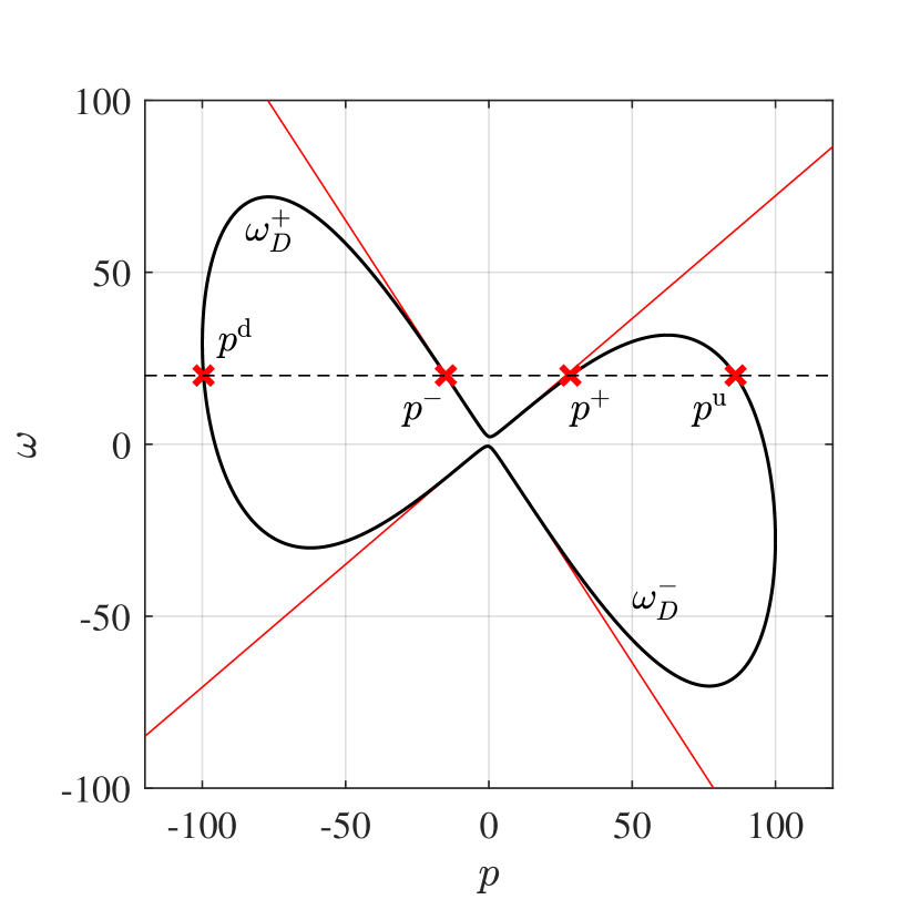
Figure 1: The branches of the dispersion relation $\omega_{D}^{\pm}$ in (25) for the parameters $m=5$, $C=2$ and $\Lambda=10^{-4}$ at the location $r=3.5$. The solid black curve corresponds to the weakly dispersive relation in (24) whereas the red curve is the shallow water limit with $\Lambda=0$. When the branches intersect with a line of constant $\omega$ (dashed black line) the dispersion relation has real solutions (red crosses).

Although (24) is only a good approximation of (23) for small $hk$, it manages to capture the qualitative features of the full dispersion relation (which also has four solutions) even for larger values of $hk$. That being said, it possesses certain non-physical features that one should take care to avoid. In particular:

1. At large $r$ there is a maximum frequency $\omega_{\mathrm{max}}=1/\sqrt{2\Lambda}$ above which none of the $p^{j}$ are real. Since the full dispersion relation has 4 propagating solutions at infinity, one should always work below this frequency.

2. Also at large $r$, the d mode is on the $\omega_{D}^{+}$ branch, compared to the full dispersion relation where it lies on $\omega_{D}^{-}$. To avoid this, the upper limit on $r$ should be selected so that the d mode is on the correct branch, e.g. Fig. 1.

3. When $r^{2}<\Lambda m^{2}$, the branches in (25) are complex for all $p$. Hence, one should work above this radius to ensure they are real for some $p$.

4. The extrema in the top left and bottom right of Fig. 1 are absent in the full dispersion relation. Thus, one needs to make sure that the $\omega=\mathrm{const}$ line does not cross these points as $r$ is varied, otherwise non-physical scattering will occur.

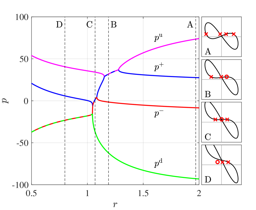
Figure 2: The four solutions of (24) for $\omega=17.7$, $m=2$, $C=10$ and $\Lambda=10^{-4}$. Only the real part of $p^{j}$ is shown. The curves are solid for $p^{j}\in\mathbb{R}$ and alternate in colour for $p^{j}\in\mathbb{C}$. The location of the $p^{j}$ on the branches of the dispersion relation is shown on the right at the locations indicated. In these panels, crosses indicate real $p\in\mathbb{R}$ whereas circles indicate $p\in\mathbb{C}$.

IV.5 The scattering matrix

The scattering matrix $\mathcal{M}$ is an $M\times M$ matrix which acts on the amplitudes defined in (22) at a point $r_{\mathrm{B}}$ and gives their value at another point $r_{\mathrm{A}}<r_{\mathrm{B}}$,

$$\mathbf{A}_{\mathrm{A}}=\mathcal{M}\mathbf{\mathbf{A}}_{\mathrm{B}},$$ (26)

where $\mathbf{A}_{\mathrm{A},\mathrm{B}}$ is an $M$ component column vector containing all the $A^{j}_{\mathrm{A},\mathrm{B}}=A^{j}(r_{\mathrm{A},\mathrm{B}})$ and $r_{\mathrm{A},\mathrm{B}}$ are the points in the system where one extracts the scattering amplitude. As a matter of convention, the amplitudes in $\mathbf{A}$ will always be ordered so that the mode with the largest $\mathrm{Re}[p^{j}]$ appears at the top and $\mathrm{Re}[p^{j}]$ decreases moving down the column vector.

The WKB solution in (21) encodes only the adiabatic change in a given mode as it moves from one point to another. In particular, if the WKB solution is known at a point $r_{b}$, then the solution at another point $r_{a}<r_{b}$ can be obtained by applying a shift factor,

$$\mathcal{F}^{j}_{ab}=\left|\frac{\mathcal{H}^{\prime}_{b}(p^{j})}{\mathcal{H}^{\prime}_{a}(p^{j})}\right|^{\frac{1}{2}}\exp\left(-i\int^{r_{b}}_{r_{a}}p^{j}dr\right).$$ (27)

provided the WKB solution is valid everywhere between $r_{a}$ and $r_{b}$ (note, these functions are scalars and not tensors; the lower indices indicate that the function is applied at $r_{b}$ and returns an object at $r_{a}$). Hence, if the WKB solutions are valid over the whole system, $\mathcal{M}$ will simply be a diagonal matrix containing the shift factors for the different modes. Such situations are usually of no interest since they contain no mode interactions and no scattering.

More interesting situations arise if there are points in the system where the WKB solution fails. At these locations, the different $p^{j}$ interact and the scattering matrix acquires off-diagonal terms that induce coupling between the modes. This interaction arises as a proximity (or intersection) of neighbouring paths in the $(r,p)$ phase space. An example of the phase space is given in Fig. 2. Consider now the region between the dashed lines labelled A and C. In this particular example, $|p^{j}|$ coincides for the $+$ and u modes over short distance around the line labelled B before the trajectories eventually move apart. For other parameters (in this example when lowering $\omega$), these trajectories may come very close to each other whilst never quite touching. Both of cases, one can estimate the mode coupling using the techniques about to be discussed. Since only neighbouring solutions can interact in this manner, it will suffice to consider only two mode interactions in the vicinity of special locations: these are the turning points and the saddle points of $\mathcal{H}$ (defined properly below). The different possible two mode interactions around these points are sketched in Fig. 3. Scattering events involves three or more modes can then be built up as a sequence of multiple two mode interactions. In the following, I will only state the $2\times 2$ matrices which relate the mode amplitudes at these points. The details of the derivation are left to Appendices B and C.

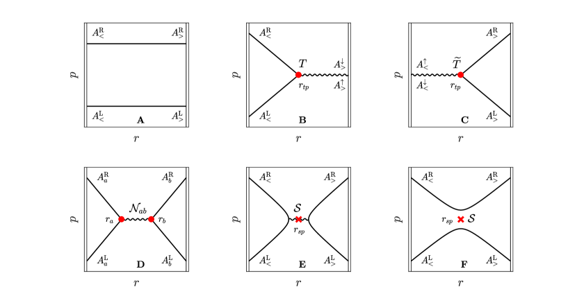
Figure 3: The different possible two mode interactions around turning points (red circles) and saddle points (red crosses). In panel A, there is no interaction. In panel B, there is a turning point where two evanescent modes at large $r$ are converted into propagating modes at small $r$. In panel C, the reverse happens. In panel D, there are two turning points which convert propagating modes into evanescent modes then back into propagating modes (this is a combination of the two previous cases). In panel E, the modes are converted at a saddle point with $b>0$. This method of conversion is preferable to that shown in panel D when the two turning points become close. In panel E, the modes are converted at a saddle point with $b<0$. Although there are no turning points, mode conversion occurs due to the proximity of the two solutions in the $(r,p)$ plane.

IV.5.1 Turning points

A turning point $r_{\mathit{tp}}$ is determined by the conditions,

$$\mathcal{H}_{\mathit{tp}}=0,\qquad\partial_{p}\mathcal{H}_{\mathit{tp}}=0,$$ (28)

which are to be solved at fixed $\omega$ and $m$ for the values $r_{\mathit{tp}}$ and $p_{\mathit{tp}}$, where subscript $\mathit{tp}$ denotes the value of a quantity on a turning point. These points are so named since, by Hamilton’s equations (16), they correspond to the locations where a classical particle comes to a halt and reverses it’s direction, i.e. $\dot{r}=0$. Using the expression for the Hamiltonian in (15), the conditions in (28) can be recast as equivalent conditions on the dispersion relation,

$$\omega={\omega_{D}^{\pm}}_{\mathit{tp}},\qquad\partial_{p}{\omega_{D}^{\pm}}_{\mathit{tp}}=0.$$ (29)

Hence the turning points are locations in the system where the extrema of $\omega_{D}^{\pm}$ are on-shell. On the extrema, two of the $p^{j}$ become equal and these modes will interact. Let two such modes be denoted $p^{\mathrm{L}}$ and $p^{\mathrm{R}}$ with $p^{\mathrm{L}}<p^{\mathrm{R}}$. By considering the form of the dispersion relation, e.g. in Fig. 1, it is clear that only neighbouring $p^{j}$ can interact in this manner.

The WKB solution clearly fails at $r_{\mathit{tp}}$, since the WKB amplitude (22) is inversely proportional to $\mathcal{H}^{\prime}$ which vanishes on the turning point. For $r<r_{\mathit{tp}}$ and $r>r_{\mathit{tp}}$, however, the WKB solution is still valid. To compare the WKB amplitudes in these regions, there is a standard procedure in which one finds an exact solution to the wave equation around the turning point and then matches this onto the WKB solutions. The details of this procedure can be found in Appendix B. The result is that the WKB modes mix with each other as the turning point is crossed. The mixing formulae can be expressed as a matrix that “transfers” the WKB solution across the turning point. If the interacting modes have $p^{j}(r<r_{\mathit{tp}})\in\mathbb{R}$ and $p^{j}(r>r_{\mathit{tp}})\in\mathbb{C}$, they are related by the $2\times 2$ transfer matrix $T$ according to,

$$\begin{pmatrix}A^{\mathrm{R}}_{<}\\ A^{\mathrm{L}}_{<}\end{pmatrix}=T\begin{pmatrix}A^{\downarrow}_{>}\\ A^{\uparrow}_{>}\end{pmatrix},\qquad T=e^{\frac{i\pi}{4}}\begin{pmatrix}1&-\tfrac{i}{2}\\ -i&\tfrac{1}{2}\end{pmatrix},$$ (30)

where the $A^{j}_{<}$ ($A^{j}_{>}$) are the WKB amplitudes (22) to the left (right) of $r_{\mathit{tp}}$ and the label $\uparrow$ ($\downarrow$) corresponds to the mode which grows (decays) in the direction of increasing $r$. In the mirror situation, where $p^{j}(r<r_{\mathit{tp}})\in\mathbb{C}$ and $p^{j}(r>r_{\mathit{tp}})\in\mathbb{R}$, the interacting modes are related by,

$$\begin{pmatrix}A^{\uparrow}_{<}\\ A^{\downarrow}_{<}\end{pmatrix}=\widetilde{T}\begin{pmatrix}A^{\mathrm{R}}_{>}\\ A^{\mathrm{L}}_{>}\end{pmatrix},\qquad\widetilde{T}=e^{\frac{i\pi}{4}}\begin{pmatrix}\tfrac{1}{2}&-\tfrac{i}{2}\\ -i&1\end{pmatrix},$$ (31)

The role of these two matrices is illustrated in panels B and C of Fig. 3. It is useful to define another matrix $\mathcal{N}_{ab}$ for scenarios where there are two turning points, which is formed by combining the previous two matrices with the WKB propagation matrix in between (see Appendix B for details). This matrix take the amplitudes of propagating modes at $r_{b}$ and returns the same at $r_{a}<r_{b}$, i.e.

$$\begin{pmatrix}A_{a}^{\mathrm{R}}\\ A_{a}^{\mathrm{L}}\end{pmatrix}=\mathcal{N}_{ab}\begin{pmatrix}A_{b}^{\mathrm{R}}\\ A_{b}^{\mathrm{L}}\end{pmatrix}.$$ (32)

with,

$$\begin{split}\mathcal{N}_{ab}=&\ \mathcal{F}_{ab}^{\downarrow}\begin{bmatrix}1+\tfrac{1}{4}f_{ab}^{2}&i\left(1-\tfrac{1}{4}f_{ab}^{2}\right)\\ -i\left(1-\tfrac{1}{4}f_{ab}^{2}\right)&1+\tfrac{1}{4}f_{ab}^{2}\end{bmatrix},\\ f_{ab}=&\ \exp\left(-\int^{r_{b}}_{r_{a}}\mathrm{Im}[p^{\downarrow}]dr\right),\end{split}$$ (33)

The role of $\mathcal{N}_{ab}$ is illustrated in panel D of Fig. 3. Note, it is also possible to define a similar matrix relating evanescent modes in this manner, which applies when there are bound states Patrick et al. (2018a). I will not pause to do this here, since the model example in (7) is a monotonically decreasing function of $r$ and therefore does not contain bound states.

IV.5.2 Saddle points

A saddle point $r_{\mathit{sp}}$ is determined by the conditions,

$$\partial_{r}\mathcal{H}_{\mathit{sp}}=0,\qquad\partial_{p}\mathcal{H}_{\mathit{sp}}=0.$$ (34)

which are to be solved at fixed $\omega$ and $m$ for the values $r_{\mathit{sp}}$ and $p_{\mathit{sp}}$, where subscript $\mathit{sp}$ denotes the value of a quantity on the saddle point. The first thing to notice is that, unlike turning points, these locations are not in necessarily on-shell. Therefore, in general, $\mathcal{H}_{\mathit{sp}}\neq 0$ (apart from in special cases to be discussed later).

Saddle points are concerned with propagating modes which approach $r_{\mathit{sp}}$ from both sides, see Fig. 3. Depending on the properties of the saddle point, these modes can either bounce off $r_{\mathit{sp}}$ (panel E) or pass straight through it (panel F). The matrix connecting the mode amplitudes is again found by searching for an exact solution to the wave equation around $r_{\mathit{sp}}$, and matching this onto the WKB solutions (details in Appendix C). The connection formula is Torres (2020),

$$\begin{pmatrix}A_{<}^{\mathrm{R}}\\ A_{<}^{\mathrm{L}}\end{pmatrix}=\mathcal{S}\begin{pmatrix}A_{>}^{\mathrm{R}}\\ A_{>}^{\mathrm{L}}\end{pmatrix},$$ (35)

with,

$$\begin{split}\mathcal{S}=&\ \tau^{-1}\begin{bmatrix}\beta\alpha^{2}&i\\ -i&\beta^{*}\alpha^{-2}\end{bmatrix},\qquad\tau=e^{-\pi b},\\ \alpha=&\ 2^{\frac{ib}{2}}e^{-\frac{i\pi}{8}},\qquad\beta=\frac{\sqrt{2\pi i\tau}}{\Gamma(\tfrac{1}{2}+ib)},\end{split}$$ (36)

where $\Gamma(z)$ is the Gamma function and the parameter $b$ determines the properties of the saddle point,

$$b=\frac{\mathrm{sgn}(\mathcal{H}^{\prime\prime}_{\mathit{sp}})\mathcal{H}_{\mathit{sp}}}{\sqrt{-\mu_{+}\mu_{-}}}.$$ (37)

The $\mu_{+}\mu_{-}$ term (explained in Appendix C) is always real and negative due to the saddle structure, so the sign of $b$ is determined by the numerator.

The situation in panel E of Fig. 3 corresponds to $b>0$. This case is similar to that shown in panel D, since it also contains turning points where propagating modes become evanescent. However, once the distance between the turning points becomes small, the WKB solution ceases to be a good approximation in between and the conversion matrix in panel D will fail. In particular, the WKB solution is only accurate if the wavelength is shorter than the distance characterising the change in the background. Hence, an appropriate condition for choosing which matrix to apply is the following,

$$\begin{split}p_{\mathit{sp}}(r_{b}-r_{a})>1&\quad\to\quad\mathcal{N}_{ab}\\ p_{\mathit{sp}}(r_{b}-r_{a})<1&\quad\to\quad\mathcal{S}\\ \end{split}$$ (38)

The situation in panel F of Fig. 3 corresponds to $b<0$. Technically, the WKB solution is valid everywhere in this case and, as such, the mode coupling results from the fact WKB is not an exact solution. Indeed, one can see that the mode coupling is exponentially suppressed in this case as expected due to the presence of exponentials in (36). For large negative $b$, the matrix $\mathcal{S}$ asymptotically approaches the identity matrix and one effectively recovers the scattering scenario in panel A.

IV.5.3 Computing $\mathcal{M}$

With these tools at our disposal, we are well-poised to tackle a computation of the full scattering matrix for generic dispersion relations of the form (9). The method proceeds as follows,

1. Solve $\mathcal{H}=0$ for the different $p^{j}$ and plot the solutions in the $(r,p)$ plane (e.g. Fig. 2).

2. Locate the turning points and saddle points using (28) and (34), then identify the dominant two mode interactions of the type shown in Fig. 3.

3. Each non-interacting mode is evolved adiabatically according to the shift factor in (27).

4. At each interaction, multiply the mode amplitudes by the relevant matrix $T,\widetilde{T},\mathcal{N}_{ab}$ or $\mathcal{S}$.

As an illustrative example, consider the case depicted in Fig. 2. In this scenario, there are 5 turning points which I will call $r_{1,2,3,4,5}$ from left to right. Let us compare the mode amplitudes at the locations given by the dashed lines labelled A and D,

$$\begin{pmatrix}A_{\mathrm{D}}^{\mathrm{u}}\\ A_{\mathrm{D}}^{+}\\ A_{\mathrm{D}}^{\uparrow}\\ A_{\mathrm{D}}^{\downarrow}\\ \end{pmatrix}=\mathcal{M}\begin{pmatrix}A_{\mathrm{A}}^{\mathrm{u}}\\ A_{\mathrm{A}}^{+}\\ A_{\mathrm{A}}^{-}\\ A_{\mathrm{A}}^{\mathrm{d}}\\ \end{pmatrix}.$$ (39)

The scattering matrix is,

$$\begin{split}\mathcal{M}=\begin{pmatrix}\mathcal{F}^{\mathrm{u}}_{\mathrm{D}1}&&&\\ &\mathcal{F}^{+}_{\mathrm{D}1}&&\\ &&\mathcal{F}^{\uparrow}_{\mathrm{D}1}&\\ &&&\mathcal{F}^{\downarrow}_{\mathrm{D}1}\end{pmatrix}\begin{pmatrix}1&&\\ &1&\\ &&\widetilde{T}\end{pmatrix}\mathcal{J}_{12}\begin{pmatrix}\mathcal{F}^{\mathrm{u}}_{23}&&\\ &\mathcal{N}_{23}&&\\ &&\mathcal{F}^{\mathrm{d}}_{23}\end{pmatrix}\mathcal{J}_{34}\begin{pmatrix}\mathcal{N}_{45}&&\\ &\mathcal{F}^{-}_{45}&&\\ &&\mathcal{F}^{\mathrm{d}}_{45}\end{pmatrix}\mathcal{J}_{5\mathrm{A}}\end{split}$$ (40)

where $\mathcal{J}_{ab}$ is a diagonal matrix, containing the shift factors, which translates propagating modes from $r_{b}$ to $r_{a}$. Notice that all that was necessary to write down (40) was to inspect the $(r,p)$ phase space in Fig. 2 and compare with the two mode interactions in Fig. 3. The precise locations of the turning/saddle points can then be obtained by solving the conditions in (28) and (34). If a single expression for $\mathcal{M}$ is required, it is straight forward to evaluate (40) computationally (performing the matrix multiplications by hand gets rather tedious after a while). In what follows, however, it turns out that the form of $\mathcal{M}$ as written in (40) will be more useful, since this allows one to isolate the relevant scattering channels.

V Application to gravity waves

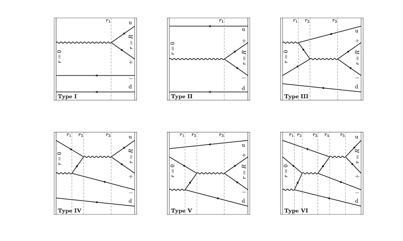
Figure 4: The phase space diagrams representing the different allowed scattering processes experienced by weakly dispersive gravity waves around a DBT. The type of scattering that occurs depends on the wave and background parameters, as shown in Fig. 5. Notice how these diagrams are constructed by stitching together the diagrams for the two mode interactions around turning points in Fig. 3.

In this section, I will apply the formalism established in the previous section to fully characterise the scattering of weakly dispersive gravity waves around a DBT. In other words, I will detail all the possible interactions (involving turning points and saddle points) allowed by the dispersion relation in (24). The crucial step will be to identify the characteristic frequencies which divide up the parameter space into regions where different scattering processes occur. To this end, I will first introduce the key frequencies before illustrating the different scattering types.

V.1 Light-ring frequencies

The first pair of important frequencies are the co- and counter-rotating light-ring frequencies $\omega_{\mathit{lr}}^{\pm}$, where the $\pm$ corresponds to the sign of $m$. In the non-dispersive case (i.e. $\Lambda=0$) these are analogous to null geodesics in black hole physics which orbit the system on closed paths Cardoso et al. (2009). For generic dispersion relations, they correspond to the critical points of the effective Hamiltonian Torres et al. (2018b). In terms of the discussion of the previous section, these locations have a simple interpretation: they are the locations where a saddle point of $\mathcal{H}$ is also a turning point. Hence, the light-ring conditions are,

$$\mathcal{H}_{\mathit{lr}}=0,\qquad\partial_{r}\mathcal{H}_{\mathit{lr}}=0,\qquad\partial_{p}\mathcal{H}_{\mathit{lr}}=0,$$ (41)

which are solved at fixed $m$ for the light-ring $r_{\mathit{lr}}$, as well as the frequency $\omega_{\mathit{lr}}$ and momentum $p_{\mathit{lr}}$ of a mode on the light-ring. There is also a simple interpretation for these frequencies in the particle picture; they correspond to the energy required for a particle of given angular momentum to orbit the system indefinitely on a closed trajectory.

Note that in Torres et al. (2018b), simple analytic expressions were provided for the light-rings of gravity waves around a DBT in the shallow and deep water regimes. In the present case, however, it is simpler to solve (41) numerically.

V.2 Critical frequencies

The second pair of important frequencies are the upper and lower critical frequencies, $\omega_{c}$ and $\omega_{\star}$ respectively. They are given by the conditions,

$$\mathcal{H}_{c,\star}=0,\qquad\partial_{p}\mathcal{H}_{c,\star}=0,\qquad\partial_{p}^{2}\mathcal{H}_{c,\star}=0,$$ (42)

which are again solved for a $(r,p,\omega)$ triplet. Hence, these points correspond to the inflection points of the effective Hamiltonian in the $p$ direction. The importance of these frequencies can be understood as follows.

From (15), an inflection point of the Hamiltonian is also an inflection point of one of the branches of the dispersion relation. Starting at large $r$, there will be four real propagating solutions and three extrema on both the upper and lower branches of the dispersion relation (see e.g. Fig. 1). As $r$ is decreased, the branches will rotate clockwise due to the linear term in $p$ in (25), causing the two extrema on the right of the upper branch to approach one another, and the same for the two extrema on the left of the lower branch. At a critical value of $r$, the extrema meet to become an inflection point. On the upper branch, the inflection point is given by $(p_{c},\omega_{c})$ and on the lower branch at $(p_{\star},\omega_{\star})$. Due to the symmetry of the dispersion relation (24), the following relations are satisfied: $r_{c}=r_{\star}$, $p_{c}=-p_{\star}$, $\omega_{c}(m<0)=-\omega_{\star}(m>0)$ and $\omega_{\star}(m<0)=-\omega_{c}(m>0)$.

Inside of the inflection point, there will only be one propagating mode on each branch of the dispersion relation. The crucial observation comes from noting that $\omega_{c}$ and $\omega_{\star}$ dictate which of the four modes are propagating and which are evanescent. On the upper branch, the u mode will be the real one for $\omega<\omega_{c}$, whereas above $\omega_{c}$, the $-$ mode is the real one. For the lower branch, the d mode will be real above $\omega_{\star}$ and below $\omega_{\star}$ the $+$ mode is real. These observations are summarised in the parameter space plot of Fig. 5 (discussed further in the next section). Note that $\omega_{\star}$ plays no role for positive frequency modes with $m<0$. This is simply because $\omega_{\star}$ concerns the lower branch of the dispersion relation, which for $m<0$ gets pushed to increasingly negative frequencies as $r$ is decreased due to the $mC/r^{2}$ term in (25).

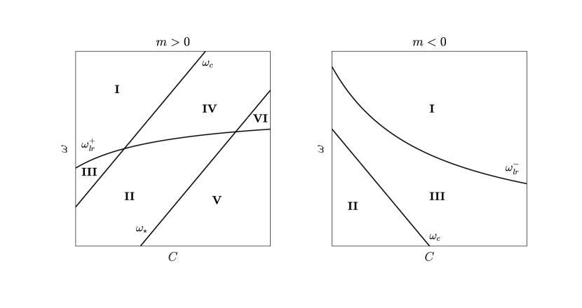
Figure 5: A schematic illustration of the parameter space for weakly dispersive gravity waves scattering with the DBT (the bottom-left corner is the point $\omega=0$, $C=0$). The light-ring and critical frequencies delineate the regions where different scattering processes occur. The precise form of these curves depends on the value of $m$ and $\Lambda$. However, the intersections between the curves is qualitatively as shown provided $m$ and $\Lambda$ are not chosen too large (discussed in Section IV.4). There are two distinct behaviours depending on the sign of $m$. For $m=0$, the type I process occurs everywhere in the parameter space.

V.3 Scattering processes

With these frequencies in hand, we are in a position to look at the allowed scattering processes that occur in (24). For the four restrictions laid out in Section IV.4, there are three in-going modes and one out-going mode at large $r$ (say $r=R$), and two in-going modes and two evanescent modes approaching $r=0$. Consequently, there must always be an odd number of turning points, the relative locations of which determine the type of scattering that occurs. The different possibilities can be grouped into 6 categories, whose phase space diagrams are illustrated in Fig. 4. We have already seen an example of such a diagram in Fig. 2, which corresponds to a type VI scattering event. The procedure of writing down the scattering matrix for the other five types proceeds analogously to that outlined in equation (40).

The type of scattering depends in general on the wave parameters $\omega$ and $m$, as well as the flow parameters $C$ and $\Lambda$. The light-ring and critical frequencies divide up the parameter space into regions where the different scattering types occur. However, the restrictions in Section IV.4 mean that the values of $\Lambda$ and $m$ cannot be too large, otherwise non-physical behaviour occurs at small $r$. When this non-physical behaviour is avoided, a slice of parameter space through the $\omega,C$ plane looks as illustrated in Fig. 5. This diagram clearly indicates that by moving through parameter space, one can transition between the different scattering possibilities. The two critical frequencies involve a discontinuous change between the character of the modes at small $r$ (i.e. propagating or evanescent) and hence appear as sharp boundaries in the parameter space. By contrast, the transition across the light-ring frequency is smoothed over as the interacting modes gradually couple/decouple, depending on the direction of crossing. The smoothed transition can be incorporated into the scattering matrix using the saddle point formula in (35). This procedure, which involves replacing the relevant turning point interactions in Fig. 4 with saddle point interactions, is illustrated in Fig. 6.

Using the diagrams in Fig. 4, it is also possible to identify the generalisation of the black hole horizon to the dispersive case. In shallow water, the horizon is a one-way membrane which lets the in-coming long-wavelength mode through but blocks the out-going one from escaping. For scattering types I and III, one can see that the horizon is replaced by the turning point $r_{1}$ where an in-coming u mode is converted into an out-going $+$ mode, whilst the $-$ and d modes pass through unimpeded. For types V and VI, the same thing happens except the roles of these pairs are exchanged. However, for types II and IV, dispersion completely blocks the long wavelength modes from propagating into the centre. In this sense, there is no natural generalisation of the horizon in the frequency range $\omega_{\star}<\omega<\omega_{c}$.

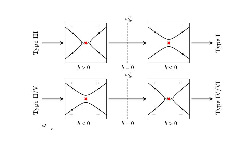
Figure 6: The interaction between modes which couple/decouple at the light-ring frequency is better described using the saddle point interaction. The figure illustrates how to replace the relevant interactions in Fig. 4 when this occurs. The frequency increases from left to right. The saddle point is indicated by a red cross.

V.4 Quasinormal modes

I will now demonstrate how to apply this formalism by using it to compute the characteristic modes of the system, or the quasinormal modes (QNMs).

An excited closed system will vibrate in it’s normal modes. These are solutions to the equations of motion which satisfy a particular set of boundary conditions, which usually involve either the field or it’s first spatial derivative going to zero on the boundary. Common examples include the frequencies of a plucked guitar string and the energy levels of a particle in a box. Similarly, an excited open system will vibrate in it’s quasinormal modes. These are dissipative solutions to the equation of motion which decay in time as they transfer energy out of the system. Consequently, their frequency spectrum is complex,

$$\omega_{\mathrm{QN}}=\mathrm{Re}[\omega_{\mathrm{QN}}]+i\mathrm{Im}[\omega_{\mathrm{QN}}],$$ (43)

where the real part gives the oscillation frequency and the imaginary part determines the decay rate. Mathematically, the QNM frequencies can be found by imposing purely transmissive boundary conditions on the system’s open boundary. In other words, waves can leave the system but none may come back in. I begin the discussion by detailing the implementation of these conditions.

V.4.1 Boundary conditions

For non-dispersive waves around a DBT, the QNM boundary conditions are that the wave is purely in-going on the horizon and purely out-going at infinity Berti et al. (2004). Hence, the boundary conditions consist in setting the amplitudes of the out-going mode on the horizon and the in-going mode at infinity to zero. Since the non-dispersive system is second order in spatial derivatives, these two boundary conditions provide all the necessary information to uniquely determine the eigen-frequencies.

In the dispersive case, the boundary conditions will be complicated by the fact that there are extra modes in the system. Specifically, the weakly dispersive system in (24) is fourth order in spatial derivatives, hence, one must supply a total of four boundary conditions to uniquely determine the eigen-frequencies. Each of the processes in Fig. 4 have three in-going modes at $r=R$, hence, the first three boundary conditions consist in setting these to zero. The remaining boundary condition is fixed by realising that one of the evanescent solutions diverges approaching $r=0$, therefore it’s amplitude should also be set to zero. In summary, setting,

$$A_{R}^{\mathrm{u}}=A_{R}^{-}=A_{R}^{\mathrm{d}}=A_{0}^{\downarrow}=0,$$ (44)

uniquely determines the eigenmodes of the weakly dispersive system, which are defined to be the quasinormal modes. Since the solution to the wave equation is determined upto an overall constant, one of the remaining amplitudes can be set to one. For the QNMs, this is conventionally chosen to be the out-going mode at infinity, i.e.

$$A_{R}^{+}=1.$$ (45)

V.4.2 The QNM condition

Since the QNMs have a particular oscillation frequency, they will correspond to a particular type of scattering. With the correct boundary conditions identified, we can systematically begin applying them to each of the scattering possibilities in Fig. 4 to determine which of them contain quasinormal modes. The type I and II processes can be immediately ruled out as candidates since implementing (44) trivially fixes all the remaining amplitudes to be zero. The other four scenarios require more care to analyse, hence, I address them one-by-one. The general QNM condition will be presented at the end of this section in equation (53).

In type III scattering, the d mode decouples from the rest and thus, one can immediately set $A_{0}^{\mathrm{d}}=0$. Furthermore, the u mode is completely reflected at $r_{1}$, thus by (44), one must also have $A_{0}^{\uparrow}=0$. Thus, the problem is reduced to considering the scattering that occurs between the turning points $r_{2}$ and $r_{3}$. It only remains to choose whether to implement the turning point or saddle point conversion matrix at this interaction, i.e. $\mathcal{N}_{23}$ or $\mathcal{S}$. It turns out that for the QNMs, the turning points $r_{2}$ and $r_{3}$ are close together and thus, the saddle point interaction is the appropriate choice (this is also known in the non-dispersive case Berti et al. (2009)). Applying the boundary conditions gives,

$$\begin{pmatrix}0\\ A^{-}_{<}\end{pmatrix}=\mathcal{S}\begin{pmatrix}A^{+}_{>}\\ 0\end{pmatrix}\quad\Rightarrow\quad\frac{\beta\alpha^{2}}{\tau}\mathcal{F}^{+}_{>R}=0,$$ (46)

where $\mathcal{F}^{+}_{>R}$ is the shift factor for the $+$ mode from $r=R$ up to the right of the saddle point. Recalling the definition of $\beta$ in (36), one can see that this condition is satisfied for the poles of the Gamma function, i.e. when it’s argument is equal to $-n$ where $n$ spans the natural numbers starting from 0. Thus, in the type III diagram, QNMs exist for,

$$n+\tfrac{1}{2}+ib=0,$$ (47)

with $b$ given in (37).

The analysis for type IV scattering proceeds in a similar fashion. Again, one finds that the problem can be reduced to considering the interaction around the turning points $r_{2}$ and $r_{3}$, which using the saddle point formula gives,

$$\begin{pmatrix}A^{\mathrm{u}}_{<}\\ 0\end{pmatrix}=\mathcal{S}\begin{pmatrix}0\\ A^{+}_{>}\end{pmatrix}\quad\Rightarrow\quad\frac{\beta^{*}\alpha^{-2}}{\tau}\mathcal{F}^{+}_{>R}=0.$$ (48)

Consequently, the QNM condition in the type IV diagram is,

$$n+\tfrac{1}{2}-ib=0,$$ (49)

which differs from the type III condition in (47) only by a minus sign.

The type V process differs from the previous two cases due to the way the $+$ mode approaches the origin. The boundary conditions immediately give $A_{0}^{\uparrow}=A_{0}^{\mathrm{u}}=0$. The turning points $r_{2}$ and $r_{3}$ correspond to a transfer from the upper branch to the lower branch of the dispersion relation. Since this gap increases with $m$ (and the present method improves for large $m$) the turning points will be far apart and the interaction is well represented by the $\mathcal{N}_{23}$ matrix,

$$\begin{pmatrix}A^{+}_{2}\\ 0\end{pmatrix}=\mathcal{N}_{23}\begin{pmatrix}A^{+}_{3}\\ 0\end{pmatrix}\quad\Rightarrow\quad-i(1-\tfrac{1}{4}f_{23})\mathcal{F}^{+}_{>R}=0.$$ (50)

This condition is nowhere satisfied for the frequency range in which type V scattering occurs. Hence, type V scattering contains no QNMs.

Finally, the type VI process contains interactions between all four modes. The boundary conditions impose that $A_{0}^{\uparrow}=0$, thus the interaction between $r_{2}$ and $r_{3}$ is described by the same matrix equation as in (50). Using the saddle point conversion matrix at the next interaction along gives,

$$\begin{pmatrix}A^{\mathrm{u}}_{<}\\ A^{+}_{<}\end{pmatrix}=\mathcal{S}\begin{pmatrix}0\\ A^{+}_{>}\end{pmatrix}.$$ (51)

Using the shift factor to connect the amplitudes between $r_{2}$ and the left of the saddle point, then implementing the boundary conditions at $r=R$, results in,

$$-i(1-\tfrac{1}{4}f_{23})\frac{\beta^{*}\alpha^{-2}}{\tau}\mathcal{F}^{+}_{3<}\mathcal{F}^{+}_{>R}=0,$$ (52)

which is simply a combination of the conditions in (48) and (50). Since the bracketed factor is nowhere vanishing in the allowed frequency range, the QNMs are again determined by the poles of the Gamma function, which gives the same condition as in (48).

We now have two different QNM conditions: (47) in type III scattering and (49) for types IV and VI. These can be unified into a single condition by noticing the following. The definition of $b$ in (37) contains a factor of $\mathrm{sgn}(\mathcal{H}^{\prime\prime}_{\mathit{sp}})$ which is positive in type III and negative in types IV and VI (more on this in the next section). This acts to eliminate the sign difference between (47) and (49). Thus, the single condition that gives the QNM frequencies (within the WKB approximation) is,

$$\frac{\mathcal{H}_{\mathit{sp}}}{\sqrt{-\mu_{+}\mu_{-}}}=i\left(n+\tfrac{1}{2}\right).$$ (53)

This is the familiar QNM condition from the non-dispersive case Berti et al. (2009), albeit from the viewpoint of the Hamiltonian rather than the effective potential. The present analysis reveals that the condition also holds in dispersive systems. The number $n$ is called the overtone number and essentially classifies the different QNMs according to their lifetime. Usually, the fundamental mode with $n=0$ is the one of most interest since it is the longest lived. In practice, (53) can be solved at fixed $n,m,C$ and $\Lambda$ using a standard root finding algorithm (I used Matlab’s inbuilt fsolve function for it’s robustness). In Fig. 7, the dependence of $\omega_{\mathrm{QN}}$ on $C$ is illustrated for $|m|=5$ for different values of $\Lambda$, and Fig. 8 shows the variation with $\Lambda$ for various $C$ values. Both plots demonstrate that the counter-rotating modes are insensitive to changes in the dispersive parameter, whereas the co-rotating modes depend strongly on $\Lambda$ above a critical $C$ dependent value. This observation is explained in the next section.

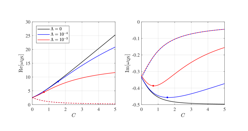
Figure 7: The QNM spectrum for $m=5$ (solid lines) and $m=-5$ (dashed lines) for different values of the dispersive parameter. The counter-rotating rotating modes show little to no variation in the spectrum when increasing dispersion (at large $C$, the three curves are basically overlapping). Conversely, the co-rotating modes are heavily dependent on $\Lambda$. This variation in the spectrum corresponds to a change in the modes involved in the interaction. At the dots on the red and blue curves, $\mathcal{H}^{\prime\prime}_{\mathit{tp}}=0$ on the light-ring. To the left of the dots, the QNMs involve the $+$ and $-$ modes whereas to the right, they involve the u and $+$ modes.

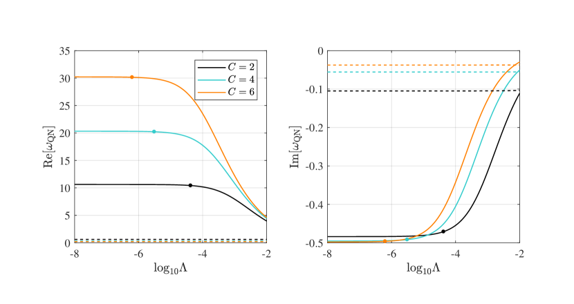
Figure 8: The QNM spectrum for $m=5$ (solid lines) and $m=-5$ (dashed lines) for different values of the rotation parameter. The counter-rotating rotating modes show little to no dependence on the dispersive parameter. The same is also true for the co-rotating modes when dispersion is weak. However, there is a critical point where $\mathcal{H}^{\prime\prime}_{\mathit{tp}}=0$ at the light-ring (shown as a dot) and past this point, the size of both the real and imaginary part of $\omega_{\mathrm{QN}}$ begins to decrease with increasing $\Lambda$. This change in behaviour corresponds to a change in the modes involved in the interaction: to the left of the points on the curves, the $+$ and $-$ modes are involved whereas to the right, it is the u and $+$ modes which interact.

V.4.3 Interpretation

It is well-known in black hole physics that real part of the QNM frequency is well approximated by the light-ring frequency Cardoso et al. (2009). The reason for this is that the ratio $\mathrm{Re}[\omega_{\mathrm{QN}}]/\mathrm{Im}[\omega_{\mathrm{QN}}]$ grows with increasing $|m|$, hence, the imaginary part can be treated as a small correction to the real part for large $|m|$. At leading order, the QNM condition (53) decouples into two equations,

$$\mathcal{H}_{\mathit{sp}}(\mathrm{Re}[\omega_{\mathrm{QN}}])\approx 0,\qquad\mathrm{Im}[\omega_{\mathrm{QN}}]\approx i(n+\tfrac{1}{2})\frac{\sqrt{-\mu_{+}\mu_{-}}}{\partial_{\omega}\mathcal{H}_{\mathit{sp}}},$$ (54)

where the right-hand side of the second equation is evaluated at $\mathrm{Re}[\omega_{\mathrm{QN}}]$. The first equation is simply the condition for the light-ring mode in (41), hence,

$$\mathrm{Re}[\omega_{\mathrm{QN}}]\approx\omega^{\pm}_{\mathit{lr}},$$ (55)

where the $+$ or $-$ sign is taken depending on the sign of $m$. The expression for the imaginary part in (54) was also found in Torres et al. (2018b) by considering the divergence of neighbouring rays near the light-ring. Within this approximation, an intuitive picture of the QNMs in terms of an effective potential barrier emerges, as we shall now see. This picture leads to a natural explanation of why the co-rotating QNMs depend strongly on $\Lambda$ whereas the counter-rotating modes do not.

The key step in this argument will be to identify how the relevant two modes interact around the light-ring. In fact, since the light-ring is simply a turning point which is also a saddle point, one can be even more general and consider the interaction of two modes around a turning point at each location in $r$. To do this, consider a local expansion of the Hamiltonian around a turning point. This amounts to expanding the branches of the dispersion relation around the extrema. Since the light-rings are concerned with the upper branch, it will suffice to consider an expansion of $\omega_{D}^{+}$. The turning point conditions (28) give the location of the extremum $p_{\mathit{tp}}=p_{\mathit{tp}}(r)$ and the value of the branch there $\omega^{+}_{\mathit{tp}}=\omega_{D}^{+}(r,p_{\mathit{tp}})$. Locally, the Hamiltonian is,

$$\mathcal{H}=\partial_{\omega}\mathcal{H}_{\mathit{tp}}(\omega-\omega^{+}_{\mathit{tp}})+\tfrac{1}{2}\mathcal{H}^{\prime\prime}_{\mathit{tp}}(p-p_{\mathit{tp}})^{2}.$$ (56)

On the upper branch, one has $-\partial_{\omega}\mathcal{H}_{\mathit{tp}}=\Omega_{\mathit{tp}}>0$. On-shell solutions then satisfy,

$$\omega=\frac{1}{2}\frac{\mathcal{H}^{\prime\prime}_{\mathit{tp}}}{\Omega_{\mathit{tp}}}P^{2}+\omega^{+}_{\mathit{tp}},$$ (57)

where $P=p-p_{\mathit{tp}}$ is the local wavevector. This is precisely of the form of a classical energy relation for a particle with energy $\omega$ moving through a potential $\omega^{+}_{\mathit{tp}}(r)$. This is to be expected since (57) has been derived under the assumption that $P$ is small. Points where $\partial_{r}\omega^{+}_{\mathit{tp}}=0$ correspond precisely to the light-ring. Note also that the kinetic energy term in (57) can be either positive or negative due to the presence of $\mathcal{H}^{\prime\prime}_{\mathit{tp}}$.

The momentum of the particle is given by,

$$P=\pm\sqrt{\frac{2\Omega_{\mathit{tp}}(\omega-\omega^{+}_{\mathit{tp}})}{\mathcal{H}^{\prime\prime}_{\mathit{tp}}}},$$ (58)

which distinguishes two possibilities depending on the sign of $\mathcal{H}^{\prime\prime}_{\mathit{tp}}$. In both of these cases, the extremum of $\omega^{+}_{\mathit{tp}}(r)$ plays a crucial role.

1. For $\mathcal{H}^{\prime\prime}_{\mathit{tp}}>0$, the particle classically propagates for $\omega>\omega^{+}_{\mathit{tp}}$, i.e. above the potential barrier. If $\omega^{+}_{\mathit{tp}}$ has a local maximum, the energy to be at rest at this point represents the minimum energy required for the particle to classically cross from one side of the barrier to the other.

2. For $\mathcal{H}^{\prime\prime}_{\mathit{tp}}<0$, the particle classically propagates for $\omega<\omega^{+}_{\mathit{tp}}$, i.e. below the potential barrier. If $\omega^{+}_{\mathit{tp}}$ has a local minimum, the energy to be at rest there represents the maximum energy the particle can have whilst classically propagating from one side to the other.

In the first case the light-ring frequencies are energy minima whereas in the second case they are energy maxima. Ultimately this is due to the fact that in case 1, the light-ring involves the $+$ and $-$ modes, which interact at a minimum (${\omega_{D}^{+}}^{\prime\prime}>0$) of the dispersion relation whereas in case 2, the light-ring involves the u and $+$ modes which interact at a maximum (${\omega_{D}^{+}}^{\prime\prime}<0$) of the dispersion relation.

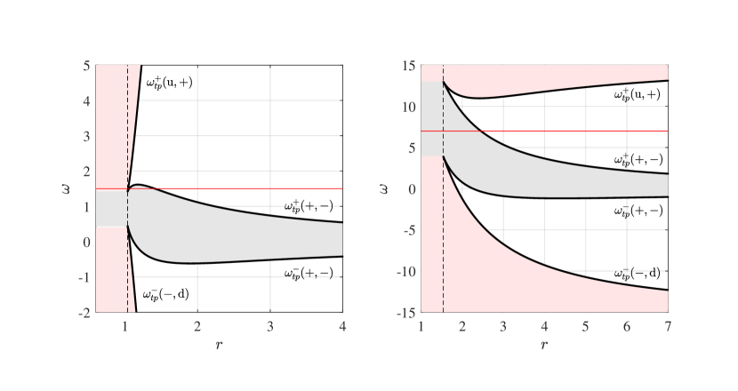
Figure 9: The dependence of the extrema of the dispersion relation (black curves) on $r$. The extrema merge at the inflection point (dashed black line). In the grey region, the $+$ and $-$ modes are evanescent whereas in the upper (lower) pink region, the u and $+$ ($-$ and d) modes are evanescent. For fixed frequency, these curves determine the locations where different modes interact. The curves which mix the $+$ and $-$ modes have $\mathcal{H}^{\prime\prime}_{\mathit{tp}}>0$ whereas the other two have $\mathcal{H}^{\prime\prime}_{\mathit{tp}}<0$. On the left, the parameters are $m=2$, $C=0.5$, $\Lambda=10^{-4}$. In this case, the radial extremum for $\omega>0$ modes is a maximum on the $\omega_{\mathit{tp}}^{+}(+,-)$ curve. An example frequency is illustrated (red line) which corresponds to type III scattering. On the right, the parameters are $m=10$, $C=2$, $\Lambda=10^{-3}$. In this case, the radial extremum for $\omega>0$ modes is a minimum on the $\omega_{\mathit{tp}}^{+}(+,\mathrm{u})$ curve. The example frequency (red line) corresponds to type II scattering. Note that (24) is invariant under the exchange $\omega\to-\omega$ and $m\to-m$. Hence, these diagrams can also be used to describe $m<0$ modes if one makes the changes $\omega_{\mathit{tp}}^{+}\to-\omega_{\mathit{tp}}^{-}$ and $\omega_{\mathit{tp}}^{-}\to-\omega_{\mathit{tp}}^{+}$. In this case, the extremum is always a maximum on $\omega_{\mathit{tp}}^{+}(+,-)$ and thus, the behaviour of the counter-rotating light-ring is always the same.

Using (58), the $\omega^{+}_{\mathit{tp}}$ may be interpreted as the minimum/maximum energy for which a pair of modes may propagate at a given radius. The same can be said for the $\omega^{-}_{\mathit{tp}}$ curves on the lower branch of the dispersion relation. There are six such curves in total, corresponding to the six extrema of 25 which can be clearly seen in Fig. 1. However, only four of these are physical (the two on the right of the upper branch and the left of the lower branch) with the remaining two being non-physical artefacts of the weakly dispersive approximation. Let the four physical extrema be denoted $\omega^{+}_{\mathit{tp}}(+,-)$, $\omega^{+}_{\mathit{tp}}(u,+)$, $\omega^{-}_{\mathit{tp}}(+,-)$ and $\omega^{+}_{\mathit{tp}}(-,\mathrm{d})$, where the brackets indicate which modes are interacting. These curves are illustrated in Fig. 9 for two different cases. The shaded regions represent parts of the system where the propagation of certain modes is forbidden. If the extremum ($\partial_{r}\omega_{\mathit{tp}}=0$) lies on a curve with $\mathcal{H}^{\prime\prime}_{\mathit{tp}}>0$, it is a local maximum, whereas on curves with $\mathcal{H}^{\prime\prime}_{\mathit{tp}}<0$ it is a local minimum. This behaviour corresponds exactly to that discussed in the two cases above.

The switch over from one case to another occurs when $\mathcal{H}^{\prime\prime}_{\mathit{tp}}=0$, which is none other than the condition for the critical frequency in (42). Hence, the light-ring frequency changes from an energy minimum to an energy maximum when it intersects the upper critical frequency in the parameter space. In Fig. 5, this happens for a particular value of $C$ (say $C_{\mathit{int}}$). The dependence of $C_{\mathit{int}}$ on $\Lambda$ is shown in Fig. 10 for the first five $m$’s. This shows that the value of $C_{\mathit{int}}$ decreases with increasing $m$ and $\Lambda$. Note that $C_{\mathit{int}}<0$ corresponds to a structurally different parameter space than that shown in Fig. 5. This only happens when $m$ and $\Lambda$ are too large, which would violate the restrictions on weakly dispersive system outlined in Section IV.4. Hence, only $C_{\mathit{int}}>0$ is of interest and the parameter space always looks like Fig. 5.

In Fig. 7, the location of $C_{\mathit{int}}$ is shown as a point on the $m>0$ curves. At this point, there is a clear change in the behaviour of the mode; specifically, there is a slower increase in the size of $\mathrm{Re}[\omega_{\mathrm{QN}}]$ with $C$ and the size of the $\mathrm{Im}[\omega_{\mathrm{QN}}]$ decreases. In Fig. 8, the value of $\Lambda$ for which $C_{\mathit{int}}$ equals the value displayed is also plotted as a point. To the right of this point, the size of both the real and imaginary parts of $\omega_{\mathrm{QN}}$ decreases with increasing $\Lambda$. Since $\omega_{c}$ intersects nowhere with $\omega^{-}_{\mathit{lr}}$ for $\omega>0$, the counter-rotating modes are not subject to the same change in behaviour, thereby explaining their lack of dependence on $\Lambda$. In summary, the transition of $\mathcal{H}^{\prime\prime}_{\mathit{tp}}$ at the light-ring from positive to negative is associated with longer lived co-rotating QNMs with smaller oscillation frequencies. The physical interpretation is that different modes are involved in the QNM interaction depending on the sign of $\mathcal{H}^{\prime\prime}_{\mathit{tp}}$.

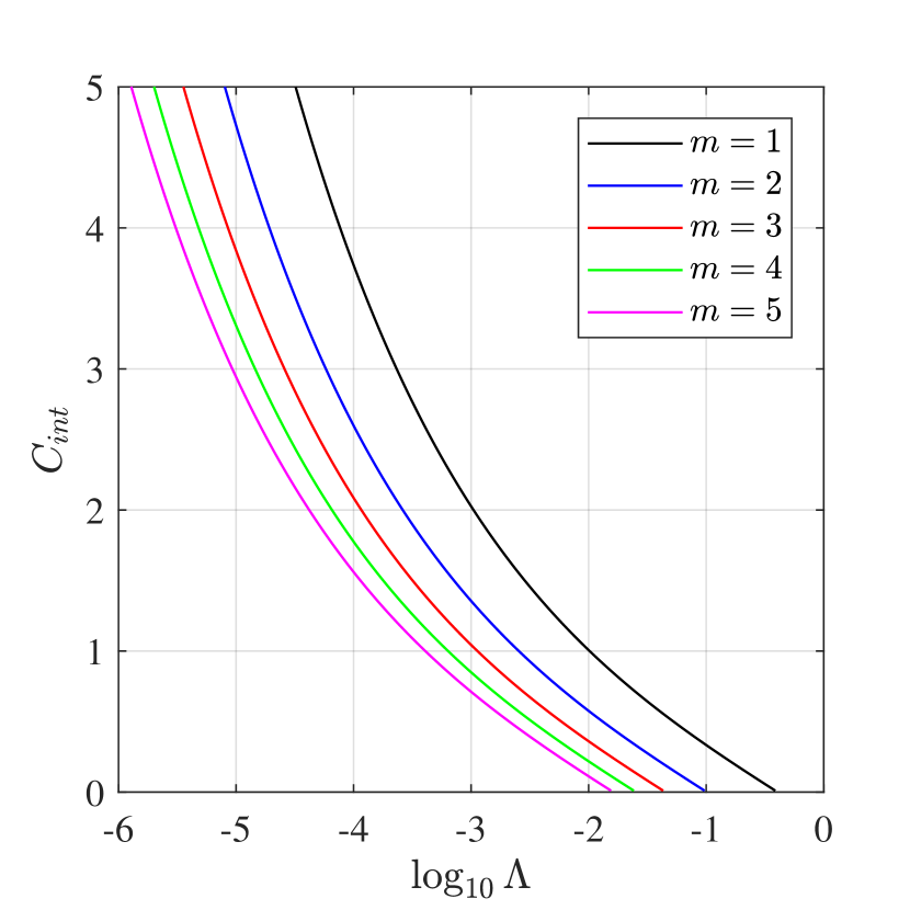
Figure 10: The location $C_{int}$ in the parameter space of Fig. 5 where the $\omega^{+}_{\mathit{lr}}$ intersects with $\omega_{c}$. This value decreases with both $\Lambda$ and $m$.

Finally, this interpretation in terms of minimum and maximum energy modes is related to another a curious feature of Fig. 5. When crossing $\omega^{+}_{\mathit{lr}}$ from below, the interacting modes can either couple or decouple depending on the position in the parameter space. The reason for this is that for $\omega_{c}<\omega_{\mathit{lr}}^{+}$, the light-ring involves the $+$ and $-$ modes which interact at an energy minimum; that is, as $\omega$ is increased, their propagation becomes classically allowed and the modes decouple. This is what is happening in the transition from type III to type I scattering. However, for $\omega_{c}>\omega_{\mathit{lr}}^{+}$, the light-ring involves the u and the $+$ modes which interact at an energy maximum; that is, as $\omega$ is increased, their propagation becomes classically forbidden and the modes become coupled. This is what happens in the transition from type II to IV as well as V to VI.

VI Conclusion

In this paper, a general scheme has been outlined to study the scattering of dispersive waves for which the equation of motion is of the form (1). The scheme is based on finding the paths traced out by the different modes through phase space, and identifying the locations where mode coupling takes place, i.e. at turning points and saddle points. This method was then applied to study the QNMs of weakly dispersive gravity waves around a hydrodynamic, rotating black hole analogue. This specific example was chosen due to it’s connection with recent experiments Torres et al. (2018a), however, it’s use is not limited to just this. Indeed, certain modifications to GR (e.g. Hořava gravity Sotiriou et al. (2011)) also exhibit modified dispersion relations which could be studied using the approach discussed here.

With particular regard to surface wave experiments involving draining vortices, there are a few comments to make. Fig. 4 illustrates that the range of possible interactions between dispersive modes is much richer than in the non-dispersive case where only two modes are present. This has implications for the superradiance experiment of Torres et al. (2017) which will be explored in another paper. In this work, the behaviour of the QNM spectrum was investigated, which is relevant to experiments of Torres et al. (2018a). It was shown in Section V.4, through a detailed analysis of the different scattering possibilities, that the well-known QNM condition in the non-dispersive case applies equally in the dispersive regime. Solving this condition led to the identification of two distinct behaviours: namely, the counter-rotating QNMs are barely affected by dispersion, whereas the co-rotating modes can depend strongly on it (similar conclusions were reached in Torres et al. (2018b) although a reason was not provided). This behaviour is related to the fact that, for co-rotating modes, different pairs of scattering channels are involved in the light-ring depending on the flow parameters. This leads to a different interpretation than that reached in Torres et al. (2018a), where it was suggested that the reason for the link between the QNMs and the light-ring modes is that the latter are the lowest frequency modes capable of transferring energy across the whole system. The present findings indicate that whilst this interpretation holds for the counter-rotating modes, the co-rotating QNMs (under certain circumstances) are actually more correctly identified with highest frequency modes capable of the same.

Given this observation, I can see two potential physical interpretations for the correspondence between the QNMs and the light-ring modes. The first is that the light-ring modes are those which can propagate deepest into the vortex core whilst avoiding reflection (this is visually apparent in both panels of Fig. 9). Hence, one would expect them to be the most efficient frequency band to transfer energy from inside the system to the outside. The second interpretation involves a brief thought experiment. Consider initialising the wave equation with random noise over the whole system. This will contain a superposition of all frequencies, which either enter the vortex core or propagate out to infinity as transients. There will be a particular frequency, however, corresponding to a particle that sits indefinitely at the stationary point of the effective potential curves in Fig. 9. In reality, the wave-like nature induces a decaying behaviour, as the mode slowly leaks away from the stationary point due to the spread of neighbouring trajectories there. In this sense, the QNMs are simply the modes which cling to the system the longest after it has been perturbed. Hopefully, these observations provide some new perspective on the link between the QNMs and the light-rings Cardoso et al. (2009), which has found use in the literature on many occasions e.g. in characterising fluid mechanical vortex flows Torres et al. (2019) and predicting gravitational waveforms in binary black hole mergers McWilliams (2019).

Finally, although in this work I have focussed on weakly dispersive gravity waves, the method can easily be extended to study the full dispersion relation for surface gravity waves including capillarity, see e.g. Torres et al. (2018a). Indeed, the method is sufficiently general that it can be applied to a wide variety of scattering problems, with potential application in both gravitational and condensed matter physics. I expect this will be particularly useful for the next generation of analogue gravity experiments, aiming to investigate general relativistic effects in evermore exotic settings, e.g. in Bose-Einstein condensates de Nova et al. (2019) and superfluid helium Človečko et al. (2019). The framework set out here provides simple, intuitive approach toward answering questions in these systems.

Appendix A Constrained Hamiltonian

Consider a mechanical system with $N$ generalised coordinates $q_{i}$ and momenta $p_{i}$. The Hamilton-Jacobi equation is a first order partial differential equation of the form [93],

$$-\partial_{t}S=H(q_{i},\partial_{q_{i}}S,t),$$ (A.1)

where $H=H(q_{i},p^{i},t)$ is the Hamiltonian. $S$ is Hamilton’s principle function defined as the indefinite integral of the Lagrangian $L$ with respect to $t$.

$$S(q,t)=\int^{(q,t)}Ldt,$$ (A.2)

which is related to the action functional $\mathcal{S}$ by fixing the initial point $(t_{0},q_{0})$ but allowing the upper limit of the integral to vary. The Lagrangian $L$ is related to the Hamiltonian by,

$$\begin{split}L=\frac{dS}{dt}=&\ \partial_{t}S+q^{\prime}_{i}\partial_{q_{i}}S,\\ =&\ \sum_{i=1}^{N}p_{i}q^{\prime}_{i}-H,\end{split}$$ (A.3)

where the dash denotes partial derivative with respect to $t$. This allows one to write the action for the system as,

$$\mathcal{S}=\int dt\left(\sum_{i=1}^{N}p_{i}q^{\prime}_{i}-H\right).$$ (A.4)

The action can be put in parametrised form by regarding the time $t$ as a new coordinate $q_{N+1}$ which is parametrised by (say) $\tau$ [85],

$$\mathcal{S}=\int d\tau\left(\sum_{i=1}^{N+1}p_{i}\dot{q}_{i}\right),$$ (A.5)

where overdot denotes derivative with respect to $\tau$. One also needs to make sure that the constraint equation $p_{N+1}+H=0$ holds. This can be implemented by adding a term to the action,

$$\mathcal{S}=\int d\tau\left(\sum_{i=1}^{N+1}p_{i}\dot{q}_{i}-\alpha(\tau)\mathcal{H}\right),$$ (A.6)

where $\alpha$ is a Lagrange multiplier, which is an arbitrary function of $\tau$. Requiring that $\mathcal{S}$ be stationary when $\alpha$ is varied yields the constraint $\mathcal{H}=0$, where $\mathcal{H}$ can be any function whose root is $p_{N+1}=-H$. In this picture, $\mathcal{H}$ appears as an effective Hamiltonian.

Now, notice that the WKB phase is precisely of the form (A.2) with coordinates $\mathbf{x}$ and momenta $\mathbf{k}$. Using the Hamilton-Jacobi equation (A.1) with the definition in (14), one can see that the Hamiltonian $H$ is given by $\omega_{D}^{\pm}$ defined in (10). Thus, the effective Hamiltonian $\mathcal{H}$ must yield $\omega=\omega_{D}^{\pm}$ as it’s roots. The function defined in (15) gives precisely this.

Appendix B Transfer matrix at turning points

In this appendix, I outline the derivation of the derivation of transfer matrices $T$ and $\widetilde{T}$ defined in (30) and (31) respectively, as well as the two turning point matrix $\mathcal{N}_{ab}$ in (33). To begin, the effective Hamiltonian is expanded around the turning point,

$$\mathcal{H}=\partial_{r}\mathcal{H}_{tp}(r-r_{tp})+\tfrac{1}{2}\mathcal{H}^{\prime\prime}_{tp}(p-p_{tp})^{2},$$ (B.1)

where the turning point conditions in (28) have been applied. Promoting $p\to-i\partial_{r}$ and applying the on-shell condition, (B.1) becomes the local wave equation,

$$-\partial_{r}^{2}\psi+2ip_{tp}\partial_{r}\psi+\left[p^{2}_{tp}+Q(r-r_{tp})\right]\psi=0,$$ (B.2)

where $Q=2\partial_{r}\mathcal{H}_{tp}/\mathcal{H}^{\prime\prime}_{tp}$ which is a constant factor determined by the properties of the turning point. Note that $Q$ increases with $|m|$. The general solution to (B.2) is,

$$\psi=e^{ip_{tp}r}\left[C_{1}\mathrm{Ai}\left(s\right)+C_{2}\mathrm{Bi}\left(s\right)\right],$$ (B.3)

where $\mathrm{Ai}(s)$ and $\mathrm{Bi}(s)$ are the two linearly independent solutions of Airy’s equation [94], $C_{1,2}$ are constants and $s=Q^{1/3}(r-r_{tp})$. Far from the turning point, i.e. in the limits $s\to\pm\infty$, these asymptote to,

$$\begin{split}\mathrm{Ai}(s)&\underset{-\infty}{\sim}\frac{1}{2|s|^{1/4}\sqrt{\pi}}\Big{(}e^{-i\frac{2}{3}(-s)^{3/2}+i\frac{\pi}{4}}+e^{i\frac{2}{3}(-s)^{3/2}-i\frac{\pi}{4}}\Big{)},\\ &\underset{+\infty}{\sim}\frac{e^{-\frac{2}{3}s^{3/2}}}{2|s|^{1/4}\sqrt{\pi}},\\ \mathrm{Bi}(s)&\underset{-\infty}{\sim}\frac{i}{2|s|^{1/4}\sqrt{\pi}}\Big{(}e^{i\frac{2}{3}(-s)^{3/2}-i\frac{\pi}{4}}-e^{-i\frac{2}{3}(-s)^{3/2}+i\frac{\pi}{4}}\Big{)},\\ &\underset{+\infty}{\sim}\frac{e^{\frac{2}{3}s^{3/2}}}{|s|^{1/4}\sqrt{\pi}}.\\ \end{split}$$ (B.4)

Next, one must find the form of the WKB solutions close to the turning point. First, solving (B.1) for $\mathcal{H}=0$ yields the radial wavevector in terms of $s$,

$$p=p_{tp}\pm Q^{\frac{1}{3}}(-s)^{\frac{1}{2}}.$$ (B.5)

Also using (B.1) to compute the leading contribution to to the amplitude (22), the WKB solution is of the form,

$$\frac{e^{ip_{\mathit{tp}}r}}{|s|^{1/4}}e^{\pm\frac{2}{3}i(-s)^{\frac{3}{2}}}.$$ (B.6)

Now, consider the scenario where the modes are oscillatory for $s<0$ and evanescent for $s>0$. The solution either side of the turning point is,

$$\begin{split}\psi(s<0)=&\ \alpha^{\mathrm{R}}\psi^{\mathrm{R}}(s)+\alpha^{\mathrm{L}}\psi^{\mathrm{L}}(s),\\ \psi(s>0)=&\ \alpha^{\downarrow}\psi^{\downarrow}(s)+\alpha^{\uparrow}\psi^{\uparrow}(s).\end{split}$$ (B.7)

where the WKB modes are defined,

$$\begin{split}\psi^{\mathrm{L}}\simeq\frac{e^{-i\frac{2}{3}(-s)^{3/2}}}{2|s|^{1/4}\sqrt{\pi}},\qquad\psi^{\mathrm{R}}\simeq\frac{e^{i\frac{2}{3}(-s)^{3/2}}}{2|s|^{1/4}\sqrt{\pi}},\\ \psi^{\uparrow}\simeq\frac{e^{\frac{2}{3}s^{3/2}}}{2|s|^{1/4}\sqrt{\pi}},\qquad\psi^{\downarrow}\simeq\frac{e^{-\frac{2}{3}s^{3/2}}}{2|s|^{1/4}\sqrt{\pi}}.\end{split}$$ (B.8)

Equating (B.7) with (B.3) in the asymptotic limits given by (B.4), one finds a relation between the amplitudes $C_{1,2}$ and the different $\alpha$’s. Eliminating the $C_{1,2}$ gives,

$$\begin{split}\alpha^{\mathrm{R}}=&\ e^{i\pi/4}\alpha^{\downarrow}+\tfrac{1}{2}e^{-i\pi/4}\alpha^{\uparrow},\\ \alpha^{\mathrm{L}}=&\ e^{-i\pi/4}\alpha^{\downarrow}+\tfrac{1}{2}e^{i\pi/4}\alpha^{\uparrow},\end{split}$$ (B.9)

which are equivalent to the matrix equation (30) in the main text. To obtain the transfer matrix in the mirror situation (i.e. evanescent solutions for $s<0$ and oscillatory for $s>0$) one needs to make the transformation $s\to-s$ in (B.3) and (B.7). Repeating the same procedure, one finds,

$$\begin{split}\alpha^{\uparrow}=\ &\tfrac{1}{2}e^{i\pi/4}\alpha^{\mathrm{R}}+\tfrac{1}{2}e^{-i\pi/4}\alpha^{\mathrm{L}}\\ \alpha^{\downarrow}=\ &e^{-i\pi/4}\alpha^{\mathrm{R}}+e^{i\pi/4}\alpha^{\mathrm{L}}\end{split}$$ (B.10)

which are equivalent to the matrix equation (31) in the main text. The mode labelled by $\uparrow$ is the one that grows in the direction of increasing $r$ in both cases. Note that (B.10) is not simply a rearrangement of (B.9) since the amplitudes are defined in different scenarios. Rearranging (B.9) for the evanescent amplitudes would give the correct transfer matrix but in the opposite direction. To correct for this, one would need to exchange the role of the $\mathrm{R}$ and $\mathrm{L}$ modes. This means that $\widetilde{T}$ is not the inverse of $T$ but the conjugate inverse, i.e. $\widetilde{T}=(T^{*})^{-1}$.

The two turning point conversion matrix is obtained by applying $T$ at $r_{a}$ and $\tilde{T}$ at $r_{b}$ with a matrix containing the WKB shift factors (27) in between. The modes are evanescent in the region $r_{a}<r<r_{b}$ and are labelled $p^{\uparrow}$ and $p^{\downarrow}$,

$$\begin{pmatrix}A_{a}^{\mathrm{R}}\\ A_{a}^{\mathrm{L}}\end{pmatrix}=T\begin{pmatrix}0&\mathcal{F}_{ab}^{\downarrow}\\ \mathcal{F}_{ab}^{\uparrow}&0\end{pmatrix}\widetilde{T}\begin{pmatrix}A_{b}^{\mathrm{R}}\\ A_{b}^{\mathrm{L}}\end{pmatrix}.$$ (B.11)

Between the turning points, the radial wavevectors satisfy $\mathrm{Re}[p^{\uparrow}]=\mathrm{Re}[p^{\downarrow}]$ and $\mathrm{Im}[p^{\uparrow}]=-\mathrm{Im}[p^{\downarrow}]<0$. One also has $|\mathcal{H}^{\prime}(p^{\uparrow})|=|\mathcal{H}^{\prime}(p^{\downarrow})|$. Using these relations, (B.11) becomes (32) in the main text.

Appendix C Transfer matrix at a saddle point

In this appendix, I detail the derivation of the saddle point conversion matrix $\mathcal{S}$ defined in (36) (see also [83]). The derivation begins by expanding the effective Hamiltonian about the saddle point,

$$\mathcal{H}=\mathcal{H}_{\mathit{sp}}+\partial_{r}\partial_{p}\mathcal{H}_{\mathit{sp}}\delta r\delta p+\tfrac{1}{2}\partial_{r}^{2}\mathcal{H}_{\mathit{sp}}\delta r^{2}+\tfrac{1}{2}\partial_{p}^{2}\mathcal{H}_{\mathit{sp}}\delta p^{2},$$ (C.1)

where $\delta r=r-r_{\mathit{sp}}$ and $\delta p=p-p_{\mathit{sp}}$ and the saddle point conditions in (34) have been applied. Note in particular that whilst $\mathcal{H}$ vanishes for the solutions to the dispersion relation, $\mathcal{H}_{\mathit{sp}}$ does not necessarily.

Compared to the turning point problem of Appendix B, the present case is more complicated by the presence of the cross term proportional to $\delta r\delta p$. This term can be eliminate by a change of coordinate basis in the $(r,p)$ plane. First, rewrite (C.1) as,

$$\mathcal{H}=\mathcal{H}_{\mathit{sp}}+\tfrac{1}{2}\mathbf{Y}^{\mathrm{T}}[\mathrm{d}^{2}\mathcal{H}]\mathbf{Y},$$ (C.2)

where,

$$[\mathrm{d}^{2}\mathcal{H}]=\begin{pmatrix}\partial_{r}^{2}\mathcal{H}_{\mathit{sp}}&\partial_{r}\partial_{p}\mathcal{H}_{\mathit{sp}}\\ \partial_{r}\partial_{p}\mathcal{H}_{\mathit{sp}}&\partial_{p}^{2}\mathcal{H}_{\mathit{sp}}\end{pmatrix},$$ (C.3)

is the Hessian matrix and the coordinate vector is,

$$\mathbf{Y}=\begin{pmatrix}\delta r\\ \delta p,\end{pmatrix}$$ (C.4)

with $\mathbf{Y}^{\mathrm{T}}$ it’s transpose. The change of basis in the $(r,p)$ plane proceeds via the standard method. The eigenvalues of $[\mathrm{d}^{2}\mathcal{H}]$ are given by,

$$\begin{split}\mu_{\pm}=\ &\tfrac{1}{2}\Big{(}\partial_{r}^{2}\mathcal{H}_{\mathit{sp}}+\partial_{p}^{2}\mathcal{H}_{\mathit{sp}}\pm\mathrm{sgn}(\partial_{p}^{2}\mathcal{H}_{\mathit{sp}})\times\\ &\sqrt{(\partial_{r}^{2}\mathcal{H}_{\mathit{sp}}-\partial_{p}^{2}\mathcal{H}_{\mathit{sp}})^{2}+4(\partial_{r}\partial_{p}\mathcal{H}_{\mathit{sp}})^{2}}\Big{)}.\end{split}$$ (C.5)

Next, $[\mathrm{d}^{2}\mathcal{H}]$ can be put into the form,

$$[\mathrm{d}^{2}\mathcal{H}]=\begin{pmatrix}\cos\theta&-\sin\theta\\ \sin\theta&\cos\theta\end{pmatrix}\begin{pmatrix}\mu_{-}&0\\ 0&\mu_{+}\end{pmatrix}\begin{pmatrix}\cos\theta&\sin\theta\\ -\sin\theta&\cos\theta,\end{pmatrix}$$ (C.6)

where the rotation angle is defined,

$$\theta=\tan^{-1}\left(\frac{\mu_{-}-\partial_{r}^{2}\mathcal{H}_{\mathit{sp}}}{\partial_{r}\partial_{p}\mathcal{H}_{\mathit{sp}}}\right).$$ (C.7)

Defining new coordinates $(R,P)$ via,

$$\begin{pmatrix}R\\ P\end{pmatrix}=\begin{pmatrix}\cos\theta&\sin\theta\\ -\sin\theta&\cos\theta\end{pmatrix}\begin{pmatrix}\delta r\\ \delta p\end{pmatrix}$$ (C.8)

the Hamiltonian becomes,

$$\mathcal{H}=\mathcal{H}_{\mathit{sp}}+\tfrac{1}{2}\mu_{-}R^{2}+\tfrac{1}{2}\mu_{+}P^{2}.$$ (C.9)

Note, in particular, that due to the definition of the eigenvalues in (C.5), the sign of the $P^{2}$ term in (C.9) coincides with that of $\delta p^{2}$ in the original Hamiltonian of (C.1). Finally, the Hamiltonian is scaled by a factor $\sqrt{-\mu_{+}\mu_{-}}$ and the scaled coordinates are defined,

$$X=\sqrt{\frac{-\mu_{-}}{\mu_{+}}}R,\qquad K=\sqrt{\frac{-\mu_{+}}{\mu_{-}}}P,$$ (C.10)

which puts the scaled Hamiltonian $\overline{\mathcal{H}}$ in the form,

$$\overline{\mathcal{H}}=b-\tfrac{1}{2}X^{2}+\tfrac{1}{2}K^{2}.$$ (C.11)

The relative minus sign between the $X^{2}$ and $K^{2}$ terms has appeared because $\mu_{+}\mu_{-}<0$ due to the saddle point structure, and $b$ is defined,

$$b=\frac{\mathrm{sgn}(\mathcal{H}^{\prime\prime}_{\mathit{sp}})\mathcal{H}_{\mathit{sp}}}{\sqrt{-\mu_{+}\mu_{-}}}.$$ (C.12)

Note that $\mu_{+}\mu_{-}=\mathrm{det}[\mathrm{d}^{2}\mathcal{H}]$.

To obtain the local form of the wave equation, one makes the identification $K=-i\partial_{X}$ which, applying the on-shell condition, leads to,

$$\left[b-\tfrac{1}{2}\left(X^{2}+\partial_{X}^{2}\right)\right]\psi=0,$$ (C.13)

whose general solution may be written as,

$$\psi=C_{1}U(ib,\sqrt{2}Xe^{-i\pi/4})+C_{2}U(-ib,\sqrt{2}Xe^{i\pi/4}),$$ (C.14)

where $U(a,z)$ is the parabolic cylinder function [95]. The goal is now to match the asymptotic form of this exact solution onto the WKB modes far from the saddle point. First one must evaluate the WKB phase. $K$ is obtained from (C.11) with $\overline{\mathcal{H}}=0$, from which one has,

$$\int KdX\underset{|X|\gg|b|}{\sim}\pm\left(\tfrac{1}{2}X^{2}-b\log|X|\right),$$ (C.15)

where the $+$ ($-$) sign is taken for $X>0$ ($X<0$). The factor in the WKB amplitude in the same limit is $|\mathcal{H}^{\prime}|^{\frac{1}{2}}\sim|X|^{\frac{1}{2}}$. Hence, the different WKB modes are,

$$\begin{split}\psi_{<}^{\mathrm{L}}\simeq e^{iX^{2}/2}|X|^{-ib-\frac{1}{2}},&\ \qquad\psi_{<}^{\mathrm{R}}\simeq e^{-iX^{2}/2}|X|^{ib-\frac{1}{2}},\\ \psi_{>}^{\mathrm{L}}\simeq e^{-iX^{2}/2}|X|^{ib-\frac{1}{2}},&\ \qquad\psi_{>}^{\mathrm{R}}\simeq e^{iX^{2}/2}|X|^{-ib-\frac{1}{2}},\end{split}$$ (C.16)

and the full solution in each region is,

$$\begin{split}\psi(X<0)=&\ \alpha^{\mathrm{R}}_{<}\psi_{<}^{\mathrm{R}}+\alpha^{\mathrm{L}}_{<}\psi_{<}^{\mathrm{L}},\\ \psi(X>0)=&\ \alpha^{\mathrm{R}}_{>}\psi_{>}^{\mathrm{R}}+\alpha^{\mathrm{L}}_{>}\psi_{>}^{\mathrm{L}}.\end{split}$$ (C.17)

The asymptotic form of the parabolic cylinder functions is given in [80]. In the present case, this gives,

$$\begin{split}U(ib,\sqrt{2}Xe^{-i\pi/4})\underset{X\to-\infty}{\sim}\ &(e^{3i\pi/4})^{-ib-\frac{1}{2}}\left[e^{iX^{2}/2}|\sqrt{2}X|^{-ib-\frac{1}{2}}+\frac{\sqrt{2\pi}}{\Gamma(\frac{1}{2}+ib)}e^{-\pi b/2+i\pi/2}e^{-iX^{2}/2}|\sqrt{2}X|^{ib-\frac{1}{2}}\right],\\ \underset{X\to\infty}{\sim}\ &(e^{3i\pi/4})^{-ib-\frac{1}{2}}e^{iX^{2}/2}|\sqrt{2}X|^{-ib-\frac{1}{2}}e^{-\pi b-i\pi/2},\\ U(-ib,\sqrt{2}Xe^{i\pi/4})\underset{X\to-\infty}{\sim}\ &(e^{-3i\pi/4})^{ib-\frac{1}{2}}\left[e^{-iX^{2}/2}|\sqrt{2}X|^{ib-\frac{1}{2}}-\frac{\sqrt{2\pi}}{\Gamma(\frac{1}{2}-ib)}e^{-\pi b/2+i\pi/2}e^{iX^{2}/2}|\sqrt{2}X|^{-ib-\frac{1}{2}}\right],\\ \underset{X\to\infty}{\sim}\ &(e^{-3i\pi/4})^{ib-\frac{1}{2}}e^{-iX^{2}/2}|\sqrt{2}X|^{ib-\frac{1}{2}}e^{-\pi b-i\pi/2}.\end{split}$$ (C.18)

The final step involves equating (C.17) with (C.14) in the asymptotic limits given by (C.18). This yields a relation between the amplitudes $C_{1,2}$ and the different $\alpha$’s. Substituting out $C_{1,2}$ yields the following relations,

$$\begin{split}\alpha_{<}^{\mathrm{L}}=&\ i\tau^{-1}\left(-\alpha_{>}^{\mathrm{R}}+2^{-ib}e^{-i\pi/4}\beta^{*}\alpha_{>}^{\mathrm{L}}\right),\\ \alpha_{<}^{\mathrm{R}}=&\ i\tau^{-1}\left(-2^{ib}e^{i\pi/4}\beta\alpha_{>}^{\mathrm{R}}+\alpha_{>}^{\mathrm{L}}\right),\end{split}$$ (C.19)

where $\beta$ and $\tau$ are defined in (36) of the main text. These two relations give precisely the conversion matrix $\mathcal{S}$ in (35).