Landslide Segmentation with U-Net: Evaluating Different Sampling Methods and Patch Sizes

Abstract

Landslide inventory maps are crucial to validate predictive landslide models; however, since most mapping methods rely on visual interpretation or expert knowledge, detailed inventory maps are still lacking. This study used a fully convolutional deep learning model named U-net to automatically segment landslides in the city of Nova Friburgo, located in the mountainous range of Rio de Janeiro, southeastern Brazil. The objective was to evaluate the impact of patch sizes, sampling methods, and datasets on the overall accuracy of the models. The training data used the optical information from RapidEye satellite, and a digital elevation model (DEM) derived from the L-band sensor of the ALOS satellite. The data was sampled using random and regular grid methods and patched in three sizes (32x32, 64x64, and 128x128 pixels). The models were evaluated on two areas with precision, recall, f1-score, and mean intersect over union (mIoU) metrics. The results show that the models trained with 32x32 tiles tend to have higher recall values due to higher true positive rates; however, they misclassify more background areas as landslides (false positives). Models trained with 128x128 tiles usually achieve higher precision values because they make less false positive errors. In both test areas, DEM and augmentation increased the accuracy of the models. Random sampling helped in model generalization. Models trained with 128x128 random tiles from the data that used the RapidEye image, DEM information, and augmentation achieved the highest f1-score, 0.55 in test area one, and 0.58 in test area two. The results achieved in this study are comparable to other fully convolutional models found in the literature, increasing the knowledge in the area.

Keywords Deep Learning  $\cdot$ Fully Convolutional Networks (FCN)  $\cdot$ Nova Friburgo  $\cdot$ RapidEye  $\cdot$ Landslide mapping

1 Introduction

Natural hazards are more frequent and harmful in recent years due to unplanned urbanization, climate change, and population growth (Kobiyama et al., 2006; Hong et al., 2017; Alexander, 2008; Zhong et al., 2019). According to the Sendai framework for disaster risk reduction 2015-2030 (UNISDR, 2015), between 2008 and 2012, those hazards affected more than 25 million people, with an economic loss of about 1.3 trillion dollars, impeding the progress towards sustainable development.

Landslides commonly cause victims, damages to human habitations, and economic losses. Therefore, the study of landslide detection has been considered a critical area of research in remote sensing (Hong et al., 2017). However, despite the importance highlighted by many authors, detailed landslides inventories are still lacking (Mondini et al., 2019; Guzzetti et al., 2012). Landslide inventory maps are used to prepare and validate landslide susceptibility models, evaluate risk and vulnerability, study erosion and geomorphology, and document the impact of a landslide disaster (Van Westen et al., 2008). Limited and incomplete data may be a source of bias for these studies since model success depends directly on inventory accuracy.

Landslides inventory maps usually are prepared by using remote sensing imagery with high (HR) and very-high (VHR) resolution (Zhong et al., 2020). The landslides can be recognized in an aerial image manually by visual interpretation, semi-automatically, or automatically by using algorithms for object image analysis (OBIA) and pixel-based classification. Manual classification of landslides is the prevailing method (Xu, 2015; Yu et al., 2020), but, for large areas, it is time-consuming. OBIA methodologies classify landslide areas by grouping objects with similar spectral, spatial, hierarchical, textural, and morphological properties (Blaschke, 2010). Nevertheless, the assignment of those parameters is highly dependent on the analyst experience. Pixel-based methodologies classify each pixel of the image based on its spectral information. However, geometric and contextual information present in the image is ignored, increasing the salt-and-pepper noise in the results (Stumpf and Kerle, 2011; Blaschke et al., 2014; Zhong et al., 2019; Prakash et al., 2020).

In recent years, deep convolution neural networks (DCNN) achieve state-of-art results in applications such as semantic segmentation, object detection, natural language processing, and speech recognition (Ghorbanzadeh et al., 2019; Peng et al., 2019; Zhu et al., 2017; Long et al., 2015; Radovic et al., 2017). However, only a few studies have used DCNNs for landslide detection (Zhong et al., 2020).

Ding et al. (2016) used DCNN on GF-1 (Gaofen-1) images with four spectral bands and eight-meter resolution, achieving an overall accuracy of 67%, a detection rate of 72.5%, and 10.2% of false positive rate. Chen et al. (2018) used DCNN on bi-temporal images to evaluate areas with drastic changes and combined a spatial context learning (STCL) and information from a digital elevation model (DEM) to detect landslide areas. The method yield an accuracy of more than 61% on the evaluated areas. Ghorbanzadeh et al. (2019) compared state-of-art machine learning methods and DCNN on RapidEye images and a DEM, with five meters of spatial resolution. The DCNN that used only spectral information and small windows was the best model achieving 78.26% on the mean intersect over union (mIoU) metric. Sameen and Pradhan (2019) compared residual networks (ResNets) trained with topographical information fused using convolutional networks with topographical data added as additional channels. The models trained with the fused data achieved f1-score and mIoU that were superior by 13% and 12.96% compared to the other models. Yu et al. (2020) used the enhanced vegetation index (EVI), DEM degradation indexes, and a contouring algorithm on Landsat images to sample potential landslide zones with less class imbalance distribution. The trained fully convolutional network (PSPNet) achieved 65% of recall and 55.35% of precision. Prakash et al. (2020) used Lidar DEM and Sentinel-2 images to compare traditional pixel, object, and DCNN methods. The deep learning method, U-net with ResNet34 blocks, achieved the best results with the Matthews correlation coefficient score of 0.495 and the probability of detection rate of 0.72.

DCNNs, in supervised learning problems, can learn to identify patterns on the training data without the need for complex operations to extract features or preprocessing methods. However, choosing the best network architecture, preparing the training dataset, and tuning the hyperparameters is still a challenge (Pradhan et al., 2017; Sameen and Pradhan, 2019). Landslides scars dataset usually have an imbalanced class distribution with more pixels belonging to background objects, such as urban areas, vegetation, and water, than landslide scars (Yu et al., 2020). Therefore, since landslide scars have different shapes and sizes, sampling methods and patch sizes may affect the model accuracy as it can be a way to reduce the class imbalance between the positive and the negative class.

This research aims to evaluate how different datasets, sampling methods, and patch sizes impacts on the landslide segmentation accuracy of U-net. To achieve that, we trained 288 models with landslide optical information from a RapidEye satellite and topographical information from a DEM derived from the Phased Array type L-band Synthetic Aperture Radar (PALSAR) sensor of the ALOS satellite. The models were trained with images patched in three different sizes (32x32, 64x64, 128x128 pixels), and sampled using random and regular grid sampling methods. Data augmentation was also tested. The study area is in the city of Nova Friburgo, located in the mountainous range of Rio de Janeiro, Brazil. The models were evaluated in two test areas with f1-score, recall, precision, and mean intersect over union (mIoU) metrics.

The main contributions of this research are as follows:

• Broad comparison between patch sizes, sampling method, and datasets.

• Evaluation of U-net architecture for semantic segmentation of landslides.

2 Study Area

In January 2011, an extreme rainfall event (350 mm/48h) triggered at least 3500 translational landslides that killed more than 1500 people and disrupted all major city facilities in the mountainous region of Rio de Janeiro, Brazil. This event is considered the worst Brazilian natural disaster (Avelar et al., 2013).

The mountainous region of Rio de Janeiro encompasses the municipalities of Nova Friburgo, Teresópolis, Petrópolis, Sumidouro, São José do Vale do Rio Preto and Bom Jardim (Fig. 1). The study area is in the municipality of Nova Friburgo, which was severely damaged by the disaster.

Nova Friburgo is in the geomorphological unit of Serra dos Orgãos. The geological units have a WSW-ENE trend, and the elevation ranges between 1100 and 2000 meters above the mean sea level (Dantas, 2001). The geology consists mainly of igneous and metamorphic rocks such as granites, diorites, gabbros, and gneisses (Tupinambá et al., 2012). According to Köppen’s climate classification scheme (Köppen, 1936), the climate is subtropical highland (Cwb) with dry winter and mild summers. The annual mean precipitation is 1585.62 mm, with most of the rainfall in November, December, and January (Sobral et al., 2018).

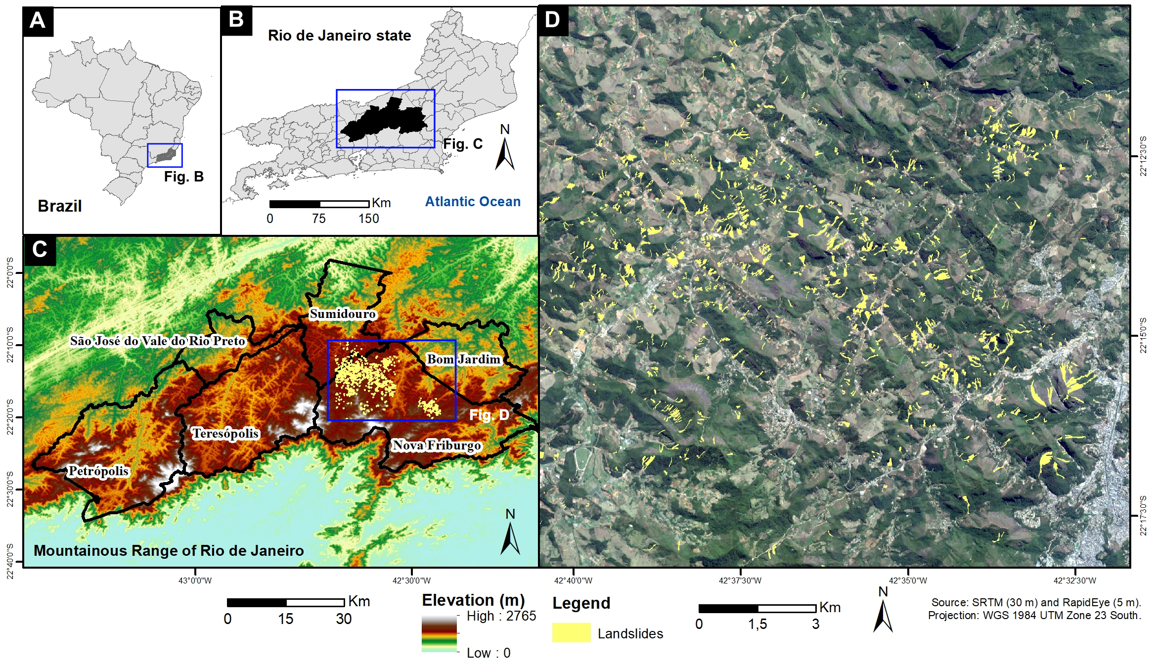
Figure 1: A) Location of the study area in southeastern Brazil. B) Location of the Mountainous Range in the Rio de Janeiro State. C) Mountainous Range of Rio de Janeiro with the study area highlighted in blue. D) True color composition of the RapidEye image over Nova Friburgo, with the segmented landslides in yellow. The image was acquired on 2011-08-13.

3 Methodology

The spectral information from a RapidEye image and topographical information from a digital elevation model (DEM) derived from the ALOS’s Phased Array L-band Synthetic Aperture Radar (PALSAR) were used to evaluate the performance of the U-net on landslide segmentation. The models were trained with images in three different window dimensions (32x32, 64x64, 128x128 pixels) that were sampled using random and regular grid methods. Random rotation, vertical, and horizontal flip were used for data augmentation. In total, 288 models were trained (Table 1).

Table 1: Number of trained models on each dataset.

# of Models	Dataset
72	RapidEye
72	RapidEye + Augmentation
72	RapidEye + DEM
72	RapidEye + DEM + Augmentation

The model’s performance was evaluated in two test areas by using the mean intersect over union (mIoU), f1-score, precision, and recall metrics. The proposed methodology involves the following steps: (1) data preprocessing, (2) model training (3) model evaluation.

3.1 Data Preprocessing

3.1.1 RapidEye

RapidEye consists of a constellation of five identical satellites with high-resolution sensors with a 6.5 meters nominal ground sampling distance at nadir. The orthorectified products are resampled and provided to users at a pixel size of 5 meters. The data are acquired with a temporal resolution of 5 days in five spectral bands: blue (440–510 nm), green (520–590 nm), red (630–685 nm), red-edge (690–730 nm), near-infrared (760–850 nm) (RapidEye, 2011).

This work used the raw digital number (DN) of a 3A product (orthorectified, radiometric, and geometric corrections) with an area of 625 km². The image was acquired on 13 August 2011 and downloaded from the Planet Explorer website (Planet Team, 2017).

3.1.2 ALOS/PALSAR

The Phased Array type L-band Synthetic Aperture Radar (PALSAR) is one of the three observation sensors of the Advanced Land Observing Satellite (ALOS). PALSAR data is acquired at an off-nadir angle of 34.3 degrees in a Sun-synchronous Sub-recurrent Orbit (SSO) with a 46-day recurrent period.

In this study, we used the radiometric terrain correction (RTC) product with 12.5 meters of spatial resolution obtained from the Alaska Satellite Facility (ASF) (DAAC, 2015). The image was acquired on 28 January 2011. The data were resampled to 5 meters pixel resolution with bilinear interpolation method, to match the spatial resolution of the RapidEye image, using GRASS GIS version 7.2.2 (Neteler et al., 2012; GRASS Development Team, 2017).

3.1.3 Data Labeling

The landslides were manually labeled in the RapidEye image using QGIS version 3.8 (QGIS Development Team, 2009). The segmented landslides were validated with Google Earth Pro version 7.3 (Google, 2019) and by comparison with the landslide map produced by (Netto et al., 2013). In total, 1007 landslides were extracted from the scene, with area ranging from 200.32 m² to 78117.35 m² (638.51 m² average).

3.1.4 Test Areas

The model’s accuracy was evaluated in two test areas with 1024x1024 pixels (Fig. 2). In the first area, agriculture and grazing are predominant, while in the second, native vegetation and human settlements predominate. Ninety-six landslides were extracted from the first area and ninety-one from the second.

3.1.5 Binary Mask

The landslide scars polygons from the train and test areas were rasterized with Rasterio (Gillies et al., 2013–) and Numpy (Oliphant, 2006) Python libraries, to generate a binary mask with the same dimensions of the original scene. The pixels assigned with the value 1 (white pixels) correspond to the landslide scars class and the value 0 (black pixels) to the background class.

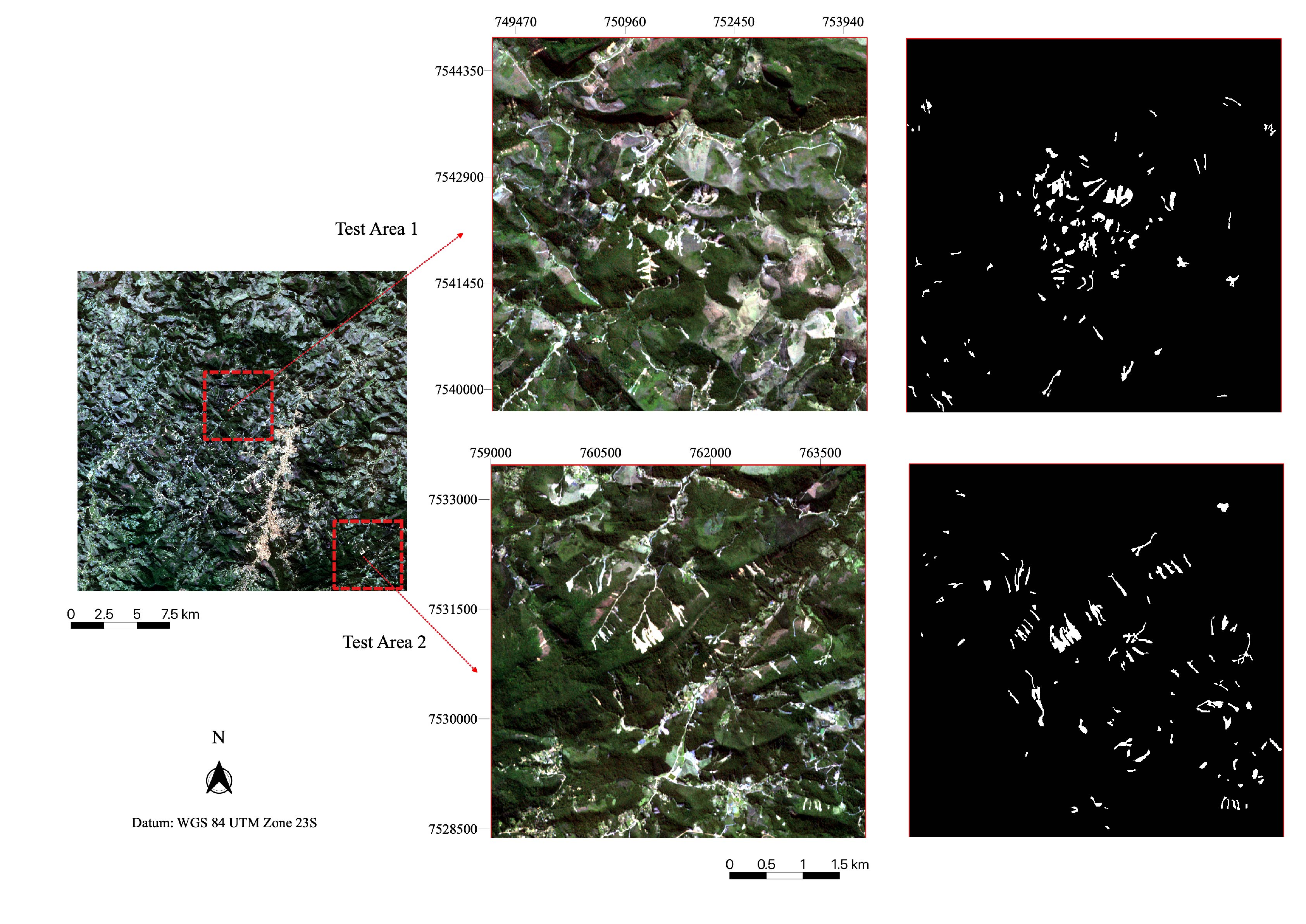
Figure 2: Location of test areas and their binary masks. White pixels represent the manually segmented landslides and black pixels the background.

3.1.6 Sampling Methods and Patch Sizes

The data was sampled by using random and regular grid methods in three different sizes: 32x32, 64x64, 128x128 pixels (Fig. 3).

The grid method used the bounding coordinates and the image resolution (5 meters) to generate a vector grid. The squares over the grid have an overlap of 20%. The random sampling used the same procedure to generate 5000 sampling square polygons. A select-by-location operation was used to select only the polygons intersecting landslides. This ensures that all sampled images will have at least a small portion of a landslide scar, reducing class imbalance. The code used was adapted from the Keras-Spatial library (Terstriep, 2019).

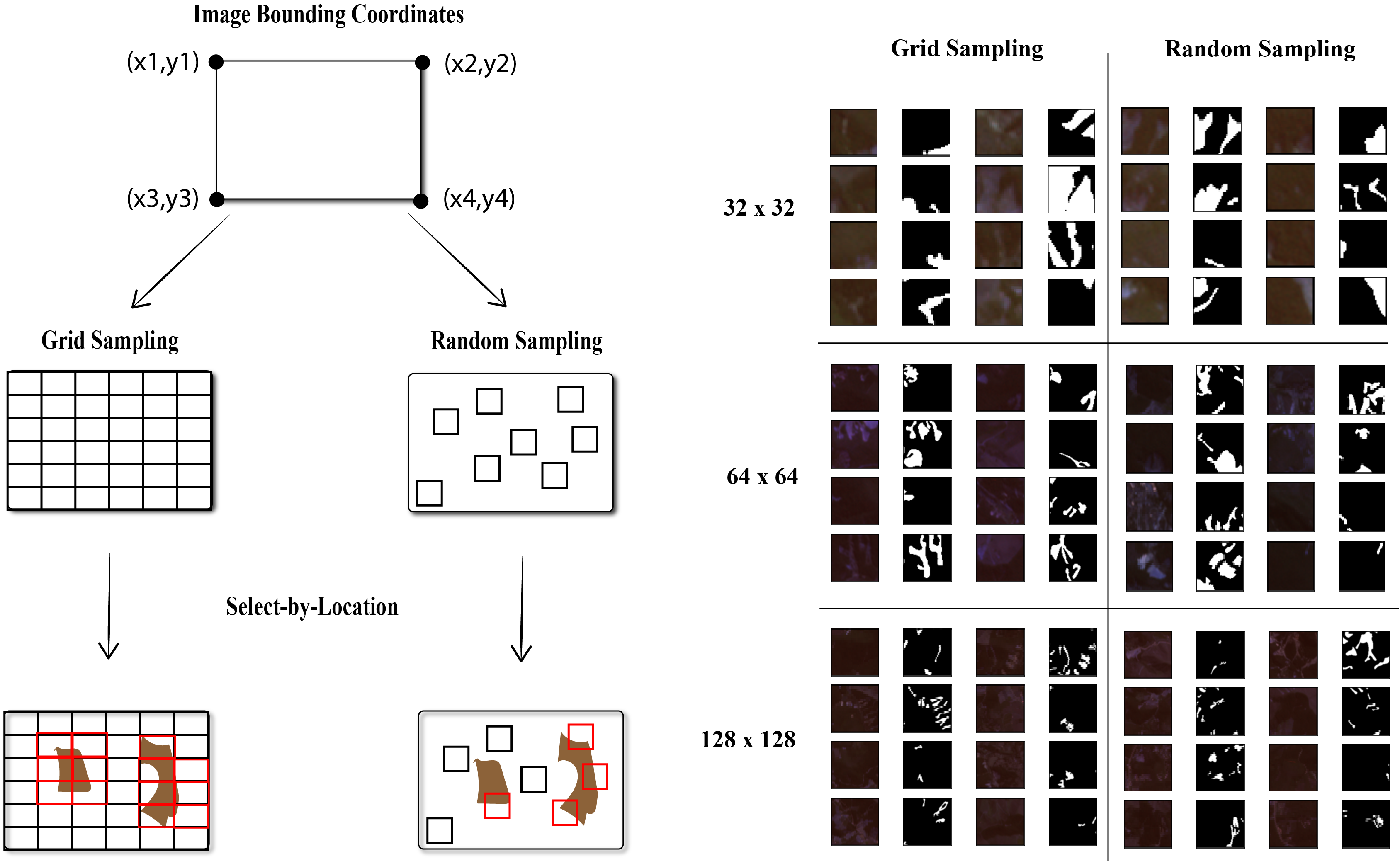
Figure 3: Sampling methods (left) and results obtained for each patch size (right).

3.1.7 Data Augmentation

The Albumentation library (Buslaev et al., 2018) was used to augment the data by using random rotations around 90^∘, vertical, and horizontal flips. Table 2 shows the sizes of all the datasets used to train the models.

Table 2: Number of samples from all the datasets and patch sizes used to train the models.

Dataset	Size (pixels)	Regular Sampling	Random Sampling
RapidEye	32x32	3541	1740
	64x64	2264	2368
RapidEye + DEM	128x128	1565	3653
RapidEye + Augmentation	32x32	9912	4872
	64x64	6336	6628
RapidEye + DEM + Augmentation	128x128	4380	10228

3.2 Model Training

3.2.1 Model Architecture

U-net (Ronneberger et al., 2015) is a fully convolutional network developed for the segmentation of biomedical images. This type of architecture does not use fully connected layers in their structure; instead, they have an encoder-decoder architecture with just convolutional layers. The encoder path is responsible for classifying the pixels, but without taking the spatial location into account. The decoder path uses up-convolutions and concatenation to recover the spatial location of the classified pixels and return a mask with the same dimensions of the input image.

In this study, we evaluated the U-net architecture (Fig. 4) in three different values of initial filters: 16, 32, and 64 filters. The convolutional blocks on the encoder path have two 3x3 convolutional layers, activated with ReLu non-linear function, and followed by a max-pooling operation that reduces the spatial dimension by 2. In each convolutional block, the number of filters increases by $2^{n}$, where $n$ is the block’s position. On the decoder path, 2x2 up-sampling operations increase the data’s spatial dimension to allow the concatenation of feature maps with the same dimension from the encoder path. Then, the concatenated data serve as input for two convolutional layers before another up-sampling operation.

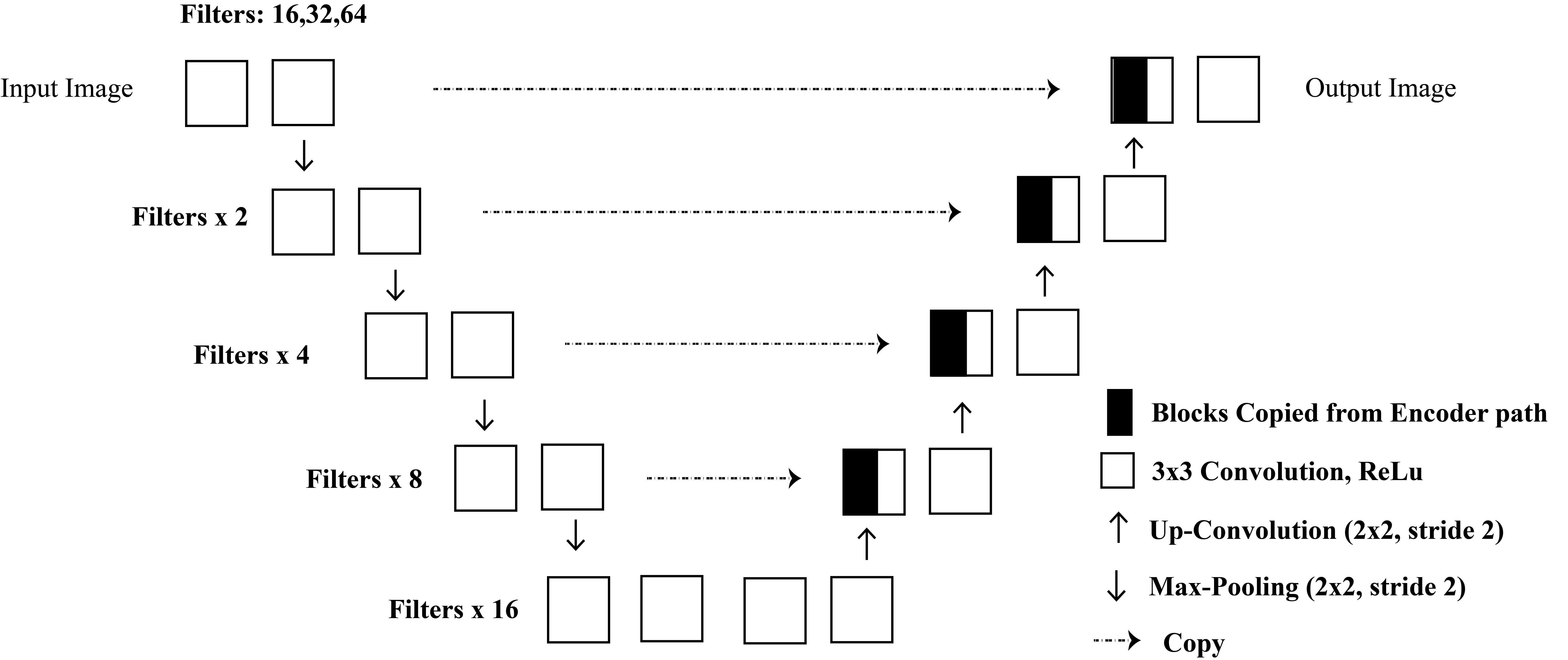
Figure 4: U-net architecture. Filters increase by 2ⁿ in each convolutional block.

3.2.2 Hyperparameters

The models were trained for 200 epochs with a fixed learning rate of 0.001. The initial tests also evaluated 0.01 and 0.0001 learning rate values, but the model’s accuracy was lower than the models trained with a learning rate of 0.001. Binary cross-entropy and Adam were used as the loss and optimization function, respectively. The models were trained with four different batch sizes (16, 32, 64, 128 samples). The model’s weights were just saved when the validation loss function decrease to reduce the overfitting.

The models were trained on Google Colaboratory virtual environment (Google, 2018) with Keras (Chollet et al., 2015) and Tensorflow (Abadi et al., 2015) Python libraries. 30% of each dataset was used as validation data.

3.3 Evaluation Metrics

The model’s performance was evaluated over two test areas by using f1-score, recall, precision, and mean intersect over union (mIoU) metrics. Those metrics are based on true positives (TP), false positives (FP), and false negatives (FN). TP are pixels correctly classified as landslides. FP represents the pixels incorrectly classified as landslides, and FN the pixels incorrectly classified as the background (Ghorbanzadeh et al., 2019, 2018; Guirado et al., 2017). The models that were trained with DEM as an additional channel were evaluated on test areas with an additional DEM channel.

3.3.1 Precision

Precision (Eq. 1) defines how accurate the model is by evaluating how much of the classified areas are landslides. The metric is useful for evaluating the cost of false positives.

$$Precision=\frac{True\>Positives}{True\>Positives+False\>Positives}$$ (1)

3.3.2 Recall

Recall (Eq. 2) calculates how many of the actual positives are true positives. This metric is suitable to evaluate the cost associated with false negatives.

$$Recal=\frac{True\>Positives}{True\>Positives+False\>Negatives}$$ (2)

3.3.3 F1-Score

F1-score (Eq. 3) combines precision and recall to measure if there is a balance between true positives and false negatives.

$$F1-Score=2*\frac{Precision\>*\>Recall}{Precision+Recall}$$ (3)

3.3.4 Mean Intersect Over Union (mIoU)

Mean intersect over union (Eq. 4), also known as Jaccard Index, computes the overlapping of areas between the ground truth (A) and the model prediction (B) divided by the union of these areas. Then, the values are averaged for each class. A value of 1 (one) represents perfect overlapping, while 0 (zero) represents no overlap.

$$mIoU=\frac{A\cap B}{A\cup B}=\frac{True\>Positives}{True\>Positives+False\>Positives+False\>Negatives}$$ (4)

The result section shows for each dataset, sampling method, and patch size the models with the highest F1-Score and mIoU. The complete results are available in the Supplementary Material. The model generalization was evaluated by averaging the mIoU values from both test areas.

4 Results and Discussion

The models were evaluated on two test areas with precision, recall, f1-score, and mIoU metrics. The results (Fig. 5) shows that the models trained with the RapidEye+DEM and RapidEye+DEM+Augmentation datasets achieved the best results in all evaluated metrics in test area one. The models trained with 32x32 tiles had the lowest precision (0.24) over all the datasets, while models trained with regular 64x64 and random 128x128 tiles from the RapidEye+DEM dataset achieved 0.67 and 0.66 of precision. The recall was higher for the models trained with 128x128 regular tiles (0.68) and 32x32 random tiles (0.65). The model trained with 128x128 random tiles from the RapidEye+DEM+Augmentation dataset achieved the best f1-score (0.55) and mIoU (0.38).

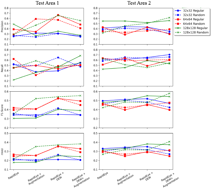
Figure 5: Precision, recall, f1-score and mIoU of the models with the highest f1-score and mIoU in test areas one (left) and two (right).

In test area two, the dataset had a smaller influence over the results; however, models trained with RapidEye+DEM+ +Augmentation dataset also achieved the best results. The model trained with 128x128 random tiles achieved the highest precision (0.62), f1-score (0.58), and mIoU (0.41). Just recall was higher for the 32x32 regular tiles (0.70).

Precision evaluates the cost of false positives, while recall evaluates the cost of false negatives. At test area one (Fig. 6, left), the 32x32 models had lower precision meaning that they misclassify more background areas as landslides (false positives). Similar results occur at test area two (Fig. 6, right), but 64x64 models also had low precision values. Recall varied among the datasets; nevertheless, in both test areas, the models trained with 32x32 tiles achieved high results. Therefore, these models classified more landslide areas as landslides (true positive), reducing false negatives.

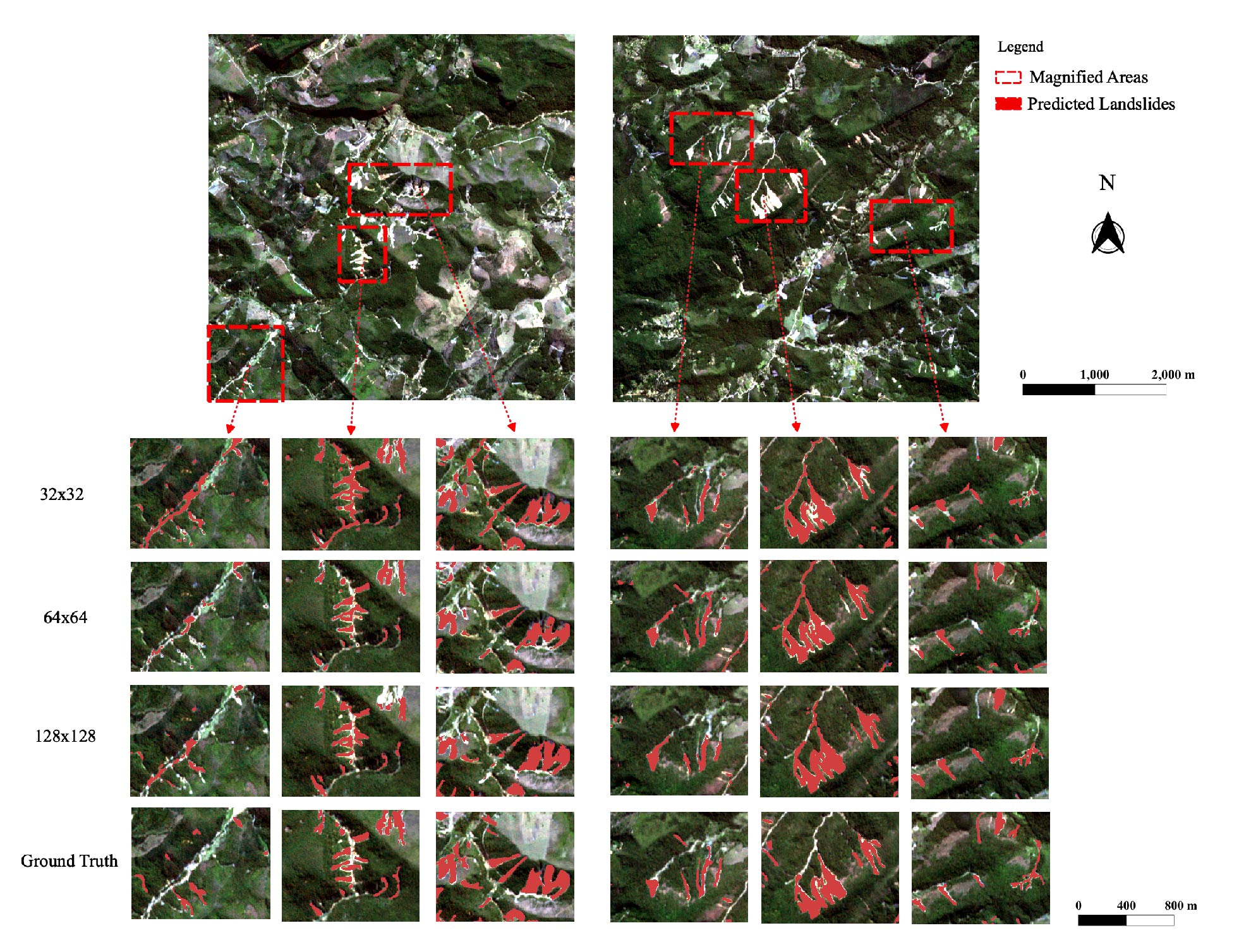
Figure 6: Results of the models with the highest mIoU on each test area. In test area one (left), the image shows the models trained with 32x32 and 64x64 regular tiles from the RapidEye+DEM dataset, and 128x128 random tiles from the RapidEye+DEM+Augmentation dataset. In test are two (right), the image shows the models trained 32x32 and 64x64 regular tiles from RapidEye+DEM dataset, and the 128x128 model trained with random tiles from the RapidEye+DEM+Augmentation dataset.

The F1-score value will always show a positive correlation with mIoU; however, mIoU tends to penalize incorrect classifications more quantitatively than f1-score. In both test areas, the models trained with random 128x128 tiles from the RapidEye+DEM+Augmentation dataset had the best f1-score and mIoU. In the test area one, this model achieved 0.55 of f1-score and 0.38 of mIoU. While in test area two, it achieved an f1-score of 0.58 and mIoU of 0.41. Comparing with the RapidEye dataset, where these models had the worst performance, the f1-score and mIoU increased 0.2 and 0.16 in test area one, and 0.16, 0.14 in test area two.

When the test areas are evaluated individually, the sampling method seems to be less critical than the dataset to the overall accuracy of the models. However, by averaging the mIoU score of both test areas, it can be seen (Table 3) that random sampling outperformed the regular sampling. Thus, random sampling helped in increasing the generalization capacity of the models. Moreover, similar to what was observed in each test area individually, models trained with DEM and DEM+Augmentation had a better performance.

Table 3: Results of the models with the highest average mIoU.

Sampling	Size	Test Area 1 - mIoU	Test Area 2 - mIoU	Average mIoU	Dataset
Random	32	0.26	0.32	0.29	RapidEye+DEM
Random	64	0.29	0.31	0.30	RapidEye+DEM+Augmentation
Random	128	0.31	0.41	0.36	RapidEye+DEM+Augmentation

The results (Fig. 7) of each model from table 3, shows that the 32x32 model predicted, in both test areas, 0.36 and 0.38 km² of true positives, 0.82 and 0.59 km² of false positives, achieving the highest values. While the model trained with 128x128 tiles predicted the smallest true positive areas (0.26 and 0.32 km²), false positive areas (0.29 and 0.20 km²), and larger false negatives (0.30 and 0.27 km²) and true negatives (25.37 and 25.42  m²) areas. The model trained with 64x64 tiles achieved values in between those two models, with 0.29 and 0.36 km² of true positives; 0.46, 0.57 km² of false positives; 0.27 and 0.23 km² of false negatives, and true negative of 25.19 and 25.05 km².

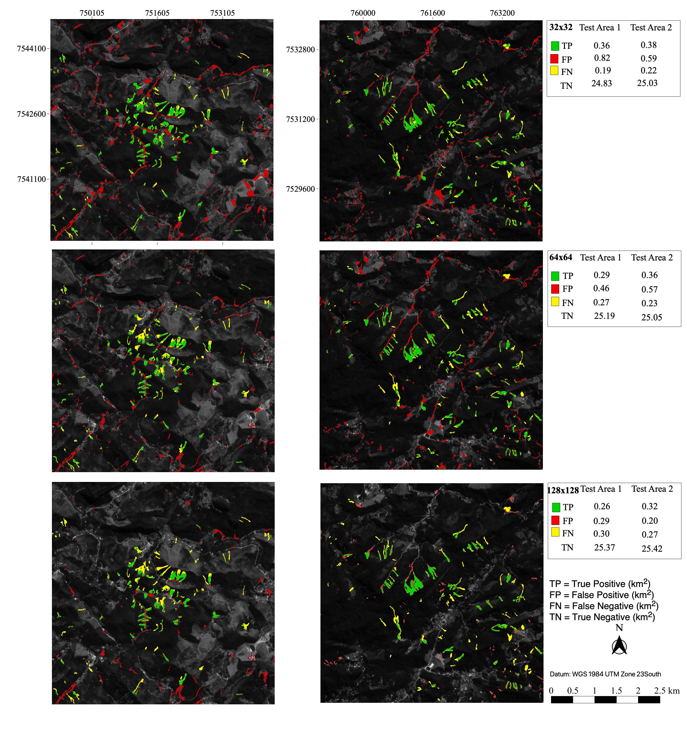
Figure 7: Results of the models with the best generalization results (Table 3), for each patch size, on test area one (left) and two (right).

The results of all evaluated models suggest that the models trained with smaller window sizes tend to understand the local context better. Thus, they classify more landslides correctly, achieving higher true positives and lower false negative values. However, as they are trained with small tiles, the scene’s global context, which helps differentiate the background areas, is lost. As a result, they misclassify more background areas as landslides (false positives). On the other hand, models trained with the larger window sizes, in general, understand the global context better, reducing the false positive errors. Nevertheless, they classify a smaller number of pixels representing landslide scars correctly, increasing the number of false negatives.

Areas with similar spectral responses to landslides such as rivers with increased bedload, gravel roads, grazing, and agricultural areas are more common in area one than area two. Therefore, the models usually make more false positives errors in this area. In area two, the most common false positive mistakes were due to human settlements.

5 Conclusions

This study’s main objective was to assess how the datasets, sampling methods, and patch sizes impact the overall performance of U-net on landslide segmentation. Our study suggests that the use of DEM and augmentation helped increase the overall accuracy of the models. Random sampling helped in increasing model generalization. Models trained with 32x32 patches classified more landslides areas correctly, thus, achieving higher true positive areas and lower false negatives. However, they also predict more false positive areas directly impacting precision, f1-score, and mIoU values. Contrarily, models trained with 128x128 tiles make less false positive errors and predict more areas correctly as background. Nevertheless, they also misclassify more landslide areas, increasing the number of false negatives and reducing the recall value. 64x64 tile models achieved results that lie in between the 32x32 and 128x128 models.

In our study, the use of the digital elevation model as an additional channel helped improve the accuracy of the models. This results differs from the ones obtained by Sameen and Pradhan (2019) and Ghorbanzadeh et al. (2019). However, since both authors used DEMs with higher spatial resolutions and the models were trained with different architectures and smaller tiles than the ones used in this research, more study is needed to address the most effective ways to use DEM with deep learning models. The 128x128 random model trained with the RapidEye+DEM+Augmentation dataset achieved the best performance in this research. The F1-score, 0.55 and 0.58, achieved in both test areas, is comparable to U-Net + ResNet34 evaluated by Prakash et al. (2020), which achieved 0.56 of f1-score, and the PspNet tested by Yu et al. (2020) that achieved f1-score of 0.6. Future studies should explore multi-input models that can be trained with different input sizes; and evaluate different post-processing segmentation techniques to increase the quality of the results.

Computer Code Availability

All the codes used in this research are available on GitHub: https://github.com/lpsmlgeobr/Landslide_segmentation_with_unet.

Data Availability

The RapidEye image used in this study (Image ID:2328825) was acquired from Planet (www.planet.com) through Planet’s Education and Research Program. The ALOS PALSAR DEM (Tile 26708) is available from the Alaska Satellite Facility (ASF) Distributed Active Archive Center (DAAC – https://search.asf.alaska.edu/).

References

- Kobiyama et al. [2006] Masato Kobiyama, Magaly Mendonça, Davis Anderson Moreno, IPVO Marcelino, Emerson V Marcelino, Edison F Gonçalves, Leticia LP Brazetti, Roberto F Goerl, Gustavo SF Molleri, and F de M Rudorff. Prevenção de desastres naturais: conceitos básicos. Organic Trading Curitiba, 2006.
- Hong et al. [2017] Haoyuan Hong, Wei Chen, Chong Xu, Ahmed M Youssef, Biswajeet Pradhan, and Dieu Tien Bui. Rainfall-induced landslide susceptibility assessment at the chongren area (china) using frequency ratio, certainty factor, and index of entropy. Geocarto international, 32(2):139–154, 2017.
- Alexander [2008] David E Alexander. A brief survey of gis in mass-movement studies, with reflections on theory and methods. Geomorphology, 94(3-4):261–267, 2008.
- Zhong et al. [2019] Cheng Zhong, Yue Liu, Peng Gao, Wenlong Chen, Hui Li, Yong Hou, Tuohuti Nuremanguli, and Haijian Ma. Landslide mapping with remote sensing: challenges and opportunities. International Journal of Remote Sensing, pages 1–27, 2019.
- UNISDR [2015] UNO UNISDR. Sendai framework for disaster risk reduction 2015–2030. In Proceedings of the 3rd United Nations World Conference on DRR, Sendai, Japan, pages 14–18, 2015.
- Mondini et al. [2019] Alessandro C Mondini, Michele Santangelo, Margherita Rocchetti, Enrica Rossetto, Andrea Manconi, and Oriol Monserrat. Sentinel-1 sar amplitude imagery for rapid landslide detection. Remote Sensing, 11(7):760, 2019.
- Guzzetti et al. [2012] Fausto Guzzetti, Alessandro Cesare Mondini, Mauro Cardinali, Federica Fiorucci, Michele Santangelo, and Kang-Tsung Chang. Landslide inventory maps: New tools for an old problem. Earth-Science Reviews, 112(1-2):42–66, 2012.
- Van Westen et al. [2008] Cees J Van Westen, Enrique Castellanos, and Sekhar L Kuriakose. Spatial data for landslide susceptibility, hazard, and vulnerability assessment: an overview. Engineering geology, 102(3-4):112–131, 2008.
- Zhong et al. [2020] Cheng Zhong, Yue Liu, Peng Gao, Wenlong Chen, Hui Li, Yong Hou, Tuohuti Nuremanguli, and Haijian Ma. Landslide mapping with remote sensing: challenges and opportunities. International Journal of Remote Sensing, 41(4):1555–1581, 2020.
- Xu [2015] Chong Xu. Preparation of earthquake-triggered landslide inventory maps using remote sensing and gis technologies: Principles and case studies. Geoscience Frontiers, 6(6):825–836, 2015.
- Yu et al. [2020] Bo Yu, Fang Chen, and Chong Xu. Landslide detection based on contour-based deep learning framework in case of national scale of nepal in 2015. Computers & Geosciences, 135:104388, 2020.
- Blaschke [2010] Thomas Blaschke. Object based image analysis for remote sensing. ISPRS journal of photogrammetry and remote sensing, 65(1):2–16, 2010.
- Stumpf and Kerle [2011] André Stumpf and Norman Kerle. Object-oriented mapping of landslides using random forests. Remote sensing of environment, 115(10):2564–2577, 2011.
- Blaschke et al. [2014] Thomas Blaschke, Geoffrey J Hay, Maggi Kelly, Stefan Lang, Peter Hofmann, Elisabeth Addink, Raul Queiroz Feitosa, Freek Van der Meer, Harald Van der Werff, Frieke Van Coillie, et al. Geographic object-based image analysis–towards a new paradigm. ISPRS journal of photogrammetry and remote sensing, 87:180–191, 2014.
- Prakash et al. [2020] Nikhil Prakash, Andrea Manconi, and Simon Loew. Mapping landslides on eo data: Performance of deep learning models vs. traditional machine learning models. Remote Sensing, 12(3):346, 2020.
- Ghorbanzadeh et al. [2019] Omid Ghorbanzadeh, Thomas Blaschke, Khalil Gholamnia, Sansar Raj Meena, Dirk Tiede, and Jagannath Aryal. Evaluation of different machine learning methods and deep-learning convolutional neural networks for landslide detection. Remote Sensing, 11(2):196, 2019.
- Peng et al. [2019] Daifeng Peng, Yongjun Zhang, and Haiyan Guan. End-to-end change detection for high resolution satellite images using improved unet++. Remote Sensing, 11(11):1382, 2019.
- Zhu et al. [2017] Xiao Xiang Zhu, Devis Tuia, Lichao Mou, Gui-Song Xia, Liangpei Zhang, Feng Xu, and Friedrich Fraundorfer. Deep learning in remote sensing: A comprehensive review and list of resources. IEEE Geoscience and Remote Sensing Magazine, 5(4):8–36, 2017.
- Long et al. [2015] Jonathan Long, Evan Shelhamer, and Trevor Darrell. Fully convolutional networks for semantic segmentation. In Proceedings of the IEEE conference on computer vision and pattern recognition, pages 3431–3440, 2015.
- Radovic et al. [2017] Matija Radovic, Offei Adarkwa, and Qiaosong Wang. Object recognition in aerial images using convolutional neural networks. Journal of Imaging, 3(2):21, 2017.
- Ding et al. [2016] Anzi Ding, Qingyong Zhang, Xinmin Zhou, and Bicheng Dai. Automatic recognition of landslide based on cnn and texture change detection. In 2016 31st Youth Academic Annual Conference of Chinese Association of Automation (YAC), pages 444–448. IEEE, 2016.
- Chen et al. [2018] Zhong Chen, Yifei Zhang, Chao Ouyang, Feng Zhang, and Jie Ma. Automated landslides detection for mountain cities using multi-temporal remote sensing imagery. Sensors, 18(3):821, 2018.
- Sameen and Pradhan [2019] Maher Ibrahim Sameen and Biswajeet Pradhan. Landslide detection using residual networks and the fusion of spectral and topographic information. IEEE Access, 7:114363–114373, 2019.
- Pradhan et al. [2017] Biswajeet Pradhan, Maher Ibrahim Seeni, and Haleh Nampak. Integration of lidar and quickbird data for automatic landslide detection using object-based analysis and random forests. In Laser Scanning Applications in Landslide Assessment, pages 69–81. Springer, 2017.
- Avelar et al. [2013] André S Avelar, Ana L Coelho Netto, Willy A Lacerda, Leonardo B Becker, and Marcos B Mendonça. Mechanisms of the recent catastrophic landslides in the mountainous range of rio de janeiro, brazil. In Landslide science and practice, pages 265–270. Springer, 2013.
- Dantas [2001] M. E. Dantas. Geomorfologia do estado do rio de janeiro. CPRM. Estudo geoambiental do Estado do Rio de Janeiro. Brasília, 2001.
- Tupinambá et al. [2012] Miguel Tupinambá, Monica Heilbron, Beatriz Paschoal Duarte, Julio Cesar Horta de Almeida, Claudia Sayão Valladares, Bruno Trota Pacheco, Marcelo dos Santos Salomão, Flávio Ribeiro Conceição, Luiz Guilherme Eirado da Silva, Clayton Guia de Almeida, Marcelo Ambrósio Ferrassoli, Mariana de Cássia O. da Costa, Luciana Rocha Tupinambá, David Silva Rocha, Pedro Monteiro Benac, Hugo Mathias O. Carvalho da Silva, Paulo Vicente Guimarães, (DRM-RJ), (DRM-RJ), Felipe de Lima da Silva, Nely Palermo, and Ronaldo Mello Pereira. Mapa geológico folha nova friburgo sf-23-z-b-ii. Technical report, CPRM - Serviço Geológico do Brasil, 2012.
- Köppen [1936] W. Köppen. Das geographische System der Klimate, volume 1, chapter Das geographische System der Klimate, pages 1–44. Gerbrüder Bornträger, 1936.
- Sobral et al. [2018] Bruno Serafini Sobral, José Francisco Oliveira-Júnior, Givanildo Gois, Paulo Miguel de Bodas Terassi, and João Gualberto Rodrigues Muniz-Júnior. Variabilidade espaço-temporal e interanual da chuva no estado do rio de janeiro. Revista Brasileira de Climatologia, 22, 2018.
- RapidEye [2011] AG RapidEye. Satellite imagery product specifications. Satellite imagery product specifications: Version, 2011.
- Planet Team [2017] Planet Team. Planet application program interface: In space for life on earth. san francisco, ca, 2017. Available online: https://api.planet.com. Last accessed on 2020-05-1.
- DAAC [2015] ASF DAAC. Alos palsar_radiometric_terrain_corrected_high_res. JAXA/METI, 11, 2015. https://search.asf.alaska.edu/#/, Last accessed on 2019-12-05.
- Neteler et al. [2012] Markus Neteler, M. Hamish Bowman, Martin Landa, and Markus Metz. GRASS GIS: A multi-purpose open source GIS. Environmental Modelling & Software, 31:124–130, 2012. ISSN 1364-8152. doi: 10.1016/j.envsoft.2011.11.014.
- GRASS Development Team [2017] GRASS Development Team. Geographic Resources Analysis Support System (GRASS GIS) Software, Version 7.2. Open Source Geospatial Foundation, 2017. URL http://grass.osgeo.org.
- QGIS Development Team [2009] QGIS Development Team. QGIS Geographic Information System. Open Source Geospatial Foundation, 2009. URL http://qgis.osgeo.org.
- Google [2019] Google. Google earth pro version 7.3, 2019. https://www.google.com/earth/versions/#download-pro, Last accessed on 2020-04-20.
- Netto et al. [2013] Ana Luiza Coelho Netto, Anderson Mululo Sato, André de Souza Avelar, Lílian Gabriela G Vianna, Ingrid S Araújo, David LC Ferreira, Pedro H Lima, Ana Paula A Silva, and Roberta P Silva. January 2011: the extreme landslide disaster in brazil. In Landslide science and practice, pages 377–384. Springer, 2013.
- Gillies et al. [2013–] Sean Gillies et al. Rasterio: geospatial raster i/o for Python programmers, 2013–. URL https://github.com/mapbox/rasterio.
- Oliphant [2006] Travis E Oliphant. A guide to NumPy, volume 1. Trelgol Publishing USA, 2006.
- Terstriep [2019] Jeff Terstriep. Keras spatial, 2019. https://pypi.org/project/keras-spatial/, Last accessed on 2020-02-10.
- Buslaev et al. [2018] A. Buslaev, A. Parinov, E. Khvedchenya, V. I. Iglovikov, and A. A. Kalinin. Albumentations: fast and flexible image augmentations. ArXiv e-prints, 2018.
- Ronneberger et al. [2015] Olaf Ronneberger, Philipp Fischer, and Thomas Brox. U-net: Convolutional networks for biomedical image segmentation. In International Conference on Medical image computing and computer-assisted intervention, pages 234–241. Springer, 2015.
- Google [2018] Google. Google colaboratory, 2018. https://colab.research.google.com/, Last accessed on 2020-05-12.
- Chollet et al. [2015] François Chollet et al. Keras. https://github.com/fchollet/keras, 2015.
- Abadi et al. [2015] Martín Abadi, Ashish Agarwal, Paul Barham, Eugene Brevdo, Zhifeng Chen, Craig Citro, Greg S. Corrado, Andy Davis, Jeffrey Dean, Matthieu Devin, Sanjay Ghemawat, Ian Goodfellow, Andrew Harp, Geoffrey Irving, Michael Isard, Yangqing Jia, Rafal Jozefowicz, Lukasz Kaiser, Manjunath Kudlur, Josh Levenberg, Dandelion Mané, Rajat Monga, Sherry Moore, Derek Murray, Chris Olah, Mike Schuster, Jonathon Shlens, Benoit Steiner, Ilya Sutskever, Kunal Talwar, Paul Tucker, Vincent Vanhoucke, Vijay Vasudevan, Fernanda Viégas, Oriol Vinyals, Pete Warden, Martin Wattenberg, Martin Wicke, Yuan Yu, and Xiaoqiang Zheng. TensorFlow: Large-scale machine learning on heterogeneous systems, 2015. URL https://www.tensorflow.org/. Software available from tensorflow.org.
- Ghorbanzadeh et al. [2018] Omid Ghorbanzadeh, Dirk Tiede, Zahra Dabiri, Martin Sudmanns, and Stefan Lang. Dwelling extraction in refugee camps using cnn–first experiences and lessons learnt. International Archives of the Photogrammetry, Remote Sensing & Spatial Information Sciences, 2018.
- Guirado et al. [2017] Emilio Guirado, Siham Tabik, Domingo Alcaraz-Segura, Javier Cabello, and Francisco Herrera. Deep-learning convolutional neural networks for scattered shrub detection with google earth imagery. arXiv preprint arXiv:1706.00917, 2017.