Expansion dynamics in two-dimensional Bose-Hubbard lattices:
Bose-Einstein condensate and thermal cloud

Abstract

We study the temporal expansion of an ultracold Bose gas in two-dimensional, square optical lattices. The gas is described by the Bose-Hubbard model deep in the superfluid regime, with initially all bosons condensed in the central site of the lattice. We use the previously developed nonequilibrium propagator method for capturing the time evolution of an interacting bosonic system, where the many-body Hamiltonian is represented in an appropriate local basis and the corresponding field operators are separated into the classical [Bose-Einstein condensate (BEC)] part and quantum mechanical fluctuations. After a quench, i.e., after a sudden switch of the lattice nearest-neighbor hopping, the expanding bosonic cloud separates spatially into a fast ballistic forerunner and a slowly expanding central part controlled by self-trapping. We show that the forerunner expansion is driven by the coherent dynamics of the BEC and that its velocity is consistent with the Lieb-Robinson bound. For smaller lattices we analyze how quasiparticle collisions lead to enhanced condensate depletion and oscillation damping.

I Introduction

The Bose-Hubbard model has been in the focus of condensed-matter research since the seminal paper by Fisher et al. Fisher1989 , which predicted a superfluid–Mott-localization transition, and especially after its experimental realization in ultracold-atom systems Greiner2002 . It is well known that systems of cold atoms encompass a number of impressive advantages over their solid-state counterparts, among which are the full system controllability, freedom from impurities, isolation from the environment, and the possibility to realize quantum quenches. A quantum quench, i.e., an abrupt change of one of the system’s parameters, is a controlled way to bring a system out of equilibrium Polkovnikov2011 ; Schmiedmayer2015 ; Eisert2015 and to study its nonequilibrium dynamics and potential thermalization Eisert2016 ; Rigol2016 .

The temporal expansion of clouds of interacting bosonic atoms in optical lattices has been studied experimentally Schneider2013 ; Reinhard2013 ; Weiss2015 ; Schneider2015 and theoretically Rigol2011 ; Rigol2013 ; Weiss2013 ; Heidrich-Meisner2013 ; Boschi2014 ; Heidrich-Meisner2015 ; Rigol2017 as a straightforward way of accessing the nonequilibrium dynamics of these systems. Most of these studies used a low-density, incoherent or Mott insulating initial state and investigated various aspects of the time evolution, such as self-trapping effects slowing down the expansion Reinhard2013 ; Rigol2013 ; Weiss2013 , a bimodal structure of the expanding cloud Schneider2013 ; Schneider2015 ; Rigol2011 ; Heidrich-Meisner2015 , and doublon dynamics Boschi2014 and the expulsion of single bosons in the halo of the cloud, termed the quantum distillation effect Weiss2015 . Specifically, in the experiment Schneider2013 a Mott insulating core with unity filling was prepared in the center of a two-dimensional (2D) optical lattice. By abruptly lowering the lattice depth in one or both directions, tunneling and correspondingly expansion of the boson gas was induced and studied in detail in dependence on the interaction strength $U$. It was found that both dimensionality and interaction play an important role in the nonequilibrium expansion dynamics. In particular, the expansion in a 2D lattice developed bimodal cloud shapes with slow dynamics in the round, central part of the cloud surrounded by fast, square-shaped ballistic wings. The core expansion velocity slowed down with the growth of interaction and eventually saturated Schneider2013 . On the theoretical side, expansion dynamics in more than one spatial dimension has so far been studied on the level of mean-field theories Rigol2011 ; Rigol2013 ; Shapiro2007 , that is, considering the dynamics of the Bose-Einstein condensate (BEC) and neglecting the influence of the thermal cloud or incoherent excitations. In particular, time-dependent Gutzwiller mean-field theory was employed to analyze the expansion dynamics in 2D bosonic Mott-Hubbard lattices Rigol2011 ; Rigol2013 ; Atav2014 . It was found that initially confined Mott-insulating states become coherent during the expansion after removal of a confining potential Rigol2011 , and initially superfluid states with small occupation numbers expand in a bimodal way with a central, slowly expanding cloud surrounded by a rapidly expanding low-density cloud of bosons Rigol2013 . The bosons expand ballistically and fastest along the diagonals of the lattice. In these works, the physics behind the expansion behavior was attributed to the fact, that the central cloud consists predominantly of doublons, which tend to group together Muth2012 , whereas the fast expanding part consists of monomers Rigol2013 ; Weiss2015 .

However, previous studies of the quench dynamics of Bose-Josephson junctions (BJJs) Mauro2009 ; Mauro2015 ; Anna2016 ; Annalen2018 ; Lappe2018 showed that incoherent fluctuations become inevitably excited after the quench even in gapped systems, due to the finite spectral distribution involved in the temporal evolution. The coupling of the BEC to these incoherent excitations plays an important role in the relaxation and thermalization dynamics Anna2016 ; Annalen2018 ; Lappe2018 . Exact numerical calculations of the expansion dynamics are possible only in one dimension Schneider2013 ; Kollath2012 , where true Bose-Einstein condensation does not occur and, hence, a sharp distinction between BEC and incoherent excitations is not possible in the time-dependent situation.

In the present article we investigate the regime of high initial density. In this regime, doublon dynamics will not play an important role, so the effect of interaction-induced self-trapping on the expansion dynamics can be studied independently. We also analyze the dynamics of the coherent BEC and of the noncondensed particle cloud separately and study the condensate depletion induced by the nonequilibrium dynamics. To tackle the problem of the expansion of the coupled system of BEC and incoherent fluctuations we therefore adopt the semianalytical formalism developed earlier and applied for studies of nonequilibrium BJJs Mauro2009 ; Anna2016 ; Annalen2018 . Our approach goes beyond mean-field approximations and systematically takes into account incoherent excitations. It consists of coupled equations of motion for the classical space-time-dependent BEC amplitudes and for the full Keldysh quantum propagators of the noncondensate fluctuations. These equations are derived from a generating functional using the Keldysh-Kadanoff-Baym nonequilibrium approach Kadanoffbook ; Sieberer2016 ; Annalen2018 , which leads to a hierarchy of conserving approximations, and are solved self-consistently. We focus on the expansion dynamics of weakly interacting bosons in two dimensions, deep in the superfluid phase. For large square lattices of size $21\times 21$, we evaluate the theory within the leading-order-in-$U$ conserving approximation, the Bogoliubov-Hartree-Fock (BHF) approximation, while for smaller system size ($3\times 3$) we use the second-order self-consistent approximation, thus taking inelastic relaxation processes into account. Unlike previous treatments Rigol2011 ; Rigol2013 we can consider arbitrary large numbers of particles within our formalism. Note, however, that we do not attain the Mott localized phase since the interactions are assumed to be weak.

As the main results we find that even for small interaction strength but large values of the initial local occupation number the coherent part of the expanding cloud splits into two modes, a slowly expanding high-density central part and a fast expanding low-density pulse or “forerunner.” In this case of high occupation number, however, the expansion of the high-density part is not inhibited by doublon formation Rigol2013 but by the interaction-induced self-trapping effect known from the oscillation dynamics of BJJs Smerzi1997 ; Albiez2005 ; Mauro2009 . The forerunner expands ballistically, typical for coherent waves, instead of diffusively. Despite the different initial conditions, these results are in good agreement with experiments on 2D expansion of low-density Bose gases Schneider2013 . The forerunner’s expansion speed is largest along the lattice diagonals where it obeys and reaches the Lieb-Robinson bound Lieb1972 . The latter states that there is a finite limit to the speed of information propagation in any quantum system.

In addition, we are able to distinguish the dynamics of the incoherent excitation cloud from the coherent one. The density of incoherent excitations increases with the interaction strength $U$, as expected, but with increasing $U$ it ceases to participate in the forerunner. This confirms that the forerunner is a coherence phenomenon. Taking inelastic two-particle scattering into account for small lattices beyond the BHF approximation, we find that it leads to fast damping of density oscillations between the BEC and the incoherent fluctuations and to enhanced depletion of the condensate.

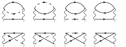
Figure 1: Diagrams contributing to the second-order self-energies. Indices $1$ and $1^{\prime}$ refer to the first and second arguments of the self-energies ($1\equiv{\bf r},t$ and $1^{\prime}\equiv{\bf r^{\prime}},t^{\prime}$). Solid lines represent propagators of noncondensed particles, whereas dashed lines denote propagators of condensed bosons. The wavy lines are associated with the interaction $U$.

This article is organized as follows. In Sec. II we describe our model and derive the general kinetic equations based on the Keldysh-Kadanoff-Baym nonequilibrium approach. Section II.2 contains the equations of motion without two-particle damping, i.e., the dynamical BHF approximation, while in Sec. II.3 the collision integrals describing inelastic interactions are taken into account. The results within the BHF approximation and including inelastic processes are presented and discussed in detail in Secs. III.1 and III.2, respectively. We summarize in Sec. IV.

II Model and equations of motion

II.1 General kinetic equations

We consider ultracold bosons in a 2D, square optical lattice described by the Bose-Hubbard Hamiltonian Jaksch1998

$$H=-J(t)\sum_{\langle i,j\rangle}\hat{b}^{\dagger}_{i}\hat{b}^{\phantom{\dagger}}_{j}+\sum_{i}\varepsilon_{i}\ \hat{b}^{\dagger}_{i}\hat{b}^{\phantom{\dagger}}_{i}+\frac{U}{2}\sum_{i}\hat{n}_{i}(\hat{n}_{i}-1),$$ (1)

where $U$ is the repulsive interaction between bosons, and $J(t)=J\Theta(t)$ is the nearest neighbor hopping amplitude which is abruptly switched on at time $t=0$, with $\Theta(t)$ the Heaviside Theta function. In addition, $\hat{b}^{\dagger}_{i}$ and $\hat{b}_{i}$ are bosonic creation and annihilation operators on site $i$, respectively, and $\hat{n}_{i}=\hat{b}^{\dagger}_{i}\hat{b}^{\phantom{\dagger}}_{i}$ is the boson number operator. Hereafter we will consider a homogeneous lattice, $\varepsilon=\varepsilon_{i}$ for any $i$. As initial conditions at $t=0$ we assume all bosons condensed deep in the superfluid phase and trapped by a tight confining potential in the central site of the lattice.

After the tunneling $J(t)$ is turned on for $t>0$, two main processes set in: (i) the superfluid part is allowed to expand in all directions of the lattice and (ii) incoherent excitations get excited and are expanding along with the superfluid part. We analyze the resultant dynamics using the formalism developed earlier Mauro2009 ; Mauro2015 based on standard nonequilibrium techniques Kadanoffbook ; Griffinbook ; Rammerbook . As usual, we decompose the bosonic operators into their expectation or saddlepoint value $a_{i}(t)=\langle\hat{b}_{i}\rangle$ and the fluctuations $\hat{\varphi}_{i}$,

$$\hat{b}_{i}=a_{i}(t)+\hat{\varphi}_{i},\quad\hat{b}_{i}^{\dagger}=a_{i}^{*}(t)+\hat{\varphi}_{i}^{\dagger},$$ (2)

where $a_{i}(t)$ represents the local BEC amplitude and the noncondensate quantum fluctuations are described by the operators $\hat{\varphi}_{i}=\hat{b}_{i}-a_{i}(t)$ obeying canonical bosonic commutation relations. We now treat the condensate amplitudes semiclassically and the quantum fluctuations quantum field theoretically in order to capture the nonequilibrium dynamics. The full bosonic propagator splits into two parts ${\bf C}+{\bf G}$, with

$${\bf C}_{ij}(t,t^{\prime}) = -{i}\left(\begin{matrix}a_{i}(t)a_{j}^{*}(t^{\prime})&a_{i}(t)a_{j}(t^{\prime})\\ a_{i}^{*}(t)a_{j}^{*}(t^{\prime})&a_{i}^{*}(t)a_{j}(t^{\prime})\end{matrix}\right),$$ (3)

$${\bf G}_{ij}(t,t^{\prime}) = -{i}\left(\begin{matrix}\langle T_{C}\hat{\varphi}_{i}(t)\hat{\varphi}_{j}^{\dagger}(t^{\prime})\rangle&\langle T_{C}\hat{\varphi}_{i}(t)\hat{\varphi}_{j}(t^{\prime})\rangle\\ \langle T_{C}\hat{\varphi}_{i}^{\dagger}(t)\hat{\varphi}_{j}^{\dagger}(t^{\prime})\rangle&\langle T_{C}\hat{\varphi}_{i}^{\dagger}(t)\hat{\varphi}_{j}(t^{\prime})\rangle\end{matrix}\right)=\left(\begin{matrix}G_{ij}(t,t^{\prime})&F_{ij}(t,t^{\prime})\\ \overline{F}_{ij}(t,t^{\prime})&\overline{G}_{ij}(t,t^{\prime})\end{matrix}\right),$$ (4)

where $T_{C}$ denotes time-ordering operator along the Keldysh contour and ${i}$ the imaginary unit. The general Dyson equations for the propagators ${\bf C}$ and ${\bf G}$ read

$$\sum_{k}\int\limits_{C}d\overline{t}\left[{\bf G}_{0,ik}^{-1}(t,\overline{t})-{\bf S}^{HF}_{ik}(t,\overline{t})\right]{\bf C}_{kj}(\overline{t},t^{\prime}) = \sum_{k}\int\limits_{C}d\overline{t}{\bf S}_{ik}(t,\overline{t}){\bf C}_{kj}(\overline{t},t^{\prime}),$$ (5)

$$\sum_{k}\int\limits_{C}d\overline{t}\left[{\bf G}_{0,ik}^{-1}(t,\overline{t})-{\bf\Sigma}^{HF}_{ik}(t,\overline{t})\right]{\bf G}_{kj}(\overline{t},t^{\prime}) = \mathds{1}\delta(t-t^{\prime})\delta_{ij}+\sum_{k}\int\limits_{C}d\overline{t}{\bf\Sigma}_{ik}(t,\overline{t}){\bf G}_{kj}(\overline{t},t^{\prime}).$$ (6)

Here all integrals as well as the Dirac $\delta(t-t^{\prime})$ are defined along the Keldysh contour $C$. For convenience, we also separate the selfenergy into two parts: the local Hartree-Fock (HF) part and the collision part, described by ${\bf S}$ and ${\bf\Sigma}$, respectively Mauro2015 ; Annalen2018 . The inverse bare propagator reads

$${\bf G}^{-1}_{0,ij}(t,t^{\prime})=\left[{i}\,{\bf\bm{\tau}}_{3}\,\delta_{ij}\frac{\partial}{\partial t}+J\,\mathds{1}\,\delta_{\langle i,j\rangle}\right]\delta(t-t^{\prime}),$$ (7)

where $\mathds{1}$ and $\bm{\tau}_{3}$ denote the unit and the third Pauli matrix in Bogoliubov particle-hole space, respectively. In addition, $\delta_{\langle i,j\rangle}$ is $1$ if $i$ and $j$ are nearest neighbors and zero otherwise. For further analysis it is convenient to rewrite the general Dyson equations (5) and (6) in terms of symmetrized and antisymmetrized field-correlation functions

$${\bf A}_{ij}(t,t^{\prime}) = {i}\left[{\bf G}_{ij}^{>}(t,t^{\prime})-{\bf G}_{ij}^{<}(t,t^{\prime})\right]=\begin{pmatrix}\text{A}_{ij}^{G}&\text{A}_{ij}^{F}\\ \text{A}_{ij}^{\overline{F}}&\text{A}_{ij}^{\overline{G}}\end{pmatrix},$$

$${\bf F}_{ij}(t,t^{\prime}) = \frac{1}{2}\left[{\bf G}_{ij}^{>}(t,t^{\prime})+{\bf G}_{ij}^{<}(t,t^{\prime})\right]=\begin{pmatrix}\text{F}_{ij}^{G}&\text{F}_{ij}^{F}\\ \text{F}_{ij}^{\overline{F}}&\text{F}_{ij}^{\overline{G}}\end{pmatrix},$$

where we omitted the time arguments in the matrix representations for simplicity. Similarly, we introduce, for the self-energies,

$${\bm{\gamma}}_{ij}(t,t^{\prime}) = {i}\left[{\bf S}_{ij}^{>}(t,t^{\prime})-{\bf S}_{ij}^{<}(t,t^{\prime})\right]=\begin{pmatrix}\gamma_{ij}^{G}&\gamma_{ij}^{F}\\ \gamma_{ij}^{\overline{F}}&\gamma_{ij}^{\overline{G}}\end{pmatrix},$$

$${\bf\Gamma}_{ij}(t,t^{\prime}) = {i}\left[{\bf\Sigma}_{ij}^{>}(t,t^{\prime})-{\bf\Sigma}_{ij}^{<}(t,t^{\prime})\right]=\begin{pmatrix}\Gamma_{ij}^{G}&\Gamma_{ij}^{F}\\ \Gamma_{ij}^{\overline{F}}&\Gamma_{ij}^{\overline{G}}\end{pmatrix},$$

$${\bf\Pi}_{ij}(t,t^{\prime}) = \frac{1}{2}\left[{\bf\Sigma}_{ij}^{>}(t,t^{\prime})+{\bf\Sigma}_{ij}^{<}(t,t^{\prime})\right]=\begin{pmatrix}\Pi_{ij}^{G}&\Pi_{ij}^{F}\\ \Pi_{ij}^{\overline{F}}&\Pi_{ij}^{\overline{G}}\end{pmatrix}.$$

The symbols $<$ and $>$ refer to the standard lesser and greater notations for nonequilibrium Green’s functions and self-energies Rammerbook .

With this new notation we can rewrite Eqs. (5) and (6) in terms of symmetrized and antisymmetrized correlators and their selfenergies

$${i}\bm{\tau}_{3}\frac{\partial}{\partial t}{\bf C}_{ij} = -J(\sum_{i^{\prime}:\langle i^{\prime},i\rangle}{\bf C}_{i^{\prime},j}+\sum_{j^{\prime}:\langle j^{\prime},j\rangle}{\bf C}_{i,j^{\prime}})+{\bf S}_{i}^{HF}{\bf C}_{ij}-{i}\sum_{k}\int\limits_{0}^{t}d\overline{t}{\bm{\gamma}}_{ik}{\bf C}_{kj},$$ (10)

$${i}\bm{\tau}_{3}\frac{\partial}{\partial t}{\bf A}_{ij} = -J(\sum_{i^{\prime}:\langle i^{\prime},i\rangle}{\bf A}_{i^{\prime},j}+\sum_{j^{\prime}:\langle j^{\prime},j\rangle}{\bf A}_{i,j^{\prime}})+{\bf\Sigma}_{i}^{HF}{\bf A}_{ij}-{i}\sum_{k}\int\limits_{t^{\prime}}^{t}d\overline{t}{\bf\Gamma}_{ik}{\bf A}_{kj},$$ (11)

$${i}\bm{\tau}_{3}\frac{\partial}{\partial t}{\bf F}_{ij} = -J(\sum_{i^{\prime}:\langle i^{\prime},i\rangle}{\bf F}_{i^{\prime},j}+\sum_{j^{\prime}:\langle j^{\prime},j\rangle}{\bf F}_{i,j^{\prime}})+{\bf\Sigma}_{i}^{HF}{\bf F}_{ij}-\ {i}\sum_{k}\int\limits_{0}^{t}d\overline{t}{\bf\Gamma}_{ik}{\bf F}_{kj}+{i}\sum_{k}\int\limits_{0}^{t^{\prime}}d\overline{t}{\bf\Pi}_{ik}{\bf A}_{kj}.$$ (12)

In Eqs. (11) and (12) we used the locality of the Hartree-Fock selfenergies in the time arguments as well as in the site indices, i.e., ${\bf S}_{ij}^{HF}={\bf S}_{i}^{HF}\delta_{ij}\delta(t-t^{\prime})$ and similarly for ${\bf\Sigma}^{HF}_{ij}$, and evaluated the contour integrals. Here and in the following, a sum index $i^{\prime}:\langle i^{\prime},i\rangle$ indicates summation of $i^{\prime}$ over nearest neighbors of fixed $i$. Because of the quench boundary conditions, the integrals involving collisional self-energies in Eqs. (10)–(12) start from $0$ and not from $-\infty$. For simplicity, we omitted again explicit time arguments of the Green’s functions and self-energies. The argument $t$ refers to the first argument of the functions and selfenergies, that is, ${\bf C}_{ij}\equiv{\bf C}_{ij}(t,t^{\prime})$ and $\int\limits_{t^{\prime}}^{t}d\overline{t}\,{\bf\Gamma}_{ik}{\bf A}_{kj}=\int\limits_{t^{\prime}}^{t}d\overline{t}\,{\bf\Gamma}_{ik}(t,\overline{t}){\bf A}_{kj}(\overline{t},t^{\prime})$, etc. The boundary conditions are formulated in such a way that the system of equations (10)–(12) becomes an initial value problem.

II.2 Bogoliubov-Hartree-Fock approximation

In this section we specify the set of differential equations derived from (10)–(12) in the BHF approximation, i.e., the first-order-in-$U$ conserving approximation Griffinbook . To first order in $U$ we neglect the integrals in Eqs. (10)–(12) and explicitly calculate the HF self-energies ${\bf S}^{HF}$ and ${\bf\Sigma}^{HF}$ as

$${\bf\Sigma}_{i}^{HF} = \begin{pmatrix}\Sigma_{i}^{HF}&\Omega_{i}^{HF}\\ \overline{\Omega}_{i}^{HF}&\overline{\Sigma}_{i}^{HF}\end{pmatrix}={i}U\left[\left(\frac{1}{2}\text{Tr}[{\bf C}_{ii}]\mathds{1}+{\bf C}_{ii}\right)+\left(\frac{1}{2}\text{Tr}[{\bf F}_{ii}]\mathds{1}+{\bf F}_{ii}\right)\right],$$ (13)

$${\bf S}_{i}^{HF} = \begin{pmatrix}S_{i}^{HF}&W_{i}^{HF}\\ \overline{W}_{i}^{HF}&\overline{S}_{i}^{HF}\end{pmatrix}={i}U\left[\frac{1}{2}\text{Tr}[{\bf C}_{ii}]\mathds{1}+\left(\frac{1}{2}\text{Tr}[{\bf F}_{ii}]\mathds{1}+{\bf F}_{ii}\right)\right].$$ (14)

Note that, in this approximation, quantities related to the spectral function ${\bf A}_{ij}$ decouple from the system of equations, and the final system of BHF equations reads

$${i}\frac{\partial}{\partial t}a_{i}=-J\sum_{i^{\prime}:\langle i^{\prime},i\rangle}a_{i^{\prime}}+(U|a_{i}|^{2}+2{i}U\text{F}_{ii}^{G})a_{i}+{i}U\text{F}_{ii}^{F}a_{i}^{*},$$ (15)

$${i}\frac{\partial}{\partial t}\text{F}^{G}_{ij}=-J\Bigl{(}\sum_{i^{\prime}:\langle i^{\prime},i\rangle}\text{F}^{G}_{i^{\prime},j}+\sum_{j^{\prime}:\langle j^{\prime},j\rangle}\text{F}^{G}_{i,j^{\prime}}\Bigr{)}+\Sigma_{i}^{HF}\text{F}^{F}_{ij}-\text{F}^{F}_{ij}\Sigma_{j}^{HF}-\Omega_{i}^{HF}(\text{F}^{F}_{ij})^{*}-\text{F}^{F}_{ij}(\Omega_{j}^{HF})^{*},$$

$${i}\frac{\partial}{\partial t}\text{F}^{F}_{ij}=-J\Bigl{(}\sum_{i^{\prime}:\langle i^{\prime},i\rangle}\text{F}^{F}_{i^{\prime},j}+\sum_{j^{\prime}:\langle j^{\prime},j\rangle}\text{F}^{F}_{i,j^{\prime}}\Bigr{)}+\Sigma_{i}^{HF}\text{F}^{F}_{ij}+\text{F}^{F}_{ij}\Sigma_{j}^{HF}-\Omega_{i}^{HF}(\text{F}^{G}_{ij})^{*}-\text{F}^{G}_{ij}\Omega_{j}^{HF}.$$

We then solve the equations numerically, the results being discussed in detail in section III.1.

II.3 Selfconsistent second-order approximation

In the self-consistent second-order approximation, accounting for collisions and relaxation, the equations are significantly more complicate, and the spectral and statistical parts are coupled, unlike in the BHF approximation. The diagrammatic contributions to the self-energies in second order are depicted in Fig. 1. Due to the underlying symmetry relations specified in Appendix A, we give here only the expressions for the upper-left and upper-right components of the second-order matrix self-energy ${\bm{\gamma}_{ij}}$ [see Eqs. (10)–(12)],

$$\gamma^{G}_{ij} = U^{2}\text{F}^{G}_{ij}(4\Lambda_{ij}[F,F^{*}]+2\Lambda_{ij}[G,G^{*}])+U^{2}\text{A}^{G}_{ij}(4\Xi_{ij}[F,F^{*}]+2\Xi_{ij}[G,G^{*}]),$$ (16)

$$\gamma^{F}_{ij} = U^{2}\text{F}^{F}_{ij}(4\Lambda_{ij}[G,G^{*}]+2\Lambda_{ij}[F,F^{*}])+U^{2}\text{A}^{F}_{ij}(4\Xi_{ij}[G,G^{*}]+2\Xi_{ij}[F,F^{*}]).$$ (17)

Here we introduced the shorthand notation

$$\Lambda_{ij}[f,g](t,t^{\prime}) = \text{A}_{ij}^{f}(t,t^{\prime})\text{F}_{ij}^{g}(t,t^{\prime})+\text{A}_{ij}^{g}(t,t^{\prime})\text{F}_{ij}^{f}(t,t^{\prime}),$$

$$\Xi_{ij}[f,g](t,t^{\prime}) = \text{F}_{ij}^{f}(t,t^{\prime})\text{F}_{ij}^{g}(t,t^{\prime})-\frac{1}{4}\text{A}_{ij}^{f}(t,t^{\prime})\text{A}_{ij}^{g}(t,t^{\prime}),$$

where $g,f\in\{G,F,G^{*},F^{*}\}$ and $A^{g^{*}}\equiv(A^{g})^{*}$. The other two contributions ${\bf\Gamma}_{ij}$ and ${\bf\Pi}_{ij}$ from Eqs. (10)–(12) are expressed as

$$\Gamma_{ij}^{G}=2{i}U^{2}(2a_{i}^{*}a_{j}^{*}\Lambda_{ij}[F,G]+a_{i}^{*}a_{j}\Lambda_{ij}[G,G]-2a_{i}a_{j}\Lambda_{ij}[F^{*},G]-2a_{i}a_{j}^{*}\Lambda_{ij}[G,G^{*}]-2a_{i}a_{j}^{*}\Lambda_{ij}[F,F^{*}])$$

$$+U^{2}(\text{F}^{G}_{ij}\{4\Lambda_{ij}[F,F^{*}]+2\Lambda_{ij}[G,G^{*}]\}+\text{A}_{ij}^{G}\{4\Xi_{ij}[F,F^{*}]+2\Xi_{ij}[G,G^{*}]\}),$$ (19)

$$\Gamma_{ij}^{F}=2{i}U^{2}(2a_{i}^{*}a_{j}\Lambda_{ij}[F,G]+a_{i}^{*}a_{j}^{*}\Lambda_{ij}[F,F]-2a_{i}a_{j}^{*}\Lambda_{ij}[F,G^{*}]-2a_{i}a_{j}\Lambda_{ij}[G,G^{*}]-2a_{i}a_{j}\Lambda_{ij}[F,F^{*}])$$

$$+U^{2}(\text{F}^{F}_{ij}\{4\Lambda_{ij}[G,G^{*}]+2\Lambda_{ij}[F,F^{*}]\}+\text{A}_{ij}^{F}\{4\Xi_{ij}[G,G^{*}]+2\Xi_{ij}[F,F^{*}]\}),$$ (20)

and

$$\Pi_{ij}^{G}=2{i}U^{2}(2a_{i}^{*}a_{j}^{*}\Xi_{ij}[F,G]+a_{i}^{*}a_{j}\Xi_{ij}[G,G]-2a_{i}a_{j}\Xi_{ij}[F^{*},G]-2a_{i}a_{j}^{*}\Xi_{ij}[G,G^{*}]-2a_{i}a_{j}^{*}\Xi_{ij}[F,F^{*}])$$

$$+U^{2}(\text{F}^{G}_{ij}\{4\Xi_{ij}[F,F^{*}]+2\Xi_{ij}[G,G^{*}]\}-\frac{1}{2}\text{A}_{ij}^{G}\{2\Lambda_{ij}[F,F^{*}]+\Lambda_{ij}[G,G^{*}]\}),$$ (21)

$$\Pi_{ij}^{F}=2{i}U^{2}(2a_{i}^{*}a_{j}\Xi_{ij}[F,G]+a_{i}^{*}a_{j}^{*}\Xi_{ij}[F,F]-2a_{i}a_{j}^{*}\Xi_{ij}[F,G^{*}]-2a_{i}a_{j}\Xi_{ij}[G,G^{*}]-2a_{i}a_{j}\Xi_{ij}[F,F^{*}])$$

$$+U^{2}(\text{F}^{F}_{ij}\{4\Xi_{ij}[G,G^{*}]+2\Xi_{ij}[F,F^{*}]\}-\frac{1}{2}\text{A}_{ij}^{F}\{2\Lambda_{ij}[G,G^{*}]+\Lambda_{ij}[F,F^{*}]\}).$$ (22)

With these self-energies, the equations of motion for the spectral and for the statistical functions become, respectively,

$${i}\frac{\partial\text{A}^{G}_{ij}}{\partial t}=-J\Bigl{(}\sum_{i^{\prime}:\langle i^{\prime},i\rangle}\text{A}_{i^{\prime},j}^{G}+\sum_{j^{\prime}:\langle j^{\prime},j\rangle}\text{A}^{G}_{i,j^{\prime}}\Bigr{)}+\Sigma_{i}^{HF}\text{A}^{G}_{ij}-\Omega_{i}^{HF}(\text{A}^{F}_{ij})^{*}-{i}\sum_{k}\int\limits_{t^{\prime}}^{t}d\overline{t}(\Gamma^{G}_{ik}\text{A}^{G}_{kj}+\Gamma^{F}_{ik}\text{A}^{\overline{F}}_{kj}),$$ (23)

$${i}\frac{\partial\text{A}^{F}_{ij}}{\partial t}=-J\Bigl{(}\sum_{i^{\prime}:\langle i^{\prime},i\rangle}\text{A}_{i^{\prime},j}^{F}+\sum_{j^{\prime}:\langle j^{\prime},j\rangle}\text{A}^{F}_{i,j^{\prime}}\Bigr{)}+\Sigma_{i}^{HF}\text{A}^{F}_{ij}-\Omega_{i}^{HF}(\text{A}^{G}_{ij})^{*}-{i}\sum_{k}\int\limits_{t^{\prime}}^{t}d\overline{t}(\Gamma^{G}_{ik}\text{A}^{F}_{kj}+\Gamma^{F}_{ik}\text{A}^{\overline{G}}_{kj}),$$ (24)

$${i}\frac{\partial\text{F}^{G}_{ij}}{\partial t} = -J\Bigl{(}\sum_{i^{\prime}:\langle i^{\prime},i\rangle}\text{F}_{i^{\prime},j}^{G}+\sum_{j^{\prime}:\langle j^{\prime},j\rangle}\text{F}^{G}_{i,j^{\prime}}\Bigr{)}+\Sigma_{i}^{HF}\text{F}^{G}_{ij}-\Omega_{i}^{HF}(\text{F}^{F}_{ij})^{*}-{i}\sum_{k}\int\limits_{0}^{t}d\overline{t}(\Gamma^{G}_{ik}\text{F}^{G}_{kj+\Gamma^{F}_{ik}\text{F}^{\overline{F}}_{kj})}$$

$$\hskip 239.00298pt+{i}\sum_{k}\int\limits_{0}^{t^{\prime}}d\overline{t}(\Pi^{G}_{ik}\text{A}^{G}_{kj}+\Pi^{F}_{ik}\text{A}^{\overline{F}}_{kj}),$$

$${i}\frac{\partial\text{F}^{F}_{ij}}{\partial t} = -J\Bigl{(}\sum_{i^{\prime}:\langle i^{\prime},i\rangle}\text{F}_{i^{\prime},j}^{F}+\sum_{j^{\prime}:\langle j^{\prime},j\rangle}\text{F}^{F}_{i,j^{\prime}}\Bigr{)}+\Sigma_{i}^{HF}\text{F}^{F}_{ij}-\Omega_{i}^{HF}(F^{G}_{ij})^{*}-{i}\sum_{k}\int\limits_{0}^{t}d\overline{t}(\Gamma^{G}_{ik}\text{F}^{F}_{kj}+\Gamma^{F}_{ik}\text{F}^{\overline{G}}_{kj})$$

$$\hskip 236.15796pt+{i}\sum_{k}\int\limits_{0}^{t^{\prime}}d\overline{t}(\Pi^{G}_{ik}\text{A}^{F}_{kj}+\Pi^{F}_{ik}\text{A}^{\overline{G}}_{kj}).$$

Here $t$ refers again to the first time argument of the entities and $t^{\prime}$ to the second one. For the notation in the convolution integrals in these equations, see the end of Sec. II.1. The sets of equations (23) and (24), and (II.3) and (II.3) are coupled to the equations for the condensate amplitudes on sites $i$,

$${i}\frac{\partial a_{i}}{\partial t}=-J\,\sum_{i^{\prime}:\langle i^{\prime},i\rangle}a_{i^{\prime}}+(U|a_{i}|^{2}+2{i}U\text{F}^{G}_{ii})a_{i}+{i}U\text{F}^{F}_{ii}a_{i}^{*}-{i}\sum_{k}\int\limits_{0}^{t}d\overline{t}(\gamma_{ik}^{G}a_{k}+\gamma_{ik}^{F}a_{k}^{*}).$$ (27)

Note that the integrals in Eqs.(23)–(II.3) still contain $\overline{G}$ and $\overline{F}$ components of spectral and statistical functions. The treatment of such integrals using the symmetry relations from Appendix A is described in detail in Appendix B.

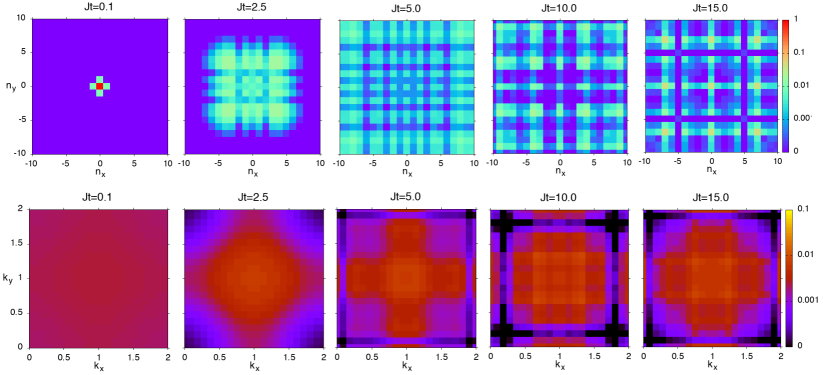
Figure 2: (Color online) Expansion dynamics of the BEC cloud for interaction strength $u=3$, $\rho=1$, and lattice size $21\times 21$. The top row shows the expansion in real space for various times from $tJ=0.1$ to $15$. The color code represents the local condensate occupation numbers in units of the total particle number $N^{0}_{i}(t)/N$. The lattice momentum distribution $n_{\bf k}(t)$ [Eq. (31)] is shown in the bottom row for the corresponding times. Here $k_{x,y}$ are shown in units of $\pi/a$.

III Results

We consider a square optical lattice of size $I\times I$, where $I$ is the odd number of sites along the $x$ or $y$ direction. Each site is addressed by the double index $i\equiv(n_{x},n_{y})$ where $n_{x}$ and $n_{y}$ run from $-(I-1)/2$ to $(I-1)/2$, and summation over $i$ implies summing over all lattice sites. We will impose periodic boundary conditions and define the first Brillouin zone such that the quasimomenta $k_{x},k_{y}\in[0,2\pi/a]$, where $a$ is the lattice constant (see also Figs. 2 and 3). The filling factor is $\rho=N/I^{2}$, where $N$ is the total particle number,

$$N=\sum_{i}N^{0}_{i}(t)+N^{\varphi}_{i}(t)=\sum_{i}\left[|a_{i}(t)|^{2}+{i}\text{F}_{ii}^{G}(t,t)-\frac{1}{2}\right]\,.$$ (28)

In Eq. (28), $N_{i}^{0}(t)$ is the number of condensed particles, while $N^{\varphi}_{i}(t)$ is the particle number in the incoherent cloud, or fluctuation particle number. The total particle number $N$ is conserved. This is obeyed by our conserving approximations (the BHF and the second-order self-consistent approximations)Mauro2015 . We have also confirmed it in our numerics. We study the expansion dynamics in dependence on the interparticle interaction $U$, expressed in dimensionless units as

$$u=\frac{UN}{J}$$ (29)

and express the time in terms of the dimensionless variable $Jt$.

As the initial condition, we assume that at time $t=0$ all particles are condensed in the central site $(0,0)$, that is,

$$a_{i}(0) = \sqrt{\rho I^{2}}\delta_{i0},$$

$$\text{F}_{ij}^{G}(0,0) = -\frac{{i}}{2}\delta_{ij},$$

$$\text{F}_{ij}^{F}(0,0) = 0.$$ (30)

The temporal expansion of the bosonic gas is then expressed in terms of the time-dependent site occupations $N_{i}(t)=N^{0}_{i}(t)+N^{\varphi}_{i}(t)$, the local fluctuation numbers $N^{\varphi}_{i}(t)$, and $n_{\bf k}(t)$, the quasimomentum distribution of the atoms spreading over the optical lattice,

$$n_{\bf k}(t)=\frac{1}{I^{2}}\sum_{ij}e^{{i}{\bf k}({\bf r}_{i}-{\bf r}_{j})}\langle\hat{b}_{i}^{\dagger}(t)\hat{b}_{j}(t)\rangle\,.$$ (31)

III.1 Results without interaction-induced damping

We begin by numerically solving Eqs. (15) which comprise the BHF approximation. This does not take into account inelastic quasiparticle damping effects; however, it captures many of the salient features of the expansion dynamics, namely, occupation-induced shifts of the single-particle energies, effects of the coherent BEC dynamics including selftrapping, and dynamical creation of the incoherent cloud of single-particle excitations beyond the Gross-Pitaevskii equation and its exchange with the BEC.

Figure 2 shows the dynamical evolution of the condensate expansion for $I=21$, $\rho=1$, and $u=3$. The top row displays the site occupations $N_{i}(t)/N$ in real space on a logarithmic scale for different times $Jt$. The expanding cloud reaches the edges of the lattice near $tJ\approx 5$. Thereafter, the local site occupations reappear at the respective, opposite sides of the lattice. For our symmetric time evolution starting in the center of the lattice, this corresponds to reflection from the boundaries in a finite-size lattice. Since the latter situation is more realistic for experiments, we will refer to this reappearance effect as reflection in the following. The interference patterns appearing for times $Jt\geq 5$ indicate the coherence of the condensate part of the cloud. The fluctuation dynamics is not shown, as the local fluctuations amount to less than 1$\%$ of the total population in this case. The fluctuation dynamics will be discussed in detail in Figs. 4 and 5. The bottom row in Fig. 2 presents the lattice-momentum distribution in the first Brillouin zone for the same times. Throughout the time evolution, the momentum distribution is rather broad, showing interference effects of the condensate again for times $Jt\geq 5$. It indicates a rather homogeneous expansion of the cloud, with velocities given by ${\bf v}_{\bf k}=\partial\varepsilon_{\bf k}/\partial{\bf k}$ and the square lattice dispersion $\varepsilon_{\bf k}=-2J[\cos(k_{x}a)+\cos(k_{y}a)]$, as also seen from the real-space pictures.

The expansion dynamics changes drastically when the interaction is increased, as shown in Fig. 3 for $u=7$. The real-space pictures (top row in Fig. 3) show that the BEC cloud expands more slowly, where the cloud separates in a high-density central part and a low-density, halolike structure surrounding it, before the particles get reflected from the boundaries and interference effects set in again. This slow expansion is confirmed by the momentum distribution shown in the bottom row of Fig. 3. Throughout the time evolution, it remains strongly peaked around ${\bf k}=(\pi/a,\pi/a)$ where the group velocity ${\bf v}_{\bf k}$ of the square lattice vanishes. This behavior is similar to the experimental observation Schneider2013 , where for a noninteracting gas a homogenous square spread is observed, whereas for finite interaction a bimodal structure of a slow central cloud surrounded by fast square-shaped background is seen in two dimensions.

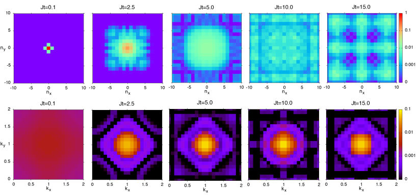
Figure 3: (Color online) Expansion dynamics of the BEC cloud for the same parameters as in Fig. 2, but for interaction strength $u=7$. Distinct self-trapping effects are visible, both in the spatial density distribution (top row) and in the momentum distribution (bottom row).

In order to better understand the behavior of the bimodal structure we plot in Fig. 4 the expansion of the bosonic cloud along the lattice diagonal $n_{x}=n_{y}$ versus time for different values of the interaction $u$ and for both the BEC (top row) and the incoherent cloud (bottom row). While for interaction strength $u\leq 5$ the BEC spreads essentially homogeneously with a slight maximum at the expansion front, the bimodal expansion of the BEC is clearly seen for $u\geq 7$. This can be explained by the self-trapping effect known from bosonic Josephson junctions Smerzi1997 ; Albiez2005 . It is due to an energy mismatch between neighboring sites, that is, it occurs in the nonlinear Gross-Pitaevskii dynamics when the difference between the total condensate energies $u_{i}=UN^{0}_{i}(t)[N^{0}_{i}(t)-1]/2J$ on neighboring sites $i$ and $j$ or neighboring potential wells exceeds a critical value Smerzi1997 ; Mauro2009 . This is fulfilled at the boundaries of the central BEC cloud for $u\geq 7$. As a result, the tunneling of condensate particles from the central, high-density sites to the outer, low-density sites is inhibited, leading to a reduced expansion speed of the central cloud, as seen in the top row of Fig. 4. By contrast, particles on the low-density sites within the halo are not subject to self-trapping and therefore propagate outward ballistically with constant, high speed, in agreement with experiment Schneider2013 . In fact, as seen from Fig. 4, the halo speed in the $x$ direction reaches the Lieb-Robinson limit Lieb1972 , which for our tight-binding square lattice is $v_{x}^{\text{max}}=|{\bf v}_{{\bf k}=(\pi/2a,0)}|=2Ja$. As a result of the different expansion speeds, the central cloud and the halo become spatially separated, leading to a distinct forerunner. This explanation of the bimodal expansion is corroborated by the fact that it is observed only in the expansion of the coherent BEC (top row of Fig. 4), not in the incoherent cloud (bottom row of Fig. 4), as expected from the Gross-Pitaevskii dynamics. Rather, the incoherent excitations are dragged along by the coherent, central cloud and their number is imperceptibly small in the halo for $u\geq 7$. As a remarkable observation, there seems to be an interesting interplay between nonlinear self-trapping and interference for long times. After reflection from the lattice boundaries, the local BEC amplitude may constructively interfere so that locally the selftrapping threshold is reached again, leading to multiple quasilocalized BEC clouds, seen in Fig. 3, top right panel ($Jt=15$), as the nine high-occupation regions. They cannot be a mere interference effect, as they are not observed in Fig. 2 for small interaction ($u=3$).

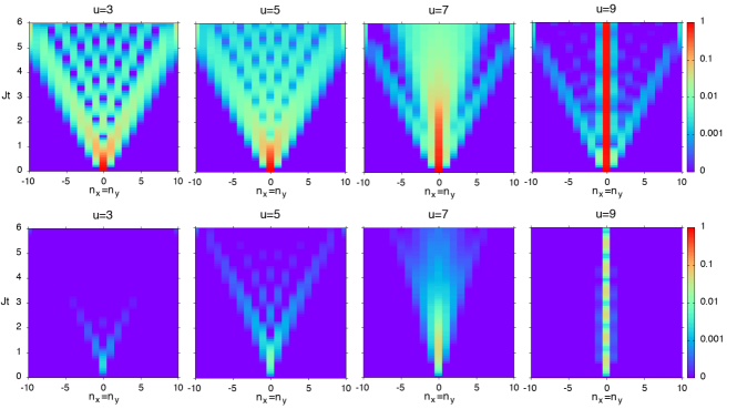
Figure 4: (Color online) Time evolution of the bosonic cloud (top row) and incoherent excitations (bottom row) along the lattice diagonal $n_{x}=n_{y}$ with interaction increasing by steps of two from $3$ to $9$.

The role of the incoherent cloud in the expansion dynamics can be analyzed by monitoring the time evolution of the total fluctuation number and the energy content of the incoherent cloud and the BEC, respectively. Figure 5 shows the noncondensate or fluctuation fraction $N^{\varphi}(t)$ (i.e., the fluctuation number normalized to the total particle number) for various interaction strengths $u$ and filling fractions $\rho$. First, we observe that $N^{\varphi}(t)$ remains in the range of a few percent throughout the time evolution for all parameter values of the ‘$21\times 21$ lattice. For all parameter values, there is a steep, initial rise of the fluctuation fraction within the time of the first tunneling process of the time evolution, $t\approx 1/J$. This is presumably due to the abrupt change of the occupation numbers on the lattice sites neighboring the central one and the consecutive strong perturbation of the BEC. Thereafter, for weak interactions ($u=3,\,5$) the fluctuation fraction increases monotonically with an approximately constant slope. In this weak-interaction regime, $N^{\varphi}(t)$ is approximately inversely proportional to the filling fraction $\rho$, as expected from the perturbative expansion about a homogeneous (position-independent) Gross-Pitaevskii saddle point: The BEC density creates a confining potential for the fluctuations, so increasing density suppresses fluctuations. However, when self-trapping effects set in for strong interaction ($u=7$), the behavior after the initial, strong increase gets reversed. After a pronounced maximum, the total fluctuation density decreases again with time and settles to a reduced, constant value. It seems that the self-trapping-induced, slowed-down dynamics does not support the initial, enhanced fluctuation density, so incoherent excitations recondense into the BEC. In this case, the fluctuation fraction $N^{\varphi}$ also increases with the filling fraction $\rho$.

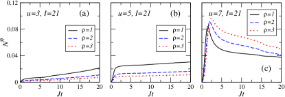
Figure 5: (Color online) Time evolution of the overall quantum fluctuation number $N^{\varphi}$ (normalized to the total particle number $N$) for filling fractions $\rho=1,\,2,\,3$ and (a) $u=3$, (b) $u=5$, and (c) $u=7$.

The time evolution of the kinetic energy $E_{kin}(t)$ and the interaction energy of the total system $E_{int}(t)$ and the respective contributions to the fluctuation energy are shown in Fig. 6. The corresponding energy expectation values are computed from the on-site and nearest-neighbor propagators, respectively, as

$$E_{kin}(t) = E_{kin}^{0}(t)+E_{kin}^{\varphi}(t)$$

$$= -\frac{{i}J}{2}\sum_{\langle i,j\rangle}\,\text{Tr}\left[{\bf C}_{ij}+{\bf F}_{ij}\right]$$

$$E_{int}(t) = E_{int}^{0}(t)+E_{int}^{\varphi}(t)$$

$$= \frac{{i}}{4}\sum_{i}\,\text{Tr}\left[{\bf S}^{HF}_{i}{\bf C}_{ii}+{\bf\Sigma}^{HF}_{i}{\bf F}_{ii}\right],$$

where the superscripts $0$ and $\varphi$ refer to the contributions from condensed atoms and quantum fluctuations, respectively, and $\langle i,j\rangle$ indicates summation over nearest-neighbor sites. While our conserving approximation preserves the total energy conservation, the initially purely interaction energy is quickly transformed into kinetic energy as the central site is depopulated (main panels in Fig. 6). Note that, counterintuitively, this energy transfer is slowed down for strong repulsion, $u=7$, because the depopulation of highly occupied sites is slowed down by selftrapping effects (see also Fig. 4).

The time evolution of the fluctuation energies (insets of Fig. 6) reflects the fluctuation-number dynamics discussed in Fig. 5. For small interaction ($u=3$), after the initial, steep increase, the kinetic fluctuation energy $E_{kin}^{\varphi}(t)$ continues to increase linearly in accordance with the fluctuation number [Fig. 5 (a)], while the interaction energy $E_{int}^{\varphi}(t)$ settles to a constant value. This shows that, although the overall fluctuation number increases with the volume of the cloud, the fluctuation number on each site remains on a constant, small level. On-site two-body interactions among the fluctuations are therefore expected to be small. For strong interaction in the self-trapping regime ($u=7$), the fluctuation kinetic energy follows the evolution of the total fluctuation number as well [Fig. 5 (c)], while the interaction energy settles again to a constant value after a pronounced initial peak.

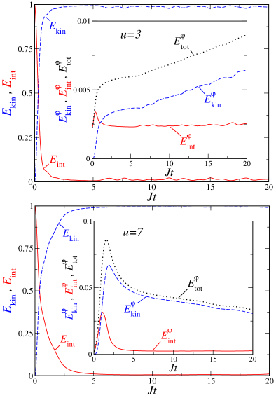
Figure 6: (Color online) Time evolution of the mean kinetic energy (dashed lines) and interaction energy (solid lines) [Eqs. (III.1) and (III.1)], normalized to the total energy $E_{0}=u(N-1)/2$ of the atomic gas loaded on the $21\times 21$ lattice, with $\rho=1$ for interaction parameters $u=3$ (top panel) and $u=7$ (bottom panel). The insets show the kinetic and interaction energies of the quantum fluctuations together with their total energy $E_{tot}^{\varphi}(t)=E_{kin}^{\varphi}(t)+E_{int}^{\varphi}(t)$ (dotted line).

III.2 Small lattices with damping

We now investigate the influence of collisions of the incoherent excitations and damping by solving the second-order self-consistent approximation described by Eqs. (23)–(27). This requires time evolving the propagators and self-energies for two different time arguments. Some details about how to deal with convolution integrals in this case are given in Appendix B. For reasons of numerical costs of computing the second-order self-energies we only consider a $3\times 3$ lattice and limited evolution time here. The corresponding results are shown in Figs. 7 and 8 for all the different inequivalent lattice sites and compared with the BHF results (dashed lines).

First, we note that in the small lattice the fluctuation fraction is generally higher than in the large $21\times 21$ lattice. This may be traced back to the fact that for our initial conditions in the $3\times 3$ lattice the initial condensate number on the central site is smaller than in the $21\times 21$ lattice and thus fluctuations are less strongly suppressed. For the same reason, self-trapping effects are weaker. Second, for $u=3$ the time evolution including collisions of incoherent excitations reproduces the BHF approximation for all considered quantities and filling fractions quantitatively rather well (see Fig. 7), as already conjectured at the end of Sec. III.1. The on-site condensate occupation numbers $N_{i}^{0}(t)$ perform pronounced, weakly damped Josephson-like oscillations Mauro2009 . Finally, for $u=7$ the total local occupation numbers $N_{i}^{0}(t)+N_{i}^{\varphi}(t)$ agree again quantitatively well with the BHF approximation, as seen from Figs. 8(a)–8(c). However, in this case and for $\rho=1$, the fraction of fluctuations produced by strong interaction and second-order collisions, deviates strongly from the prediction of the BHF approximation. This leads to fast condensate depletion on all sites, and condensate oscillations are quickly damped, as seen in Fig. 8(d) and 8(g). On the other hand, as the filling fraction is increased to $\rho=2$ and $3$, the agreement with the BHF approximation is restored for propagation times up to $Jt\approx 4$ [see Fig. 8(e), 8(f), 8(h), and 8(i)]. Note that these filling fractions correspond to initial populations of the central site of 18 and 27, respectively, which are still far below the initial central-site occupation of $21^{2}=441$ for the $21\times 21$ lattice at $\rho=1$. Considering that the importance of fluctuations (and therefore their interactions) decreases with increasing condensate population, we conclude that the BHF results of Sec. III.1 for a $21\times 21$ lattice should be reliable at least for the initial time evolution up to $Jt\approx 5$, even though quasiparticle collisions are not taken into account there. Consequently, the bimodal expansion separated into a strongly populated central cloud and a weak quantum coherent halo should be observable in high-density clouds, similar to the experimental findings of Ref. Schneider2013 . We note that for the discrete density of states of the finite-size lattice, a homogeneous 2D BEC would be thermodynamically stable in equilibrium as long as the particle density does not drop below a critical value $n_{crit}(T)$. Estimating the final-state equilibrium temperature $T_{\infty}$ from the interaction energy per particle of the initial state, we have for our systems $n_{crit}(T_{\infty})={\it O}(10^{-1})$, significantly below the average particle density of 1 per site. Therefore, the condensate depletion is due to the nonequilibrium dynamics rather than a thermodynamical instability.

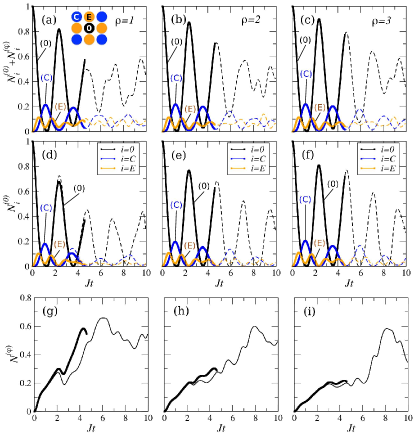
Figure 7: (Color online) Site-resolved expansion in a $3\times 3$ lattice for $u=3$ and different filling factors $\rho=1$, $2$, and $3$. Here $N_{i}^{(0)}(t)$ denotes the condensate number, $N_{i}^{(\varphi)}(t)$ the fluctuation number on site $i$, and $N^{(\varphi)}(t)$ the total number of fluctuations, each normalized to the total particle number $N$. Black, blue (dark gray), and orange (light grey) lines represent the central (0), corner (C), and edge sites (E), respectively, as indicated and visualized by the color-coded lattice shown in the inset. Thick lines represent the solutions of the self-consistent second-order approximation including inelastic collisions; thin or dashed dashed lines correspond to the solutions obtained within the BHF approximation in all panels.

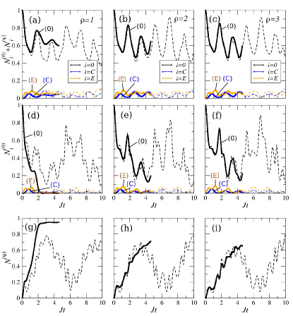
Figure 8: (Color online) Site-resolved expansion in a $3\times 3$ lattice as in Fig. 7, but for interaction strength $u=7$.

IV Conclusion

We have studied the temporal expansion dynamics of an ultracold Bose gas in the two-dimensional Bose-Hubbard model, where initially all bosons are trapped and condensed at the central site of a square lattice. Within our formalism we were able to analyze separately (i) the semiclassical Gross-Pitaevskii dynamics of the BEC, (ii) the dynamics of quantum fluctuations and (iii) their inelastic two-body interactions as well as the mutual influence of these components on each other. After the hopping is switched on, the bosons spread over the lattice in a nontrivial way. We showed that the expansion dynamics depends crucially on interactions. One can clearly distinguish a strongly interacting regime (for our system, $u\geq 7$) when the condensate cloud effectively splits into two parts: a slowly expanding high-density part at the center of the lattice and a fast, quantum coherent, low-density halo or forerunner at the rim of the cloud. This bimodal structure is in qualitative agreement with the experiment Schneider2013 and is interpreted as due to nonlinear selftrapping effects, since doublon dynamics should not play a role in this high-density regime. The existence of a coherent forerunner with average particle number per site of about 1 for strong interactions $u=7,\,9$ (see Fig. 4, top panels) shows that a quantum distillation effect Weiss2015 also exists for high initial particle density. We obtained constant expansion speed, indicative of ballistic motion, for the front of both the BEC and the incoherent cloud (see Fig. 4), as one expects for a coherent wave function. While for the incoherent cloud one might expect diffusive expansion as for classical particles on a lattice, we attribute its linear-in-time expansion to a dragging effect of the incoherent cloud by the BEC. Furthermore, we demonstrated that the velocity of the forerunner is bounded from above and reaches the maximum group velocity of the system, which represents the Lieb-Robinson limit Lieb1972 for this case.

We also showed that in high-density, interacting clouds the quench dynamics leads to an initial, explosive generation of fluctuations, albeit with a small overall amplitude. As the cloud further expands, for weak interaction ($u=3$, $5$) the fluctuation number continues to increase, but linearly in time with a moderate slope. For stronger interaction ($u=7$), the role of the condensate as a confining potential for the fluctuations starts to dominate, so the initially created fluctuation numbers are no longer supported by the further expansion dynamics, leading to a peaklike time evolution of the fluctuation number. In this way, the fluctuations remain confined to a low number in high-density systems for all interaction parameters.

For smaller lattices we studied damping effects due to quasiparticle collisions. Since it is numerically a challenging problem, we reduced the analysis to $3\times 3$ lattices. In this case, the fluctuation numbers are much higher than in larger lattices, as expected. In low-density systems, the collision-induced damping can lead to a fast depletion of the condensate population, transforming the system into an incoherent gas. In the long-time limit, this should lead to a thermal gas Anna2016 above the condensation temperature. For larger filling fractions (or initial central site occupation), however, the coherent BEC dynamics is recovered for significant evolution times. Extrapolating this finding to the large lattice systems, we concluded that the bimodal expansion should be robust against collisions. This analysis shows the possibly important role of fluctuations, depending on the lattice size and interaction also noted in the experiment Schneider2013 . In addition, it provides an explanation why the bimodal expansion was experimentally observed Schneider2013 , despite the ubiquitous presence of fluctuations. In the future it will be interesting to study collision effects for disordered as well as periodically driven Bose-Hubbard lattices.

Appendix A Symmetry relations

Our equations simplify if we make use of the symmetry relations listed below. For the components of the spectral function and statistical functions the following equations hold:

$$\text{A}_{ij}^{\overline{G}}(t,t^{\prime}) =-\text{A}_{ij}^{G}(t,t^{\prime})^{*}=-\text{A}_{ji}^{G}(t^{\prime},t)$$ (34)

$$\text{A}_{ij}^{\overline{F}}(t,t^{\prime}) =-\text{A}_{ij}^{F}(t,t^{\prime})^{*}=\text{A}_{ji}^{F}(t^{\prime},t)^{*}$$

$$\text{F}_{ij}^{\overline{G}}(t,t^{\prime}) =-\text{F}_{ij}^{G}(t,t^{\prime})^{*}=\text{F}_{ji}^{G}(t^{\prime},t)$$

$$\text{F}_{ij}^{\overline{F}}(t,t^{\prime}) =-\text{F}_{ij}^{F}(t,t^{\prime})^{*}=-\text{F}_{ji}^{F}(t^{\prime},t)^{*}.$$

The selfenergies which enter Eqs. (10)–(12) also obey the symmetry relations

$$\gamma_{ij}^{G}(t,t^{\prime})^{*} =-\gamma_{ij}^{\overline{G}}(t,t^{\prime})=\gamma_{ji}^{G}(t^{\prime},t)$$ (35)

$$\gamma_{ij}^{F}(t,t^{\prime})^{*} =-\gamma_{ij}^{\overline{F}}(t,t^{\prime})=\gamma_{ji}^{\overline{F}}(t^{\prime},t)$$

$$\Gamma_{ij}^{G}(t,t^{\prime})^{*} =-\Gamma_{ij}^{\overline{G}}(t,t^{\prime})=\Gamma_{ji}^{G}(t^{\prime},t)$$

$$\Gamma_{ij}^{F}(t,t^{\prime})^{*} =-\Gamma_{ij}^{\overline{F}}(t,t^{\prime})=\Gamma_{ji}^{\overline{F}}(t^{\prime},t)$$

$$\Pi_{ij}^{G}(t,t^{\prime})^{*} =-\Pi_{ij}^{\overline{G}}(t,t^{\prime})=-\Pi_{ji}^{G}(t^{\prime},t)$$

$$\Pi_{ij}^{F}(t,t^{\prime})^{*} =-\Pi_{ij}^{\overline{F}}(t,t^{\prime})=-\Pi_{ji}^{\overline{F}}(t^{\prime},t)\,.$$

Appendix B Convolution integrals in equations of motion

We can use the symmetry relations listed in Appendix A also in the convolution integrals which enter our equations of motion (23)–(II.3). Consider, for example, the integrals in Eq. (II.3),

$$-{i}\sum_{k}\int\limits_{0}^{t}d\overline{t}[\Gamma^{G}_{ik}(t,\overline{t})\text{F}^{G}_{kj}(\overline{t},t^{\prime})+\Gamma^{F}_{ik}(t,\overline{t})\text{F}^{\overline{F}}_{kj}(\overline{t},t^{\prime})]+{i}\sum_{k}\int\limits_{0}^{t^{\prime}}d\overline{t}[\Pi^{G}_{ik}(t,\overline{t})\text{A}^{G}_{kj}(\overline{t},t^{\prime})+\Pi^{F}_{ik}(t,\overline{t})\text{A}^{\overline{F}}_{kj}(\overline{t},t^{\prime})].$$ (36)

The symmetry relations allow us to split the interval of integration in such a way that we can rewrite the integrals with the arguments corresponding to the later time as first arguments. Hence, we get, for the integral (36),

$$\phantom{+}{i}\sum_{k}\int\limits_{0}^{t^{\prime}}d\overline{t}[\Gamma^{G}_{ik}(t,\overline{t})\text{F}^{G}_{jk}(t^{\prime},\overline{t})^{*}+\Gamma^{F}_{ik}(t,\overline{t})\text{F}^{F}_{jk}(t^{\prime},\overline{t})^{*}] -{i}\sum_{k}\int\limits_{t^{\prime}}^{t}d\overline{t}[\Gamma^{G}_{ik}(t,\overline{t})\text{F}^{G}_{kj}(\overline{t},t^{\prime})-\Gamma^{F}_{ik}(t,\overline{t})\text{F}^{F}_{kj}(\overline{t},t^{\prime})^{*}]$$ (37)

$$+{i}\sum_{k}\int\limits_{0}^{t^{\prime}}d\overline{t}[\Pi^{G}_{ik}(t,\overline{t})\text{A}^{G}_{jk}(t^{\prime},\overline{t})^{*}+\Pi^{F}_{ik}(t,\overline{t})\text{A}^{F}_{jk}(t^{\prime},\overline{t})].$$

We proceed in an analogous way for the other integrals of Eqs. (23)–(II.3) and then solve the final system of equations numerically.

References

- (1)
- (2) M. P. A. Fisher, P. B. Weichman, G. Grinstein, D. S. Fisher, Boson localization and the superfluid-insulator transition, Phys. Rev. B 40, 546 (1989).
- (3) M. Greiner, O. Mandel, T. Esslinger, T. W. Hänsch, and I. Bloch, Quantum phase transition from a superfluid to a Mott insulator in a gas of ultracold atoms, Nature (London) 419, 39 (2002).
- (4) A. Polkovnikov, K. Sengupta, A. Silva, and M. Vengalattore, Colloquium: Nonequilibrium dynamics of closed interacting quantum systems, Rev. Mod. Phys. 83, 863 (2011).
- (5) T. Langen, R. Geiger, J. Schmiedmayer, Ultracold atoms out of equilibrium, Annu. Rev. Condens. Matter Phys. 6, 201 (2015).
- (6) J. Eisert, M. Friesdorf, and C. Gogolin, Quantum many-body systems out of equilibrium, Nature Phys. 11, 124 (2015).
- (7) G. Gogolin and J. Eisert, Equilibration, thermalisation, and the emergence of statistical mechanics in closed quantum systems, Rep. Prog. Phys. 79, 056001 (2016).
- (8) L. d’Alessio, Y. Kafri, A. Polkovnikov, and M. Rigol From quantum chaos and eigenstate thermalization to statistical mechanics and thermodynamics, Adv. Phys. 65, 239 (2016).
- (9) J. P. Ronzheimer, M. Schreiber, S. Braun, S. S. Hodgman, eS. Langer, I. P. McCulloch, F. Heidrich-Meisner, I. Bloch, and U. Schneider, Expansion Dynamics of Interacting Bosons in Homogeneous Lattices in One and Two Dimensions, Phys. Rev. Lett. 110, 205301 (2013).
- (10) A. Reinhard, J.-F. Riou, L. A. Zundel, D. S. Weiss, S. Li, A. M. Rey, and R. Hipolito, Self-Trapping in an Array of Coupled 1D Bose Gases, Phys. Rev. Lett. 110, 033001 (2013).
- (11) L. Xia, L. A. Zundel, J. Carrasquilla, A. Reinhard, J. M. Wilson, M. Rigol, D. S. Weiss, Quantum distillation and confinement of vacancies in a doublon sea, Nature Phys. 11, 316 (2015).
- (12) L. Vidmar, J. P. Ronzheimer, M. Schreiber, S. Braun, S. S. Hodgman, S. Langer, F. Heidrich-Meisner, I. Bloch, and U. Schneider Dynamical Quasicondensation of Hard-Core Bosons at Finite Momenta Phys. Rev. Lett. 115, 175301 (2015).
- (13) M. Jreissaty, J. Carrasquilla, F. A. Wolf, and M. Rigol, Expansion of Bose-Hubbard Mott insulators in optical lattices, Phys. Rev. A 84, 043610 (2011).
- (14) A. Jreissaty, J. Carrasquilla, and M. Rigol, Self-trapping in the two-dimensional Bose-Hubbard model Phys. Rev. A 88, 031606(R) (2013).
- (15) S. Li, S. R. Manmana, A. M. Rey, R. Hipolito, A. Reinhard, J.-F. Riou, L. A. Zundel, and D. S. Weiss, Self-trapping dynamics in a two-dimensional optical lattice, Phys. Rev. A 88, 023419 (2013).
- (16) L. Vidmar, S. Langer, I. P. McCulloch, U. Schneider, U. Schollwöck, and F. Heidrich-Meisner, Sudden expansion of Mott insulators in one dimension, Phys. Rev. B 88, 235117 (2013).
- (17) C. degli Esposti Boschi, E. Ercolessi, L. Ferrari, P. Naldesi, F. Ortolani, and L. Taddia, Bound states and expansion dynamics of interacting bosons on a one-dimensional lattice, Phys. Rev. A 90, 043606 (2014).
- (18) J. Hauschild, F. Pollmann, and F. Heidrich-Meisner, Sudden expansion and domain-wall melting of strongly interacting bosons in two-dimensional optical lattices and on multileg ladders, Phys. Rev. A 92, 053629 (2015).
- (19) Wei Xu and Marcos Rigol, Expansion of one-dimensional lattice hard-core bosons at finite temperature, Phys. Rev. A 95, 033617 (2017).
- (20) B. Shapiro, Expansion of a Bose-Einstein Condensate in the Presence of Disorder, Phys.Rev. Lett. 99, 060602 (2007).
- (21) S. Aktas and U. Atav, Expansion Dynamics of Two Dimensional Extended Bose-Hubbard Model, arXiv:1408.3323 (2014).
- (22) D. Muth, D. Petrosyan, and M. Fleischhauer, Dynamics and evaporation of defects in Mott-insulating clusters of boson pairs, Phys. Rev. A 85, 013615 (2012).
- (23) M. Trujillo-Martinez, A. Posazhennikova, and J. Kroha, Nonequilibrium Josephson Oscillations in Bose-Einstein Condensates without Dissipation, Phys. Rev. Lett. 103, 105302 (2009).
- (24) M. Trujillo-Martinez, A. Posazhennikova, and J. Kroha, Temporal non-equilibrium dynamics of a Bose-Josephson junction in presence of incoherent excitations, New J. Phys. 17, 013006 (2015).
- (25) A. Posazhennikova, M. Trujillo-Martinez, and J. Kroha, Inflationary Quasiparticle Creation and Thermalization Dynamics in Coupled Bose-Einstein Condensates, Phys. Rev. Lett. 116, 225304 (2016).
- (26) A. Posazhennikova, M. Trujillo-Martinez, and J. Kroha, Thermalization of isolated Bose-Einstein condensates by dynamical heat bath Generation, Ann. Phys. (Berlin) 530, 1700124 (2018).
- (27) T. Lappe, A. Posazhennikova, and J. Kroha, Fluctuation damping of isolated, oscillating Bose-Einstein condensates, Phys. Rev. A 98, 023626 (2018).
- (28) P. Barmettler, D. Poletti, M. Cheneau, and C. Kollath, Propagation front of correlations in an interacting Bose gas Phys. Rev. A 85, 053625 (2012).
- (29) L. P. Kadanoff, and G. Baym, Quantum Statistical Mechanics, (Benjamin, Menlo Park, 1962).
- (30) L. M. Sieberer, M. Buchhold, and S. Diehl, Keldysh field theory for driven open quantum systems, Rep. Prog. Phys. 79, 096001 (2016).
- (31) A. Smerzi, S. Fantoni, S. Giovanazzi, and S. R. Shenoy, Quantum coherent atomic tunneling between two trapped Bose-Einstein condensates, Phys. Rev. Lett. 79, 4950 (1997).
- (32) M. Albiez, R. Gati, J. Fölling, S. Hunsmann, M. Cristiani, and M. K. Oberthaler, Direct Observation of Tunneling and Nonlinear Self-Trapping in a Single Bosonic Josephson Junction, Phys. Rev. Lett. 95, 010402 (2005).
- (33) E. Lieb and D. Robinson, The finite group velocity of quantum spin systems, Commun. Math. Phys. 28, 251, (1972).
- (34) D. Jaksch, C. Bruder, J. I. Cirac, C. W. Gardiner, and P. Zoller, Cold Bosonic Atoms in Optical Lattices, Phys. Rev. Lett. 81, 3108 (1998).
- (35) A. Griffin, T. Nikuni, and E. Zaremba, Bose-Condensed Gases at Finite Temperatures (Cambridge University Press, Cambridge, 2009).
- (36) J. Rammer, Quantum Field Theory of Non-Equilibrium States (Cambridge University Press, 2007).