A stochastic control problem with linearly bounded control rates in a Brownian model

Abstract.

Aiming for more realistic optimal dividend policies, we consider a stochastic control problem with linearly bounded control rates using a performance function given by the expected present value of dividend payments made up to ruin. In a Brownian model, we prove the optimality of a member of a new family of control strategies called delayed linear control strategies, for which the controlled process is a refracted diffusion process. For some parameters specifications, we retrieve the strategy initially proposed in [avanzi-wong_2012] to regularize dividend payments, which is more consistent with actual practice.

1. Introduction and main result

In this paper, we consider an optimal stochastic control problem with absolutely continuous and linearly bounded control strategies in a Brownian model. Our problem is a version of de Finetti’s dividend problem in which payment/control strategies can be at most a (fixed) fraction of the current wealth/state. For this problem, an optimal strategy is formed by a delayed linear control strategy. Loosely speaking, for such a strategy, no dividends are paid below a barrier and level-dependent dividend payments are made when the process is above that barrier, allowing for more regular dividend payments over time. As the underlying state process is a Brownian motion, in order to solve this stochastic control problem, we study a specific refracted diffusion process, i.e., a dynamic alternating between a Brownian motion with drift and an Ornstein-Uhlenbeck process.

1.1. Model and problem formulation

On a filtered probability space $\left(\Omega,\mathcal{F},\left\{\mathcal{F}_{t},t\geq 0\right\},\mathbb{P}\right)$, let $X=\left\{X_{t},t\geq 0\right\}$ be a Brownian motion with drift, i.e.

$$\mathrm{d}X_{t}=\mu\mathrm{d}t+\sigma\mathrm{d}B_{t},$$ (1)

where $\mu\in\mathbb{R}$ and $\sigma>0$, and where $B=\left\{B_{t},t\geq 0\right\}$ is a standard Brownian motion. Using the language of ruin theory, $X$ is the (uncontrolled) surplus process.

A dividend strategy $\pi$ is represented by a non-decreasing, left-continuous and adapted stochastic process $L^{\pi}=\left\{L^{\pi}_{t},t\geq 0\right\}$, where $L^{\pi}_{t}$ represents the cumulative amount of dividends paid up to time $t$ under this strategy. For a given strategy $\pi$, the corresponding controlled surplus process $U^{\pi}=\left\{U^{\pi}_{t},t\geq 0\right\}$ is defined by $U^{\pi}_{t}=X_{t}-L^{\pi}_{t}$.

While de Finetti’s classical dividend problem is a singular stochastic control problem, we are interested in an adaptation where the admissible strategies are absolutely continuous with a linearly bounded rate.

Definition 1.1 (Admissible strategies).

Fix a constant $K>0$. A strategy $\pi$ is said to be admissible if it is absolutely continuous and linearly bounded, i.e., $\mathrm{d}L_{t}^{\pi}=\ell^{\pi}_{t}\mathrm{d}t$, with $0\leq\ell^{\pi}_{t}\leq KU^{\pi}_{t}$, for all $t>0$. The set of admissible dividend strategies will be denoted by $\Pi^{K}$.

Thus, for an admissible strategy $\pi$, we have

$$\mathrm{d}U^{\pi}_{t}=\mathrm{d}X_{t}-\ell^{\pi}_{t}\mathrm{d}t=\left(\mu-\ell^{\pi}_{t}\right)\mathrm{d}t+\sigma\mathrm{d}B_{t}.$$

For a given discounting rate $q\geq 0$, the value/performance function associated to an admissible strategy $\pi$ and initial value $U_{0}=X_{0}=x$ is given by

$$v_{\pi}(x)=\mathbb{E}_{x}\left[\int_{0}^{\sigma^{\pi}}\mathrm{e}^{-qt}\ell^{\pi}_{t}\mathrm{d}t\right]$$

where $\sigma^{\pi}=\inf\left\{t>0\colon U_{t}^{\pi}<0\right\}$. Note that $v_{\pi}(x)=0$ for all $x\leq 0$. For notational simplicity, but without loss of generality, we have chosen the ruin level to be $0$, as it is often the case in ruin theory when dealing with space-homogeneous surplus processes.

The goal of this stochastic control problem is to find the optimal value function $v_{\ast}$ defined by

$$v_{\ast}(x)=\sup_{\pi\in\Pi^{K}}v_{\pi}(x)$$

and, if it exists, an optimal strategy $\pi_{\ast}\in\Pi^{K}$ such that

$$v_{\pi_{\ast}}(x)=v_{\ast}(x),$$

for all $x>0$.

1.2. Main result

As alluded to above, the optimal control strategy is of bang-bang type, i.e., dividends are either paid out at the maximal surplus-dependent rate or nothing is paid, depending on the value of the controlled process. Mathematically, let us define the following refracted diffusion process: for fixed $b,K\geq 0$, let $U^{b}=\left\{U^{b}_{t},t\geq 0\right\}$ be given by

$$\mathrm{d}U^{b}_{t}=\left(\mu-KU^{b}_{t}\mathbf{1}_{\{U^{b}_{t}>b\}}\right)\mathrm{d}t+\sigma\mathrm{d}B_{t}.$$ (2)

We prove the existence of a strong solution to this stochastic differential equation in Appendix A. This process is the controlled process associated to the (admissible) control strategy $\ell^{b}_{t}=KU^{b}_{t}\mathbf{1}_{\{U^{b}_{t}>b\}}$, which consists of paying out at the maximal surplus-dependent rate $K$ when the controlled process is above level $b$ and pay nothing below $b$. This control strategy will be denoted by $\pi_{b}$ and called a delayed linear control strategy at level $b$ with rate $K$, when $b>0$, and simply a linear control strategy with rate $K$, when $b=0$. In both cases, it is an admissible strategy, i.e., $\pi_{b}\in\Pi^{K}$ for any $b\geq 0$.

Define

$$\Delta=-H^{(q)}_{K}(0)/H^{(q)\prime}_{K}(0),$$ (3)

where the function $H^{(q)}_{K}$ is defined in (9). Note that $\Delta$ depends on both the control problem parameters $q$ and $K$ and the model parameters $\mu$ and $\sigma$. Define also $b^{\ast}$ as the (unique) root of Equation (10); see below.

Here is an explicit solution to the control problem:

Theorem 1.2.

Fix $q>0$ and $K>0$. The following hold:

• If $\mu K/q^{2}\leq\Delta$, then the linear control strategy with rate $K$ is optimal.

• If $\mu K/q^{2}>\Delta$, then the delayed linear control strategy at level $b^{\ast}>0$ with rate $K$ is optimal.

1.3. Related literature

If a delayed linear control strategy at level $b>0$ with rate $K$ is implemented, then dividends are paid continuously only when the process is above level $b$, according to an Ornstein-Uhlenbeck process with mean-reverting level $\mu/K$. In other words, when $b>0$, we have to wait for sufficient capital before paying out dividends according to this linear strategy. If the linear strategy with rate $K$ is implemented, i.e., when $b=0$, then dividends are paid without interruption up to the time of ruin, according to an Ornstein-Uhlenbeck process with mean-reverting level $\mu/K$. This last strategy is the one initally proposed in [avanzi-wong_2012] to regularize dividend payments; it is also studied in [albrecher-cani_2017] for a compound Poisson process with drift. In Section 6 of [avanzi-wong_2012], the authors hinted at delayed linear control strategies. In some sense, delaying dividend payments brings additional safety by avoiding payments when the process is close to the ruin level. Theorem 1.2 tells us that, for our control problem, either the optimal strategy is a linear control strategy, as studied in [avanzi-wong_2012], or it is a member of the family of delayed linear control strategies. In the latter case, Proposition 2.2 tells us how to find the optimal level $b^{\ast}$.

Note that our problem has similarities with another variation on de Finetti’s optimal dividends problem, in which admissible strategies have a bounded rate, i.e., $0\leq\ell^{\pi}_{t}\leq\widetilde{K}$, for all $t>0$, for a fixed constant $\widetilde{K}$; see, e.g., [jeanblanc-shiryaev_1995]. However, for that problem, the optimal control process is a two-valued Brownian motion with drift, also called a refracted Brownian motion with drift. In the classical de Finetti’s control problem, admissible strategies are not necessarily absolutely continuous nor bounded. For the classical problem, the optimal control process is a reflected Brownian motion with drift and the optimal reflection level is known to be

$$c^{\ast}=\frac{\sigma^{2}}{\sqrt{\mu^{2}+2q\sigma^{2}}}\ln\left(\frac{\mu+\sqrt{\mu^{2}+2q\sigma^{2}}}{-\mu+\sqrt{\mu^{2}+2q\sigma^{2}}}\right).$$ (4)

Intuitively, in our problem, if $K$ becomes large, then we should get closer to the classical problem.

The rest of the paper is organized as follows. In Section 2, we provide background material on Ornstein-Uhlenbeck diffusion processes, we compute the value function of an arbitrary (delayed) linear control strategy and then we find the (candidate) optimal barrier level $b^{\ast}$. In Section 3, we give a verification lemma for this control problem and prove Theorem 1.2. Finally, Section 4 aims at giving a second look at the main results with a short discussion and numerical illustrations. More technical material is provided in the appendices, including a proof for the existence of a refracted Ornstein-Uhlenbeck diffusion process and ordinary differential equations related to the control problem.

2. Delayed linear control strategies

Before computing the value function of an arbitrary linear control strategy and then finding the optimal barrier level, let us recall some results about Ornstein-Uhlenbeck diffusion processes.

2.1. Preliminaries on Ornstein-Uhlenbeck diffusion processes

First, let us recall some results on first-passage problems for the Brownian motion with drift $X$, given in (1), and the Ornstein-Uhlenbeck diffusion process $U=\left\{U_{t},t\geq 0\right\}$ given by

$$\mathrm{d}U_{t}=\left(\mu-KU_{t}\right)\mathrm{d}t+\sigma\mathrm{d}B_{t},$$ (5)

where $K\geq 0$. Clearly, if $K=0$, then $U=X$. In what follows, we will use the following notation: the law of $U$ when starting from $U_{0}=x$ is denoted by $\mathbb{P}^{(K)}_{x}$ and the corresponding expected value operator by $\mathbb{E}^{(K)}_{x}$. Define the following first-passage stopping times: for $a\in\mathbb{R}$, let $\tau_{a}=\inf\left\{t\colon U_{t}=a\right\}$.

In what follows, we assume $q>0$. First, we consider the case $K=0$, i.e. the case when $U=X$ is a Brownian motion with drift. It is known (see, e.g., [kyprianou_2014]) that, for $0\leq x\leq a$,

$$\mathbb{E}^{(0)}_{x}\left[\mathrm{e}^{-q\tau_{a}}\mathbf{1}_{\{\tau_{a}<\tau_{0}\}}\right]=\frac{W^{(q)}(x)}{W^{(q)}(a)},$$ (6)

where, for $x>0$,

$$W^{(q)}(x)=\frac{2}{\sqrt{\mu^{2}+2q\sigma^{2}}}\mathrm{e}^{-(\mu/\sigma^{2})x}\sinh\left((1/\sigma^{2})\sqrt{\mu^{2}+2q\sigma^{2}}x\right)$$ (7)

and, for $x\leq 0$, $W^{(q)}(x)=0$. It is known that $W^{(q)\prime}$ is convex.

Now, we consider the case $K>0$, i.e., the case when $U$ is an Ornstein-Uhlenbeck diffusion process. It is known (see, e.g., [alili-et-al_2005] and references therein) that $U$ is a recurrent diffusion, so $\tau_{a}$ is finite, almost surely. If $\mu=0$ and $\sigma=1$, then, for $x<a$,

$$\mathbb{E}^{(K)}_{x}\left[\mathrm{e}^{-q\tau_{a}}\mathbf{1}_{\{\tau_{a}<\infty\}}\right]=\frac{\mathrm{e}^{Kx^{2}/2}\mathrm{D}_{-q/K}\left(-x\sqrt{2K}\right)}{\mathrm{e}^{Ka^{2}/2}\mathrm{D}_{-q/K}\left(-a\sqrt{2K}\right)},$$

where $\mathrm{D}_{-\lambda}$ is the parabolic cylinder function defined, for $x\in\mathbb{R}$, by

$$\mathrm{D}_{-\lambda}(x)=\frac{1}{\Gamma(\lambda)}\mathrm{e}^{-x^{2}/4}\int_{0}^{\infty}t^{\lambda-1}\mathrm{e}^{-xt-t^{2}/2}\mathrm{d}t.$$

We see that $x\mapsto\mathrm{e}^{Kx^{2}/2}\mathrm{D}_{-q/K}\left(-x\sqrt{2K}\right)$ is increasing and convex.

Consequently, for $\mu\in\mathbb{R}$ and $\sigma>0$, we can deduce that, for $x\geq a$,

$$\mathbb{E}^{(K)}_{x}\left[\mathrm{e}^{-q\tau_{a}}\mathbf{1}_{\{\tau_{a}<\infty\}}\right]=\frac{H^{(q)}_{K}\left(x\right)}{H^{(q)}_{K}\left(a\right)},$$ (8)

where

$$H^{(q)}_{K}(x):=\mathrm{e}^{K\left(x-\mu/K\right)^{2}/2\sigma^{2}}\mathrm{D}_{-q/K}\left(\left(\frac{x-\mu/K}{\sigma}\right)\sqrt{2K}\right).$$ (9)

It is easy to verify that $H^{(q)}_{K}$ is convex.

For more analytical properties of $W^{(q)}$ and $H^{(q)}_{K}$, see Appendix B.

2.2. Value function and optimal barrier level

Fix $q>0$ and $K>0$. Recall that, for an arbitrary $b\geq 0$, the process $U^{b}=\left\{U^{b}_{t},t\geq 0\right\}$ is the controlled process associated to the delayed linear strategy $\pi_{b}\in\Pi^{K}$. This refracted diffusion process is the solution to the SDE in (2), which we recall here:

$$\mathrm{d}U^{b}_{t}=\left(\mu-KU^{b}_{t}\mathbf{1}_{\{U^{b}_{t}>b\}}\right)\mathrm{d}t+\sigma\mathrm{d}B_{t}.$$

Denote the ruin time of this process by $\sigma^{b}=\inf\left\{t>0\colon U_{t}^{b}<0\right\}$. Note that, if $b=0$, then $U^{0}=\left\{U^{0}_{t},0\leq t\leq\sigma^{0}\right\}$ has the same law as $U=\left\{U_{t},0\leq t\leq\tau_{0}\right\}$, where $U$ is the Ornstein-Uhlenbeck process defined in (5).

Denote the value function associated to $\pi_{b}$ by

$$v_{b}(x)=\mathbb{E}_{x}\left[\int_{0}^{\sigma^{b}}\mathrm{e}^{-qt}\left(KU^{b}_{t}\mathbf{1}_{\{U^{b}_{t}>b\}}\right)\mathrm{d}t\right],\quad x\geq 0.$$

Proposition 2.1.

For $b\geq 0$, we have

$$v_{b}(x)=\begin{cases}\frac{K}{q+K}C_{b}W^{(q)}(x)&\text{if $0\leq x\leq b$,}\\ \frac{K}{q+K}\left[x+\frac{\mu}{q}+D_{b}H^{(q)}_{K}(x)\right]&\text{if $x>b$,}\end{cases}$$

where

$$C_{b}=\frac{H^{(q)}_{K}(b)-\left(b+\frac{\mu}{q}\right)H^{(q)\prime}_{K}(b)}{W^{(q)\prime}(b)H^{(q)}_{K}(b)-W^{(q)}(b)H^{(q)\prime}_{K}(b)}\qquad\text{and}\qquad D_{b}=\frac{W^{(q)}(b)-\left(b+\frac{\mu}{q}\right)W^{(q)\prime}(b)}{W^{(q)\prime}(b)H^{(q)}_{K}(b)-W^{(q)}(b)H^{(q)\prime}_{K}(b)}.$$

Proof.

Fix $b>0$. First assume that $0<x\leq b$. By the strong Markov property, we have

$$v_{b}(x)=\mathbb{E}^{(0)}_{x}\left[\mathrm{e}^{-q\tau_{b}}\mathbf{1}_{\{\tau_{b}<\tau_{0}\}}\right]v_{b}(b)=\frac{W^{(q)}(x)}{W^{(q)}(b)}v_{b}(b),$$

where we used the identity in (6). Now, if we assume that $x>b$, then by the strong Markov property we have

$$v_{b}(x)=K\mathbb{E}^{(K)}_{x}\left[\int_{0}^{\tau_{b}}\mathrm{e}^{-qt}U_{t}\mathrm{d}t\right]+\mathbb{E}^{(K)}_{x}\left[\mathrm{e}^{-q\tau_{b}}\mathbf{1}_{\{\tau_{b}<\infty\}}\right]v_{b}(b),$$

where, using the identity in (8) and using the strong Markov property one last time (as in [avanzi-wong_2012]),

$$\mathbb{E}^{(K)}_{x}\left[\int_{0}^{\tau_{b}}\mathrm{e}^{-qt}U_{t}\mathrm{d}t\right]=\mathbb{E}^{(K)}_{x}\left[\int_{0}^{\infty}\mathrm{e}^{-qt}U_{t}\mathrm{d}t\right]-\mathbb{E}^{(K)}_{x}\left[\mathrm{e}^{-q\tau_{b}}\mathbf{1}_{\{\tau_{b}<\infty\}}\right]\mathbb{E}^{(K)}_{b}\left[\int_{0}^{\infty}\mathrm{e}^{-qt}U_{t}\mathrm{d}t\right].$$

It is well known that, for $t\geq 0$,

$$\mathbb{E}^{(K)}_{x}\left[U_{t}\right]=x\mathrm{e}^{-Kt}+\frac{\mu}{K}\left(1-\mathrm{e}^{-Kt}\right),$$

so we have

$$\mathbb{E}^{(K)}_{x}\left[\int_{0}^{\infty}\mathrm{e}^{-qt}U_{t}\mathrm{d}t\right]=\frac{1}{q+K}\left(x+\frac{\mu}{q}\right).$$

Consequently

$$v_{b}(x)=\begin{cases}\frac{W^{(q)}(x)}{W^{(q)}(b)}v_{b}(b)&\text{if $0\leq x\leq b$,}\\ \frac{K}{q+K}\left(x+\frac{\mu}{q}\right)+\left[v_{b}(b)-\frac{K}{q+K}\left(b+\frac{\mu}{q}\right)\right]\frac{H^{(q)}_{K}(x)}{H^{(q)}_{K}(b)}&\text{if $x>b$.}\end{cases}$$

To compute $v_{b}(b)$, we will use approximations of the delayed linear strategy at level $b$. Fix $n\geq 1$ and let us implement the following strategy: when the (controlled) process reaches $b$, then dividends are paid continuously at rate $K$ until the controlled process goes back to $b-1/n$; dividend payments resume when the controlled process reaches $b$ again. Denote this strategy by $\overline{\pi}_{b}^{n}$ and its value function by $\overline{v}_{b}^{n}$. Clearly, $v_{b}(b)\leq\overline{v}_{b}^{n}(b)$ and thus $v_{b}(b)\leq\lim_{n\to\infty}\overline{v}_{b}^{n}(b)$.

As for $v_{b}$ above, we have the following decompositions:

$$\overline{v}_{b}^{n}(b-1/n)=\mathbb{E}^{(0)}_{b-1/n}\left[\mathrm{e}^{-q\tau_{b}}\mathbf{1}_{\{\tau_{b}<\tau_{0}\}}\right]\overline{v}_{b}^{n}(b),$$

and

$$\overline{v}_{b}^{n}(b)=\mathbb{E}^{(K)}_{b}\left[\int_{0}^{\tau_{b-1/n}}\mathrm{e}^{-qt}KU_{t}\mathrm{d}t\right]+\mathbb{E}^{(K)}_{b}\left[\mathrm{e}^{-q\tau_{b-1/n}}\mathbf{1}_{\{\tau_{b-1/n}<\infty\}}\right]\overline{v}_{b}^{n}(b-1/n).$$

Solving for $\overline{v}_{b}^{n}(b)$, we get

$$\overline{v}_{b}^{n}(b)=\frac{\mathbb{E}^{(K)}_{b}\left[\int_{0}^{\tau_{b-1/n}}\mathrm{e}^{-qt}KU_{t}\mathrm{d}t\right]}{1-\mathbb{E}^{(0)}_{b-1/n}\left[\mathrm{e}^{-q\tau_{b}}\mathbf{1}_{\{\tau_{b}<\tau_{0}\}}\right]\mathbb{E}^{(K)}_{b}\left[\mathrm{e}^{-q\tau_{b-1/n}}\mathbf{1}_{\{\tau_{b-1/n}<\infty\}}\right]}.$$

Since

$$\mathbb{E}^{(K)}_{b}\left[\int_{0}^{\tau_{b-1/n}}\mathrm{e}^{-qt}KU_{t}\mathrm{d}t\right] =\frac{K}{q+K}\left(b+\frac{\mu}{q}\right)-\frac{K}{q+K}\left((b-1/n)+\frac{\mu}{q}\right)\frac{H^{(q)}_{K}(b)}{H^{(q)}_{K}\left(b-1/n\right)},$$

$$\mathbb{E}^{(0)}_{b-1/n}\left[\mathrm{e}^{-q\tau_{b}}\mathbf{1}_{\{\tau_{b}<\tau_{0}\}}\right] =\frac{W^{(q)}(b-1/n)}{W^{(q)}(b)},$$

$$\mathbb{E}^{(K)}_{b}\left[\mathrm{e}^{-q\tau_{b-1/n}}\mathbf{1}_{\{\tau_{b-1/n}<\infty\}}\right] =\frac{H^{(q)}_{K}(b)}{H^{(q)}_{K}\left(b-1/n\right)},$$

dividing by $1/n$ and taking the limit when $n\to\infty$, we get

$$n\mathbb{E}^{(K)}_{b}\left[\int_{0}^{\tau_{b-1/n}}\mathrm{e}^{-qt}KU_{t}\mathrm{d}t\right]\longrightarrow_{n\to\infty}\frac{K}{q+K}-\frac{K}{q+K}\left(b+\frac{\mu}{q}\right)\frac{H^{(q)\prime}_{K}(b)}{H^{(q)}_{K}(b)}$$

and

$$n\left\{1-\mathbb{E}^{(0)}_{b-1/n}\left[\mathrm{e}^{-q\tau_{b}}\mathbf{1}_{\{\tau_{b}<\tau_{0}\}}\right]\mathbb{E}^{(K)}_{b}\left[\mathrm{e}^{-q\tau_{b-1/n}}\mathbf{1}_{\{\tau_{b-1/n}<\infty\}}\right]\right\}\longrightarrow_{n\to\infty}\frac{W^{(q)\prime}(b)}{W^{(q)}(b)}-\frac{H^{(q)\prime}_{K}(b)}{H^{(q)}_{K}(b)}.$$

Putting the pieces together, we finally get

$$\lim_{n\to\infty}\overline{v}_{b}^{n}(b)=\frac{\frac{K}{q+K}-\frac{K}{q+K}\left(b+\frac{\mu}{q}\right)\frac{H^{(q)\prime}_{K}\left(b\right)}{H^{(q)}_{K}\left(b\right)}}{\frac{W^{(q)\prime}(b)}{W^{(q)}(b)}-\frac{H^{(q)\prime}_{K}\left(b\right)}{H^{(q)}_{K}\left(b\right)}}.$$

Similarly, for a fixed $n\geq 1$, we can implement the following strategy: wait until the (controlled) process reaches $b+1/n$ before paying dividends at rate $K$ and do so until the controlled process goes back to $b$; dividend payments resume when the controlled process reaches $b+1/n$ again. Denote this strategy by $\underline{\pi}_{b}^{n}$ and its value function by $\underline{v}_{b}^{n}$. Clearly, $v_{b}(b)\geq\underline{v}_{b}^{n}(b)$ and thus $v_{b}(b)\geq\lim_{n\to\infty}\underline{v}_{b}^{n}(b)$.

It easy to verify that $\lim_{n\to\infty}\underline{v}_{b}^{n}(b)=\lim_{n\to\infty}\overline{v}_{b}^{n}(b)$. The result follows after algebraic manipulations. ∎

Remark 2.1.

Note that, if $b=0$, then the expression just obtained for $v_{0}$ is in principle the same as the one obtained in [avanzi-wong_2012].

Note also that, if $b>0$, then a direct computation shows that $v_{b}(b-)=v_{b}(b+)$ and $v^{\prime}_{b}(b-)=v^{\prime}_{b}(b+)$. In other words, the continuous and the smooth pasting conditions are verified.

Remark 2.2.

The function $x\mapsto W^{(q)}(x)/W^{(q)\prime}(b)$ plays a fundamental role in de Finetti’s classical problem. It is the value function, when starting from level $x$, of a barrier control strategy at level $b$. As mentioned above, in that problem, the optimal barrier level is given by $b=c^{\ast}$ as defined in (4).

We now want to find the best delayed linear strategy within the sub-class of delayed linear strategies $\left\{\pi_{b},b\geq 0\right\}$, i.e., we want to find $b^{\ast}$ such that $\pi_{b^{\ast}}$ outperforms any other $\pi_{b}$. For analytical reasons, namely to be able to apply Ito’s formula, the optimal barrier level $b=b^{\ast}$ should be such that $v^{\prime\prime}_{b}(b-)=v^{\prime\prime}_{b}(b+)$. In this direction, using identities from Appendix B, let us define our candidate for the optimal barrier level $b^{\ast}$: it is the value of $b$ such that

$$\frac{K}{q}=\frac{\frac{H^{(q)}_{K}(b)}{H^{(q)\prime}_{K}(b)}-\frac{W^{(q)}(b)}{W^{(q)\prime}(b)}}{\frac{W^{(q)}(b)}{W^{(q)\prime}(b)}-\left(b+\frac{\mu}{q}\right)}.$$ (10)

Proposition 2.2.

If $\mu K/q^{2}>\Delta$, then there exists a unique solution $b^{\ast}\in(0,c^{\ast})$ to Equation (10).

Proof.

First, note that Equation (10) is equivalent to

$$\left(K+q\right)\left[\frac{W^{(q)}(b)}{W^{(q)\prime}(b)}-\frac{\mu}{q}\right]+K\left(\frac{\mu}{K}-b\right)=q\frac{H^{(q)}_{K}(b)}{H^{(q)\prime}_{K}(b)}.$$ (11)

Set $h(b):=f(b)+g(b)$, with

$$f(b) :=\left(K+q\right)\left[\frac{W^{(q)}(b)}{W^{(q)\prime}(b)}-\frac{\mu}{q}\right],$$

$$g(b) :=K\left(\frac{\mu}{K}-b\right).$$

Elementary algebraic manipulations lead to

$$\frac{W^{(q)}(b)}{W^{(q)\prime}(b)}=\frac{\sigma^{2}}{\sqrt{\mu^{2}+2q\sigma^{2}}\coth\left(b\frac{\sqrt{\mu^{2}+2q\sigma^{2}}}{\sigma^{2}}\right)-\mu}.$$

From the properties of the hyperbolic cotangent function, we deduce that $W^{(q)}(b)/W^{(q)\prime}(b)$ is increasing on $[0,\infty)$. Note also that $W^{(q)}(c^{\ast})/W^{(q)\prime}(c^{\ast})=\mu/q$, where $c^{\ast}$ is given in (4). In other words, $f$ is an increasing function crossing zero at $b=c^{\ast}$, while $g$ is a decreasing function crossing zero at $b=\mu/K$. Finally, we see that $h(0)=-\mu K/q<0$.

On the other hand, we can verify that, for all $b\geq 0$,

$$q\frac{H^{(q)}_{K}(b)}{H^{(q)\prime}_{K}(b)}<g(b),$$ (12)

thanks to the following identities: $H_{K}^{(q)\prime}(x)=-\frac{q\sqrt{2K}}{K\sigma}H_{K}^{(q+K)}(x)$ and

$$H_{K}^{(q)}(x)=\left(\frac{q}{K}+1\right)H_{K}^{(q+2K)}(x)+d(x)H_{K}^{(q+K)}(x),$$

where $d(x)=\frac{\sqrt{2K}}{\sigma}\left(x-\frac{\mu}{K}\right)$. The second identity can be verified easily using integration by parts.

Under our assumptions, $h(0)<qH^{(q)}_{K}(0)/H^{(q)\prime}_{K}(0)$. By the intermediate value theorem, since $f(c^{\ast})=0$, together with the inequality in (12), we can deduce that there exists a solution $b\in(0,c^{\ast})$ to Equation (10).

Assume there exists two solutions $0<b_{1}<b_{2}<c^{\ast}$ to Equation (10). Then, by the mean value theorem, there exists $a_{h},a_{H}\in(b_{1},b_{2})$ such that

$$h^{\prime}(a_{h})=q\frac{\mathrm{d}}{\mathrm{d}b}\left(\frac{H^{(q)}_{K}}{H^{(q)\prime}_{K}}\right)(b)\Biggr{|}_{b=a_{H}}$$

which is a contradiction. Indeed, on one hand, we have

$$h^{\prime}(b)=q-\left(K+q\right)\frac{W^{(q)}(b)W^{(q)\prime\prime}(b)}{\left(W^{(q)\prime}(b)\right)^{2}}>q$$

since $W^{(q)\prime\prime}(b)<0$ on $(0,c^{\ast})$, and on the other hand, we have

$$\frac{\mathrm{d}}{\mathrm{d}b}\left(\frac{H^{(q)}_{K}}{H^{(q)\prime}_{K}}\right)(b)=1-\frac{H^{(q)}_{K}(b)H_{K}^{(q)\prime\prime}(b)}{\left(H_{K}^{(q)\prime}(b)\right)^{2}}<1,$$

for all $b$, since $H^{(q)}_{K}$ is convex. ∎

3. Verification Lemma and proof of Theorem 1.2

Here is the verification lemma of our stochastic control problem.

Lemma 3.1.

Suppose that $\hat{\pi}\in\Pi^{K}$ is such that $v_{\hat{\pi}}$ is twice continuously differentiable and that, for all $x>0$,

$$\left(\frac{\sigma^{2}}{2}\right)v_{\hat{\pi}}^{\prime\prime}(x)+\mu v_{\hat{\pi}}^{\prime}(x)-qv_{\hat{\pi}}(x)+\sup_{0\leq u\leq Kx}\left[u\left(1-v_{\hat{\pi}}^{\prime}(x)\right)\right]=0.$$ (13)

In this case, $\hat{\pi}$ is an optimal strategy for the control problem.

This lemma can be proved using standard arguments. The details are left to the reader.

We now provide a proof for Theorem 1.2, the solution to the control problem. First, note that the Hamilton-Jacobi-Bellman (HJB) equation (13) is equivalent to

$$\begin{cases}\left(\frac{\sigma^{2}}{2}\right)v_{\hat{\pi}}^{\prime\prime}(x)+\mu v_{\hat{\pi}}^{\prime}(x)-qv_{\hat{\pi}}(x)=0&\text{if $v_{\hat{\pi}}^{\prime}(x)\geq 1$,}\\ \left(\frac{\sigma^{2}}{2}\right)v_{\hat{\pi}}^{\prime\prime}(x)+\mu v_{\hat{\pi}}^{\prime}(x)-qv_{\hat{\pi}}(x)+Kx\left(1-v_{\hat{\pi}}^{\prime}(x)\right)=0&\text{if $v_{\hat{\pi}}^{\prime}(x)<1$.}\end{cases}$$

Using the expression for $v_{b}$, obtained in Proposition 2.1, with the background material provided in Appendix B, we have, for $0<x<b$,

$$\left(\frac{\sigma^{2}}{2}\right)v_{b}^{\prime\prime}(x)+\mu v_{b}^{\prime}(x)-qv_{b}(x)=0$$

and, for $x>b$,

$$\left(\frac{\sigma^{2}}{2}\right)v_{b}^{\prime\prime}(x)+\left(\mu-Kx\right)v_{b}^{\prime}(x)-qv_{b}(x)+Kx=0.$$

Consequently, $v_{b^{\ast}}$ satisfies the HJB equation (13) if and only if

$$\begin{cases}v_{b^{\ast}}^{\prime}(x)\geq 1&\text{for $0<x\leq b^{\ast}$,}\\ v_{b^{\ast}}^{\prime}(x)\leq 1&\text{for $x>b^{\ast}$.}\end{cases}$$

Since $D_{0}=-(\mu/K)/H^{(q)}_{K}(0)$, we can easily verify that $v_{0}^{\prime}(x)\leq 1$, for all $x>0$, if and only if

$$-\frac{q^{2}}{\mu K}H^{(q)}_{K}(0)\leq H^{(q)\prime}_{K}(x).$$

Recall that $H^{(q)}_{K}$ is convex, so $H^{(q)\prime}_{K}$ is increasing. Thus, if $\mu K/q^{2}\leq\Delta=-H^{(q)}_{K}(0)/H^{(q)\prime}_{K}(0)$, then $\pi_{0}$ is optimal.

If $\mu K/q^{2}>\Delta$, then, by Proposition 2.2, the optimal level $b^{\ast}>0$ is given by (10) and thus we can show that

$$C_{b^{\ast}}=\frac{(q+K)/K}{W^{(q)\prime}(b^{\ast})}\qquad\text{and}\qquad D_{b^{\ast}}=\frac{q/K}{H^{(q)\prime}_{K}(b^{\ast})}.$$

Hence, by Proposition 2.1, the HJB equation is equivalent to

$$\begin{cases}W^{(q)\prime}(x)\geq\frac{(q+K)/K}{C_{b^{\ast}}}=W^{(q)\prime}(b^{\ast})&\text{for $0<x\leq b^{\ast}$,}\\ H^{(q)\prime}_{K}(x)\geq\frac{q/K}{D_{b^{\ast}}}=H^{(q)\prime}_{K}(b^{\ast})&\text{for $x>b^{\ast}$.}\end{cases}$$

The two inequalities are verified because $W^{(q)\prime}$ decreases on $(0,c^{\ast})$ and $b^{\ast}<c^{\ast}$, and because $H^{(q)}_{K}$ is a convex function.

4. Discussion and numerical illustrations

For practical reasons such as solvency purposes, the company and shareholders might prefer to have $\mu>Kb$, so that for some time, i.e., from the up-crossing of level $b$ until the process reaches level $\mu/K$, dividend payments do not cancel out all of the capital’s growth. Indeed, we see that, below level $b$, the process $U^{b}$ behaves like a Brownian motion with constant (positive) drift $\mu$, and above level $b$, it behaves like an Ornstein-Uhlenbeck process with mean-reverting level $\mu/K$.

Therefore, let us now investigate the relationship between levels $b^{\ast}$ and $\mu/K$. First, it is known that $c^{\ast}<\mu/q$; see, e.g., [gerber-shiu_2004]. If $K$ is relatively small, i.e., if

$$c^{\ast}<\frac{\mu}{q}\wedge\frac{\mu}{K},$$

then the optimal barrier level $b^{\ast}$ is less than $\mu/K$. If $K$ is relatively large, i.e., if

$$\frac{\mu}{K}<c^{\ast}<\frac{\mu}{q},$$

then, from Equation (11), we deduce that $b^{\ast}<\mu/K$ if and only if

$$\left(K+q\right)\left[\frac{W^{(q)}(\mu/K)}{W^{(q)\prime}(\mu/K)}-\frac{\mu}{q}\right]>q\frac{H^{(q)}_{K}(\mu/K)}{H^{(q)\prime}_{K}(\mu/K)}.$$

Remark 4.1.

Note that, if $\mu=0.3$ $\sigma=4.5$, $q=0.05$ and $K=0.35$, then we do have that $\frac{\mu}{K}<b^{\ast}<c^{\ast}<\frac{\mu}{q}$.

Now, let us further illustrate our main results. First, in Figure 1, we draw the value function for a delayed linear control strategy, as given in Proposition 2.1, as a function of the barrier level $b$, for two sets of parameters. We see that the optimal barrier level, given by the solution to Equation (10), does correspond with the maximum of the function, in both cases. In the top panel, the parameters are such that $\mu K/q^{2}>\Delta$, which is the condition in Proposition 2.2, for the existence (and uniqueness) of a positive optimal barrier level $b^{\ast}>0$. In the bottom panel, parameters are such that $\mu K/q^{2}<\Delta$ and we observe that the maximum is indeed attained at zero.

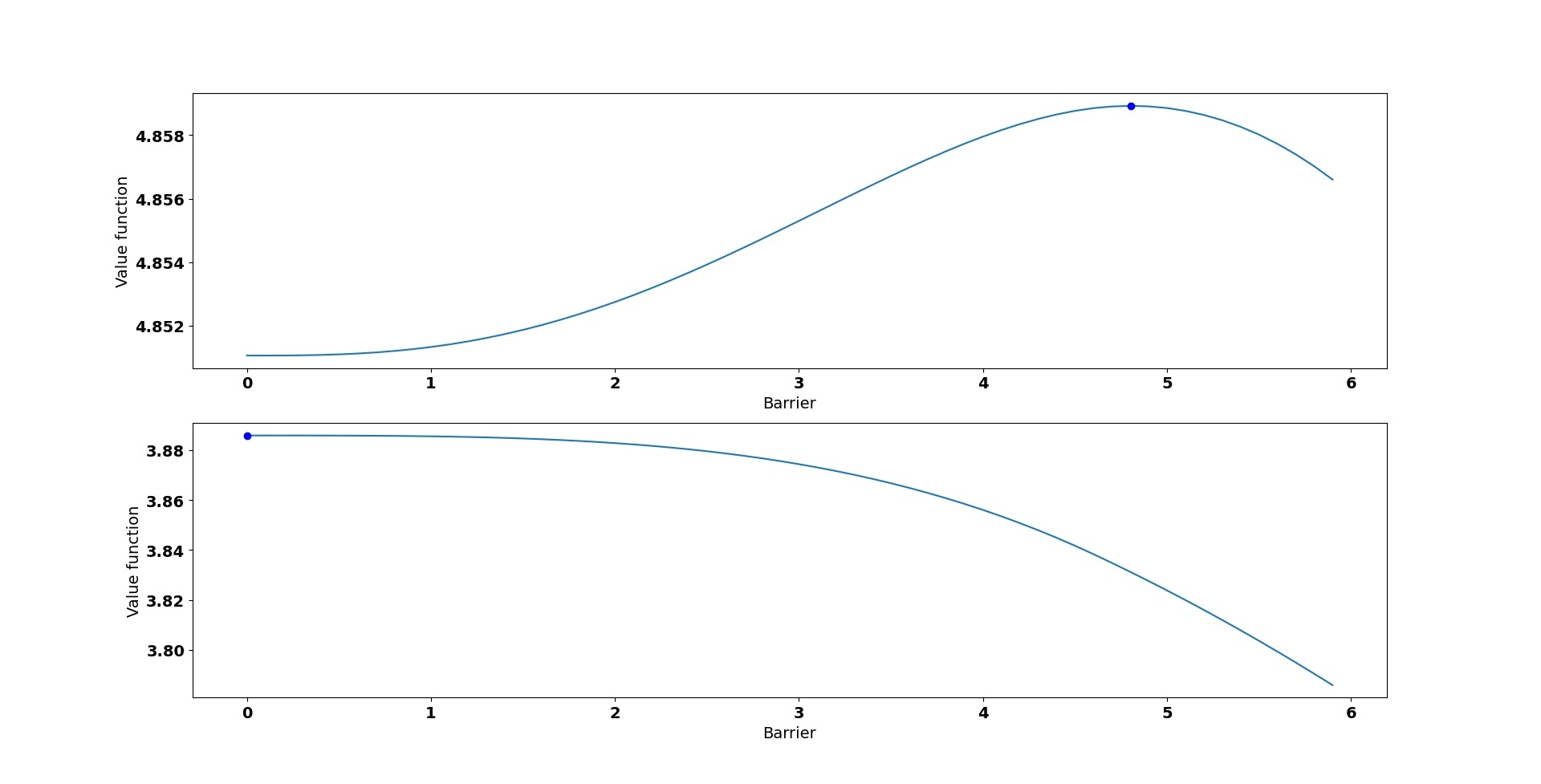
Figure 1. Value function of $\pi_{b}$ as a function of $b$. The dot indicates the value function at $b^{\ast}$ given by Equation (10). Top panel: $\mu=0.3$, $\sigma=4.5$, $K=0.1$, $q=0.025$ and $U_{0}=4.60$. Bottom panel: $\mu=0.3$, $\sigma=4.5$, $K=0.1$, $q=0.05$ and $U_{0}=4.60$.

Second, in Figure 2, we draw the value function for a (delayed) linear control strategy as a function of two variables: the barrier level $b$ and the parameter $K$. The curve on the surface identifies the value function corresonding to the optimal barrier $b^{\ast}$. For small values of $K$, $\mu K/q^{2}<\Delta$ and we see that the optimal barrier is $b^{\ast}=0$ while for values of $K$ such that $\mu K/q^{2}>\Delta$ we see that $b^{\ast}>0$.

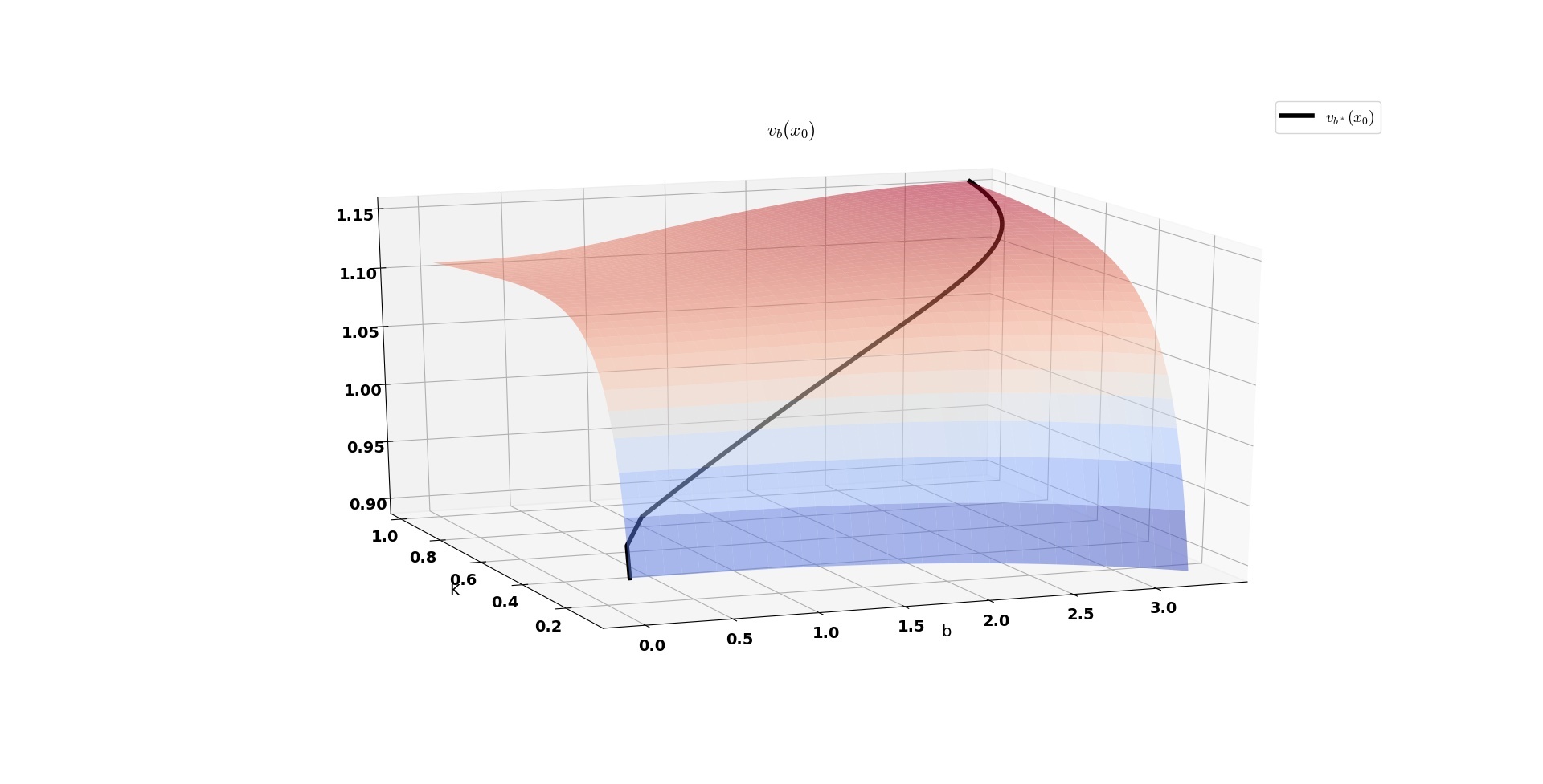
Figure 2. Value function of $\pi_{b}$ as a function of the variables $b$ and $K$. The curve is the value function of $\pi_{b^{\ast}}$. Parameters: $\mu=0.3$, $\sigma=2.5$, $q=0.07$ and $x_{0}=1$.

Finally, as alluded to in the introduction, when $K$ goes to infinity, one expects to recover de Finetti’s classical control problem, in which the optimal strategy is to pay out all surplus in excess of the barrier level $c^{\ast}$, as given by (4). Recall from Proposition 2.2 that the optimal level $b^{\ast}$ in our problem is always less than $c^{\ast}$. In Figure 3, we draw the value of the optimal barrier level $b^{\ast}$ as a function of $K$, i.e., $K\mapsto b^{\ast}(K)$. One can see that, for this set of parameters, the optimal barrier level $b^{\ast}(K)$ increases to $c^{\ast}$ as $K$ increases to infinity.

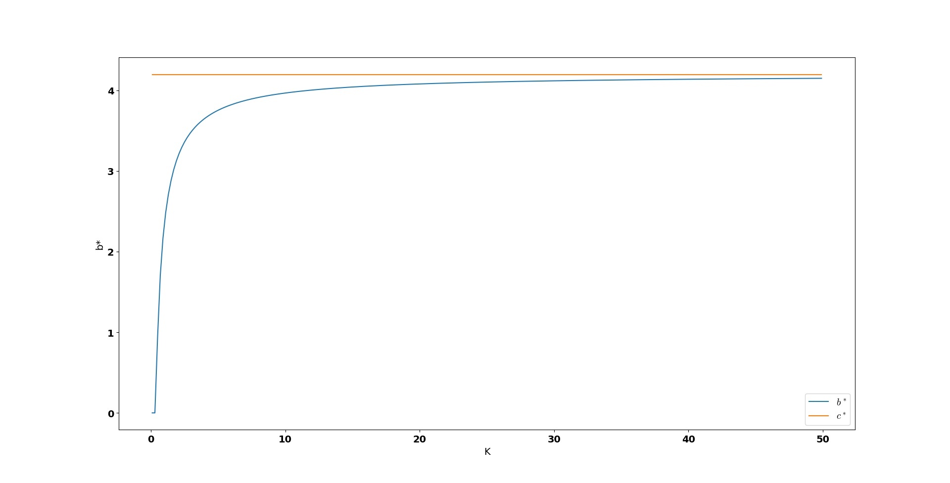
Figure 3. Optimal barrier level $b^{\ast}$ as a function of $K$. The red line corresponds to $c^{\ast}$. Parameters: $\mu=0.3$, $\sigma=4.5$, $q=0.07$ and $U_{0}=1$.

Appendix A Existence of the refracted diffusion process given by (2)

It is well known, thanks to Proposition 3.6 in Section 5.3 of [karatzas-shreve_1991], that Equation (2) has a weak solution. However, we can prove the existence of a strong solution by mimicking the proof of Lemma 12 in [Kyprianou/Loeffen_2010].

Fix an arbitrary $T>0$. For each $n\geq 1$, let $\{T^{n}_{i}\colon i=0,\dots,n\}$ be a sequence of partitions such that $T^{n}_{0}=0<T^{n}_{1}<\cdots<T^{n}_{n}=T$ and $\lim_{n\to\infty}\max_{1\leq i\leq n}|T^{n}_{i}-T^{n}_{i-1}|=0$. For $t\in[0,T]$, let $X_{t}=\mu t+\sigma W_{t}$ and, for each $n$, define $X^{n}_{t}=\mu t+\sigma W_{T^{n}_{i}}$, if $T^{n}_{i}\leq t<T^{n}_{i+1}$, for $i=0,1,\dots,n-1$. One can show that the sequence of processes $\{X^{n},n=1,2,\dots\}$ converges strongly to $X$, i.e.,

$$\lim_{n\to\infty}\sup_{t\in[0,T]}|X^{n}_{t}-X_{t}|=0$$

almost surely. Now, define the sequence of processes $\{U^{n},n=1,2,\dots\}$ by: for each $t\in[0,T]$, set

$$U^{n}_{t}=X^{n}_{t}-K\int_{0}^{t}U^{n}_{s}\mathbf{1}_{\{U^{n}_{s}>b\}}\mathrm{d}s.$$

Clearly, for each $n\geq 1$, $U^{n}$ is a well-defined process. Let us show that $\{U^{n},n=1,2,\dots\}$ is a strong Cauchy sequence and thus converges to a process $U$ such that

$$U_{t}=X_{t}-K\int_{0}^{t}U_{s}\mathbf{1}_{\{U_{s}>b\}}\mathrm{d}s.$$

Define, for all for $t\in[0,T]$, $\Delta^{n,m}X_{t}:=X^{n}_{t}-X^{m}_{t}$, $\Delta^{n,m}U_{t}:=U^{n}_{t}-U^{m}_{t}$ and

$$A^{n,m}_{t}:=\Delta^{n,m}U_{t}-\Delta^{n,m}X_{t}=-K\int_{0}^{t}\left(U^{n}_{s}\mathbf{1}_{\{U^{n}_{s}>b\}}-U^{m}_{s}\mathbf{1}_{\{U^{m}_{s}>b\}}\right)\mathrm{d}s.$$

Fix $\epsilon>0$. As $\{X^{n},n=1,2\dots\}$ converges strongly to $X$, there exists an integer $N_{\epsilon}$ such that: if $n,m>N_{\epsilon}$, then $\sup_{t\in[0,T]}|\Delta^{n,m}X_{t}|<\epsilon$. Let us show by contradiction that, for any $n,m>N_{\epsilon}$, we have $\sup_{t\in[0,T]}|A^{n,m}_{t}|<\epsilon$. Assume it is not verified. Then, from the continuity of $t\mapsto A^{n,m}_{t}$ and since $A^{n,m}_{0}=0$, there exists $s\in[0,T]$ such that $|A^{n,m}_{s}|=\epsilon$ and such that, for any sufficiently small $\delta>0$, there exists $r_{s}\in[s,s+\delta)$ such that $|A^{n,m}_{r_{s}}|>\epsilon$. Assume that $A^{n,m}_{s}=\epsilon<A^{n,m}_{r_{s}}$.

Since, for all $t\in[0,T]$, $\Delta^{n,m}X_{t}\in(-\epsilon,\epsilon)$ and $A^{n,m}_{t}=\Delta^{n,m}U_{t}-\Delta^{n,m}X_{t}$, then $\Delta^{n,m}U_{s}>0$ and there exists $\delta>0$ such that $\Delta^{n,m}U_{r}>0$ for all $r\in[s,s+\delta)$. Consequently, for each $r\in[s,s+\delta)$,

$$A^{n,m}_{r}-A^{n,m}_{s}=-K\int_{s}^{r}\left(U^{n}_{v}\mathbf{1}_{\{U^{m}_{v}>b\}}-U^{m}_{v}\mathbf{1}_{\{U^{m}_{v}>b\}}\right)\mathrm{d}v<0.$$

This is a contradiction. A similar argument can be used for the case $A^{n,m}_{s}=-\epsilon$.

In conclusion, for any $n,m>N_{\epsilon}$, we have $\sup_{t\in[0,T]}|A^{n,m}_{t}|<\epsilon$ and thus, by the triangle inequality, we have $\sup_{t\in[0,T]}|\Delta^{n,m}U_{t}|<2\epsilon$.

Appendix B Differential equations and analytical properties

It is well known (and easy to verify) that $W^{(q)}$, defined in (7), is a solution to the following ordinary differential equation (ODE):

$$\frac{\sigma^{2}}{2}f^{\prime\prime}(x)+\mu f^{\prime}(x)-qf(x)=0,\quad x>0.$$

Hence, for $x>0$, we have

$$W^{(q)\prime\prime}(x)=\frac{2}{\sigma^{2}}\left(qW^{(q)}(x)-\mu W^{(q)\prime}(x)\right).$$

We are also interested in the following non-homogeneous ODE:

$$\frac{\sigma^{2}}{2}f^{\prime\prime}(x)+\left(\mu-Kx\right)f^{\prime}(x)-qf(x)+Kx=0,\quad x>0.$$ (14)

We are looking for a solution of the form $f(x)=f_{p}(x)+f_{h}(x)$, where $f_{p}$ is a particular solution and where $f_{h}$ is a solution of the homogeneous version of (14), that is

$$\frac{\sigma^{2}}{2}f^{\prime\prime}(x)+\left(\mu-Kx\right)f^{\prime}(x)-qf(x)=0,\quad x>0.$$ (15)

On one hand, it is easy to verify that

$$f_{p}(x)=\frac{K}{q+K}\left(x+\frac{\mu}{q}\right)$$

is a solution to the ODE in (14). On the other hand, from [borodin-salminen_2002], it is known that, for $\lambda>0$,

$$b^{2}f^{\prime\prime}(x)-xf^{\prime}(x)-\lambda f(x)=0,\quad x\in\mathbb{R},$$

admits

$$\psi_{\lambda}(x)=\mathrm{e}^{x^{2}/4b^{2}}\mathrm{D}_{-\lambda}\left(-x/b\right)\quad\text{and}\quad\varphi_{\lambda}(x)=\mathrm{e}^{x^{2}/4b^{2}}\mathrm{D}_{-\lambda}\left(x/b\right),$$

as its increasing solution and its decreasing solution, respectively, where $\mathrm{D}_{-\lambda}$ is the parabolic cylinder function defined by: for $x\in\mathbb{R}$,

$$\mathrm{D}_{-\lambda}(x)=\frac{1}{\Gamma(\lambda)}\mathrm{e}^{-x^{2}/4}\int_{0}^{\infty}t^{\lambda-1}\mathrm{e}^{-xt-t^{2}/2}\mathrm{d}t.$$

Since $H_{K}^{(q)}(x)=\varphi_{q/K}\left(\left(x-\mu/K\right)\sqrt{2K}\right)$, as defined in (9), we deduce that $H_{K}^{(q)}$ is a solution to the homogeneous ODE in (15). Hence, for $x>0$, we have

$$H_{K}^{(q)\prime\prime}(x)=\frac{2}{\sigma^{2}}\left(\left(Kx-\mu\right)H_{K}^{(q)\prime}(x)+qH_{K}^{(q)}(x)\right).$$

Finally, we have that

$$f(x)=\frac{K}{q+K}\left(x+\frac{\mu}{q}\right)+D_{b}H_{K}^{(q)}(x)$$

is a solution to the non-homogeneous ODE in (14).