Abstract

A range of methods with suitable inductive biases exist to learn interpretable object-centric representations of images without supervision. However, these are largely restricted to visually simple images; robust object discovery in real-world sensory datasets remains elusive. To increase the understanding of such inductive biases, we empirically investigate the role of “reconstruction bottlenecks” for scene decomposition in genesis, a recent vae-based model. We show such bottlenecks determine reconstruction and segmentation quality and critically influence model behaviour.

1 Introduction

Interest in unsupervised object-centric generative models (Burgess et al., 2019; Greff et al., 2019; Engelcke et al., 2020) is driven by the premise of increased sample efficiency and generalisation for tasks that involve interaction with objects (e.g. Watters et al., 2019a). While these methods exhibit suitable inductive biases to identify interpretable components, understanding of these biases is limited and their application to more complex real-world datasets is an unresolved challenge (e.g. Greff et al., 2019).

We posit that enhancing the understanding of inductive biases for scene decomposition can facilitate the development of better object-centric generative models, both on current and more difficult datasets. Specifically, we argue that methods based on variational autoencoders (vaes) (Kingma & Welling, 2014; Rezende et al., 2014) that learn object-centric representation by learning to reconstruct input images (e.g. Burgess et al., 2019; Greff et al., 2019; Engelcke et al., 2020) feature what we call reconstruction bottlenecks that induce decomposition by prohibiting the model from reconstructing an image as a single component. Therefore, we present an empirical investigation of this mechanism as the reconstruction bottleneck is traversed and we examine how it impacts reconstruction and segmentation quality.​

To do this, we conduct experiments with genesis (Engelcke et al., 2020), a recently developed model for unsupervised segmentation and component-wise generation. genesis features two sets of VAEs: mask VAEs model pixel-wise segmentation masks and component VAEs reconstruct object appearances. Notably, the model features an asymmetric architecture; the mask VAEs feature mirrored convolutional and deconvolutional layers, but the component VAEs use spatial broadcast decoders (sbds) (Watters et al., 2019b). These encourage latent disentanglement and act—as we argue—as a reconstruction bottleneck. We thus examine model behaviour when varying the latent dimensions before the object appearance decoder with the original architecture as well as with a modified, symmetric architecture.

Experiments are conducted on Multi-dSprites (Burgess et al., 2019), ShapeStacks (Groth et al., 2018), and ObjectsRoom (Kabra et al., 2019). The original, asymmetric genesis architecture achieves similar segmentation performance across a broad range of latent dimensions and only degrades when it is very small. We argue the sbd-architecture inhibits the learning of good reconstructions and thus serves as the effective bottleneck when the latent dimensionality is large. For the symmetric architecture with matched encoders and decoders, however, good segmentation is only achieved in a very narrow window of suitably small latent dimensions before the object appearance decoder.

An intricate interplay between segmentation and reconstruction is observed: If the bottleneck is too narrow, segmentation and reconstruction degrade. If it is too wide, reconstruction is reasonable but the model collapses to a single component and no useful segmentation is learned. While these observations are intuitive for experienced practitioners, we found that—to the best of our knowledge—an extensive formal treatment has been missing in the literature. They also provide insight into the suitability of sbds for object-centric models trained on these types of datasets. We believe this provides useful guidance for researchers and practitioners, both established and new to the field, and hope this work encourages a more open discussion of the design process of object-centric models.​

2 Related Work

Object-centric generative models can be categorised according to their training objective: (1) reconstruction-based (Huang & Murphy, 2015; Eslami et al., 2016; Greff et al., 2016; 2017; 2019; van Steenkiste et al., 2018a; Kosiorek et al., 2018; 2019; Crawford & Pineau, 2019; Burgess et al., 2019; von Kügelgen et al., 2020; Kossen et al., 2020; Lin et al., 2020; Jiang et al., 2020; Engelcke et al., 2020) and (2) adversarial (van Steenkiste et al., 2018b; Chen et al., 2019; Bielski & Favaro, 2019; Arandjelović & Zisserman, 2019; Azadi et al., 2019; Nguyen-Phuoc et al., 2020). A discriminative approach for learning object-centric representations has also been proposed (Kipf et al., 2020).

While this work focuses on the reconstruction-based model in Engelcke et al. (2020), we argue most methods of this type feature reconstruction bottlenecks for inducing scene decomposition. For example, Burgess et al. (2019) also use a flexible segmentation network and a less expressive component appearance network with an sbd. While Greff et al. (2019) use the same network for segmentation and appearance, they also use an sbd with limited expressiveness for decoding. Similarly, in methods that use spatial transformers (Jaderberg et al., 2015) instead of segmentation masks for distinguishing objects (e.g. Huang & Murphy, 2015; Eslami et al., 2016; Kosiorek et al., 2018; Crawford & Pineau, 2019; Jiang et al., 2020), the dimensions of the transformer sampling grid constitute a reconstruction bottleneck. We therefore conjecture the findings in this work will also apply to a range of other model formulations.

3 Background: GENESIS

generative scene inference and sampling (genesis) (Engelcke et al., 2020) is a vae which encodes an image $\mathbf{x}\in\mathbb{R}^{H\times W\times C}$ into a set of mask variables $\mathbf{z}^{m}_{k}$ and a set of component variables $\mathbf{z}^{c}_{k}$ where $k\in 1,\dots,K$ and $K$ is the maximum number of image components. The mask variables are decoded into a set of normalised mixture probabilities, or segmentation masks, $\pi_{k}$ and the component variables are decoded into a parameterised set of generated component appearances $p_{\theta}\left(\mathbf{x}_{k}\mid\mathbf{z}^{c}_{k}\right)$. Together, these parameterise a spatial Gaussian mixture model (sgmm) for the image likelihood (see Greff et al., 2017):

$$p\left(\mathbf{x}\mid\mathbf{z}^{m}_{1:K},\mathbf{z}^{c}_{1:K}\right)=\sum_{k=1}^{K}\pi_{k}\,p_{\theta}\left(\mathbf{x}_{k}\mid\mathbf{z}^{c}_{k}\right)\,.$$ (1)

The mask variables are inferred in an autoregressive fashion and decoded in parallel. Individual masks are subsequently concatenated with the image to infer the component latents. This forward pass through the model is illustrated in Fig. 1.

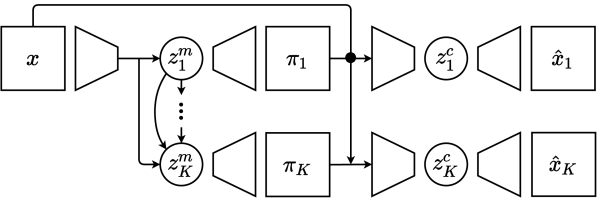
Figure 1: genesis architecture (Engelcke et al., 2020). Given an image $\mathbf{x}$, mask variables $\mathbf{z}^{m}_{k}$ and component variables $\mathbf{z}^{c}_{k}$ encode mixture probabilities $\pi_{k}$ and component appearances $p_{\theta}\left(\mathbf{x}_{k}\mid\mathbf{z}^{c}_{k}\right)$.

Generative model  The generative model can be written as:

$$p_{\theta}\left(\mathbf{x}\right)=\iint p_{\theta}\left(\mathbf{x}\mid\mathbf{z}^{c},\mathbf{z}^{m}\right)p_{\theta}\left(\mathbf{z}^{c}\mid\mathbf{z}^{m}\right)p_{\theta}\left(\mathbf{z}^{m}\right)\,\mathrm{d}\mathbf{z}^{m}\,\mathrm{d}\mathbf{z}^{c}\,,$$ (2)

where component subscripts are not shown for brevity. The prior distributions over latent variables factorise as:

$$p_{\theta}\left(\mathbf{z}_{1:K}^{m}\right)=\prod_{k=1}^{K}p_{\theta}\left(\mathbf{z}^{m}_{k}\mid\mathbf{z}^{m}_{1:k-1}\right)\,,$$ (3)

$$p_{\theta}\left(\mathbf{z}^{c}_{1:K}\mid\mathbf{z}^{m}_{1:K}\right)=\prod_{k=1}^{K}p_{\theta}\left(\mathbf{z}^{c}_{k}\mid\mathbf{z}^{m}_{k}\right)\,.$$ (4)

Inference model  The inference model can be written as:

$$q_{\phi}\left(\mathbf{z}_{1:K}^{c},\mathbf{z}_{1:K}^{m}\mid\mathbf{x}\right)=q_{\phi}\left(\mathbf{z}_{1:K}^{m}\mid\mathbf{x}\right)\,q_{\phi}\left(\mathbf{z}_{1:K}^{c}\mid\mathbf{x},\mathbf{z}_{1:K}^{m}\right)\,,$$ (5)

The posterior distributions over latent variables factorise as:

$$q_{\phi}\left(\mathbf{z}_{1:K}^{m}\mid\mathbf{x}\right)=\prod_{k=1}^{K}q_{\phi}\left(\mathbf{z}_{k}^{m}\mid\mathbf{x},\mathbf{z}_{1:k-1}^{m}\right)\,,$$ (6)

$$q_{\phi}\left(\mathbf{z}_{1:K}^{c}\mid\mathbf{x},\mathbf{z}_{1:K}^{m}\right)=\prod_{k=1}^{K}q_{\phi}\left(\mathbf{z}_{k}^{c}\mid\mathbf{x},\mathbf{z}_{1:k}^{m}\right)\,.$$ (7)

Implementation  All prior and conditional distributions are diagonal Gaussians. The distributions in Eq. 4 and Eq. 7 are parameterised by feedforward networks and the autoregressive distributions in Eq. 3 and Eq. 6 are parameterised by RNNs. The mask sub-network uses gated (de-)convolutions (Dauphin et al., 2017; Berg et al., 2018) with batch normalisation (bn) (Ioffe & Szegedy, 2015) and the component sub-network has an architecture similar to Burgess et al. (2019) with an sbd and ELUs (Clevert et al., 2016) instead of ReLUs (Glorot et al., 2011). This architecture asymmetry is at the focus of the experiments in this work. Finally, the model is trained by optimising the Generalised elbo with Constrained Optimisation (geco) objective from Rezende & Viola (2018). We refer the reader to Engelcke et al. (2020) for further details.

4 Experiments

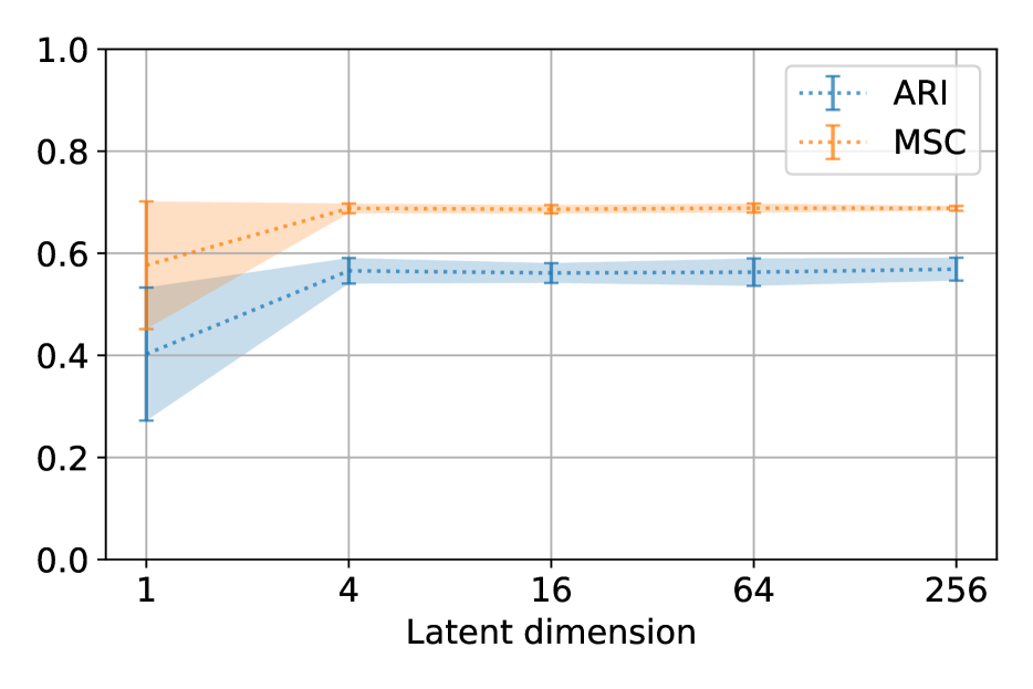
(a) Multi-dSprites

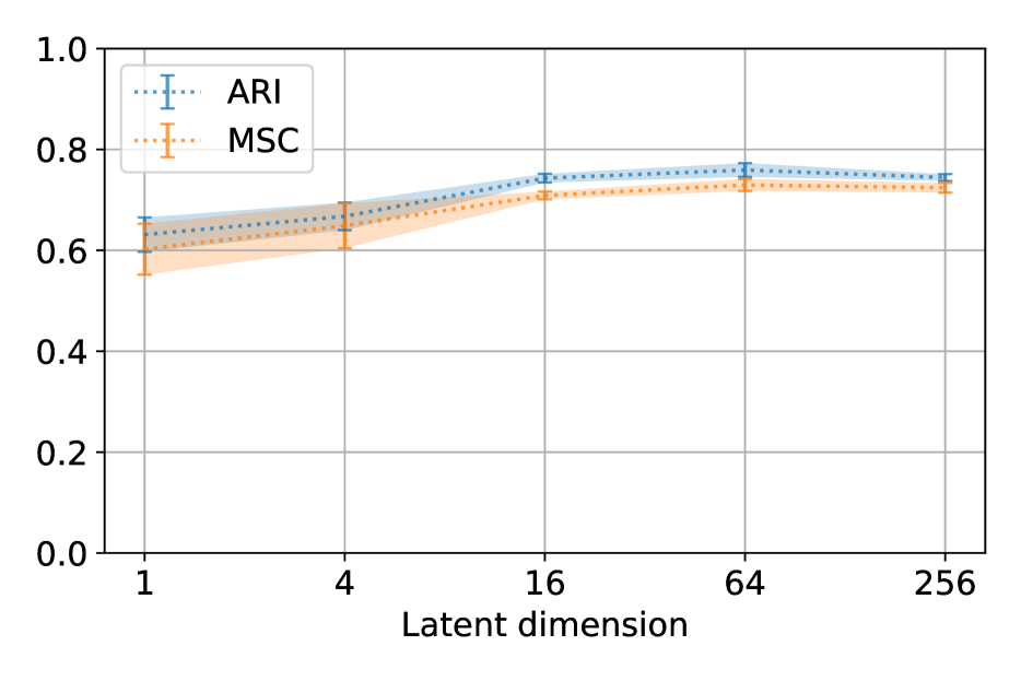
(b) ShapeStacks

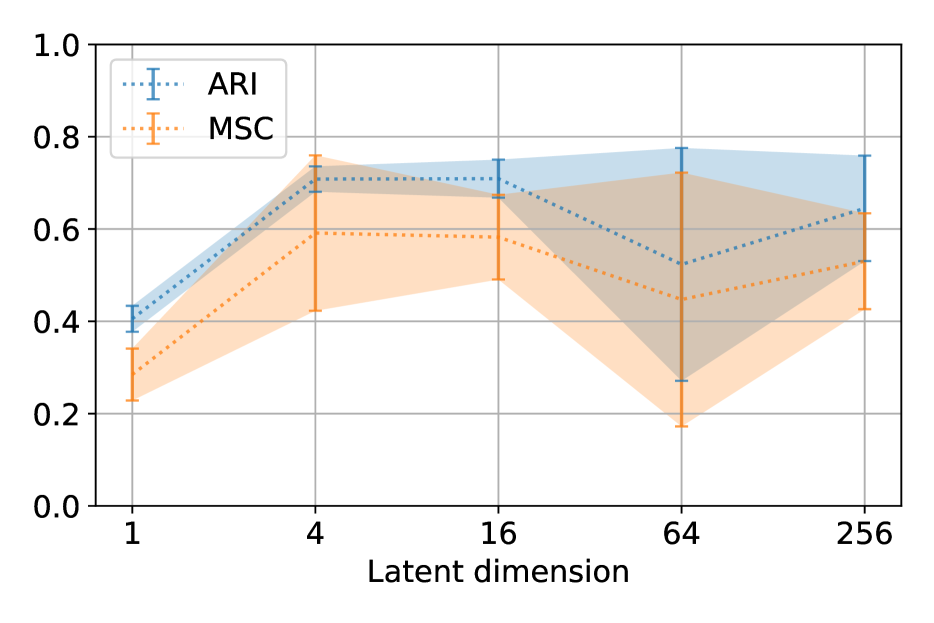
(c) ObjectsRoom

Figure 2: Segmentation performance for the original—asymmetric—genesis architecture as the component latent dimension is varied. Decomposition occurs throughout the entire range for all three datasets, but performance drops when the latent dimension is very small.

Datasets  Experiments are conducted on Multi-dSprites, (Burgess et al., 2019), ShapeStacks (Groth et al., 2018), and ObjectsRoom (Kabra et al., 2019). A withheld validation set is used for obtaining segmentation metrics. We follow Engelcke et al. (2020) for Multi-dSprites and ShapeStacks. For ObjectsRoom, we withhold 20,000 images from the training set in Kabra et al. (2019) for evaluation.

Setup  We perform experiments with different latent dimensions in the component vae for both the original, asymmetric architecture from Engelcke et al. (2020) (Sec. 4.1) and a modified, symmetric architecture (Sec. 4.2). The asymmetric architecture has a spatial broadcast decoder (sbd) in the component vae and gated (de-)convolutions and batch normalisation in the mask vae; experiments are conducted with latent dimensions of $\{1,4,16,64,256\}$. For the symmetric architecture, the same encoder and decoder with gated (de-)convolutions and batch normalisation as used in the mask vae are also used in the component vae. Here, we observed that decomposition is only achieved for smaller latent dimensions and therefore modified the range to $\{1,2,4,8,16\}$ to increase the resolution in the hyperparameter subspace where interesting behaviour occurs. Experiments use the implementation from Engelcke et al. (2020) and identical optimisation hyperparameters.

Metrics  Segmentation performance is quantified with the Adjusted Rand Index (ari) and the Mean Segmentation Covering (msc), on 300 images not seen during training (see Greff et al., 2019; Engelcke et al., 2020). We report the means and standard deviations obtained with three different random seeds. Larger values are better.

Compute  Training a single model takes on average around two days on an NVIDIA Titan RTX card. The results presented in this work amount to training a total of 90 individual models, corresponding to ca. 180 GPU days.

Further details and results are included in the appendix.

4.1 Asymmetric architecture

Segmentation performance on the three datasets is shown in Fig. 2. It can be observed that the models decompose the images across the whole range of latent dimensions. Separately, we also train the component reconstruction architecture as a vanilla sbd-vae for different latent dimensions, recording either the number of iterations required to reach the geco reconstruction goal or the final moving average of the reconstruction error (Tab. 1). The sbd-vae never reaches the geco goal on its own and the reconstruction error does not further decrease for latent dimensions larger than 32. We conclude that the structure of the sbd slows down the minimisation of the reconstruction loss and that in the asymmetric genesis architecture it is this structure—rather than latent dimensionality—which acts as the effective bottleneck, at least when the latent dimension is large. This therefore prevents the models to collapse to a trivial solution where images are reconstructed as a single component. Finally, segmentation performance slightly drops when the latent dimension is very small. We conjecture that this is caused by the lack of detail in lower quality reconstructions.

Table 1: sbd-vae training iterations needed to reach the geco reconstruction goal of 0.5655. If the goal is not reached within 500k iterations, the final moving average error is reported instead.

	Multi-dSprites		ShapeStacks		ObjectsRoom
Latent	Goal	500k	Goal	500k	Goal	500k
dim	iter	err	iter	err	iter	err
1	-	0.5885	-	0.5852	-	0.6064
2	-	0.5820	-	0.5819	-	0.5921
4	-	0.5763	-	0.5785	-	0.5820
8	-	0.5730	-	0.5754	-	0.5767
16	-	0.5697	-	0.5730	-	0.5715
32	-	0.5676	-	0.5709	-	0.5703
64	-	0.5675	-	0.5712	-	0.5698
128	-	0.5676	-	0.5715	-	0.5700
256	-	0.5674	-	0.5710	-	0.5700

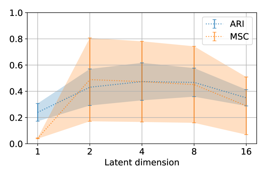
(a) Multi-dSprites

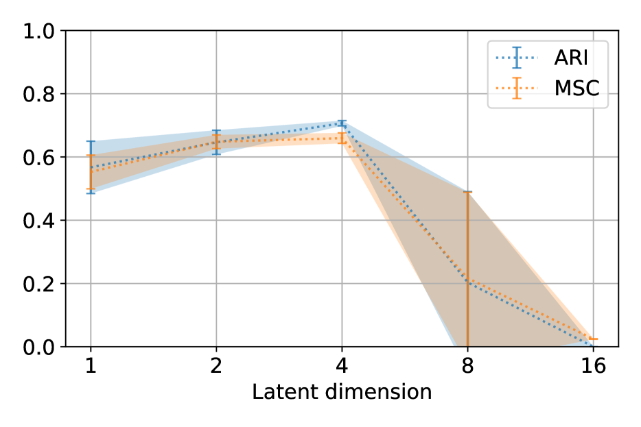
(b) ShapeStacks

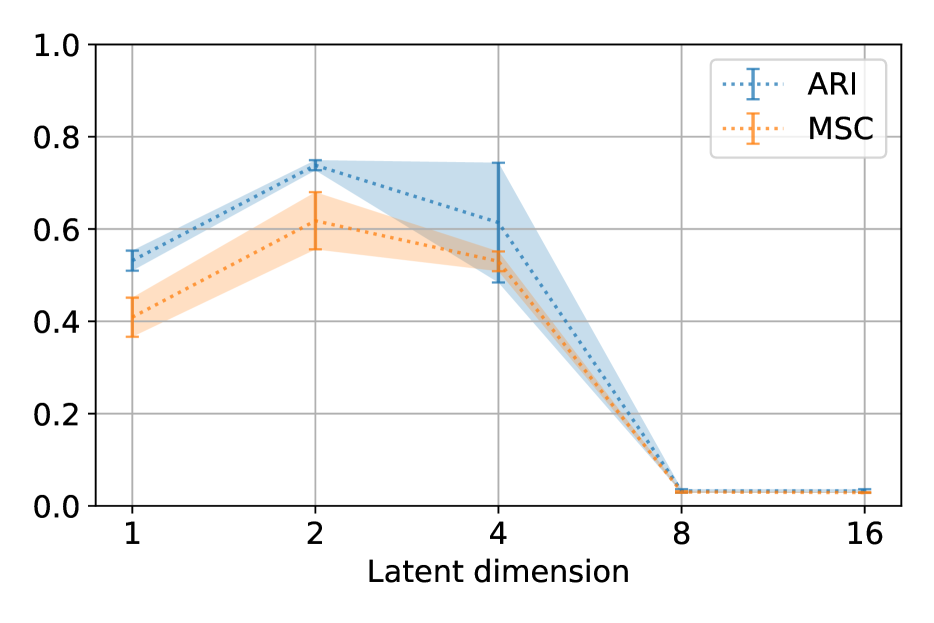
(c) ObjectsRoom

Figure 3: Segmentation performance for the modified—symmetric—genesis architecture as the component latent dimension is varied. Decomposition only occurs in a small range of latent dimensions and performance drops when the latent dimension is small.

4.2 Symmetric architecture

Segmentation performance is shown in Fig. 3. It can be seen that if the component latent dimension is too large, the models consistently collapse to a single component. As shown in the appendix, this does not necessarily adversely affect reconstruction quality: the modified component vae is expressive enough to produce good reconstructions without decomposition. For smaller latents, however, there is a range where the models learn to segment the images into object-like components. Similar to before, segmentation quality deteriorates when the latent dimension becomes very small. We argue that the difference in behaviour here is due to the modified architecture being sufficiently expressive so that the latent dimension is the effective reconstruction bottleneck, hence exhibiting a critical influence on model behaviour. We train the component architecture as a vanilla dc-vae for different latent dimensions (Tab. 2). The range of latents where genesis learns to decompose images somewhat correlates with the range where the final dc-vae reconstruction error is relatively far away from the geco goal, i.e. $>0.5670$ for latent dimensions in the interval $[1,8]$.

Table 2: dc-vae training iterations needed to reach the geco reconstruction goal of 0.5655. If the goal is not reached within 500k iterations, the final moving average error is reported instead.

	Multi-dSprites		ShapeStacks		ObjectsRoom
Latent	Goal	500k	Goal	500k	Goal	500k
dim	iter	err	iter	err	iter	err
1	-	0.6008	-	0.5820	-	0.6082
2	-	0.5808	-	0.5766	-	0.5904
4	-	0.5753	-	0.5726	-	0.5825
8	-	0.5697	-	0.5683	-	0.5733
16	-	0.5660	246k	-	-	0.5668
32	079k	-	025k	-	061k	-
64	021k	-	009k	-	016k	-
128	010k	-	006k	-	007k	-
256	008k	-	005k	-	006k	-

5 Discussion

This work performs an empirical investigation into the role of “reconstruction bottlenecks” in a vae-based unsupervised object-centric generative model. An intricate interplay between reconstruction and image decomposition occurs: if the effective bottleneck in the part of the model that reconstructs individual components is too narrow, reconstruction and segmentation quality suffer. Conversely, if the effective bottleneck is too wide, the models do not learn to decompose images and instead collapse to a trivial solution. Depending on design decisions made by the practitioner, this effective bottleneck can either be controlled by the latent dimensionality or the architecture.

We believe these results provide valuable insights into the inductive biases for these types of models and provide useful guidance for researchers and practitioners. It would be interesting to examine these properties with other spatial mixture models (e.g. Burgess et al., 2019; Greff et al., 2019) as well as spatial transformer models (e.g. Eslami et al., 2016; Jiang et al., 2020). Another possible direction could be to investigate the relationship between optimal bottleneck size and dataset complexity as well as utilising vanilla vae behaviour to predict decomposition quality when the identical vae is used for modelling components in an object-centric model.

Reconstruction bottlenecks appear to be a sufficient mechanism for learning object-centric representations when scene components have comparable visual complexity. It would be interesting to investigate how this approach fares for datasets where texture variance is more variable across scene components; for example, in a real-world image of an indoor room, the walls are often uniformly coloured whereas other components, e.g. furniture, can have arbitrarily complex appearances. Leveraging additional inductive biases such as motion (Kosiorek et al., 2018; Jiang et al., 2020) or depth and geometry (Byravan & Fox, 2017; Nguyen-Phuoc et al., 2020) might be beneficial for this.

Appendix A Component vae architecture details

A.1 Asymmetric genesis and sbd-vae

This architecture corresponds to the original genesis formulation. It is used for the results in Fig. 2, Fig. 4, and Fig. 6 as well as the results for the corresponding vanilla sbd-vae in Tab. 1. The latter is equivalent to training asymmetric genesis with only a single component.

Table 3: Original vae encoder

Input spatial dim	Input channels	Output channels	Kernel size	Stride	Layer type	Activation
64	3 + 1	32	3$\times$3	2	Conv	ELU
32	32	32	3$\times$3	2	Conv	ELU
16	32	64	3$\times$3	2	Conv	ELU
8	64	64	3$\times$3	2	Conv	ELU
-	4$\times$4$\times$64	256	-	-	FC	ELU
-	256	2$\times$latent dim	-	-	FC	-

Table 4: Original vae decoder

Input spatial dim	Input channels	Output channels	Kernel size	Stride	Layer type	Activation
-	latent dim	latent dim + 2	-	-	Broadcast	-
72	latent dim + 2	32	3$\times$3	1	Conv	ELU
70	32	32	3$\times$3	1	Conv	ELU
68	32	32	3$\times$3	1	Conv	ELU
66	32	32	3$\times$3	1	Conv	ELU
64	32	3	1$\times$1	1	Conv	-

A.2 Symmetric genesis and dc-vae

This architecture corresponds to the modified genesis formulation. It is used for the results in Fig. 3, Fig. 5, and Fig. 7 as well as the results for the corresponding vanilla dc-vae in Tab. 2. The latter is equivalent to training symmetric genesis with only a single component. It encoder and decoder are very similar to the corresponding mask vae modules in genesis. Note that the GLU non-linearities half the number of output channels.

Table 5: Modified, higher capacity vae encoder

Input spatial dim	Input channels	Output channels	Kernel size	Stride	Layer type	Activation
64	3 + 1	64	5$\times$5	1	Conv	BN-GLU
64	32	32	5$\times$5	2	Conv	BN-GLU
32	32	128	5$\times$5	1	Conv	BN-GLU
32	64	128	5$\times$5	2	Conv	BN-GLU
16	64	128	5$\times$5	1	Conv	BN-GLU
-	16$\times$16$\times$64	4$\times$latent dim	-	-	FC	GLU

Table 6: Modified, higher capacity vae decoder

Input spatial dim	Input channels	Output channels	Kernel size	Stride	Layer type	Activation
-	latent dim	16$\times$16$\times$128	-	-	FC	GLU
16	64	128	5$\times$5	1	Deconv	BN-GLU
16	64	64	5$\times$5	2	Deconv	BN-GLU
32	32	64	5$\times$5	1	Deconv	BN-GLU
32	32	64	5$\times$5	2	Deconv	BN-GLU
64	32	64	5$\times$5	1	Deconv	BN-GLU
64	32	3	1$\times$1	1	Conv	-

Appendix B Reconstruction error

B.1 Asymmetric architecture

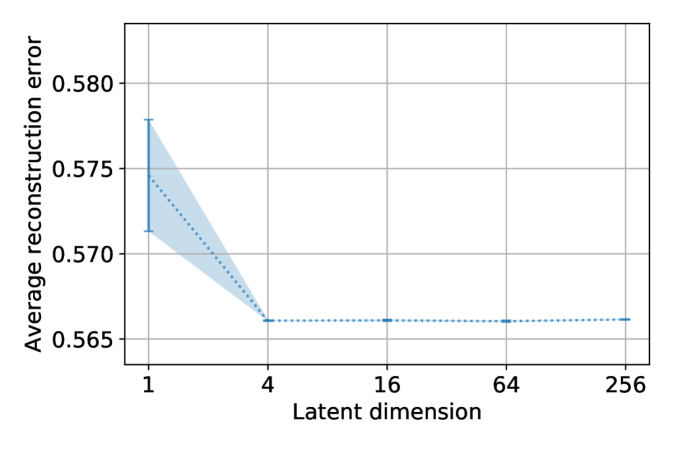
(a) Multi-dSprites

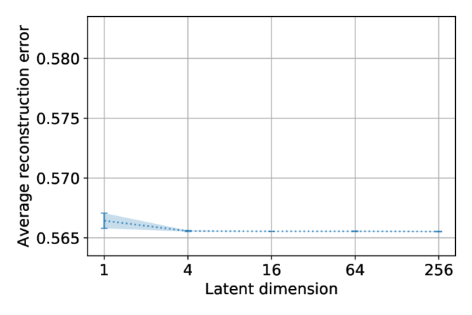
(b) ShapeStacks

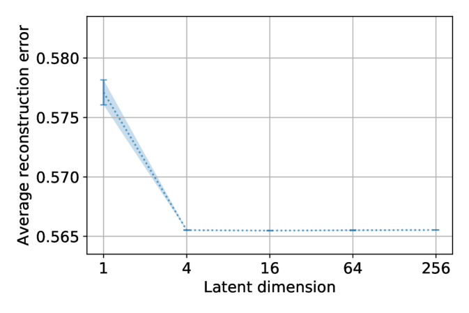
(c) ObjectsRoom

Figure 4: The average reconstruction error on the validation set is fairly constant for sufficiently large latent dimensions and only degrades when a single latent is used.

B.2 Symmetric architecture

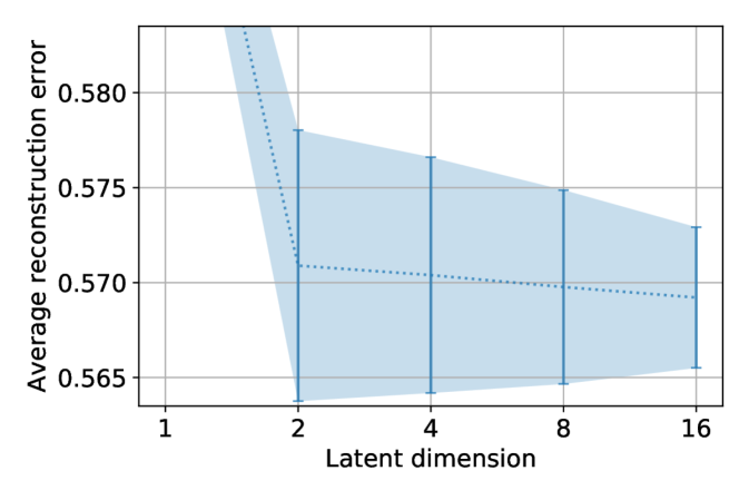
(a) Multi-dSprites

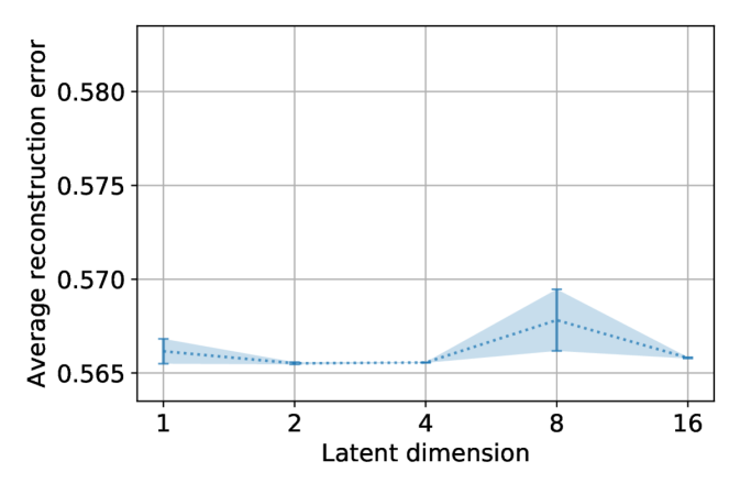
(b) ShapeStacks

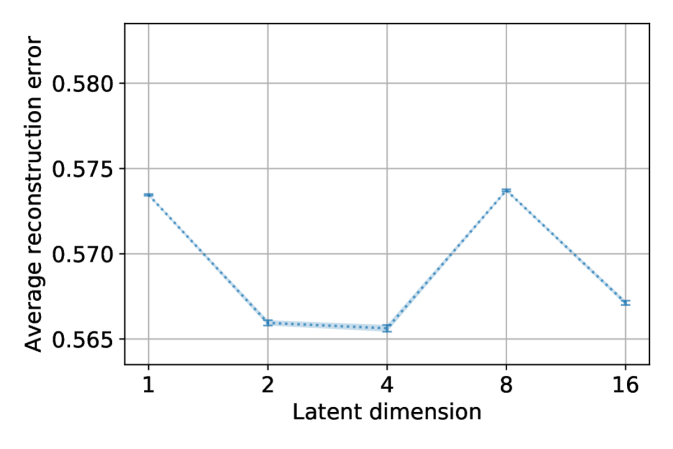
(c) ObjectsRoom

Figure 5: Average reconstruction error on the validation set is less stable than for the asymmetric architecture, but also degrades when only a single latent is used.

Appendix C Qualitative results

C.1 Asymmetric architecture

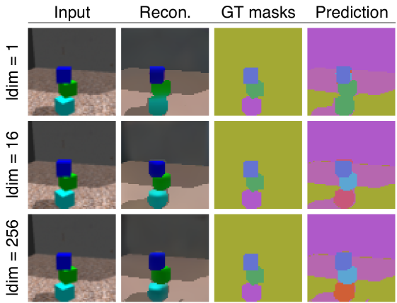
Figure 6: Qualitative segmentation performance with the original, asymmetric architecture on ShapeStacks for three different latent dimensions. Reconstruction and segmentation deteriorate slightly when only a single latent dimension is used.

C.2 Symmetric architecture

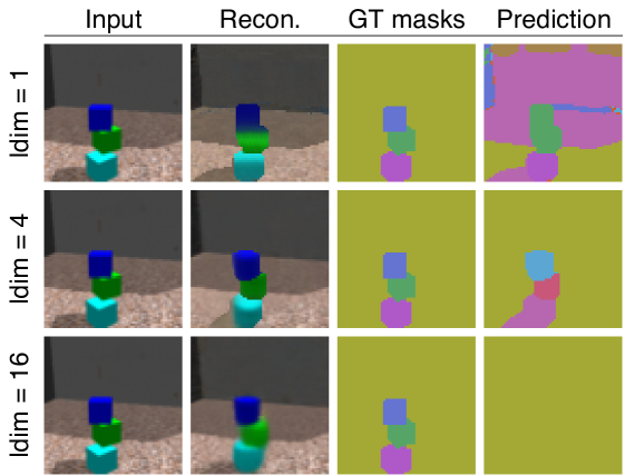
Figure 7: Qualitative segmentation performance with the modified, symmetric architecture on ShapeStacks for three different latent dimensions. Reconstruction and segmentation deteriorate when the latent dimension is too small. When the latent dimension is too large, segmentation collapses to a single component.

References

- Arandjelović & Zisserman (2019) Arandjelović, R. and Zisserman, A. Object Discovery with a Copy-Pasting GAN. arXiv preprint arXiv:1905.11369, 2019.
- Azadi et al. (2019) Azadi, S., Pathak, D., Ebrahimi, S., and Darrell, T. Compositional GAN: Learning Image-Conditional Binary Composition. arXiv preprint arXiv:1807.07560, 2019.
- Berg et al. (2018) Berg, R. v. d., Hasenclever, L., Tomczak, J. M., and Welling, M. Sylvester Normalizing Flows for Variational Inference. Conference on Uncertainty in Artificial Intelligence (UAI), 2018.
- Bielski & Favaro (2019) Bielski, A. and Favaro, P. Emergence of Object Segmentation in Perturbed Generative Models. arXiv preprint arXiv:1905.12663, 2019.
- Burgess et al. (2019) Burgess, C. P., Matthey, L., Watters, N., Kabra, R., Higgins, I., Botvinick, M., and Lerchner, A. MONet: Unsupervised Scene Decomposition and Representation. arXiv preprint arXiv:1901.11390, 2019.
- Byravan & Fox (2017) Byravan, A. and Fox, D. Se3-nets: Learning rigid body motion using deep neural networks. IEEE International Conference on Robotics and Automation (ICRA), 2017.
- Chen et al. (2019) Chen, M., Artières, T., and Denoyer, L. Unsupervised Object Segmentation by Redrawing. arXiv preprint arXiv:1905.13539, 2019.
- Clevert et al. (2016) Clevert, D.-A., Unterthiner, T., and Hochreiter, S. Fast and Accurate Deep Network Learning by Exponential Linear Units (ELUs). International Conference on Learning Representations (ICLR), 2016.
- Crawford & Pineau (2019) Crawford, E. and Pineau, J. Spatially Invariant Unsupervised Object Detection with Convolutional Neural Networks. AAAI Conference on Artificial Intelligence, 2019.
- Dauphin et al. (2017) Dauphin, Y. N., Fan, A., Auli, M., and Grangier, D. Language Modeling with Gated Convolutional Networks. International Conference on Machine Learning (ICML), 2017.
- Engelcke et al. (2020) Engelcke, M., Kosiorek, A. R., Parker Jones, O., and Posner, I. GENESIS: Generative Scene Inference and Sampling with Object-Centric Latent Representations. International Conference on Learning Representations (ICLR), 2020.
- Eslami et al. (2016) Eslami, S. A., Heess, N., Weber, T., Tassa, Y., Szepesvari, D., Hinton, G. E., et al. Attend, Infer, Repeat: Fast Scene Understanding with Generative Models. Advances in Neural Information Processing Systems (NeurIPS), 2016.
- Glorot et al. (2011) Glorot, X., Bordes, A., and Bengio, Y. Deep Sparse Rectifier Neural Networks. International Conference on Artificial Intelligence and Statistics (AISTATS), 2011.
- Greff et al. (2016) Greff, K., Rasmus, A., Berglund, M., Hao, T., Valpola, H., and Schmidhuber, J. Tagger: Deep Unsupervised Perceptual Grouping. Advances in Neural Information Processing Systems (NeurIPS), 2016.
- Greff et al. (2017) Greff, K., van Steenkiste, S., and Schmidhuber, J. Neural Expectation Maximization. Advances in Neural Information Processing Systems (NeurIPS), 2017.
- Greff et al. (2019) Greff, K., Kaufmann, R. L., Kabra, R., Watters, N., Burgess, C., Zoran, D., Matthey, L., Botvinick, M., and Lerchner, A. Multi-Object Representation Learning with Iterative Variational Inference. International Conference on Machine Learning (ICML), 2019.
- Groth et al. (2018) Groth, O., Fuchs, F. B., Posner, I., and Vedaldi, A. ShapeStacks: Learning Vision-Based Physical Intuition for Generalised Object Stacking. European Conference on Computer Vision, 2018.
- Huang & Murphy (2015) Huang, J. and Murphy, K. Efficient Inference in Occlusion-Aware Generative models of Images. arXiv preprint arXiv:1511.06362, 2015.
- Ioffe & Szegedy (2015) Ioffe, S. and Szegedy, C. Batch Normalization: Accelerating Deep Network Training by Reducing Internal Covariate Shift. International Conference on Machine Learning (ICML), 2015.
- Jaderberg et al. (2015) Jaderberg, M., Simonyan, K., Zisserman, A., et al. Spatial Transformer Networks. Advances in Neural Information Processing Systems (NeurIPS), 2015.
- Jiang et al. (2020) Jiang, J., Janghorbani, S., De Melo, G., and Ahn, S. SCALOR: Generative World Models with Scalable Object Representations. In International Conference on Learning Representations (ICLR), 2020.
- Kabra et al. (2019) Kabra, R., Burgess, C., Matthey, L., Kaufman, R. L., Greff, K., Reynolds, M., and Lerchner, A. Multi-Object Datasets. https://github.com/deepmind/multi-object-datasets/, 2019.
- Kingma & Welling (2014) Kingma, D. P. and Welling, M. Auto-Encoding Variational Bayes. International Conference on Learning Representations (ICLR), 2014.
- Kipf et al. (2020) Kipf, T., van der Pol, E., and Welling, M. Contrastive Learning of Structured World Models. International Conference on Learning Representations (ICLR), 2020.
- Kosiorek et al. (2018) Kosiorek, A., Kim, H., Teh, Y. W., and Posner, I. Sequential Attend, Infer, Repeat: Generative Modelling of Moving Objects. Advances in Neural Information Processing Systems (NeurIPS), 2018.
- Kosiorek et al. (2019) Kosiorek, A. R., Sabour, S., Teh, Y. W., and Hinton, G. E. Stacked Capsule Autoencoders. Advances in Neural Information Processing Systems (NeurIPS), 2019.
- Kossen et al. (2020) Kossen, J., Stelzner, K., Hussing, M., Voelcker, C., and Kersting, K. Structured object-aware physics prediction for video modeling and planning. International Conference on Learning Representations (ICLR), 2020.
- Lin et al. (2020) Lin, Z., Wu, Y.-F., Peri, S. V., Sun, W., Singh, G., Deng, F., Jiang, J., and Ahn, S. SPACE: Unsupervised Object-Oriented Scene Representation via Spatial Attention and Decomposition. International Conference on Learning Representations (ICLR), 2020.
- Nguyen-Phuoc et al. (2020) Nguyen-Phuoc, T., Richardt, C., Mai, L., Yang, Y.-L., and Mitra, N. BlockGAN: Learning 3D Object-aware Scene Representations from Unlabelled Images. arXiv preprint arXiv:2002.08988, 2020.
- Rezende & Viola (2018) Rezende, D. J. and Viola, F. Taming VAEs. arXiv preprint arXiv:1810.00597, 2018.
- Rezende et al. (2014) Rezende, D. J., Mohamed, S., and Wierstra, D. Stochastic Backpropagation and Approximate Inference in Deep Generative Models. International Conference on Machine Learning (ICML), 2014.
- Shwartz-Ziv & Tishby (2017) Shwartz-Ziv, R. and Tishby, N. Opening the Black Box of Deep Neural Networks via Information. arXiv preprint arXiv:1703.00810, 2017.
- van Steenkiste et al. (2018a) van Steenkiste, S., Chang, M., Greff, K., and Schmidhuber, J. Relational Neural Expectation Maximization: Unsupervised Discovery of Objects and their Interactions. arXiv preprint arXiv:1802.10353, 2018a.
- van Steenkiste et al. (2018b) van Steenkiste, S., Kurach, K., and Gelly, S. A Case for Object Compositionality in Deep Generative Models of Images. NeurIPS Workshop on Modeling the Physical World: Learning, Perception, and Control, 2018b.
- von Kügelgen et al. (2020) von Kügelgen, J., Ustyuzhaninov, I., Gehler, P., Bethge, M., and Schölkopf, B. Towards causal generative scene models via competition of experts. ICLR Workshop on Causal Learning for Decision Making", 2020.
- Watters et al. (2019a) Watters, N., Matthey, L., Bosnjak, M., Burgess, C. P., and Lerchner, A. COBRA: Data-Efficient Model-Based RL through Unsupervised Object Discovery and Curiosity-Driven Exploration. arXiv preprint arXiv:1905.09275, 2019a.
- Watters et al. (2019b) Watters, N., Matthey, L., Burgess, C. P., and Lerchner, A. Spatial Broadcast Decoder: A Simple Architecture for Learning Disentangled Representations in VAEs. arXiv preprint arXiv:1901.07017, 2019b.