Genuine Quantum Chaos and Physical Distance Between Quantum States

Abstract

We show that there is genuine quantum chaos despite that quantum dynamics is linear. This is revealed by introducing a physical distance between two quantum states. Qualitatively different from existing distances for quantum states, for example, the Fubini-Study distance, the physical distance between two mutually orthogonal quantum states can be very small. As a result, two quantum states, which are initially very close by physical distance, can diverge from each other during the ensuing quantum dynamical evolution. We are able to use physical distance to define quantum Lyaponov exponent and quantum chaos measure. The latter leads to quantum analogue of the classical Poincaré section, which maps out the regions where quantum dynamics is regular and the regions where quantum dynamics is chaotic. Three different systems, kicked rotor, three-site Bose-Hubbard model, and spin-1/2 XXZ model, are used to illustrate our results.

I Introduction

As classical equations of motion are in general nonlinear, there are mainly two types of classical motion, regular motion that does not depend sensitively on initial conditions and chaotic motion that does Arnol’d (2013). In contrast, the Schrödinger equation is linear, and it is widely believed that there is no true chaotic motion in quantum dynamics  Berry (1988); Weinberg (Jan. 2017). However, this belief contradicts the fact that there are also two types of quantum motion, regular and chaotic. Shown in Fig. 1 is one example. With two different initial conditions that are both well localized, quantum kicked rotor exhibits two very different dynamics: after 50 kicks, one wave packet remains well localized; the other spreads out widely with an irregular pattern.

This widely-held misunderstanding is rooted in that people use the inner product $\braket{\psi_{1}}{\psi_{2}}$ to measure the difference between two quantum states $\ket{\psi_{1}}$ and $\ket{\psi_{2}}$, such as in Fubini-Study distanceKobayashi and Nomizu (1996) and many others Hadjisavvas (1981); Hillery (1987); Luo and Zhang (2004); Filippov and Man’Ko (2010); Rana et al. (2016); Wootters (1981); Braunstein and Caves (1994). As a result, two mutually orthogonal quantum states always have the same distance. This is clearly inadequate in at least two aspects. (i) These inner-product based distances do not reduce to the distance between two classical states at the semiclassical limit. (ii) These distances are not consistent with our physical intuition in many familiar situations. One example is shown in Fig.2, where there are three well localized wave packets that are orthogonal to each other. It is intuitively evident that the the wave packet at $x_{2}$ is physically closer to the one at $x_{3}$ than the one at $x_{1}$. Another example is a one dimensional spin chain. Suppose that we have three states $\ket{\phi_{1}}=\ket{1,1,1,\cdots,1}$, $\ket{\phi_{2}}=\ket{-1,1,\cdots,1}$, and $\ket{\phi_{3}}=\ket{-1,-1,\cdots,-1,1,1,\cdots,1}$, which are orthogonal to each other. It is clear that $\ket{\phi_{1}}$ and $\ket{\phi_{2}}$ are very closely to each other physically as they have almost the same magnetization while $\ket{\phi_{1}}$ and $\ket{\phi_{3}}$ are very different to each other physically. Hamming distance would be more appropriate. Recently, some other works have also tried to go beyond the inner product to quantify the difference between quantum statesYan and Chemissany (2020); Chen et al. (2018).

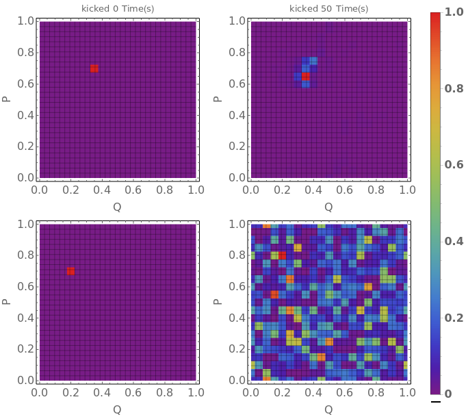
Figure 1: Two distinct dynamical evolutions of quantum kicked rotor with kicking strength $K=4.7$ and resolution $m=20$, i.e., effective Planck constant $\hbar_{\text{eff}}=2\pi/m^{2}\approx 0.016$. These two dynamical evolutions are generated by the same Hamiltonian but with different initial conditions(different Wannier basis states). See V. A for details

In this work we show that one can distinguish the two different types of quantum motions shown in Fig.1 by introducing a physical distance between quantum states based on the Wasserstein distance. Due to the use of the distance defined between basis vectors, our quantum distance is capable of quantifying the physical difference between quantum states. In particular, (1) it can reduce to the distance between classical states at the semiclassical limit; (2) it is not conserved during the quantum dynamical evolution; (3) it can be small or large between a pair of mutually orthogonal quantum states. This is qualitatively different from existing distances defined between quantum states, for example, Fubini-Study distanceKobayashi and Nomizu (1996). As a result, two quantum states, which are orthogonal to each other and initially close in the physical distance, can dynamically diverge from each other in the physical distance despite that the inner product stays at zero (see more detailed discussion at the beginning of Section IV). This physical distance allows us to define two parameters, quantum Lyapunov exponent and quantum chaos measure, to characterize quantum motion. Specially, the quantum chaos measure can be used to construct the quantum analogue of the classical Poicaré section, where we can map out the regions, where the quantum motion is regular (e.g., see Fig.5), and the regions, where the quantum motion is chaotic and depends sensitively on the initial condition (e.g., see Fig.5). This quantum Poicaré section reduces to its classical counterpart at the semiclassical limit.

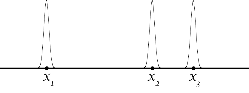
Figure 2: Three well localized wave packets at positions $x_{1}$, $x_{2}$ and $x_{3}$, respectively. There is no overlap between these wave packets. Physically, the two wave packets on the right are closer to each other.

We will introduce our definition of quantum physical distance in Sec. II. The soundness and usefulness of our distance is then illustrated with examples in Sec. III. In Sec. IV, with quantum physical distance, we define two parameters, quantum Lyapunov exponent and quantum chaos measure. The former characterizes the short-time dynamical behavior of a quantum state while the latter the long-time dynamical behavior of a quantum state. These concepts are numerically illustrated with three different quantum systems in Sec. V, which include the kicked rotor as the system which has a clear classical counterpart, a three-site Bose-Hubbard model whose classical counterpart is a mean field theory, and the spin-chain which does not have an obvious classical counterpart. Finally we discuss and conclude.

II Physical Distance Between Quantum States

Our physical distance between quantum states is based on the Wasserstein distance, which is a distance function defined between probability distributions on a metric space. In computer science it is known as the earth mover’s distance and has been widely used in many fieldsRubner et al. (2000); Orlova et al. (2016). To define a Wasserstein distance, we need both a metric space and a distribution function. To have them, for a quantum system, we choose a complete set of orthonormal basis $\mathcal{B}=\{\ket{\xi_{1}},\cdots,\ket{\xi_{n}}\}$ and define a distance between the bases $d(\xi_{i},\xi_{j})$. This gives us a metric space. When a given quantum state $\ket{\psi}$ is expanded in terms of this basis, we have a probability distribution on the set $\mathcal{B}$

$$p_{i}(\psi)=|\bra{\xi_{i}}\psi\rangle|^{2}\,,~{}~{}~{}~{}\ i=1,\cdots,n\,.$$ (1)

Our physical distance between two quantum states $\ket{\psi_{1}},\ket{\psi_{2}}$ is the Wasserstein-$\lambda$ distance between distributions $p_{i}(\psi_{1})$ and $p_{j}(\psi_{2})$

$$D_{\lambda}(\psi_{1},\psi_{2})=\Big{[}\inf_{P}\sum_{i,j}P_{ij}d^{\lambda}(\xi_{i},\xi_{j})\Big{]}^{1/\lambda}$$ (2)

where $\lambda$ is a positive integer and $\inf_{P}$ means the minimum over all the distributions $P_{ij}\in[0,1]$ that satisfy

$$\sum_{i=1}^{n}P_{ij}=p_{j}(\psi_{2})\ ;~{}~{}~{}~{}\sum_{j=1}^{n}P_{ij}=p_{i}(\psi_{1})\,.$$ (3)

It is clear that the above definition still works even when $n$ is infinite. For most of the cases studied in this work, we choose $\lambda=1$. This definition of physical distance can be generalized straightforwardly for mixed states. To do it, one only needs to specify the probability distribution as $p_{i}(\hat{\rho})=\text{Tr}(\ket{\xi_{i}}\bra{\xi_{i}}\hat{\rho})$ for a mixed state described by density matrix $\hat{\rho}$.

Two points warrant attention. (1) For a given quantum system, the choice of the orthonormal basis $\mathcal{B}$ is not unique. It depends on the physical issue that people want to address. For example, for a spin-lattice system, if we are interested in the magnetization along a given direction, then the spin up and down states in that direction are a natural choice and the distance $d$ for the metric can be chosen as the Hamming distance. (2) Our physical distance $D_{\lambda}$ is not a distance on the Hilbert space $\mathcal{H}$. There exists the states $\ket{\psi_{1}}\neq\ket{\psi_{2}}$ for whom $D_{\lambda}(\psi_{1},\psi_{2})=0$, for example, $\ket{\psi_{1}}=(\ket{\xi_{1}}+\ket{\xi_{2}})/\sqrt{2}$ and $\ket{\psi_{2}}=(\ket{\xi_{1}}-\ket{\xi_{2}})/\sqrt{2}$. Therefore, our distance is a function of states and basis, i.e., quantum states and the way to extract physical information from them. More thorough discussion will be given with examples in the following sections.

In Ref. Zyczkowski and Słomczyński (1998); Zyczkowski and Slomczynski (2001), a Monge distance was defined between quantum states with the Husimi function of a quantum state as the distribution. It shares two features with our distance: (1) mathematically, both are Wasserstein distance; (2) both reduce to the distance between classical states in the semiclassical limit $\hbar\rightarrow 0$. However, there is a crucial difference: the use of the orthonormal basis $\mathcal{B}$ and a metric defined over $\mathcal{B}$ in our definition. As a result, our physical distance is applicable for all quantum systems, including spin systems. If one is forced to view the Monge distance in this perspective, its choice of the orthonormal basis $\mathcal{B}$ is the points in the classical phase space and the metric is the usual distance between these points. This choice is certainly not natural as the Monge distance is defined for quantum states.

III Examples of Physical Distance

In this section, we use a few examples to illustrate the physical distance between quantum states. We will see that it can indeed capture quantitatively the physical difference between quantum states and is consistent with our physical intuition. There are various distances between quantum states based on the inner product of quantum states; for the sake of convenience, we compare our physical distance to one of them, Fubini-Study distance Kobayashi and Nomizu (1996).

The first example is a one-dimensional spinless particle and we are interested in its position. In this case, the basis $\mathcal{B}$ consists of infinite number of vectors $\ket{x}$, which are eigen-functions of position operator $\hat{x}$. We define the distance $d$ between two basis vectors $\ket{x}$ and $\ket{x^{\prime}}$ as $d(x,x^{\prime})=|x-x^{\prime}|$. Consider two different quantum states, $\ket{x_{1}}$ and $\ket{x_{2}}$. Then according to our definition, the physical distance between them is $D_{2}(x_{1},x_{2})=|x_{1}-x_{2}|$. In contrast, the Fubini-Study distance between $\ket{x_{1}}$ and $\ket{x_{2}}$ is one as long as $x_{1}\neq x_{2}$. Let us consider a Gaussian wave packet,

$$\braket{x}{\psi_{x_{0},p_{0};\sigma}}=\frac{1}{(2\pi\sigma^{2})^{\frac{1}{4}}}\exp\Big{[}-\frac{(x-x_{0})^{2}}{4\sigma^{2}}+i\frac{xp_{0}}{\hbar}\Big{]}\,.$$ (4)

One can find that the physical distance between two different Gaussian states is Olkin and Pukelsheim (1982)

$$D_{2}(\psi_{x_{1},p_{1};\sigma_{1}},\psi_{x_{2},p_{2};\sigma_{2}})=\sqrt{(x_{1}-x_{2})^{2}+(\sigma_{1}-\sigma_{2})^{2}}\,.$$ (5)

If the two Gaussian wave packets have the same width $\sigma_{1}=\sigma_{2}$, we simply have $D_{2}=|x_{1}-x_{2}|$, which is just what our physical intuition expects. In contrast, the Fubini-Study distance between these two Gaussian packets is close to one as long as $|x_{1}-x_{2}|\gg\sigma_{1,2}$. It is interesting to note that $D_{2}$ is independent of the momentum. This is reasonable as we are currently interested in the particle’s position. If one is interested in the particle’s momentum, one can similarly define $d(p,p^{\prime})=|p-p^{\prime}|$ and then find the physical distance in momentum between two Gaussian packets as

$$\widetilde{D}_{2}(\psi_{x_{1},p_{1};\sigma_{1}},\psi_{x_{2},p_{2};\sigma_{2}})=\sqrt{(p_{1}-p_{2})^{2}+(\tilde{\sigma}_{1}-\tilde{\sigma}_{2})^{2}}\,,$$ (6)

where $\tilde{\sigma}_{1,2}$ are the widths of the wave packets in the momentum space.

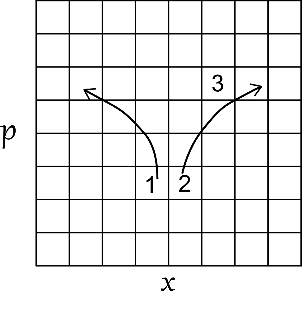
Figure 3: Quantum phase space of a one dimensional particle. $p$ and $x$ are its momentum and position, respectively. Each square represents a Planck cell. Three different Planck cells are marked by 1, 2, and 3.

The above simple example shows that the physical distance depends on what physics we want to explore. Mathematically, this is achieved by choosing an appropriate set of orthonormal basis $\mathcal{B}$. If we want to explore physics that is related explicitly to both position and momentum, we can choose $\mathcal{B}$ to be a set of Wannier basis. As shown in Fig.3, the classical phase space is divided into Planck cells and each Planck cell is assigned a Wanner function $\ket{w_{j}}$ von Neumann (1929, 2010); Han and Wu (2015); Fang et al. (2018). These orthonormal Wanner functions $\ket{w_{j_{x}j_{p}}}$ form the basis $\mathcal{B}$. We define

$$d(w_{j_{1}},w_{j_{2}})=\sqrt{(x_{j_{1}}-x_{j_{2}})^{2}+(p_{j_{1}}-p_{j_{2}})^{2}}\,,$$ (7)

where $x_{j}$’s and $p_{j}$’s are the coordinates of the Planck cells $\ket{w_{j}}$’s. Let us consider two Gaussian packets of the same width $\ket{\varphi_{1}}$ and $\ket{\varphi_{2}}$ in the quantum phase space, $\ket{\varphi_{1}}$ is centered at $\ket{w_{1}}$ and $\ket{\varphi_{2}}$ centered at $\ket{w_{2}}$. When the widths of two packets are much larger than a Planck cell and much smaller than the distance $d(w_{j_{1}},w_{j_{2}})$, we should have

$$\widetilde{D}_{1}(\phi_{1},\phi_{2})\approx\sqrt{(x_{1}-x_{2})^{2}+(p_{1}-p_{2})^{2}}\,,$$ (8)

where the approximation is due to that the Gaussian packets are discretized in the quantum phase space. This physical distance is reduced to the distance in the classical phase space when $\hbar\rightarrow 0$. The Fubini-Study distanceKobayashi and Nomizu (1996) does not have this kind of semi-classical limit.

We turn to many-body quantum states, and choose Fock states as the basis $\mathcal{B}$. A quantum state $\ket{n_{j}}=\ket{n_{1},n_{2},\cdots,n_{k}}$ means that there are $n_{j}$ particles in the single particle mode $\ket{e_{j}}$. The vacuum state is specially denoted as $\ket{e_{0}}=\ket{0,0,\cdots,0}$. We define a metric for the single-particle modes and the vacuum mode as $d(e_{i},e_{j})=d_{ij}=d_{ji}$ and $d(e_{i},e_{0})=d_{i0}=d_{0i}$. This allows us to define the distance between two Fock states $\ket{n_{j}}$ and $\ket{m_{j}}$

$$d(\ket{n_{j}},\ket{m_{j}})=\text{min}_{\Delta_{ij}}\sum_{i,j}d_{ij}\Delta_{ij}$$ (9)

where $n_{i}=\sum_{j}\Delta_{ij}$, $m_{j}=\sum_{i}\Delta_{ij}$, and $\Delta_{ij}\geq 0$. If the total number of particles in these two Fock states are different, we let $m_{0}=\max(\sum_{i}n_{i},\sum_{i}m_{i})-\sum_{i}m_{i}$ or $n_{0}=\max(\sum_{i}n_{i},\sum_{i}m_{i})-\sum_{i}n_{i}$ be the occupation number for the vacuum state $\ket{e_{0}}$. As a result, our definition is legal for states of different particle numbers. Note that the distance $d_{ij}$ can be defined differently for different systems and different physics that one is interested. Our definition has at least two advantages. First, it shares the same spirit with our physical distance, it is a Wasserstein-like metric for particle number distributions. Second, there is no exponential scaling between distance and particle number, which exists in the Fubini-Study distance.

We use a special case to illustrate the second point. Consider a system of $N$ identical Bosons and its two quantum states. In one state $\ket{\Psi_{1}}$, all the Bosons are in the mode $\ket{e_{1}}$; in the other state $\ket{\Psi_{2}}$, all the Bosons are in the state $\alpha\ket{e_{1}}+\beta\ket{e_{2}}$. It can be shown that $D_{1}(\Psi_{1},\Psi_{2})\propto N$. In contrast, the Fubini-Study distance is about $1-|\alpha|^{2N}$, which can be regarded as one when $N$ is large even when $\alpha\sim 1$, reflecting the fact that the two many-body states $\ket{\Psi_{1}}$ and $\ket{\Psi_{2}}$ are almost orthogonal to each other when $N$ is large no matter how close the single particle states $\ket{e_{1}}$ and $\alpha\ket{e_{1}}+\beta\ket{e_{2}}$ are to each other. So, our physical distance is more consistent with our intuition.

IV Quantum Dynamics and Physical distance

As quantum dynamics is linear, it is often said that there is no true chaos, in the sense of the chaos seen in nonlinear classical dynamics Berry (1988); Weinberg (Jan. 2017). The argument is as follows. Suppose that we have two quantum states $\ket{\psi_{1}}$ and $\ket{\psi_{2}}$. As quantum dynamics is linear, the inner product $\braket{\psi_{1}}{\psi_{2}}$ does not change with time. As a result, if these two states $\ket{\psi_{1}}$ and $\ket{\psi_{2}}$ are very close to each other, that is, $\braket{\psi_{1}}{\psi_{2}}\sim 1$, they will always be close to each other. This implies no true chaos. However, as shown in Fig.1, chaotic motion is clearly possible in quantum dynamics. Other examples of chaotic quantum motion can be found in Ref. Han and Wu (2016). This contradiction is due to the use of the inner product to measure the difference between quantum states. As already discussed, the inner product is incapable of telling us how close or far two quantum states are when they are orthogonal to each other.

Let us consider the case in Fig. 3. We use $\ket{w_{1}}$ and $\ket{w_{2}}$ to denote the two quantum states represented by the two Planck cells marked with 1 and 2. We let $\ket{w_{1}}$ and $\ket{w_{2}}$ to evolve, respectively, according to a given Schrödinger equation. As a result, at time $t$, $\ket{w_{1}}$ becomes $\ket{\phi_{1}(t)}$ and $\ket{w_{2}}$ evolves into $\ket{\phi_{2}(t)}$. The Fubini-Study distance between these two states does not change with time as $\braket{\phi_{1}}{\phi_{2}}=\braket{w_{1}}{w_{2}}=0$. However, it is very different story for physical distance. According to our discussion, the physical distance between $\ket{w_{1}}$ and $\ket{w_{2}}$ is small. When the dynamical evolution starts, the physical distance can grow. The linearity of quantum dynamics does not guarantee that the physical distance between $\ket{\phi_{1}(t)}$ and $\ket{\phi_{2}(t)}$ be small. The situation shown in Fig. 3 can happen: the physical distance grows with time in quantum dynamics while keeping $\braket{\phi_{1}}{\phi_{2}}$ at zero. As we will show with our numerical calculation in the next section, this is indeed what happens in quantum chaotic systems.

So, there is true chaos in quantum dynamics and it can be understood in terms of physical distance. In the following, using the concept of physical distance, we define two parameters to characterize the diverging and irregular quantum dynamics.

IV.1 Quantum Lyapunov Exponent

Lyapunov exponent is one of the most important concepts in classical dynamics and it characterizes the rate of separation of infinitesimally close initial trajectories. Quantitatively, in a chaotic classical dynamics, the distance (usually $L_{2}$ distance) between two points that are initially very close grows with time $t$ as

$$\|\delta\bm{Z}(t)\|\approx e^{\gamma t}\|\delta\bm{Z}(t=0)\|$$ (10)

where $\bm{Z}=(q,p)$ is the state in phase space. The parameter $\gamma$ is the Lyapunov exponent. With the physical distance between two quantum states, the (maximum) Lyapunov exponent in quantum mechanics can be similarly defined asMan’ko and Vilela Mendes (2000); Zyczkowski et al. (1993)

$$\gamma_{Q}=\lim_{t\rightarrow\infty}\lim_{\psi^{\prime}\rightarrow\psi}\frac{1}{t}\log\frac{D(\psi(t),\psi^{\prime}(t))}{D(\psi(0),\psi^{\prime}(0))}$$ (11)

This is very similar to the definition of Lyapunov component in classical mechanics, which can be obtained by replacing the physical distance between states $D(\cdot,\cdot)$ with the distance in classical phase space. The symbol $\psi^{\prime}\rightarrow\psi$ means $\psi,\psi^{\prime}$ are close but different in the sense of physical distance.

For quantum systems where quantum phase spaces similar to Fig.3 can be constructed, we can always use physical distance similar to the one in Eq.(6). In the semi-classical limit, $\hbar\rightarrow 0$, the areas or volumes of the Planck cells approach zero and the quantum dynamics becomes classical. In this limit, we should have

$$\lim_{\hbar\rightarrow 0}\gamma_{Q}=\gamma_{C}\,.$$ (12)

Note that this relation holds only when the Lyapunov time (the inverse of Lyapunov exponent) is smaller than the Ehrenfest time Han and Wu (2016); Zhao and Wu (2019). So the limit $t\rightarrow\infty$ is not a strict mathematical term and should be understood as a sufficiently long time before the wave packets become too widely spread.

IV.2 Quantum Chaos Measure

Intuitively, chaos means disorder and irregularity in dynamics. In classical dynamics, this is indicated by the scattered points in Poincaré sections (see, e.g., Fig.5(a)), which are usually referred to as chaotic sea. How chaotic a classical dynamics is reflected by how much the chaotic seas occupy in the phase space. In the chaotic sea, there are regular motions, which are usually referred to as integrable island. When there is only “chaotic sea” in the Poincaré sections, the system becomes fully chaotic In this case, we have ergodicity and/or mixing and the long-time average becomes identical to the microcanonical ensemble average Zhang et al. (2016).

With physical distance, we can also compare the long-time average and the microcanonical ensemble average for quantum dynamics. In standard textbooks Huang (1987), the microcanonical ensemble is regarded as a maximally mixed state and can be described by the density matrix $\hat{\mathbb{I}}/{\rm Dim}$. $\hat{\mathbb{I}}$ is the identity matrix and Dim is the dimension of the Hilbert space. This is usually a postulate in standard textbooks Huang (1987). But it has been fully justified by many studies von Neumann (1929, 2010); Reimann (2008); Han and Wu (2015); Zhang et al. (2016). We use the physical distance between the long-time-average of the density matrix and the density matrix $\hat{\mathbb{I}}/{\rm Dim}$ to quantitatively measure the severity of quantum chaos. Mathematically, this difference is given by

$$\Upsilon=D\Big{(}\frac{1}{\text{Dim}},\lim_{T\rightarrow\infty}\frac{1}{T}\int_{0}^{T}\hat{\rho}(t)\text{d}t\Big{)}$$ (13)

We call it quantum chaos measure. The measure $\Upsilon$ depends on the initial quantum states. For some initial quantum states, $\Upsilon$ is small and it means that the long-time-average density matrix is sufficiently close to the maximally mixed state. These quantum states belong to chaotic sea. For some initial states, $\Upsilon$ is large and these states belong to integrable islands. In the next section, our numerical results will show that we can use chaos measure to construct quantum Poincaré sections, which resemble classical Poincaré sections.

One can use other tools to quantify the degree of disorder in quantum dynamics, for example, quantum entropy of the form $-\sum_{i}p_{i}\log p_{i}$ Jiang et al. (2017); Hu et al. (2019). The core advantage of our chaos measure is its dependence on the metric structure of basis $\mathcal{B}$, i.e., the information of base space. For example (see Appendix B for detail), consider the following two probability distributions on set $\{0,1,2,\cdots,9\}$

$$p_{A}(x)=\begin{cases}1/5&x<5\\ 0&x\geq 5\end{cases}$$ (14)

and

$$p_{B}(x)=\begin{cases}1/5&x\text{ is even}\\ 0&\text{otherwise}\end{cases}$$ (15)

The entropies of $p_{A}$ and $p_{B}$ are the same, but $p_{B}$ appears much closer to the uniform distribution. This can be reflected by our chaos measure as we have $\Upsilon_{A}=5/2\ ;\ \Upsilon_{B}=1/2$ with the metric $d(x,y)=|x-y|$ on the base space. This difference means our measure $\Upsilon$ can reveal finer property better than any other concepts that ignore the information of the base space. In Ref.Yin et al. (2019), the length of a Planck cell was introduced to measure disorder in quantum dynamics; however, this concept is limited and can not be applied to spin systems.

V Numerical Results

In this section, we will numerically study three different systems to illustrate the concept of physical distance. These three systems are quantum kicked rotor, three-site Bose-Hubbard model, and XXZ spin chain. The quantum kicked rotor has a natural classical counterpart. For the three-site Bose-Hubbard model, its classical counterpart is the mean-field theory and its effective Planck constant is the inverse of the particle number $1/N$. In contrast, the XXZ spin chain has no obvious classical counterpart.

V.1 Kicked Rotor

Kicked rotor is one of the systems which have been well studied both as a quantum and classical system. The Hamiltonian of a kicked rotor on a ring has the following dimensionless form Jiang et al. (2017); Yin et al. (2019)

$$H=\frac{1}{2}p^{2}+K\cos q\sum_{n=-\infty}^{+\infty}\delta(t-n)$$ (16)

Its classical dynamics is equivalent to the following map

$$p_{n+1} =p_{n}+K\sin q_{n}\mod 2\pi$$ (17)

$$q_{n+1} =q_{n}+p_{n+1}\mod 2\pi$$

where we have used the fact that the momentum $p$ and $p+2n\pi$ are equivalent. $(q_{n},p_{n})$ is the position and momentum of the kicked rotor before the $n$-th kick. The kicking strength $K$ is the only control parameter; when it is bigger than $K_{c}=0.971635$ the classical dynamics becomes chaoticChirikov and Shepelyansky (2008).

The quantum dynamics has one more parameter, the effective Planck constant $\hbar_{\rm eff}$ Jiang et al. (2017); Yin et al. (2019). For simplicity, we choose $\hbar_{\rm eff}=2\pi/m^{2}$ with $m$ being an positive integer. In this case, we can divide the $2\pi\times 2\pi$ classical phase space into $m\times m$ Planck cells (similar to Fig. 3) and assign a Wannier function $\ket{X,P}$ to each Planck cell Jiang et al. (2017); Yin et al. (2019). $X,P$ are the coordinates of a Planck cell. These Wannier functions $\{\ket{X,P}\}$ form a complete set of orthonormal basis. We choose them as our choice of $\mathcal{B}$ and define the distance between two basis vectors as $d(X,P;X^{\prime},P^{\prime})=\sqrt{(X^{\prime}-X\mod 2\pi)^{2}+(P^{\prime}-P\mod 2\pi)^{2}}$.

In our numerical calculation, we choose the initial quantum states localized at $(4.7,3)$ and $(4.7+2\pi/m,3+2\pi/m)$. The dynamics near these two points becomes chaotic as $K$ increases as shown in Fig.5(a,c). The initial quantum states are the maximally localized Gaussian wave packets of the following form

$$\langle x\ket{\psi(x_{0},p_{0})}=\frac{1}{(2\pi\hbar_{\text{eff}})^{1/4}}\exp\Big{[}-\frac{(x-x_{0})^{2}}{2\hbar_{\rm eff}}+\frac{\text{i}xp_{0}}{\hbar_{\rm eff}}\Big{]}$$ (18)

As the two states evolve with time, we compute numerically the physical distance between them and see how they change with time. For comparison, we have also computed two other distances. One is the distance between the expectation values of $\hat{q},\hat{p}$ for these two different quantum states. For convenience, we call it expectation distance. The other is the distance between two corresponding classical trajectories starting at $(4.7,3)$ and $(4.7+2\pi/m,3+2\pi/m)$. The results are plotted in Fig.4.

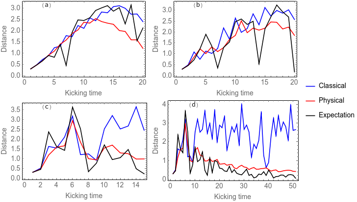
Figure 4: The time evolution of three types of distances for the kicked rotor at different kick strengths $K$. Blue lines are the distances between the points on classical trajectories, red lines are physical distance between wave packets in the quantum phase space, and black lines are the distance between the expectation values of operators $\hat{q},\hat{p}$. (a) $K=0.3$, $m=30$; (b) $K=0.9$, $m=30$; (c) $K=1.5$, $m=30$. (d) has the same parameters $K=1.5$, $m=30$ but with a longer time evolution.

It is clear from Fig.4 that the physical distance agrees very well with the classical distance for the first several kicks. In contrast, during these kicks, the expectation distance can deviate largely from the classical distance. As the evolution goes on, both physical distance and expectation distance deviate far from the classical distance as expected because the wave packets get distorted. When $m$ is sufficiently large or, equivalently, $\hbar_{\rm eff}$ is small enough, the Ehrenfest time would be longer than the Lyapunov time. In these cases, we should see that the physical distance agree with the classical distance for a much longer time; as a result, we would be able to estimate numerically the quantum Lyapunov exponent. Unfortunately, due to our limited computation power, we can not compute for very large $m$.

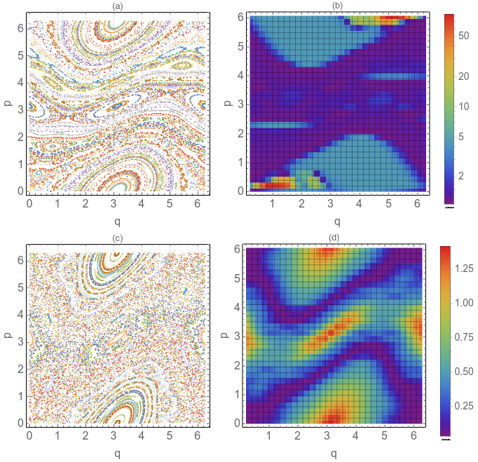
Figure 5: (a)(c) Classical Poincaré sections and (b)(d) quantum chaos measures in the quantum phase space. The chaos measure for a Planck cell is computed by the evolution of a quantum state which is initially localized at the Planck cell. The figures are plotted by scanning the entire quantum phase space. Note that plotted in (b) is colored with logarithm scaling and the original values range is $[1.07,82.3]$. In (d), the values of chaos measure range in $[0.03,1.41]$.

We have also computed quantum chaos measure for the kicked rotor. We use the maximally localized Gaussian wave packets as the initial states, scan the entire quantum phase space, and compute the measure for each Planck cell. The results are plotted in Figs. 5(b,d) and compared to the classical Poincaré sections in Figs. 5(a,c). The resemblance between them is unmistakeable. Note that the chaos measure is the distance between long-time averaged density matrix and the maximally mixed state. In Figs. 5(b), the values of our measure are very large for many Planck cells. This means that the wave packets starting at these Planck cells do not spread out much and stay near the original Planck cells (e.g. see the upper panels in Fig. 1). When the kicking strength $K$ is large, the values of the measure become much smaller, indicating that the quantum dynamics become more chaotic and the wave packets began to spread out to the large portions of the phase space (e.g. see the lower panels in Fig. 1).

V.2 Three-site Bose-Hubbard Model

We consider a different system, a three-site Bose-Hubbard model described by the following Hamiltonian Han and Wu (2016)

$$\hat{H}=-\frac{c_{0}}{2}\sum_{\begin{subarray}{c}1\leq i,j\leq 3\\ i\neq j\end{subarray}}\hat{a}_{i}^{\dagger}\hat{a}_{j}+\frac{c}{2N}\sum_{j=1}^{3}\hat{a}_{j}^{\dagger}\hat{a}_{j}^{\dagger}\hat{a}_{j}\hat{a}_{j}\,,$$ (19)

where $\hat{a}_{j}^{\dagger}$ and $\hat{a}_{j}$ are the Bosonic creation and annihilation operators for the mode $j$. $c$ is the scaled interaction strength and $N$ is the number of Bosons in the system. This system has a mean-field limit at $N\rightarrow\infty$, whose Hamiltonian is

$$H_{\text{mf}}=-\frac{c_{0}}{2}\sum_{\begin{subarray}{c}1\leq i,j\leq 3\\ i\neq j\end{subarray}}a_{i}^{*}a_{j}+\frac{c}{2}\sum_{j=1}^{3}|a_{j}|^{4}\,,$$ (20)

where $|a_{1}|^{2}+|a_{2}|^{2}+|a_{3}|^{2}=1$. In this Bose-Hubbard model, the quantumness is controlled by the particle number $N$ and the mean field Hamiltonian is its “classical counterpart”. As we will show, the physical distance is still applicable in this type of systems.

Since in the mean-field model each mode $a_{j}$ has a definite amplitude and phase, we choose a basis $\mathcal{B}$ for the quantum model where each basis vector contains information for both amplitude (or particle number) and phase. For convenience, we take the total particle number $N=L^{2}-1$, where $L$ is an integer. The basis vector in $\mathcal{B}$ is denoted as $\ket{\ell_{1},\vartheta_{1};\ell_{2},\vartheta_{2}}$; its expectations for particles numbers are $\ell_{1,2}L+(L-1)/2$ and for phases $2\pi\vartheta_{1,2}/L$. The details of this orthonormal basis $\{\ket{\ell_{1},\vartheta_{1};\ell_{2},\vartheta_{2}}\}$ with $0\leq\ell_{1,2},\vartheta_{1,2}\leq L-1$ can be found in Appendix A. This effectively creates a 4-dimensional quantum phase space with $L\times L\times L\times L$ Planck cells. Therefore, a natural choice for the basis metric is

$$d(\{\ell,\vartheta\},\{\ell^{\prime},\vartheta^{\prime}\})=\frac{1}{L}\sqrt{\sum_{i=1}^{2}\big{(}\Delta\ell_{i}^{2}+\Delta\vartheta_{i}^{2}\big{)}}$$ (21)

where $\Delta\ell_{i}=|\ell_{i}-\ell^{\prime}_{i}|$ and $\Delta\vartheta_{i}=\min\{|\vartheta_{i}-\vartheta^{\prime}_{i}|,L-|\vartheta_{i}-\vartheta^{\prime}_{i}|\}$($\vartheta_{i}$ is periodic). We can compute the physical distance between two quantum states or two classical points according to this metric just like what we did for the kicked rotor.

The classical motion of the system is nonintegrable for generic $c$. This is evident in the Poincaré section for $c/c_{0}=2$, $E=0.8c_{0}$, $n_{2}=0.2475$, $\dot{n}_{2}>0$ shown in Fig.7a, where we see both regular and chaotic motions. Note that $n_{1,2}=|a_{1,2}|^{2}$ and $\theta_{1,2}={\rm arg}a_{1,2}-{\rm arg}a_{3}$. We choose the quantum initial state to be a coherent state $|\Psi\rangle=\frac{1}{\sqrt{N!}}\left(\sum_{i=1}^{3}a_{i}\hat{a_{i}}^{\dagger}\right)^{N}|0\rangle$; its shape in our quantum phase space will be close to a Gaussian packet centered at the classical point $(a_{1},a_{2},a_{3})^{\mathrm{T}}$ with a width of order $\sqrt{1/N}\sim 1/L$ Han and Wu (2016).

We first choose a pair of initial conditions, $(n_{1},\theta_{1})=(0.220,0.8\pi)$ and $(n_{1},\theta_{1})=(0.221,0.8\pi)$, which are located in the integrable island of the Poincaré section in Fig.7a. The results are presented in Fig.6a. It can be seen that, when the dynamics is regular, the quantum physical distance coincides with the classical distance very well in a relatively long period of time. When the quantum resolution $L$ is increased from 6 to 9, the quantum physical distances have an obvious inclination to converge to the classical distance. This is quite surprising because the difference between two initial conditons is only of order $10^{-3}$ while for the highest quantum resolution $L=9$ in our simulation the size of the Planck cell is of order $10^{-1}$. So, we expect that our physical distance match classical distance well even when the size of the Planck cell is significantly smaller than the classical distance between two initial conditions.

We choose a different pair of initial conditions, $(n_{1},\theta_{1})=(0.420,0.8\pi)$ and $(n_{1},\theta_{1})=(0.421,0.8\pi)$, which are located in the chaotic sea of Fig.7a. The numerical results are shown in Fig. 6b. In this chaotic case, the total time that the quantum physical distances and the classical distance coincide is much shorter. This can be explained with the Ehrenfest time, the time scale when the quantum-classical dynamics breakdown. For the chaotic dynamics, the Ehrenfest time is short and proportional to $\ln N$Han and Wu (2016), while for the integrable dynamics this timescale is much longer and proportional to $\sqrt{N}$ Zhao and Wu (2019). So, for this chaotic dynamics, to see numerically exponential divergence of the quantum physical distance, we have to have $N$ (or $L$) exponentially large. Unfortunately, for both integrable and chaotic cases, large $N$ is beyond our numerical capacity.

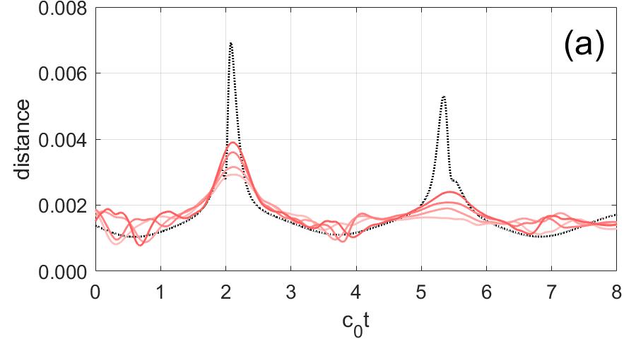
(a)

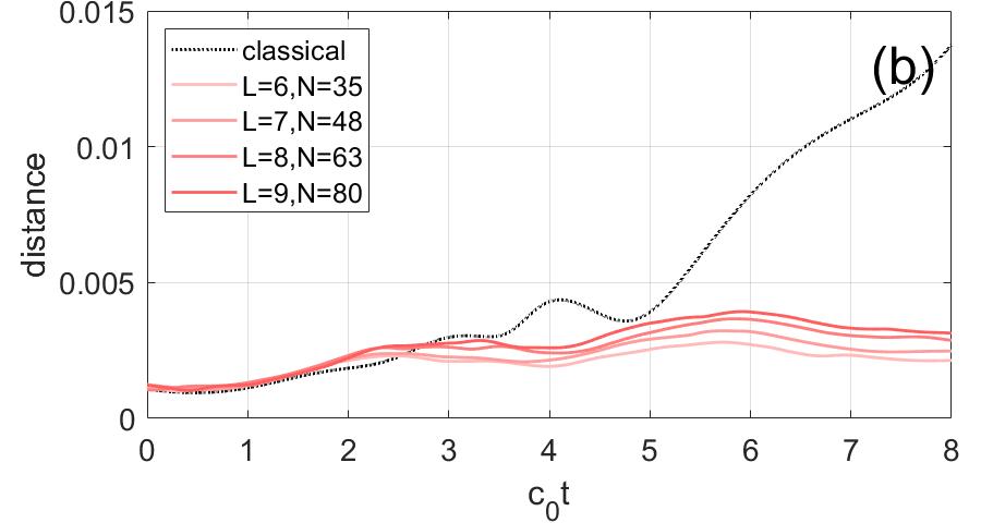
(b)

Figure 6: Physical distances between two pairs of perturbed initial conditions: (a) regular case, $(n_{1},\theta_{1})=(0.220,0.8\pi)$ and $(0.221,0.8\pi)$; (b) chaotic case, $(n_{1},\theta_{1})=(0.420,0.8\pi)$ and $(0.421,0.8\pi)$. Both are chosen from the Poincaré section in Fig.7a. The regular classical distance is well recovered by quantum distances for time up to $c_{0}t=8$, and the sharp peaks in the classical distance curve is also prominent in quantum curves. As the quantum phase space resolution $L$ is increased, the peaks become closer and closer to the classical one. In the chaotic case, although the quantum distance start deviating from the classical distance at an earlier stage due to a fast Ehrenfest breakdown, its smoothness stands in sharp contrast to the rich structure in regular classical distance curves as well as regular quantum distance curves, demonstrating the stark difference between regular motion and chaotic motion.

(a)

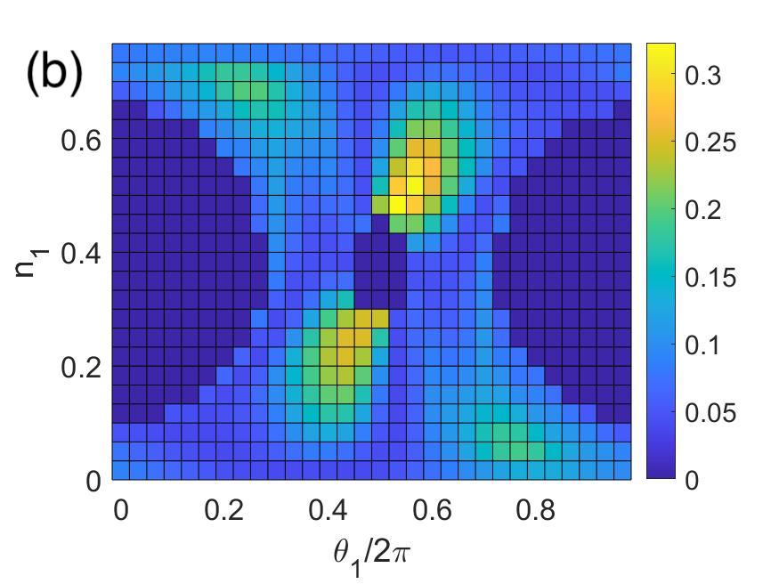
(b)

Figure 7: (a) Classical Poincaré section of the mean-field model (see Eq.(20)) at $c/c_{0}=2$, $E=0.8c_{0}$, $n_{2}=0.2475$, $\dot{n}_{2}>0$. (b) The corresponding quantum chaos measure with $L=10$ (see main text for computation details). Note that the side length of little squares in (b) is equal to 1/(3L), the sampling step length, instead of the inverse resolution $1/L$. It is clear that the yellow and green areas, where the quantum chaos measure is large, coincide with the classical regular islands while the blue areas, the quantum chaos measure is small, correspond to the chaotic sea.

We also computed quantum chaos measure for this Bose-Hubbard system, corresponding to the classical Poincaré section in Fig.7a with $c/c_{0}=2$. We divide the phase space with the quantum resolution $L=10$, that is, the total particle number being $N=99$. Our initial quantum states are coherent states $|\Psi_{c}(t=0)\rangle$, which are localized wavepackets occupying $O(1)$ Planck cells. We calculate their long-time average density matrix $\rho_{\infty}=\lim_{T\to\infty}\frac{1}{T}\int_{0}^{T}\mathrm{d}t|\Psi_{c}(t)\rangle\langle\Psi_{c}(t)|$, and project them onto the quantum phase space and obtain the distribution $P_{c}(\ell_{i},\vartheta_{i})=\mathrm{Tr}\{\rho_{\infty}|\ell_{i},\vartheta_{i}\rangle\langle\ell_{i},\vartheta_{i}|\}$. The classical (or mean-field) dynamics is limited to a constant energy surface in the phase space. In contrast, the quantum dynamics is limited to an energy shell with certain thickness. To effectively reduce the computation burden, we only pick out Planck cells located within the Gaussian-broadening energy shell. To be specific, we Gaussian fit the smoothened envelope of the energy spectrums of these selected coherent states, with the fitting goodness $R^{2}=0.994$, and select out the phase cells with energy expectation values within $\pm 3\sigma$ of the Gaussian. This method is able to capture $70\%\pm 7\%$ of the original coherent packets. We then set the energy shell with this Gaussian envelope to be the ergodic reference $\rho_{\rm erg}$ of the system following Heller (1987), in place of the classical microcanonical ensemble, and project it onto the space $P_{\rm erg}(\ell_{i},\vartheta_{i})=\mathrm{Tr}\{\rho_{\rm erg}|\ell_{i},\vartheta_{i}\rangle\langle\ell_{i},\vartheta_{i}|\}$. Then we calculate the physical distance between $P_{\rm erg}(\ell_{i},\vartheta_{i})$ and each $P_{c}(\ell_{i},\vartheta_{i})$ and obtain the chaos measure. The results are plotted in Fig.7b. We see that the classical Poincaré section in Fig.7a is very well recovered. The regular islands are distinguished by the coherent initial states that have a large physical distance from the ergodic envelope, while the chaotic sea is filled with initial states that are very close in physical distance to the ergodic envelope. Quite surprisingly, even the two small regular islands with size of only one single quantum phase cell are clearly seen. Therefore, we expect our chaos measure proposed here is able to distinguish regular island structures with size no smaller than the order of one single Planck cell.

V.3 Spin Chain

We now study a system which does not have a clear classical counterpart. It is the spin-1/2 XXZ model with disorder described by the following Hamiltonian Gubin and F. Santos (2012)

$$\hat{H}=\sum_{i=0}^{N-1}h_{i}\hat{s}_{i}^{z}+\sum_{i=0}^{N-2}\Big{\{}J_{1}\big{(}\hat{s}_{i}^{x}\hat{s}_{i+1}^{x}+\hat{S}_{i}^{y}\hat{s}_{i+1}^{y}\big{)}+J_{2}\hat{s}_{i}^{z}\hat{s}_{i+1}^{z}\Big{\}}\,,$$ (22)

where $\hat{s}_{i}^{x,y,z}$ are spin operators at the $i$th site and $h_{i}=\epsilon\delta_{i,i^{*}}$ is the magnetic field at a given random site denoted by $i^{*}$. In our model, $S^{z}=\sum_{i=1}^{N}s^{z}_{i}$ is conserved and the Hilbert space can be divided into subspaces labelled by $S^{z}$. The spin system has different eigen-energy spacing statistics with different values of $\epsilon$ Gubin and F. Santos (2012). Two examples are shown in Fig. 8, which show that the case $\epsilon=0.01$ is largely integrable while the case $\epsilon=0.5$ is chaotic.

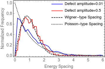
Figure 8: Eigen-energy spacing statistics for the XXZ spin chain that has $15$ spins in the sub-Hilbert space with $5$ spins up. The defection is on the site $i^{*}=2$ and the boundary condition is open with $J_{1}=1.0$, $J_{2}=0.5$. The red line is for $\epsilon=0.5$ and is close to the Wigner-Dyson distribution (dashed line) while the blue line is for $\epsilon=0.01$ and is close to Poison distribution(dotted line).

To compute the quantum chaos measure, we choose the set of common eigenstates of all $\hat{s}_{i}^{z}$ as the basis $\mathcal{B}$ and denote them as $0,1$ valued vectors $\{\ket{s_{1},s_{2},\cdots,s_{N}}\}_{s_{i}\in\{0,1\}}\}$. The distance between them is defined as the $L_{1}$ measure between the arrays of positions of $1$s. For example, the array for the positions of $1$s in the state $\ket{1,1,0,0,0}$ is $(0,1)$, and the array for $\ket{0,0,0,1,1}$ is $(3,4)$. So, the distance between them is

$$d(\ket{1,1,0,0,0},\ket{0,0,0,1,1})=|3-0|+|4-1|=6$$ (23)

Note that this metric is different from the Hamming distance, which is $4$ between the states $\ket{1,1,0,0,0}$ and $\ket{0,0,0,1,1}$. In fact, this metric is the same as our distance defined for the many-body states in Sec. III if we treat the states $\ket{s_{1},\cdots,s_{N}}$ as Fock states for Fermions with $s_{j}$ particle in the single particle mode $\ket{j}$ and define the distance between corresponding single particle states $\ket{j}$’s as $d(\ket{i},\ket{j})=|i-j|\ ;\ i,j=1,\cdots,N$. For example, the most efficient way to transport $(1,1,0,0,0)$ to $(0,0,0,1,1)$ is to move each $1$ in the first array to the position of corresponding $1$s one by one in the second array.

In our numerical computation, we choose $N=15$ and focus on the subspace with $5$ spins up. The initial localized states are chosen to be states that have consecutive $1$s in their boolean-valued arrays, such as $(1,1,1,1,1,0,\cdots,0)$ and $(0,1,1,1,1,1,\cdots)$. There are in total ten of them, which are numbered according to the position of the first $1$. The computed quantum chaos measure is shown in Fig.9. It is clear from the figure that the chaos measure is much smaller for the chaotic case $\epsilon=0.5$ than for the non-chaotic case $\epsilon=0.01$. This is in agreement with the eigen-energy spacing statistics shown in Fig. 8.

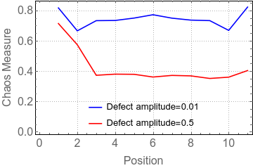
Figure 9: Quantum chaos measures for the $10$ initially localized states in the XXZ spin chain model. The green line is for $\epsilon=0.01$ and the red line for $\epsilon=0.5$. The left side of the red line is large is caused by the defection on the second site $i^{*}=2$. The overall decrease of the chaos measure from $\epsilon=0.01$ to $\epsilon=0.5$ shows the spin chain becomes more chaotic as the defection increases, which agrees the results of energy spacing statistics.

VI Discussion and Conclusion

In some cases the Wasserstein distance is not robust with respect to the distance matrix $d_{ij}$ defined for a pair of basis vector. For example, consider two distribution: $\delta(x)$ and $(1-\eta)\delta(x)+\eta\delta(x-d)$ on a one dimensional Euclidean space. The Wasserstein distance between them is nothing but $\eta d$. That means no matter how small $\eta$ is, one can find a sufficient large $d$ so that the Wasserstein distance diverges. That is what we meant by that the distance is not robust with respect to $d_{ij}$ . Fortunately, the distance matrix $d_{ij}$ in our numerical examples have upper bounds so that we do not need to worry about this.

Another challenge for our proposed physical distance is the complexity of computing the Wasserstein distance. In our numerical implement, we use python module named pyemd to compute the Wasserstein distance Pele and Werman (2008, 2009). Though the convex optimization problem for computing the distance is easy (it is a linear programing problem in discretized formOberman and Ruan (2015)), we are facing an exponentially high dimensional Hilbert space in quantum mechanics and our code can not handle larger systems. But the core of this challenge is the dimension of the Hilbert space, which should also be a challenge to any other definitions with the similar concept. In this sense, our definition has an equivalent complexity to others.

In conclusion, we have shown that there is genuine quantum chaos despite that quantum dynamics is linear. This is revealed with the physical distance that we proposed for two quantum states. This quantum distance is based on the Wasserstein distance between two probability distributions. We call it ”physical” because it faithfully measures the difference of physical properties. This physical distance can be very small for two orthogonal initial quantum states, and then diverge exponentially during the ensuing quantum chaotic motion. With physical distance, we have defined two parameters to characterize the quantum dynamics: quantum Lyapunov exponents for the short time dynamics and quantum chaos measure for the long time dynamics. The latter allows us to construct the quantum analogue of the classical Poincaré section, where regions for regular quantum motions and chaotic quantum motions are mapped out.

Appendix A Quantum phase space for the three-site Bose-Hubbard model

A.1 Construction of the quantum phase space

The total particle number $N$ is conserved in the three-site Bose-Hubbard Hamiltonian (Eq. 19). As a result, in the Fock states $|N_{1},N_{2},N_{3}\rangle$, there are only two free parameters $N_{1,2}$ and $N_{3}=N-N_{1}-N_{2}$. We consider a Hilbert space spanned by Fock states $|N_{1},N_{2}\rangle$ with $0\leq N_{1,2}\leq N$, which contains the Hilbert space of the three-site Bose-Hubbard system. We further take $N=L^{2}-1$. For this $L^{4}$-dimensional Hilbert space, we define a set of orthonormal basis

$$|\ell_{1},\vartheta_{1};\ell_{2},\vartheta_{2}\rangle=$$ (24)

$$\frac{1}{L}\sum_{N_{1}=0}^{L-1}\sum_{N_{2}=0}^{L-1}e^{i\frac{2\pi}{L}(N_{1}\vartheta_{1}+N_{2}\vartheta_{2})}|N_{1}+\ell_{1}L,N_{2}+\ell_{2}L\rangle\,,$$

where the four indices $\ell_{1,2},\vartheta_{1,2}=0,1,...,L-1$. As a result, the $L^{4}$-dimensional Hilbert space is arranged into a 4-dimensional phase space which is divided into $L\times L\times L\times L$ Planck cells. And each Planck cell is represented by $\ket{\ell_{1},\vartheta_{1};\ell_{2},\vartheta_{2}}$. For this 4-dimensional phase space, there are two pairs of conjugate observables, $\hat{N}_{1,2}$, the particle number operators , and $\hat{\theta}_{1,2}$, the relative phase operators. They can be defined as

$$\hat{N}_{i} = \sum_{N_{1}=0}^{N}\sum_{N_{2}=0}^{N}N_{i}|N_{1},N_{2}\rangle\langle N_{1},N_{2}|,$$ (25)

$$\hat{\theta}_{i} = \sum_{M_{1}=0}^{N}\sum_{M_{2}=0}^{N}\theta_{M_{i}}|\theta_{M_{1}},\theta_{M_{2}}\rangle\langle\theta_{M_{1}},\theta_{M_{2}}|,$$ (26)

where $|\theta_{M_{1}},\theta_{M_{2}}\rangle$ is the Fourier transformation of the Fock basis

$$|\theta_{M_{1}},\theta_{M_{2}}\rangle=\frac{1}{N+1}\sum_{N_{1}=0}^{N}\sum_{N_{2}=0}^{N}e^{i(N_{1}\theta_{M_{1}}+N_{2}\theta_{M_{2}})}|N_{1},N_{2}\rangle$$ (27)

with $\theta_{M_{i}}=\theta_{i}^{(0)}+2\pi M_{i}/(N+1)$ and $M_{i}=0,1,...,N$. In light of this, we can recast Eq.(24) into

$$|\ell_{1},\vartheta_{1};\ell_{2},\vartheta_{2}\rangle=$$ (28)

$$\frac{1}{L^{3}}\sum_{M_{1}=0}^{N}\sum_{M_{2}=0}^{N}\frac{1-e^{-iL(\theta_{M_{1}}-\frac{2\pi\vartheta_{1}}{L})}}{1-e^{-i(\theta_{M_{1}}-\frac{2\pi\vartheta_{1}}{L})}}\frac{1-e^{-iL(\theta_{M_{2}}-\frac{2\pi\vartheta_{2}}{L})}}{1-e^{-i(\theta_{M_{2}}-\frac{2\pi\vartheta_{2}}{L})}}$$

$$~{}~{}~{}~{}~{}~{}~{}~{}~{}~{}~{}~{}~{}\times e^{-iL(\ell_{1}\theta_{M_{1}}+\ell_{2}\theta_{M_{2}})}|\theta_{M_{i}},\theta_{M_{2}}\rangle$$

where each fraction takes its limit value if its denominator is 0.

We will show in the follow that each $|\ell_{1},\vartheta_{1};\ell_{2},\vartheta_{2}\rangle$ state represents a Planck cell in the phase space in the sense that their positions are fixed by the four parameters $\ell_{i},\vartheta_{i}$, and that their shapes are localized.

A.2 The positions of the Planck cells

We will analytically verify that for a given Planck cell $|\ell_{1},\vartheta_{1};\ell_{2},\vartheta_{2}\rangle$, $\ell_{i}$ is proportional to the expectation value of particle number at this cell and $\vartheta_{i}$ is proportional to the expectation value of the phase, up to some correction terms. The expectations are

$$\langle\hat{N}_{i}\rangle_{\ell_{i},\vartheta_{i}} = \ell_{i}L+\frac{L-1}{2},$$ (29)

$$\langle\hat{\theta}_{i}\rangle_{\ell_{i},\vartheta_{i}} = \frac{2\pi}{L}\vartheta_{i}+\frac{1}{L^{3}}\sum_{M_{i}=0}^{N}\left|\frac{\sin\frac{L\tilde{\theta}_{M_{i}}}{2}}{\sin\frac{\tilde{\theta}_{M_{i}}}{2}}\right|^{2}\tilde{\theta}_{M_{i}},$$ (30)

where $\langle\cdot\rangle_{\ell_{i},\vartheta_{i}}$ denotes the expectation value of the state $|\ell_{1},\vartheta_{1};\ell_{2},\vartheta_{2}\rangle$, and $\tilde{\theta}_{M_{i}}=\theta_{M_{i}}-\frac{2\pi}{L}\vartheta_{i}$. The normalization of Eq.(28) has been used in deriving Eq.(30).

We can further show that the correction terms can be regarded as constants independent of $\vartheta_{i}$. In Eq.(29), this is obvious. We only need to examine Eq.(30). We notice that in Eq.(30), with fixed $\theta^{(0)}_{i}$, altering $\vartheta_{i}\to\vartheta_{i}+1$ is equivalent to adding an additional term to $\theta_{M_{i}}\to\theta_{M_{i}}-2\pi/L$, and keeping $\vartheta_{i}$ unchanged,

$$\frac{1}{L^{3}}\sum_{M_{i}=0}^{N}\left|\frac{\sin\frac{L\tilde{\theta}_{M_{i}}}{2}}{\sin\frac{\tilde{\theta}_{M_{i}}}{2}}\right|^{2}\tilde{\theta}_{M_{i}}$$ (31)

$$\to\frac{1}{L^{3}}\sum_{M_{i}=0}^{N}\left|\frac{\sin\frac{L(\tilde{\theta}_{M_{i}}-2\pi/L)}{2}}{\sin\frac{\tilde{\theta}_{M_{i}}-2\pi/L}{2}}\right|^{2}(\tilde{\theta}_{M_{i}}-2\pi/L)$$

$$=\frac{1}{L^{3}}\sum_{M_{i}=0}^{N}\left|\frac{\sin\frac{L\tilde{\theta}_{M_{i}-L}}{2}}{\sin\frac{\tilde{\theta}_{M_{i}-L}}{2}}\right|^{2}\tilde{\theta}_{M_{i}-L}$$

$$=\frac{1}{L^{3}}(\sum_{M_{i}=0}^{N-L}+\sum_{M_{i}=-L}^{-1})\left|\frac{\sin\frac{L\tilde{\theta}_{M_{i}}}{2}}{\sin\frac{\tilde{\theta}_{M_{i}}}{2}}\right|^{2}\tilde{\theta}_{M_{i}}$$

$$=\frac{1}{L^{3}}\sum_{M_{i}=0}^{N-L}\left|\frac{\sin\frac{L\tilde{\theta}_{M_{i}}}{2}}{\sin\frac{\tilde{\theta}_{M_{i}}}{2}}\right|^{2}\tilde{\theta}_{M_{i}}$$

$$~{}~{}+\frac{1}{L^{3}}\sum_{M_{i}=N-L+1}^{N}\left|\frac{\sin\frac{L(\tilde{\theta}_{M_{i}}-2\pi)}{2}}{\sin\frac{\tilde{\theta}_{M_{i}}-2\pi}{2}}\right|^{2}(\tilde{\theta}_{M_{i}}-2\pi)$$

$$=\frac{1}{L^{3}}\sum_{M_{i}=0}^{N}\left|\frac{\sin\frac{L\tilde{\theta}_{M_{i}}}{2}}{\sin\frac{\tilde{\theta}_{M_{i}}}{2}}\right|^{2}\tilde{\theta}_{M_{i}}-\sum_{M_{i}=N-L+1}^{N}\frac{2\pi}{L^{3}}\left|\frac{\sin\frac{L\tilde{\theta}_{M_{i}}}{2}}{\sin\frac{\tilde{\theta}_{M_{i}}}{2}}\right|^{2}$$

We can see that there are special points $\tilde{\theta}_{M_{i}}\equiv 0({\rm mod}2\pi)$ where $\left|\frac{\sin\frac{L\tilde{\theta}_{M_{i}}}{2}}{\sin\frac{\tilde{\theta}_{M_{i}}}{2}}\right|^{2}$ is of order $O(L^{2})$. Otherwise, the alteration of the correction term induced by $\vartheta_{i}\to\vartheta_{i}+1$ is of order $O(L\cdot L^{-3})=O(L^{-2})$, which is ignorable compared to the shift in the first term of Eq.(30), ${2\pi}/L$. Since $\vartheta_{i}$ has a period of $L$ and $\sin\tilde{\theta}_{M_{i}}/2=\sin(\theta_{M_{i}}-2\pi\vartheta_{i}/L)/2$ approaches 0 for only once over the entire period, we can always avoid those points in an entire period by carefully choosing $\theta_{i}^{(0)}$. Therefore, we can say that the correction term in Eq.(30) is approximately a constant. This point is illustrated in Fig.10a.

(a)

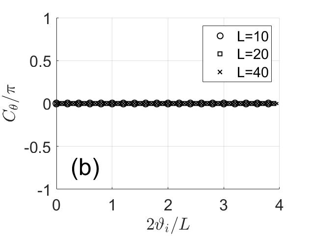
(b)

Figure 10: The values of the correction term in Eq.(30), $C_{\theta}=\frac{1}{L^{3}}\sum_{M_{i}=0}^{N}\left|\frac{\sin\frac{L\tilde{\theta}_{M_{i}}}{2}}{\sin\frac{\tilde{\theta}_{M_{i}}}{2}}\right|^{2}\tilde{\theta}_{M_{i}}$. (a) $\theta_{i}^{(0)}$ is fixed at $-\pi/L$. (b) $\theta_{i}^{(0)}$ is changed to keep all the $\tilde{\theta}_{M_{i}}$ lie in the region of $[-\pi,\pi)$. Two periods of $\vartheta_{i}$ are plotted in these two figures.

We can understand this question from another point of view. Since expectation values of well 1 and 2 are independent of each other, we may ignore the degrees of freedom related to well 2 and consider a reduced double-well case. Note that $\theta_{1}$ is actually a periodic quantity, and we should actually plot the amplitude $|\langle\theta_{M_{1}}|\ell_{1},\vartheta_{1}\rangle|^{2}$ on a ring. Therefore, different choice of $\theta_{1}^{(0)}$ turns out to represent cutting the ring at different positions, as illustrated by Fig.11. Obviously Fig.11a will have a slightly larger expectation value of $\hat{\theta_{1}}$ than Fig.11b, but as long as the cut is not in the peak, whose width scales as $O(L^{-1})$, the deviation will be small. This is the origin of the correction term in Eq.(30).

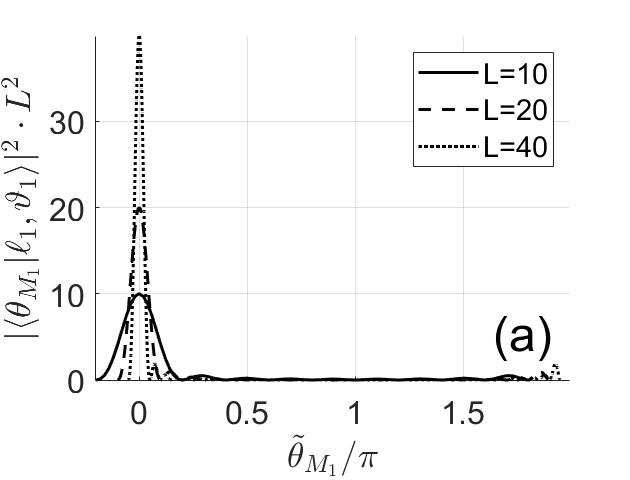
(a)

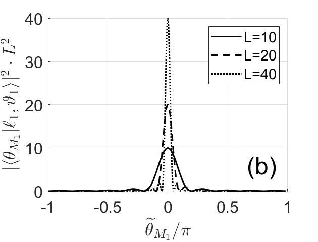
(b)

Figure 11: $|\langle\theta_{M_{1}}|\ell_{1},\vartheta_{1}\rangle|^{2}$ versus $\tilde{\theta}_{M_{1}}$, with fixed $\vartheta_{1}=0$ and different choice of $\theta_{1}^{(0)}$. (a) $\theta_{1}^{(0)}=-\pi/L$. (b) $\theta_{1}^{(0)}=-\pi$.

If we allow $\theta_{1}^{(0)}$ to change with the shifting of $\vartheta_{1}$ and keep all the $\tilde{\theta}_{M_{1}}=\theta_{1}^{(0)}+2\pi M_{1}/L^{2}-2\pi\vartheta_{1}/L$ ($M_{1}=0,1,...,L^{2}-1$) lie in the region of $[-\pi,\pi)$, as in Fig.11b, then the peak in $|\langle\theta_{M_{1}}|\ell_{1},\vartheta_{1}\rangle|^{2}$ will always be at the middle point of the region, hence the correction term will be exactly 0 for arbitrary $\vartheta_{1}$, as shown in Fig.10b.

A.3 Localization of the Planck cells

Finally, we analyze the fluctuations of these expectation values, i.e. the localization of the shapes of these Planck cells. The fluctuations are

$$\Delta n_{i} = \frac{\sqrt{\langle\hat{N_{i}}^{2}\rangle_{\ell_{i},\vartheta_{i}}-\langle\hat{N_{i}}\rangle_{\ell_{i},\vartheta_{i}}^{2}}}{N}$$ (32)

$$=\frac{1}{\sqrt{12N}}\sim\frac{1}{\sqrt{12}L},$$

$$\Delta\theta_{i} = \sqrt{\langle\hat{\theta_{i}}^{2}\rangle_{\ell_{i},\vartheta_{i}}-\langle\hat{\theta_{i}}\rangle_{\ell_{i},\vartheta_{i}}^{2}}$$ (33)

$$= \sqrt{\frac{1}{L^{3}}\sum_{M_{i}=0}^{N}\left|\frac{\sin\frac{L\tilde{\theta}_{M_{i}}}{2}}{\sin\frac{\tilde{\theta}_{M_{i}}}{2}}\right|^{2}\tilde{\theta}_{M_{i}}^{2}-C_{\theta}^{2}}\,.$$

As discussed above, we can choose $C_{\theta}=0$ so that Eq.33 can be further estimated as

$$\Delta\theta_{i} \sim \sqrt{\frac{1}{L^{3}}\int_{-\pi}^{\pi}\mathrm{d}x\cdot L^{2}\cdot\left|\frac{\sin\frac{Lx}{2}}{\sin\frac{x}{2}}\right|^{2}x^{2}}$$

$$= \sqrt{\frac{1}{L^{3}}\int_{-\pi}^{\pi}\mathrm{d}x\cdot L^{2}\cdot\sin^{2}\frac{Lx}{2}\frac{x^{2}}{\sin^{2}\frac{x}{2}}}$$

$$\sim \sqrt{\frac{A}{L}\int_{-\pi}^{\pi}\mathrm{d}x\cdot\sin^{2}\frac{Lx}{2}}$$

$$\sim \sqrt{\frac{\pi A}{L}}$$

where $A$ is a constant of order $O(1)$ introduced due to the fact that $x/\sin(x/2)\sim O(1)$ over the entire region of $[-\pi,\pi)$. Therefore, for both the particle number and the phase, the fluctuations of the expectation values converge to 0 as $L$ goes to infinity. This establishes the localized ‘cell’ picture of each Planck cell.

Appendix B Examples of computing the Wasserstein distance

We use two examples to compute the Wasserstein distance between distributions. We consider two distributions

$$p_{A}(x)=\begin{cases}1/5&x<5\\ 0&x\geq 5\end{cases}$$ (35)

and

$$\ p_{B}(x)=\begin{cases}1/5&x\text{ is even}\\ 0&\text{otherwise}\end{cases}$$ (36)

on the set $\mathcal{B}=\{0,1,\cdots,9\}$. We want to compute the Wasserstein distance between them and the uniform distribution. We choose the metric on $\mathcal{B}$ as $d(x,y)=|x-y|\ ;\ x,y\in\mathcal{B}$. The Wasserstein distance can be computed as follows.

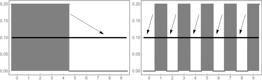
Figure 12: The most efficient way to achieve the transport between two distributions.

The transport matrix between $p_{A}$ and uniform distribution $p_{E}(x)=1/10$ is $P_{ij}\in[0,1]$, which obeys

$$\sum_{j\in\mathcal{B}}P_{ij}=p_{A}(i)\ ;\ \sum_{i\in\mathcal{B}}P_{ij}=p_{E}(j)$$ (37)

The Wasserstein distance for $\lambda=1$ is the minimum value of

$$\sum_{i,j\in\mathcal{B}}P_{ij}d(i,j)\,.$$ (38)

This shows that the Wasserstein distance is the most efficient way to transform one distribution to another. As both distributions $p_{A}$ and $p_{B}$ are simple, the most efficient ways are shown in Fig. 12. For the distribution $p_{A}$, the non zero optimal $P_{ij}^{*}$ are

$$P_{i,i}^{*}=P_{i,i+5}^{*}=1/10\ ;\ i=0,1,\cdots,4$$ (39)

which means the Wasserstein distance: $D_{1}(p_{A},p_{E})=5\times|5-0|\times 1/10=2.5$. Similarly, we have $D_{1}(p_{B},p_{E})=5\times|1-0|\times 1/10=0.5$.