LSQT: Low-Stretch Quasi-Trees
for Bundling and Layout

Abstract

We introduce low-stretch trees to the visualization community with LSQT, our novel technique that uses quasi-trees for both layout and edge bundling. Our method offers strong computational speed and complexity guarantees by leveraging the convenient properties of low-stretch trees, which accurately reflect the topological structure of arbitrary graphs with superior fidelity compared to arbitrary spanning trees. Low-stretch quasi-trees also have provable sparseness guarantees, providing algorithmic support for aggressive de-cluttering of hairball graphs. LSQT does not rely on previously computed vertex positions and computes bundles based on topological structure before any geometric layout occurs. Edge bundles are computed efficiently and stored in an explicit data structure that supports sophisticated visual encoding and interaction techniques, including dynamic layout adjustment and interactive bundle querying. Our unoptimized implementation handles graphs of over 100,000 edges in eight seconds, providing substantially higher performance than previous approaches.

1 Introduction

Graph visualization poses many challenges, most of which become increasingly problematic as a graph’s size increases [42]. One of the greatest challenges in graph visualization occurs when a large graph display is too cluttered to interpret or explore. Two main approaches for taming this graph complexity problem, the so-called hairball problem, exist in the current visualization literature: first, developing novel layouts to find better spatial positions for nodes and edges; second, developing novel edge-bundling approaches to group edges together and reduce visual clutter. These approaches have typically been approached separately. Here, we introduce a technique that addresses both of them.

In this work, we revisit the idea of quasi-trees, which had previously been used only for graph layout, by showing their utility for edge bundling. Intuitively, a quasi-tree is any tree extracted from a graph that is used as a representative proxy for the full graph. For example, one previous quasi-tree approach uses a backbone of spanning tree edges as the skeleton for a graph layout, where node positions are determined by a tree layout algorithm and the edges included in the tree are straightforward to draw [35]. The non-tree edges, called remainder edges, are excluded from the layout process that determines node positions but can be routed according to the backbone of the tree, and can then be drawn or hidden on demand. Our new idea is to use these remainder edges to explicitly compute a data structure of bundles.

We accomplish these advances through the use of low-stretch trees, a mathematical formalism that exposes underlying hierarchical structure in relational datasets [4]. Importantly, low-stretch trees can be used to find tree structure in any graph, even those that do not have apparently tree-like characteristics. We propose low-stretch trees as a useful tool for the graph visualization community, and use them to help expand the reach of quasi-tree methods beyond their previously limited scope of obviously tree-like sparse graphs.

We offer two contributions to the graph visualization literature. Our first contribution is the introduction of low-stretch trees for graph visualization, which allows us to expand the scope of quasi-tree methods beyond their previously assumed limits. Our second contribution is the novel LSQT algorithm for bundling and layout using low-stretch quasi-trees. The bundles are explicitly computed from the graph topology before any geometric layout occurs. This algorithm segments remainder edges into bundles using efficient queries on paths within the quasi-tree, leading to algorithmic speed and quality guarantees because the quasi-trees that it computes are low-stretch. We demonstrate an implementation of this algorithm in a simple proof-of-concept interactive viewer.

2 Quasi-Tree Rationale

We provide background on quasi-tree approaches to layout and discuss the implications of extending these ideas to edge bundling.

2.1 Layout

Four major families of layout methods dominate the previous graph visualization literature: force-directed [26], geographic [12], cluster-based [19, 14], and adjacency matrix [23] views. A fifth family of layout methods, quasi-trees, does exist but is currently under-appreciated, with only a few examples in the existing literature such as H3 [35], SPF [6], and the focus-based filtering approach of Boutin et al. [11]. Quasi-tree layout methods extract a hierarchical structure, specifically a spanning tree, from a general graph. Every graph node is a tree node and edges are split into two classes: backbone edges within the spanning tree ($E_{T}$), which are used to drive the node layout, and remainder edges ($E_{R}$), which are all edges not in the tree. Formally, for a graph $G=(V,E)$, the remainder edges $E_{R}$ = $E\ E_{T}$. For example, a previous two-phase approach [35] first uses standard tree layout algorithms to lay out all of the nodes and the backbone links, and then routes the remainder edges in a second pass using the computed node positions. An alternative is to use standard force-directed placement for the entire graph [11].

The remainder edges will typically cause significant visual clutter, since the resulting layout is not optimized to avoid those edges crossing the backbone edges or the node positions. The simple clutter mitigation strategies proposed in previous work include interaction techniques where remainder edges are drawn only on demand for the edges incident to a selected node or subtree, and visual encoding techniques where remainder edges are drawn differently from backbone edges [35].

Using a quasi-tree layout would be misleading for users if the imposed hierarchical layout does not adequately capture the graph’s true structure, because the clutter reduction strategies would hide important information about that structure rather than secondary details. Clearly quasi-tree layouts are suitable when graphs have near-tree, sparse structure leading to only a small proportion of remainder edges compared to backbone edges. Past work by Archambault et al. [6] does propose quasi-tree layouts for de-cluttering dense graphs in a “last-ditch” context where other layout approaches result in uninterpretable hairball problems. Inspired by the potential of quasi-trees to tame visual clutter, we argue that these methods are a viable first choice when we use low-stretch trees because they capture true structure even in graphs that are not obviously trees. Our approach shows the suitability of quasi-tree methods for de-cluttering a much larger class of graphs than previously understood.

2.2 Bundling

Beyond layout, we argue that quasi-tree methods are viable approaches to taming graph complexity with edge bundling. We propose a novel bundling system, where backbone edges of a tree are not bundled. Instead, only the remainder edges are bundled, and we explicitly compute these bundles in order to store them in a data structure that can be exploited by visual encoding and interaction techniques. We subdivide the remainder edges into segments, which can then be routed according to the existing backbone edge structure. Segments with shared endpoints are collected into bundles. We adopt the useful terminology of routing graph from Bouts and Speckmann [13], meaning the scaffolding for determining the position of the remainder edges.

Another implication of our quasi-tree approach to bundling is that it allows the bundling computation to occur before any geometric layout, because it is based only on the graph’s topology. Our approach allows complete independence from the layout when bundling: no initial geometric layout is required. This approach is particularly suitable when a graph layout has not already been computed, or an existing graph layout is either unintuitive (for example, a geographic layout that is a mismatch for a topologically focused task), or uninterpretable (for example, a hairball where the geometry does not capture the topological detail). It is important to note that our method is unsuitable if there is an existing graph layout that captures useful structure in the data given an intended task. In this case, previous methods that strive to preserve the original layout [30, 8, 37] are a better choice.

Just as quasi-tree approaches to layout strongly prioritize clutter removal, quasi-tree bundling approaches are an aggressive approach to de-cluttering. They are similar in spirit to ink minimization edge bundling approaches [27, 20], which prioritize de-cluttering. In contrast, other families of approaches such as image-based or geometry-based bundling [20, 13, 38] have the goal of preserving the original graph layout.

3 Low-Stretch Quasi-Trees

We define low-stretch trees and explain their properties, discuss the algorithm for extracting them from a graph and its complexity, and present an analysis of their suitability for our purposes.

3.1 Definition and Guarantees

Low-stretch trees have been developed in the theoretical computer science community over the past twenty five years. They are related to the notion of spanners, which have been studied in the graph theory community for many decades [4]. A spanner can be defined as a subgraph that approximately preserves edge distances. Given a graph and a spanning tree, the stretch [4] is the ratio between path length in the tree and path length in the original graph. A low-stretch tree is a spanning tree that approximately minimizes the stretch of edges on average. Such a tree provides a desirable preservation of distance for the creation of a good routing graph that is used to lay out the remainder edges. These trees are the key objects underlying several recent breakthroughs in spectral graph algorithms, such as maximum flow in near-linear time [41], but they have yet to be exploited for graph visualization.

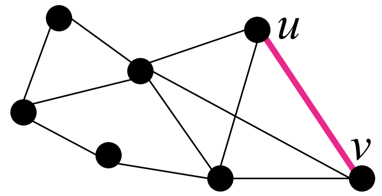
(a) Original graph $G$, with comparison edge $e=(u,v)$ highlighted

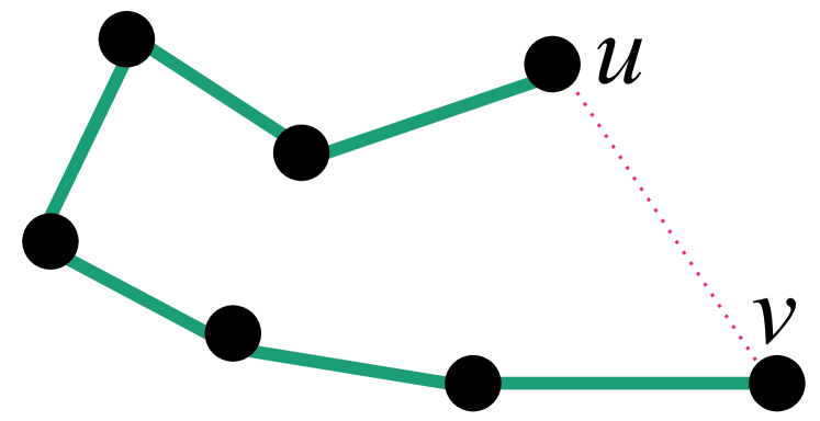
(b) Tree $T$ with $s_{T}(e)=6$, $s_{T}(G)={28}/{11}$

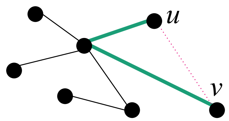
(c) Tree $T$ with $s_{T}(e)=2$, $s_{T}(G)={17}/{11}$

Figure 1: Comparison between trees with poor (high) and good (low) stretch, respectively.

Figure 1 gives an example of two spanning trees: one with poor (large) stretch, and one with good (small) stretch. For graph $G=(V,E)$, the stretch of an edge $e=(u,v)\in E$ in tree $T$ is defined as:

$$s_{T}(e)=d_{T}(u,v)$$

where $d_{T}(u,v)$ is the path length from $u$ to $v$ in $T$. The overall stretch of $G$ is defined as:

$$s_{T}(G)=\frac{1}{|E|}\sum_{e\in E}s_{T}(e)$$

Low-stretch trees are considerably more effective at capturing the structure of general graphs than typical spanning trees. Their power can be illustrated through a simple example in Figure 2. Consider a square grid graph, or mesh, with $n$ vertices. Arbitrary spanning trees generally do a poor job of capturing the structure of this graph, as in the example of the comb shaped tree in Figure 3a. For any vertical edge in the right half of the grid, the endpoints of that edge are at distance 1 in the original graph, but they are at distance $\Omega(\sqrt{n})$ in the tree because the unique path through the tree connecting those two vertices traverses all the way to the left-most column. It is by no means obvious whether any subtree of the grid graph can have substantially better stretch. Alon et al. [4] pointed out that the grid contains a fractal-like subtree with stretch $O(\log n)$, shown in 2(b), that is reminiscent of Hilbert’s space-filling curve [24]. They also show that the logarithm is necessary: every spanning tree of an $n$-vertex square grid has stretch $\Omega(\log n)$. Therefore, low-stretch trees provide an opportunity to vastly improve utility of quasi-tree based methods due to provable guarantees of minimizing structural discrepancies.

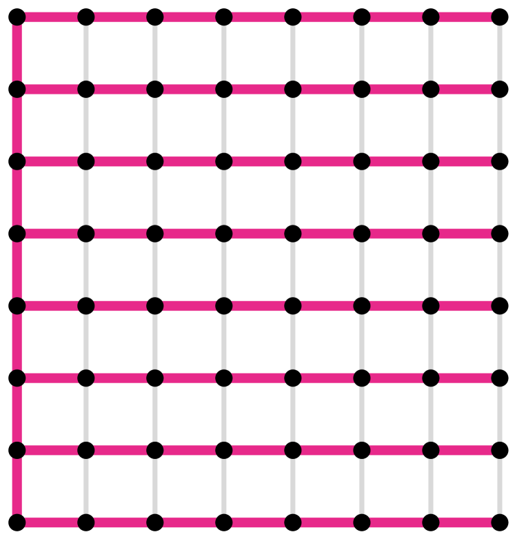
(a) A spanning tree.

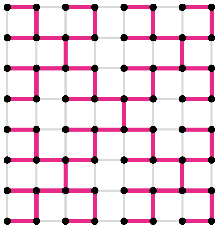
(b) Low-stretch spanning tree, as shown in Alon et al. [4].

Figure 2: Comparison between an arbitrary spanning tree and a low-stretch spanning tree for an 8-by-8 grid graph.

3.2 Extracting Low-Stretch Trees From a Graph

In order to extract a low-stretch tree from an existing graph, we can simply use the existing algorithm from Alon et al. [4]. This algorithm performs an iterative coarsening process in order to compute the low-stretch tree. At each step of the algorithm, vertices are partitioned into clusters. Each of these clusters has low topological diameter. Next, a shortest-paths spanning tree is computed for each cluster. The edges from these trees are added to an (initially empty) low-stretch tree, and each cluster is then contracted into a meta-vertex. Edges are then added to represent connections between vertices in different clusters. The algorithm then iterates on this new multigraph.

3.3 Complexity Analysis

The low-stretch tree construction algorithm from Alon et al. [4] runs in time $O(m\log n)$, where $m$=$|E|$ and $n$=$|V|$. The tree is guaranteed to have low average stretch: $\exp(O(\sqrt{\log n\log\log n}))=O(n^{0.01})$. Note that $n^{0.01}$ is very small: it is 1.12 for a graph of one million vertices. Other methods with better theoretical guarantees are known [1, 16], but their algorithms are not practical to implement. A new method claims to have faster running time of $O(m\log n\log\log n)$ [2], but it is unclear whether this approach is practical. Regardless, any method can be substituted to compute the low-stretch tree in this step, provided there are guarantees on the stretch of the resulting tree.

3.4 Assessing Bundle Quality

Computing a low-stretch quasi-tree backbone addresses two requirements for edge bundling proposed in previous work [13, 38]: short paths are desirable when bundling edges and sparsity is important for spanners used to route edge bundles. As we explain in Section 3.1, low-stretch trees offer provable path-shortness guarantees, addressing the first criterion, and our LSQT algorithmic approach is provably sparse compared to arbitrary spanners, addressing the second one.

4 Related Work

Our algorithm combines the previously distinct spaces of graph layout and bundling approaches, and introduces low-stretch trees to the visualization literature.

4.1 Layout

Quasi-tree layouts have received only limited attention in the previous work; they have not even been considered a major category by previous graph visualization surveys [34, 36]. An early example is the interactive H3 system [35] that extracts a spanning tree from a general graph and uses it for layout. The backbone edges are drawn at all times using fully custom tree layout that exploits the mathematical properties of hyperbolic geometry. The remainder edges can be toggled on or off for individual nodes, all nodes within a subtree, or the entire graph. Boutin et al. [11] use the combination of filtering and clustering to extract a “tree-like graph” and use that quasi-tree either to guide a standard force-directed layout algorithm or as input for their customized multi-level silhouette tree layout. The LGL system uses a spanning tree as a skeleton to guide their variant of force-directed layout for general graphs [3]. The multi-stage static SPF layout algorithm [6] uses an input spanning tree as an initial skeleton in an extended version of LGL at one of its stages.

Bourqui and Auber [10] use a more sophisticated clustering-based approach to extracting quasi-tree structure from a graph in order to draw large quasi-trees at higher quality than SPF. Giot and Bourqui [22] introduce more efficient algorithms for both extracting appropriate quasi-tree structure and a custom bottom-up area-aware layout. These two algorithms are similar to our own work since they both include a final bundling stage to reduce clutter, based on Holten’s HEB approach [25]. Although they do combine layout and bundling for quasi-trees, their fundamental emphasis is on bundling to improve the layout of quasi-trees in specific, whereas ours is to use quasi-trees to drive a bundling algorithm for general graphs.

4.2 Bundling

Edge bundling approaches fall into three major families: image-based, geometry-based, and cost-based bundling. Image-based bundling [17, 43] uses processes like splatting and shape skeletonization on previously computed bundling layouts (from either cost-based or geometry-based approaches) to build new shaded shapes used for visualizing each set of edges. Geometry-based bundling [15, 39] employs spatial decomposition using spatial data structures such as quadtrees, uniform or non-uniform grids, or triangle meshes to determine the shape and curve of the edges in the display. Cost-based bundling [28, 20] is named based on the metaphor of saving the cost of ink, and more generally includes all energy minimization approaches. LSQT falls into this category. The shapes of the edges are determined by the cost of ink, or energy, it will take to draw the edges. Multilevel agglomerative edge bundling (MINGLE) [21] is one example of an ink-saving strategy. Force-directed edge bundling methods [26] are all examples of energy minimization approaches, which focus on reducing the spring energy associated with the models used to draw a given system [21]. Cost-based approaches typically aim for aggressive de-cluttering over maintaining the interpretability of the existing spatial topology.

Three cost-based approaches are most similar to our own. One is the seminal edge bundling proposal, Hierarchical Edge Bundling (HEB) [25], which does not rely on an existing layout; we call this property layout agnostic. Surprisingly, despite the enormous amount of followup work on edge bundling, no later methods extended this aspect of the work. Instead, the many examples [28, 27, 17, 39, 20, 31, 13, 38] of subsequent methods for bundling are in the category we call layout first, where they rely on an existing layout in order to compute bundles. To the best of our knowledge we are the first to continue exploring the benefits of layout-agnostic approach, which avoids the computational expense of a preprocessing step to create an initial graph layout and allows users to explore multiple possible layout approaches for the underlying quasi-tree structure without the need to recompute bundles.

Kernel Density Estimation Edge Bundling (KDEEB) [28] is a cost-based layout-first approach that improved upon several documented computational complexity issues with other algorithms for general graphs by providing a robust and simple approach, with an implementation that performs faster than most other algorithms. Edges are advected along a density map to create a layout with smooth and well-separated bundles. The visual results are notably different than many other edge bundling approaches, so direct comparison to previous methods is difficult. The authors argue that a useful quality heuristic is to have areas of clear separation between high-density bundles where the edges are densely packed, given the goal of minimizing ink [28]. Our LSQT approach takes a similarly aggressive approach to de-cluttering, and also yields results quite visually different from previous methods.

Clustered Edge Routing (CER) [13] is also a cost-based, layout-first approach. It is the most similar approach to LSQT in terms of using a sophisticated mathematical formalism to compute spanners, well-separated pair decomposition, in order to achieve aggressive de-cluttering of graph visualizations. The authors quantify several desirable properties of a routing graph, and two of them can be applied to our layout-agnostic approach: sparsity is crucial for routing graphs, and the shortest path between two vertices in the routing graph should not be much longer than their direct connection in the graph. In our work, we use these properties as guidelines for the characterization of desirable properties of spanners for bundle routing. Specifically, our low-stretch spanning tree has provable guarantees of sparsity that are stronger than the limited guarantees provided by their method of computing spanners: to preserve distance with a multiplicative factor $O(t)$, it is known that $\Omega(n^{1+1/t})$ edges are needed [5]. Also, the complexity of their method is $O(n^{2}\log n)$; we have clear speed advantages, in that both the computational complexity and the empirical performance of our algorithm are superior.

4.3 Low-Stretch Trees

The mathematical formalism of low-stretch trees [4] arose in the theoretical computer science community where it has been applied to the construction of spanners, but has not been previously introduced in the visualization or graph drawing literature.

5 Quasi-Tree Bundling Algorithm

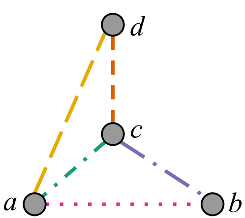
(a)

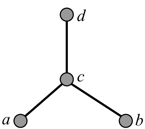
(b)

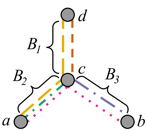
(c)

Figure 3: LSQT bundling algorithm. A low-stretch tree $T=(V,E_{T})$ is computed for use as a routing graph. Segmentation is performed by routing edges through this tree, as illustrated in Figure 4. Bundles are then formed from groups of segments sharing the same endpoints as edges in $E_{T}$. (a) Original graph $G$, where colour and dash style are used to differentiate edges. (b) Routing tree $T$. (c) Result showing three bundles, where segments have the same visual encoding as above.

(a)

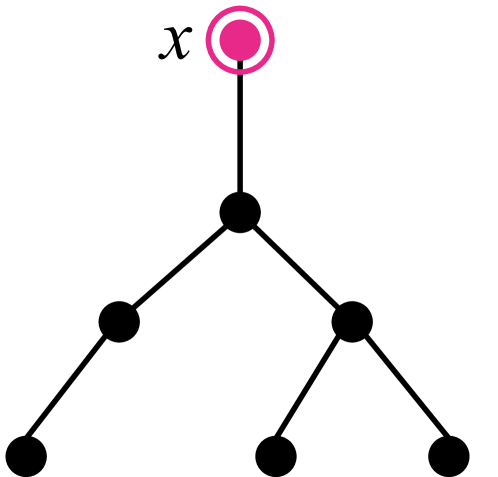
(b)

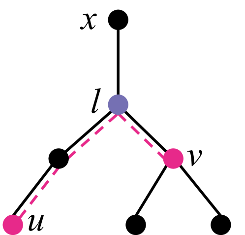
(c)

Figure 4: LSQT routing algorithm. The tree $T=(V,E_{T})$ is rooted at an arbitrary vertex in order to speed up queries, which then only need to find the lowest common ancestor between two vertices. (a) Original (unrooted) tree $T$. (b) $T$ rooted at arbitrary vertex $x$. (c) To find the path from $u$ to $v$ in $T$, we find their lowest common ancestor, $\ell$, by climbing up the tree. The path from $u$ to $v$ is then the concatenation of paths $u\text{-}\ell$ and $\ell\text{-}v$.

Our method computes bundles directly, without relying on the geometry of vertices or edges. We route edges through a tree to determine both edge segmentation and bundle membership. The algorithm consists of two steps: routing graph generation, where the spanning tree is computed; and edge routing, where edges are segmented and bundles are formed. We first detail how to segment remainder edges, and then explain how our process allows for subsequently efficient path queries in the routing process. Finally, we present a complexity analysis for LSQT.

5.1 Efficient Segmentation

We will use a low-stretch tree as our routing graph for bundling. We compute this tree using the algorithm proposed by Alon et al. [4]. It performs an iterative coarsening process in order to compute the low-stretch tree. We subdivide each remainder edge into segments that follow the backbone quasi-tree vertex structure. We bundle only these remainder edges, and each remainder edge is represented by an ordered list of segments. This process is illustrated in Figure 3.

At each step of the algorithm, the vertices of the graph are partitioned into clusters such that each cluster has low topological diameter. A shortest-paths spanning tree is then computed for each cluster, and the edges from these trees are added to the (initially empty) low-stretch tree. Each cluster is then contracted into a meta-vertex, and edges are added to represent connections between vertices in different clusters. The result is a multigraph, where a single node may share multiple edges. This multigraph contains only quasi-tree edges, where the nodes are vertices from the original graph. The multigraph is used to create bundles, which are simply defined as a set of two or more segments with the same endpoints. LSQT then iterates on this new multigraph. Segments in the same bundle are referred to as bundle neighbors. The construction of these segments is thus purely topological and does not depend on geometric layout.

To perform segmentation and bundling efficiently, we query $u\text{-}v$ paths in our spanning tree $T$. We need a fast subroutine to handle this procedure. A naïve approach is to simply perform breadth-first search, but that would require $\Theta(|V|)$ time per query. Since $\Omega(|E_{R}|)$ queries are needed, where $E_{R}$ are the remainder edges, this approach requires $\Omega(|V|\cdot|E_{R}|)$ time. Instead, we will use a two-phase approach that pre-processes the graph in linear time, but can then perform queries in time proportional to the length of the returned path (which is optimal, as the path itself is returned). Performing such a query for every remainder edge in $E_{R}$ requires time $O(s_{T}(G)\cdot|E_{R}|)$, which is small since $T$ is a low-stretch tree.

This subroutine can be easily implemented as follows. The pre-processing step simply roots the tree at an arbitrary vertex and directs all edges towards the root. Then, to find a $u\text{-}v$ path in $T$, step in parallel from each of $u$ and $v$ towards the root, marking the nodes along the way. The first marked vertex encountered on either path is the lowest common ancestor $\ell$, and the time to identify it is proportional to the length of the $u$-$v$ path. The path through the tree is then the concatenation of paths $u\text{-}\ell$ and $\ell\text{-}v$, and the segmentation of $(u,v)$ is this path. This process is illustrated in Figure 4. Once the $u\text{-}v$ paths have been computed for each $(u,v)$, bundles are formed such that all segments that have the same endpoints are bundle neighbours.

5.2 Complexity Analysis

The query time to identify the least common ancestor (LCA) is proportional to path length. As stated in Section 3.3, the time to compute the low-stretch tree is $O(m\log n)$ where $m$=$|E|$ and $n$=$|V|$. As observed above, the total time for querying the low-stretch paths for every remainder edge in $E_{R}$ requires time $O(s_{T}(G)\cdot|E_{R}|)=O(m*n^{0.01})$.

6 Visual Encoding and Interaction Possibilities

In this section, we discuss a proof-of-concept viewer to demonstrate visual encoding possibilities enabled by the LSQT algorithm. We take advantage of the key assets of our bundling algorithm when designing the visual encodings for LSQT: namely, that it does not require a pre-determined layout, and that it creates the data abstraction of bundles that are directly accessible through their own data structure. The viewer supports interactive queries of the bundle structure, and also allows arbitrary layout adjustment through dragging.

6.1 Quasi-Tree Layout Approaches

Because LSQT computes bundles before layout, we can position the vertices in any way we choose. For example, we can use any layout for the low-stretch tree backbone. 5(a) and 5(b) show a proof-of-concept viewer using two popular layout approaches: the standard force-directed graph layout that is built into D3 [9], and the standard Reingold-Tilford tree drawing approach [40]. Future work could use any previously proposed or custom-designed tree drawing approach, since the LSQT backbone is itself a tree.

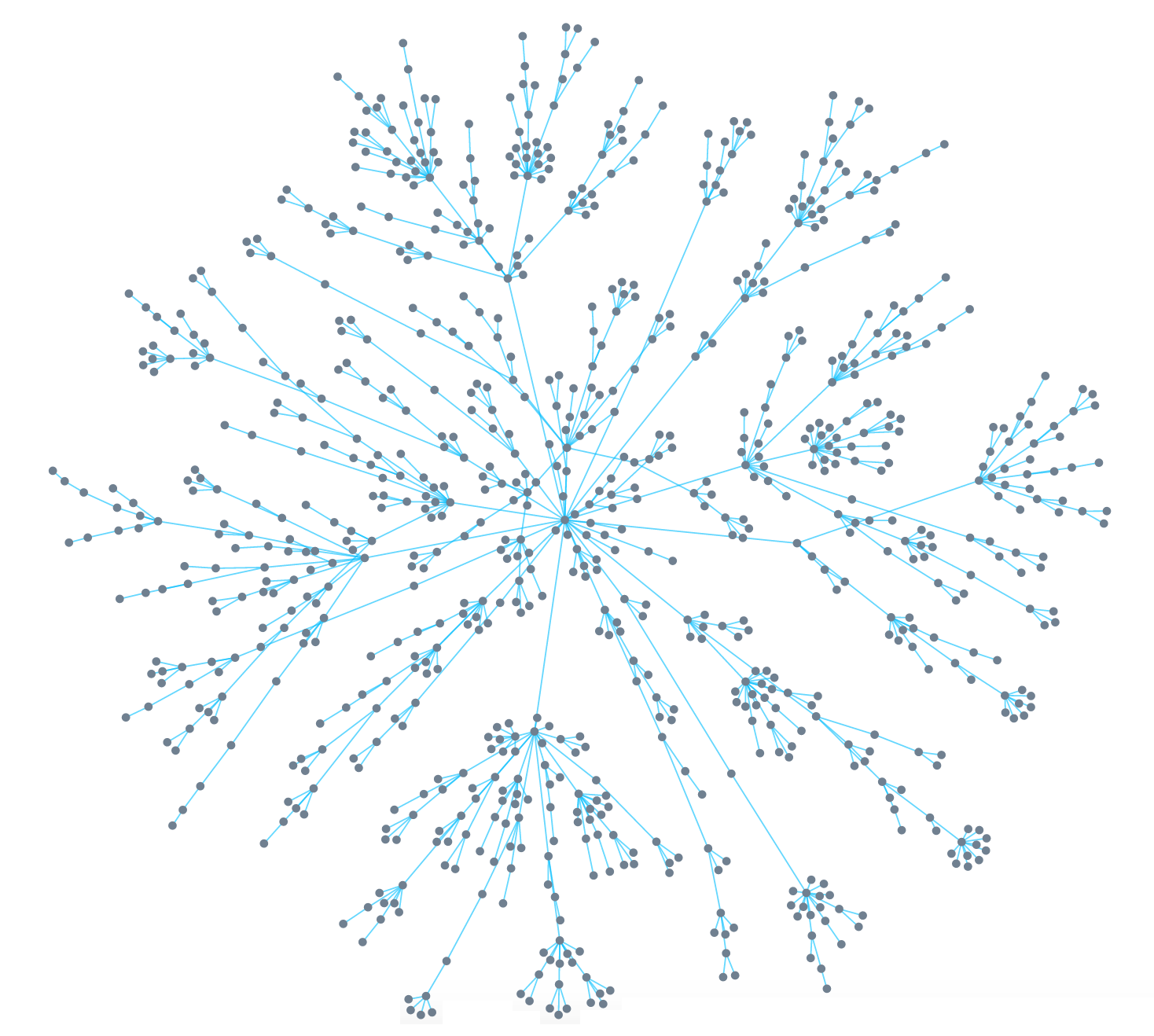
(a) Force-directed layout

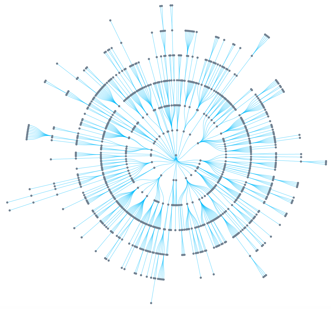
(b) Radial Reingold-Tilford layout

Figure 5: Comparison between two common vertex layout possibilities for the LSQT routing graph $T$.

6.2 Encoding and Interaction

In addition to the layout, there are remaining design choices for visual encoding and interaction.

6.2.1 Bundle Visual Encoding

We draw bundles explicitly, both independently from and in combination with individual drawing of remainder edges. Figure 6 shows the different visual encoding options for bundles and edges. Bundles are depicted by straight lines with tapered endpoints and varying thickness, as shown in 6(a). The thickness of bundles varies in proportion with bundle size (the number of segments in a bundle). Individual edges are drawn as splines, as shown in 6(b). The control points for the spline of edge $(u,v)$ are the endpoints of its segments, which correspond to the vertices in the $u\text{-}v$ path in $T$. This approach is similar to the method of HEB [25]. Bundles and edges can also be drawn simultaneously, where distinct perceptual layers are created by adjusting opacity. 6(c) and 6(d) show the difference between having bundles and remainder edges as the foreground layer.

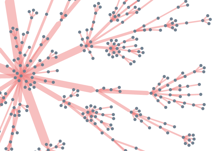
(a) Bundles only

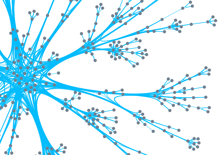
(b) Remainder edges only

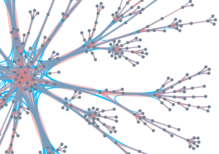
(c) Bundles foreground

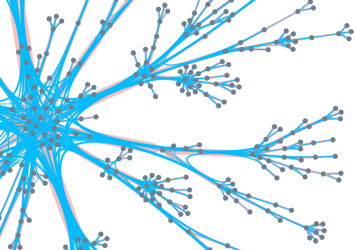
(d) Remainder edges foreground

Figure 6: Examples of visual encoding options for LSQT.

6.2.2 Interaction Idiom Examples

In our proof-of-concept viewer, vertices can be re-positioned by the user with interactive dragging, without the need to re-run the edge bundling algorithm. Previous bundling methods would not support this style of interaction because their bundling is dependent on a static and pre-computed layout. The viewer also supports interactive exploration of the mapping between edges and bundles. 7(a) shows hovering over a bundle in order to highlight all edges belonging to that bundle in the viewer. Figure 7(b) shows single edges individually highlighted on hover.

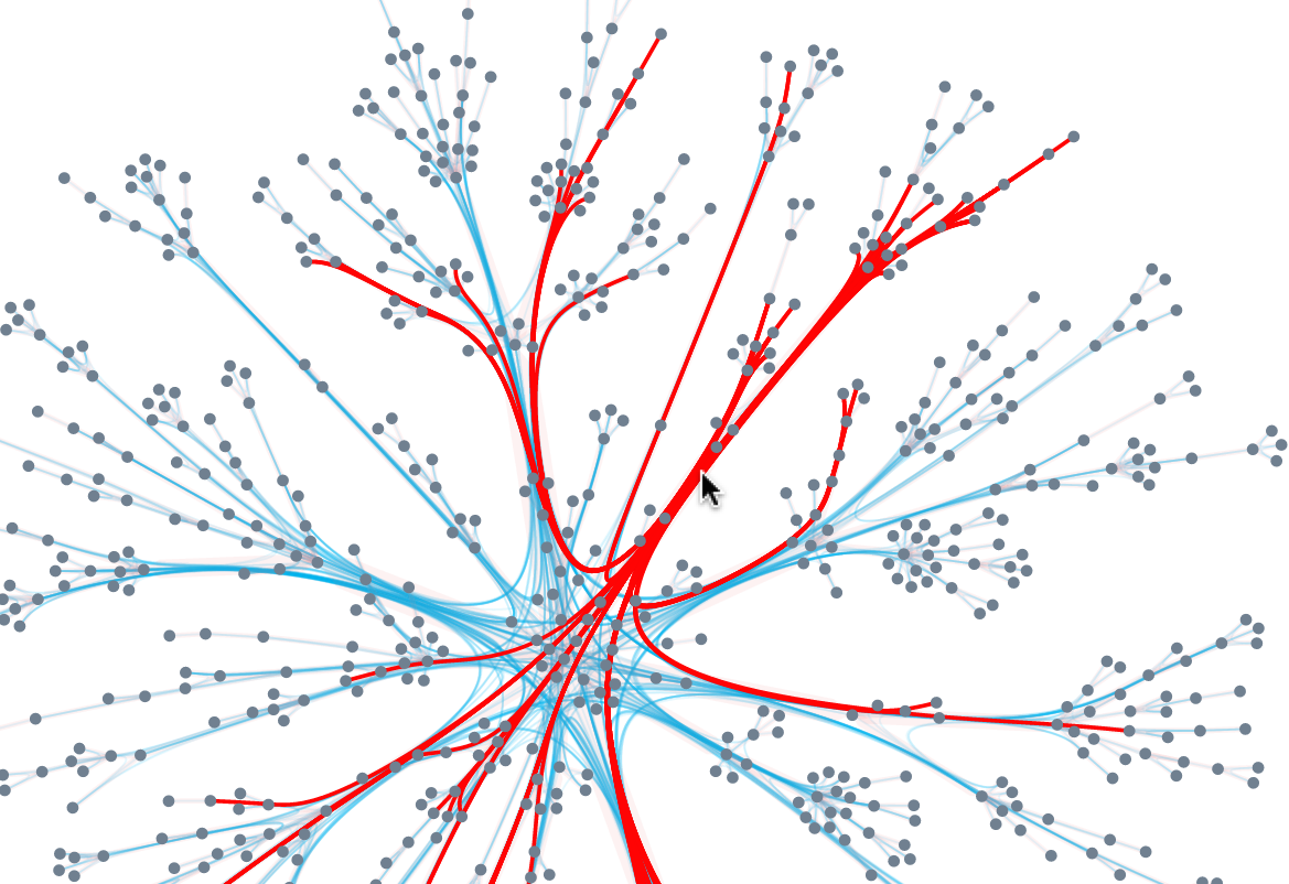
(a) Hovering over a bundle highlights edges in that bundle

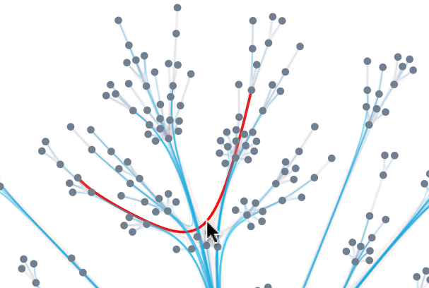
(b) Hovering over an individual edge highlights that edge

Figure 7: Comparing bundle querying and edge querying.

6.2.3 Visual Layering

Users can choose to display one of three modes: bundles alone, remainder edges alone, or a combination of bundles and remainder edges simultaneously. Distinct perceptual layers are created by adjusting the opacity when drawing bundles/backbones and remainder edges simultaneously. Additionally, users can switch between bundles and remainder edges as the foreground layer.

7 Results

We present results using datasets that have been used in previous work; we chose them to enable comparisons between existing methods, based on their popularity in cited literature and diversity among layout and bundling style. Table I lists the five graphs, along with size statistics (number of vertices and edges) and a brief description.

dataset	$|V|$	$|E|$	Description
Flare	220	708	Software hierarchy
Poker	859	2127	Poker game graph
Email	1133	5451	Email interchange
Yeast	2224	6609	Protein interaction
Wiki	7066	100736	Wikipedia elections

TABLE I: Graph statistics for datasets used in this paper.

dataset	$|V|$	$|E|$	LSQT	Bundle	Draw	Total
Flare	220	708	0.022	0.005	0.032	0.060
Poker	859	2127	0.082	0.026	0.108	0.216
Email	1133	5451	0.180	0.053	0.283	0.516
Yeast	2224	6609	0.247	0.070	0.342	0.659
Wiki	7066	100736	4.275	1.010	2.782	8.067

TABLE II: Performance statistics of LSQT. Running time is in seconds, and is averaged over 100 runs.

7.1 Implementation

LSQT is implemented in Python and JavaScript, using D3 [9] for drawing. Our code is open-source and available at https://github.com/rebvan/lsqt. Our proof of concept viewer can be found at https://lsqt-vis.herokuapp.com. All results in this paper are from runs on a MacBook Pro with a 2.6 GHz Intel Core i7 and 16 GB of 1600 MHz DDR3 RAM.

7.2 Computational Performance

Table II shows performance statistics of LSQT, breaking down the total computation time into three phases: computing the low-stretch backbone, computing the bundles and their data structure, and drawing the graph using the standard D3 force-directed drawing. Running times for LSQT range from 0.06 seconds for a graph with over 700 edges to just over 8 seconds for graph of over 10,000 edges. On this large graph, the MINGLE paper reports a running time of 18.4 seconds, albeit on an older architecture [21]; it is the fastest previous method, and we achieve competitive performance with our proof-of-concept implementation that uses an unoptimized scripting languages. In contrast, MINGLE is implemented in C using OpenGL on a GPU, leading us to believe that LSQT speed could be substantially improved with a GPU port or simple optimization techniques.

7.3 Qualitative Layout Comparison

In this section, we qualitatively compare visual encodings computed with LSQT to encodings of the same data from five previous bundling and layout methods, as shown in Figure 8. Four of the methods are layout-first, and we directly show images from those previous papers: KDEEB [28], CER [13], MINGLE [21], SBEB [18]. For the fifth method, the layout-agnostic HEB [25], we created a screenshot using the D3 package that implements this algorithm.

\begin{overpic}[width=130.08731pt,trim=0.0pt 0.0pt 0.0pt -5.01874pt]{figures-pv/wiki-kdeeb} \put(-3.0,95.0){ \small(a)} \put(0.0,90.0){\small wiki-Vote} \put(55.0,95.0){\small$|V|=7066$} \put(55.0,90.0){\small$|E|=100736$} \put(0.0,0.0){\small KDEEB~{}\cite[cite]{[\@@bibref{}{HET12}{}{}]}} \end{overpic}	\begin{overpic}[width=130.08731pt,trim=0.0pt 0.0pt 0.0pt -5.01874pt]{figures-pv/wiki-bu-top} \put(-3.0,95.0){ \small(b)} \put(0.0,90.0){\small wiki-Vote} \put(0.0,0.0){\small LSQT} \end{overpic}	\begin{overpic}[width=130.08731pt,trim=0.0pt 0.0pt 0.0pt -5.01874pt]{figures-pv/mingle_yeast} \put(-3.0,95.0){ \small(c)} \put(0.0,90.0){\small Yeast} \put(60.0,95.0){\small$|V|=2224$} \put(60.0,90.0){\small$|E|=6609$} \put(0.0,0.0){\small MINGLE~{}\cite[cite]{[\@@bibref{}{GHNS11}{}{}]} (colours inverted)} \end{overpic}
\begin{overpic}[width=130.08731pt,trim=0.0pt 0.0pt 0.0pt -5.01874pt]{figures-pv/yeast} \put(-3.0,95.0){ \small(d)} \put(0.0,90.0){\small Yeast} \put(0.0,0.0){\small LSQT} \end{overpic}	\begin{overpic}[width=130.08731pt,trim=0.0pt 0.0pt 0.0pt -5.01874pt]{figures-pv/bs15} \put(-3.0,95.0){ \small(e)} \put(0.0,90.0){\small Email} \put(60.0,95.0){\small$|V|=1133$} \put(60.0,90.0){\small$|E|=5451$} \put(0.0,0.0){\small CER~{}\cite[cite]{[\@@bibref{}{BS15}{}{}]}} \end{overpic}	\begin{overpic}[width=130.08731pt,trim=0.0pt 0.0pt 0.0pt -5.01874pt]{figures-pv/email} \put(-3.0,95.0){ \small(f)} \put(0.0,90.0){\small Email} \put(0.0,0.0){\small LSQT} \end{overpic}
\begin{overpic}[width=130.08731pt,trim=0.0pt 0.0pt 0.0pt 0.0pt]{figures-pv/d3-hierarchical} \put(-3.0,95.0){ \small(g)} \put(0.0,90.0){\small Flare} \put(64.0,95.0){\small$|V|=220$} \put(64.0,90.0){\small$|E|=708$} \put(0.0,0.0){\small HEB~{}\cite[cite]{[\@@bibref{}{H06}{}{}]} (D3 implementation \cite[cite]{[\@@bibref{}{BOH11}{}{}]})} \end{overpic}	\begin{overpic}[width=130.08731pt,trim=0.0pt 0.0pt 0.0pt 0.0pt]{figures-pv/flare-inset} \put(-3.0,95.0){ \small(h)} \put(0.0,90.0){\small Flare} \put(0.0,0.0){\small LSQT} \end{overpic}	\begin{overpic}[width=130.08731pt,trim=0.0pt 0.0pt 0.0pt -3.01125pt]{figures-pv/flare-lbl-zoom} \put(-3.0,95.0){ \small(i)} \put(0.0,90.0){\small Flare} \put(0.0,0.0){\small LSQT} \end{overpic}

Figure 8: Comparison between previous methods and LSQT.

The visual results of LSQT are layouts that closely follow the spanning tree backbones. The Wiki and Yeast datasets are examples where previous methods also lead to roughly tree-like structure in the bundled graphs. The Wiki dataset is shown in Figure 8LABEL:fig:comp:wiki-kdeeb with a SBEB layout and in Figure 8LABEL:fig:comp:wiki-lstb with LSQT, and the Yeast dataset is shown in 8LABEL:fig:comp:yeast-mingle with a MINGLE layout and in Figure 8LABEL:fig:comp:yeast-lstb with LSQT. For both datasets, there is a clear core section that is more dense than the branching structure in periphery in both layouts, so the high-level gist of the structure is qualitatively similar. For the lower-level detail, the LSQT layout provides more visual separation for the leaves of the tree at the periphery, and the SBEB and MINGLE layouts provides more emphasis on the interconnections within the core segment.

The Email dataset is shown in Figure 8LABEL:fig:comp:email-bs15 with a CER layout and Figure 8LABEL:fig:comp:email-lstb with a LSQT layout. The CER layout emphasizes mesh-like structure, in contrast to the tree-like emphasis of LSQT. The question of which layout is a more appropriate method would depend on the task at hand. Finally, the Flare dataset is shown in Figure 8LABEL:fig:comp:flare-heb with a HEB layout. Figure 8LABEL:fig:comp:flare-lstb shows it with LSTB, and Figure 8LABEL:fig:comp:flare-lstb-zoom is a zoom where the one-hop neighbors of a target node are highlighted with red edges and labels for the directly adjacent nodes. This dataset contains a software package hierarchy where edges represent imports of one package from another. While the low-stretch tree used as a routing graph is not the original package hierarchy, we can see from the package names that similar packages are still clustered together, and hovering over edge bundles makes it easy to see which packages call each other.

8 Discussion and Future Work

LSQT offers promising performance guarantees compared with existing edge-bundling methods. Our simple, unoptimized proof-of-concept implementation of LSQT was able to handle fairly large datasets, up to 7,000 nodes and 100,000 edges, and achieved competitive performance with the fastest previous method. An interesting area for future work would be to adapt our proposed algorithm to exploit GPU parallelism to achieve even better performance.

LSQT shares some of the strengths and weaknesses of the KDEEB [28] method through the choice to aggressively de-clutter the graph rather than preserve the gist of an exisiting layout; they argue for considering bundle separation as a useful way to assess the visual quality of the resulting layout, and LSQT is also successful by this measure. To go further, our technique enables novel and interesting visual inspection of topological graph structure, rather than geometric structure. While a single LSQT view may be useful for exploratory tasks, we also see potential utility for side-by-side views where a LSQT view is combined with other views showing geometric structure created using other techniques. Visualizations comparing topological and geometric approaches to bundling have not been explicitly investigated in past work, and could inspire new exploratory user tasks.

We call for more layout-agnostic approaches to edge bundling. Surprisingly, the idea of building bundles based on logical topology rather than a previously computed geometric layout has been neglected by all of the subsequent work following the original HEB paper[25]. While a layout-agnostic approach is not suitable for all tasks, it is well suited for many topology-centered questions. Previous graph-oriented task taxonomies [32] do distinguish between tasks that require understanding topological structure and those that focus on the geometric structure of a particular layout.

It will be exciting future work to conduct a formal user evaluation of LSQT, possibly in concert with identifying specific user tasks that would benefit the most from this approach. Since LSQT is particularly flexible with regards to layout selection, it could be used for exploratory visual inspection when the choice of layout is not clear in advance, perhaps due to a lack of knowledge about the tasks.

More broadly, we hope to see more future work that addresses the potential of quasi-trees for both layout and bundling, and that considers using low-stretch trees in other graph visualization contexts.

At the core of the LSTQ algorithm, alternative approaches to sparsifiers might bear fruit as better routing graphs for edge bundling. New approaches such as Kolla et al. [29] compute ultrasparsifiers, which have $n+o(n)$ edges. Additional work by Lee and Sun [33] improves upon the prior sparsification result by Batson et al. [7] with a near-linear time algorithm. Both of these approaches could potentially be used to improve the speed and quality of LSQT.

9 Conclusion

We have introduced low-stretch trees as a mathematical formalism that is useful in a graph drawing context, and used them as the basis for the new LSQT algorithm that handles both layout and edge bundling with a quasi-tree approach that emphasizes a spanning tree extracted from the graph. We argue that quasi-tree methods are appropriate for a broader class of problems than previously understood, due to the remarkable properties of low-stretch trees that capture with very minimal distortion the underlying structure of graphs that do not appear to be tree-like at first glance. While previous bundling methods are layout-first, we introduce a way to use the topological features of the graph in order to compute a low-stretch tree, which we then use to route edges without relying on any previously computed geometric layout. Our bundling method is fast and simple to implement, and provides algorithmic support for sophisticated visual encodings and interactivity.

Rebecca Vandenberg received a B.Sc. (Hons.) in Computer Science from the University of Victoria before commencing studies at the University of British Columbia. She was supervised by Nick Harvey and received her M.Sc. in 2015. Since then, she has been working as a Software Development Engineer at Amazon in Vancouver.

Nicholas Harvey is an associate professor at the University of British Columbia and holds a Canada Research Chair in Algorithm Design. He received his PhD from MIT in 2008, and a Sloan Research Fellowship in 2013. His research involves randomized algorithms, optimization and learning theory.

Madison Elliott is a PhD student in Cognitive Psychology at the University of British Columbia. She holds an MA in Clinical Psychology from Towson University. Her research investigates the perception of information visualization. Her interests are primarily focused on models of visual attention and feature selection, as well as behavioral research methods.

Tamara Munzner is a professor at the University of British Columbia, and holds a PhD from Stanford from 2000. She has co-chaired InfoVis and EuroVis, her book Visualization Analysis and Design appeared in 2014, and she received the IEEE VGTC Visualization Technical Achievement Award in 2015. She has worked on visualization projects in a broad range of application domains, including genomics, geometric topology, computational linguistics, system administration, web log analysis, and journalism.

References

- [1] I. Abraham, Y. Bartal, and O. Neiman. Nearly tight low stretch spanning trees. In Proc. IEEE Symp. Foundations of Computer Science (FOCS), pages 781–790, 2008.
- [2] I. Abraham and O. Neiman. Using petal-decompositions to build a low stretch spanning tree. In Proc. ACM Symp. Theory of Computing (STOC), pages 395–406, 2012.
- [3] A. T. Adai, S. V. Date, S. Wieland, and E. M. Marcotte. Lgl: Creating a map of protein function with an algorithm for visualizing very large biological networks. Journal of Molecular Biology, 340(1):179––190, 2004.
- [4] N. Alon, R. M. Karp, D. Peleg, and D. West. A graph-theoretic game and its application to the k-server problem. SIAM Journal on Computing, 24(1):78–100, 1995.
- [5] I. Althöfer, G. Das, D. Dobkin, and D. Joseph. Generating sparse spanners for weighted graphs. In Scandinavian Workshop on Algorithm Theory, volume 447 of Lecture Notes in Computer Science, pages 26–37. Springer Berlin Heidelberg, 1990.
- [6] D. Archambault, T. Munzner, and D. Auber. Smashing peacocks further: Drawing quasi-trees from biconnected components. IEEE Trans. Visualization & Comp. Graphics (Proc. InfoVis), 12(5):813–820, 2006.
- [7] J. Batson, D. A. Spielman, and N. Srivastava. Twice-Ramanujan sparsifiers. SIAM Journal on Computing, 41(6):1704–1721, 2012.
- [8] R. A. Becker, S. G. Eick, and A. R. Wilks. Visualizing network data. IEEE Trans. Visualization & Comp. Graphics, 1(1):16–28, 1995.
- [9] M. Bostock, V. Ogievetsky, and J. Heer. D3: Data-driven documents. IEEE Trans. Visualization & Comp. Graphics (Proc. InfoVis), 17(12):2301–2309, 2011.
- [10] R. Bourqui and D. Auber. Large quasi-tree drawing: A neighborhood based approach. In Proc. Intl. Conf. Information Visualisation (IV), pages 653–660, 2009.
- [11] F. Boutin, J. Thievre, and M. Hascoët. Focus-based filtering+ clustering technique for power-law networks with small world phenomenon. In Visualization and Data Analysis 2006, volume 6060, page 60600Q. International Society for Optics and Photonics, 2006.
- [12] Q. W. Bouts. Geographic graph construction and visualization. PhD thesis, Department of Mathematics and Computer Science, 2017.
- [13] Q. W. Bouts and B. Speckmann. Clustered edge routing. In Proc. IEEE Pacific Visualization Symp. (PacificVis), pages 55–62, 2015.
- [14] I. Cadez, D. E. Heckerman, C. A. Meek, and S. J. White. Cluster-based visualization of user traffic on an internet site, Nov. 18 2008. US Patent 7,454,705.
- [15] W. Cui, H. Zhou, H. Qu, P. C. Wong, and X. Li. Geometry-based edge clustering for graph visualization. IEEE Trans. Visualization & Comp. Graphics (Proc. InfoVis), 14(6):1277–1284, 2008.
- [16] M. Elkin, Y. Emek, D. A. Spielman, and S.-H. Teng. Lower-stretch spanning trees. In Proc. ACM Symp. Theory of Computing (STOC), pages 494–503. ACM, 2005.
- [17] O. Ersoy, C. Hurter, F. Paulovich, G. Cantareiro, and A. Telea. Skeleton-based edge bundling for graph visualization. IEEE Trans. Visualization & Comp. Graphics (Proc. InfoVis), 17(12):2364–2373, 2011.
- [18] O. Ersoy, C. Hurter, F. V. Paulovich, G. Cantareiro, and A. Telea. Skeleton-based edge bundling for graph visualization. IEEE Trans. Visualization & Comp. Graphics (Proc. InfoVis), 17(12):2364–2373, Dec 2011.
- [19] A. Fox, S. D. Gribble, Y. Chawathe, E. A. Brewer, and P. Gauthier. Cluster-based scalable network services. ACM SIGOPS Operating Systems Review, 31(5):78–91, 1997.
- [20] E. R. Gansner, Y. Hu, S. North, and C. Scheidegger. Multilevel agglomerative edge bundling for visualizing large graphs. In Proc. IEEE Pacific Visualization Symposium (PacificVis), pages 187–194, 2011.
- [21] E. R. Gansner, Y. Hu, S. North, and C. Scheidegger. Multilevel agglomerative edge bundling for visualizing large graphs. In Proc. IEEE Pacific Visualization Symp. (PacificVis), pages 187–194, 2011.
- [22] R. Giot and R. Bourqui. Fast graph drawing algorithm revealing networks cores. In Proc. Intl. Conf. Information Visualisation (IV), 2015.
- [23] N. Henry, J.-D. Fekete, and M. Mcguffin. Nodetrix: a hybrid visualization of social networks. IEEE Trans. Visualization & Comp. Graphics (Proc. InfoVis), 13(6):1302–1309, 2006.
- [24] D. Hilbert. Über die stetige abbildung einer linie auf ein flächenstück. Mathematische Annalen, 38:459–460, 1891.
- [25] D. Holten. Hierarchical edge bundles: Visualization of adjacency relations in hierarchical data. IEEE Trans. Visualization & Comp. Graphics (Proc. InfoVis), 12(5):741–748, Sept 2006.
- [26] D. Holten and J. J. Van Wijk. Force-directed edge bundling for graph visualization. Computer Graphics Forum (Proc. EuroVis), 28(3):983–990, 2009.
- [27] C. Hurter, O. Ersoy, and A. Telea. Graph bundling by kernel density estimation. Computer Graphics Forum (Proc. EuroVis), 31(3pt1):865–874, 2012.
- [28] C. Hurter, O. Ersoy, and A. Telea. Graph bundling by kernel density estimation. Computer Graphics Forum (Proc. EuroVis), 31(3pt1):865–874, 2012.
- [29] A. Kolla, Y. Makarychev, A. Saberi, and S.-H. Teng. Subgraph sparsification and nearly optimal ultrasparsifiers. In Proc. ACM Symp. Theory of Computing (STOC), pages 57–66, New York, NY, USA, 2010. ACM.
- [30] N. Kumar, R. Kelley, D. Rudran, and S. M. Scoggins. System and method of providing a geographic view of nodes in a wireless network, Feb. 5 2008. US Patent 7,327,998.
- [31] A. Lambert, R. Bourqui, and D. Auber. Winding roads: Routing edges into bundles. Computer Graphics Forum (Proc. EuroVis), 29(3):853–862, 2010.
- [32] B. Lee, C. Plaisant, C. S. Parr, J.-D. Fekete, and N. Henry. Task taxonomy for graph visualization. In Proceedings of the 2006 AVI workshop on BEyond time and errors: novel evaluation methods for information visualization, pages 1–5. ACM, 2006.
- [33] Y. T. Lee and H. Sun. Constructing linear-sized spectral sparsification in almost-linear time. In IEEE Symp. Foundations of Computer Science (FOCS), 2015. To appear.
- [34] S. Lok and S. Feiner. A survey of automated layout techniques for information presentations. Proceedings of SmartGraphics, 2001:61–68, 2001.
- [35] T. Munzner. H3: laying out large directed graphs in 3D hyperbolic space. In Proc. Symp. IEEE Information Visualization (InfoVis), pages 2–10, 1997.
- [36] G. A. Pavlopoulos, A.-L. Wegener, and R. Schneider. A survey of visualization tools for biological network analysis. Biodata mining, 1(1):12, 2008.
- [37] D. Phan, L. Xiao, R. Yeh, P. Hanrahan, and T. Winograd. Flow map layout. IEEE Trans. Visualization & Comp. Graphics (Proc. InfoVis), 2005.
- [38] S. Pupyrev, L. Nachmanson, and M. Kaufmann. Improving layered graph layouts with edge bundling. In Graph Drawing, volume 6502 of Lecture Notes in Computer Science, pages 329–340. Springer Berlin Heidelberg, 2011.
- [39] H. Qu, H. Zhou, and Y. Wu. Controllable and progressive edge clustering for large networks. In Proc. Intl. Symp. Graph Drawing, pages 399–404. Springer, 2006.
- [40] E. M. Reingold and J. S. Tilford. Tidier drawings of trees. IEEE Trans. Software Engineering, SE-7(2):223–228, March 1981.
- [41] N. K. Vishnoi. Lx = b. Foundations and Trends in Theoretical Computer Science. NOW, 2013.
- [42] T. von Landesberger, A. Kuijper, T. Schreck, J. Kohlhammer, J. van Wijk, J.-D. Fekete, and D. Fellner. Visual analysis of large graphs: State-of-the-art and future research challenges. Computer Graphics Forum, 30(6):1719–1749, 2011.
- [43] H. Zhou, P. Xu, X. Yuan, and H. Qu. Edge bundling in information visualization. Tsinghua Science and Technology, 18(2):145–156, 2013.