Partially phase-locked solutions to the Kuramoto model.

Abstract

The Kuramoto model is a canonical model for understanding phase-locking phenomenon. It is well-understood that, in the usual mean-field scaling, full phase-locking is unlikely and that it is partially phase-locked states that are important in applications. Despite this, while there has been much attention given to existence and stability of fully phase-locked states in the finite $N$ Kuramoto model, the partially phase-locked states have received much less attention. In this paper we present two related results. Firstly, we derive an analytical criteria that, for sufficiently strong coupling, guarantees the existence of a partially phase-locked state by proving the existence of an attracting ball around a fixed point of a subset of the oscillators. We also derive a larger invariant ball such that any point in it will asymptotically converge to the attracting ball. Secondly, we consider the large $N$ (thermodynamic) limit for the Kuramoto system with randomly distributed frequencies. Using some results of De Smet and Aeyels on partial entrainment, we derive a deterministic condition giving almost sure existence of a partially entrained state for sufficiently strong coupling when the natural frequencies of the individual oscillators are independent identically distributed random variables, as well as upper and lower bounds on the size of the largest cluster of partially entrained oscillators. Interestingly in a series on numerical experiments we find that the observed size of the largest entrained cluster is predicted extremely well by the upper bound.

1 Introduction

1.1 Background

Synchronization and phase-locking phenomena are ubiquitous in the natural world. Dynamical systems modeling a diverse collection of phenomena including neural signaling Gray1994 , the beating of the heart Torre1976 and the signaling of fire-flies Pikovsky2003 exhibit synchonization and phase-locking behaviors. The (finite $N$) Kuramoto model Kuramoto1984 ; Kuramoto1991

$$\dot{\theta_{i}}=\omega_{i}-\frac{\gamma}{N}\sum_{j}\sin(\theta_{i}-\theta_{j})\qquad i=1,2,...,N$$ (1)

has proven to be a popular model for describing the dynamics of these systems. Here $\theta_{i}\in\mathbb{T}^{1}=(-\pi,\pi]$ is a phase variable describing the state of the $i^{th}$ oscillator, $\omega_{i}\in\mathbb{R}$ is the natural frequency of the $i^{th}$ oscillator, and $\gamma>0$ is the coupling strength among the oscillators. Here we are assuming the simplest graph topology: the case of all-to-all coupling (complete graph) with homogeneous interactions. A great deal of work has been directed towards studying necessary and/or sufficient conditions on the critical coupling strength to make the system phase-lock Acebrn2005 ; Aeyels2004 ; Bronski2012 ; Canale2008 ; Chopra2009 ; Ermentrout1985 ; Ha2010 ; DeSmet2007 ; Strogatz2000 ; Verwoerd2008 ; Verwoerd2009 . One particularly useful result by Dorfler and Bullo Drfler2011 is an explicit sufficient condition on the frequency spread that guarantees phase-locking

$$\gamma>\omega_{max}-\omega_{min},$$ (2)

where $\omega_{max}:=\max\limits_{i}\omega_{i}$ and $\omega_{min}:=\min\limits_{i}\omega_{i}$. Under this condition, the Kuramoto model (1) supports full phase-locking for all possible distributions of the natural frequencies supported on $[\omega_{min},\omega_{max}]$. On the other hand the standard $\ell_{1}/\ell_{\infty}$ estimate on the sum gives a necessary condition on the coupling strength $\gamma$ in order for the system to support a phase-locked state

$$\gamma\geq\frac{N}{2(N-1)}\left(\omega_{max}-\omega_{min}\right)\approx\frac{1}{2}\left(\omega_{max}-\omega_{min}\right).$$ (3)

From Equation (3) it is easy to see that if $\omega_{i}$ are independent and identically distributed according to a distribution with unbounded support then in the large $N$ limit one can expect, at best, partial phase-locking, as the law of large numbers will guarantee that, with high probability, Equation (3) will be violated. To see this note that

$$\mathbb{P}(\max_{i\in\{1\ldots N\}}|\omega_{i}|<c)=(\mathbb{P}(|\omega_{i}|<c))^{N}.$$

If the support of the distribution is unbounded then $(\mathbb{P}(|\omega_{i}|<c))<1$ for all $c$ and thus $\lim_{N\rightarrow\infty}\mathbb{P}(\max_{i\in\{1\ldots N\}}|\omega_{i}|<c)\rightarrow 0$, so for fixed coupling strength $\gamma$ full-phase-locking occurs with vanishing probability in the large $N$ limit. One can, of course, consider scaling $\gamma$ with $N$ — this involves extreme value statistics of the distributionBronski2012 — but if one is taking $\gamma$ to be fixed one must consider partial phase-locking or partial entrainment.

The importance of partially locked states has been understood for a long time. The physical arguments of Kuramoto suggest that the order parameter should undergo a phase transition at some critical coupling $\gamma^{*}$, with amplitude $\propto\sqrt{\gamma-\gamma^{*}}$: since the amplitude is small for $\gamma\succsim\gamma^{*}$ one expects only partial synchronization. Strogatz gives a nice survey in his paper from 2000Strogatz2000 . In particular he mentions the Bowen lectures of Kopell in 1986, where she raises the possibility of doing a rigorous analysis for large but finite $N$ and then trying to prove a convergence result as $N\rightarrow\infty.$ The current paper is an attempt to follows this program.

The general bifurcation picture described by Kuramoto has been established for the continuum model: Strogatz and Mirollo introduced the continuum model and showed that if the frequencies are distributed with density $g(\omega)$ then the incoherent state goes unstable exactly at the critical value $\gamma^{*}=\frac{2}{\pi g(0)}$ predicted by Kuramoto Strogatz1991 . Strogatz, Mirollo and Matthews Strogatz1992 showed that below the threshold $\gamma^{*}$ the evolution decays to an incoherent state via Landau damping, and Mirollo and Strogatz computed the spectrum of the partially locked state in the continuum model DeSmet2007 . This general picture has been expanded by a number of authors including Fernandez Fernandez2015 , Dietert Dietert2016 and Chiba Chiba2018 . See also the review paper of Acebrón, Bonilla, Pérez Vicente, Ritort and Spigler Acebrn2005 , particularly section II.

The partially phase-locked states in the finite N Kuramoto model have received somewhat less attention in the literature than either fully phase-locked states of the finite N model or partially phase-locked states in the continuum model. Among the finite $N$ results we do mention the work of Aeyels and Rogge Aeyels2004 and particularly De Smet and Aeyels DeSmet2007 . De Smet and Aeyels establish a partial entrainment result that will be important for the the latter part of this paper. For purposes of this paper we will draw a distinction between phase-locking and entrainment (as used by De Smet and Aeyels): we will use partially phase-locked to refer to a subset of oscillators which approximately rotate rigidly. More precisely a partially phase-locked subset $S$ of oscillators is one for which

$$\limsup_{t\rightarrow\infty}|\theta_{i}(t)-\theta_{j}(t)|\leq\delta(N)\qquad\forall~{}i,j\in S,$$

where $\delta(N)\rightarrow 0$ as $N\rightarrow\infty$. Typically in this paper $\delta\propto N^{-\frac{1}{2}}$, where $N$ is the total number of oscillators. Following De Smet and Aeyels we use partial entrainment to mean that there exists a constant $c$ small but independent of $N$ such that

$$\limsup_{t\rightarrow\infty}|\theta_{i}(t)-\theta_{j}(t)|\leq c\qquad\forall~{}~{}i,j\in S.$$

Obviously this distinction is mainly important in the large $N$ limit.

In this paper we present two independent but related results. Firstly we consider the question of perturbing a phase locked solution by adding in additional oscillators that are not phase-locked to the main group. We define a collection of semi-norms and associated cylindrical sets in the phase space. We show that under suitable conditions the semi-norms are decreasing in forward time, and thus the associated cylindrical sets are invariant in forward time. The invariance of the cylindrical sets in forward time implies the existence of a subset of oscillators that remain close in phase for all time, while the infinite directions of the cylinder correspond to the degrees of freedom of the remaining oscillators that are not phase-locked to the group. More precisely, we first consider a Kuramoto model with a small forcing term and prove a standard proposition showing that if the unperturbed Kuramoto problem admits a stable phase-locked solution then the perturbed problem admits a solution that stays near to this phase-locked solution. We then apply this proposition to the Kuramoto model itself by identifying a subset of oscillators with a small spread in natural frequency and treating the remaining oscillators as a perturbation. This will lead to a sufficient condition for the existence of a partially phase-locked solution in terms of the infimum over all subsets of oscillators of a certain function of the frequency spread in that subset. Under such condition, the number of unbounded oscillators is at most $N^{1/2}$. Finally we present some supporting numerical experiments.

For the second result we reconsider some earlier work of De Smet and Aeyels DeSmet2007 in the case where the natural frequencies of the oscillators are independent and identically distributed random variables, in the large $N$ limit. We analyze the condition derived in DeSmet2007 for the existence of a positively invariant region and show that in the large $N$ limit we can find a deterministic condition guaranteeing the existence of a positively invariant region for sufficiently large coupling constant $\gamma$. The theorem shows that, for the coupling strength $\gamma$ sufficiently large and $\omega_{i}$ chosen independently and identically distributed from some reasonable distribution then with probability approaching one as $N\rightarrow\infty$ there exists an entrained subset of oscillators of positive density. We also get deterministic upper and lower bounds on the size of the partially entrained cluster.

2 Definitions and a partial phase-locking result.

Our first result is to establish that, given a set of stable phase locked oscillators, one can add to the system a second set of oscillators that do not phase-lock to the first without materially impeding the phase locking. Before going into details we first give some intuition why we expect this to be true. The following is reasonably well-known. Suppose that an autonomous ODE ${\bm{x}}_{t}={\bm{f}}({\bm{x}})$ has an asymptotically stable fixed point ${\bm{x}}_{0}$ where the linearization is coercive: ${\bm{y}}^{T}\nabla{\bm{f}}({\bm{x}}_{0}){\bm{y}}\leq-c\|{\bm{y}}\|^{2}$. If one makes a sufficiently small time-dependent perturbation to the ODE, ${\bm{x}}_{t}={\bm{f}}({\bm{x}})+\epsilon g({\bm{x}},t)$, then there will be a small ball around the former fixed point that is invariant in forward time (trapping) – trajectories that begin in the region remain so for all time. To see this let ${\bm{x}}={\bm{x}}_{0}+{\bm{y}}$ and note that

$${\bm{y}}_{t}={\bm{f}}({\bm{x}}_{0}+{\bm{y}})+\epsilon{\bm{g}}({\bm{x}}_{0}+{\bm{y}},t),$$

$${\bm{y}}_{t}\approx\nabla{\bm{f}}({\bm{x}}_{0}){\bf y}+\epsilon{\bm{g}}({\bm{x}}_{0}+{\bf y},t),$$

$$\frac{1}{2}\frac{d}{dt}\|{\bm{y}}\|^{2}\approx{\bm{y}}^{T}\nabla{\bm{f}}({\bm{x}}_{0}){\bm{y}}+\epsilon{\bm{y}}^{T}{\bm{g}},$$

$$\frac{1}{2}\frac{d}{dt}\|{\bm{y}}\|^{2}\lesssim-c\|{\bm{y}}\|^{2}+\frac{\epsilon}{2}(\|{\bm{y}}\|^{2}+\|{\bm{g}}\|^{2}).$$

Thus if $\|{\bm{y}}\|$ is the right size: large enough that $-(c-\frac{\epsilon}{2})\|{\bm{y}}\|^{2}+\frac{\epsilon}{2}\|{\bm{g}}\|^{2}<0$ but small enough to justify ${\bm{f}}({\bm{x}}_{0}+{\bm{y}})\approx\nabla{\bm{f}}({\bm{x}}_{0}){\bm{y}}$, we find that $\frac{d}{dt}\|{\bm{y}}\|^{2}\leq 0$ and orbits initially in the ball remain so for all time. The intuition, therefore, is that under perturbation the fixed point should smear out to an invariant ball of radius $\sqrt{\epsilon}$. Similar constructions are used in the PDE context to prove the existence of attractorsBG2006 ; Cees.1993 ; Otto.2005 ; Otto.2015 ; Nicolaenko1985 ; ralf.2002 ; Ralf.2014 . In the proof of the actual theorem, of course, we will take a bit more care but this is the essential idea.

Our first goal is to define what we mean by a partially phase-locked solution. To this end we shall define a family of semi-norms $\|\cdot\|_{S}$ indexed by a subset of oscillators $S\subseteq\{1,2,3,\ldots,N\}$ representing the collection of phase-locked oscillators.

Definition 2.1

Given a non-empty index subset $S\subseteq\Omega=\{1,2,3,\ldots,N\}$, we define a semi-norm on a phase vector $\theta$ with respect to $S$ as follows

$$||\theta||^{2}_{S}:=\frac{1}{|S|}\sum\limits_{i,j\in S,i\leq j}(\theta_{i}-\theta_{j})^{2},$$ (4)

where $|S|$ is the cardinality of the set $S$.

Remark 1

The open semi-ball $\|\theta\|_{S}<R$ is a cylinder in ${\mathbb{R}}^{N}$ that is unbounded in $N-|S|+1$ directions and is bounded in the remaining $|S|-1$ directions. The unbounded directions correspond to the $N-|S|$ oscillators that are not phase-locked together with $1$ direction corresponding to the common translation mode $\theta\mapsto\theta+\alpha{\hat{\textbf{1}}}$.

Note that when taking the universal set, i.e., $S=\Omega$, we have

$$||\theta||_{S}^{2}=\frac{1}{N}\sum\limits_{1\leq i\leq j\leq N}(\theta_{i}-\theta_{j})^{2}=\|\theta-\langle\theta\rangle\hat{\textbf{1}}\|^{2}.$$ (5)

In this case, the semi-norm reduces to the usual $\ell_{2}$ norm modding out by the translation degree of freedom.

Of course these are only semi-norms, not norms, as there is always at least one null direction. However we will slightly abuse notation by referring to sets $\|\theta\|_{S}<r$ as a ball of radius $r$ since the whole idea is to mod out what is happening in the null directions. Having defined these semi-norms we can use this to define partial phase-locking.

Definition 2.2

Let $\mathbb{T}^{1}=(-\pi,\pi]$ be a torus and $\mathbb{T}^{N}$ a $N$-dimensional torus. Denote

• $|\theta_{1}-\theta_{2}|$: geodesic distance between $\theta_{1}\in\mathbb{T}^{1}$ and $\theta_{2}\in\mathbb{T}^{1}$.

• ${\triangle}(\alpha,N):=\{(\theta_{1},\theta_{2},...,\theta_{N})\in\mathbb{T}^{N}|\max_{i,j=1}^{N}|\theta_{i}-\theta_{j}|<\alpha\}$ for any $\alpha\in[0,\pi]$

• $\bar{\triangle}(\alpha,N):=\{(\theta_{1},\theta_{2},...,\theta_{N})\in\mathbb{T}^{N}|\max_{i,j=1}^{N}|\theta_{i}-\theta_{j}|\leq\alpha\}$ for any $\alpha\in[0,\pi]$.

We say our model (1) achieves partial phase-locking if for some constant vector $\theta^{*}\in\mathbb{T}^{N}$, there exists a subset of the oscillators $S$ in (1) such as the following is true: the translated phase vector $\tilde{\theta}:=\theta-\theta^{*}$ satisfies $\limsup_{t\rightarrow\infty}|\tilde{\theta}_{i}(t)-\tilde{\theta}_{j}(t)|\leq\delta(N)$ for any $i,j\in S$ where $\delta(N)\rightarrow 0$ as $N\rightarrow\infty$. Roughly speaking, if an invariant ball exists for some oscillators while the other oscillators drift away, the dynamical system (1) achieves partial phase-locking. In particular, if $S=\{1,2,3,\ldots,N\}$, we say (1) achieves full phase-locking.

We will need the following result proved by Dorfler and Bullo Drfler2011 , restated here for convenience:

Theorem 2.3 (Dörfler-Bullo)

If $\gamma>\gamma_{\text{critical}}:=\omega_{max}-\omega_{min}$, then the Kuramoto model (1) achieves full phase-locking and all oscillators eventually have a common frequency which is $\omega_{avg}=\frac{1}{N}\sum_{j=1}^{N}\omega_{j}$. Also, the set $\bar{\triangle}(\alpha,N)$ is positively invariant for every $\alpha\in[\alpha_{min},\alpha_{max}]$, and each trajectory starting in $\triangle(\alpha_{max},N)$ approaches asymptotically $\bar{\triangle}(\alpha_{min},N)$. Here, $\alpha_{min}$ and $\alpha_{max}$ are two angles which satisfy $\sin(\alpha_{min})=\sin(\alpha_{max})=\gamma_{\text{critical}}/\gamma$ and $\alpha_{min}\in[0,\pi/2),\alpha_{max}\in(\pi/2,\pi]$.

In order to state our main theorem we first need to define two functions $g(K,N)$ and $h(K,N)$ that will prove important to the subsequent analysis:

Definition 2.4

For the Kuramoto model (1) with natural frequencies $\{\omega_{i}\}_{i=1}^{N}$, define two functions:

$$g(K,N)=\min\limits_{S\subset\Omega,|S|=N-K}\max\limits_{i,j\in S}|\omega_{i}-\omega_{j}|,$$ (6)

$$h(K,N)=\frac{(N-K)}{N}\sqrt{1-\frac{2K}{(N-K)^{1/2}}}.$$ (7)

We note that $g(K,N)$ depends implicitly on the set of natural frequencies $\{\omega_{i}\}_{i=1}^{N},$ and represents the minimum spread in frequencies over subsets of size $N-K$. The function $h(K,N)$ will arise in the subsequent analysis and $\gamma h(K,N)$ represents an estimate of the maximum spread in frequencies for $N-K$ oscillators to be phase-locked. Note that $h(K,N)$ is only defined for $K\leq\frac{\sqrt{16N+1}-1}{8}\approx 0.5N^{\frac{1}{2}}$.

With Definition 2.4 we are ready to state our main theorem, which gives a sufficient condition on the existence of partially phase-locked states.

Theorem 2.5

Suppose that there exists some integer $K\leq\frac{\sqrt{16N+1}-1}{8}$ such that $g(K,N)<\gamma h(K,N)\}$, then for some constant vector $\theta^{*}\in\mathbb{T}^{N}$, there exists a subset of oscillators $S$ with $|S|=N-K$ such that

1. INVARIANCE There exists a constant $R$ with $R=O(1)$ such that every oscillator with the initial phase condition $||\theta(0)-\theta^{*}||_{S}<R$ satisfies $||\theta(t)-\theta^{*}||_{S}<R$ for all $t>0$. In other words, the ball $||\theta(t)-\theta^{*}||_{S}<R$ is invariant in forward time.

2. CONVERGENCE There exists a constant $r=O(\frac{1}{\sqrt{N}})\ll R$ such that orbits that begin in the larger ball $||\theta(0)-\theta^{*}||_{S}<R$ converge to the smaller ball $||\theta(t)-\theta^{*}||_{S}<r$ asymptotically.

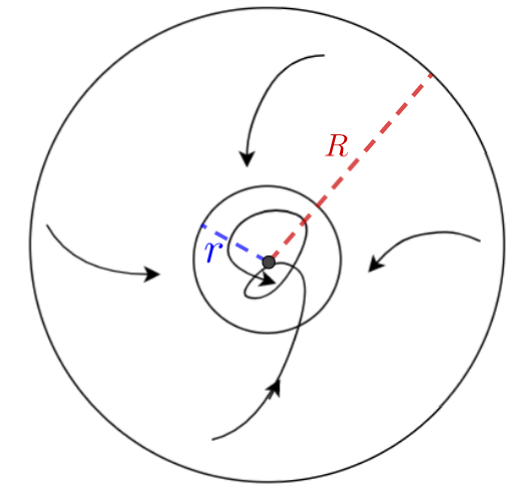
Figure 1: Attracting and invariant balls for a subset of $N-K$ oscillators

Remark 2

We make a few remarks about this theorem. Firstly, we can actually derive analytical expressions for the sizes of the invariant and attracting balls, which are $r=\frac{2K\gamma(N-K)^{1/2}}{N|\lambda_{2}|}$ and $R=\frac{N|\lambda_{2}|}{(N-K)\gamma}$. Here, $\lambda_{2}$ is the second largest eigenvalue of the Jacobian matrix of Equation (1) at $\theta^{*}$. Note that $\lambda_{2}$ depends implicitly on $\gamma$, and as $\gamma$ increases we expect $\lambda_{2}$ to become more negative.

Secondly, The integer $K$ represents the number of free or non-phase-locked oscillators. The function $h(K,N)$ is only defined for $K\leq\frac{\sqrt{16N+1}-1}{8}\approx 0.5N^{\frac{1}{2}}$ for $N$ large, so this theorem can only guarantee the existence a subset of mutually phase-locked oscillators with $K\lesssim 0.5N^{\frac{1}{2}}$ oscillators drifting away. The constant can probably be improved but we think it unlikely that the scaling can be improved without substantially changing the approach.

Typically we will have $g(K,N)<\gamma h(K,N)$ in an interval, so there will be a range of integers $K$ for which the inequality is satisfied. In this situation, we would be primarily interested in the smallest such $K$ that satisfies the inequality, as this would represent the largest partially phase-locked cluster. We denote such $K$ as $K^{*}$. In other words $K*$ is the infimum over all $K$ such that the inequality $g(K,N)<\gamma h(K,N)$ holds.

When $K=0$, corresponding to no free oscillators, the condition on $\gamma$ in this theorem reduces to $\gamma_{\text{critical}}(0)=\omega_{max}-\omega_{min}$, which coincides with Theorem 2.3 of Dorfler and BulloDrfler2011 . Thus this theorem can be viewed as a generalization of their result to the case of partial phase-locking.

3 Proof of Theorem 2.5

In this section, we prove our first main result. A brief sketch of the main idea of the proof is as follows: we first prove a standard proposition: If we take the Kuramoto model in a parameter regime where there is a stable fixed point and we add a small perturbation, then there is an attracting ball of small radius around the former fixed point. In particular, any initial conditions which begin near the fixed point remain so for all time. We then use this result to study partial phase-locking by considering subsets of oscillators that could potentially phase locked, and considering the remaining oscillators as a perturbation to these candidates for partial phase-locking.

Definition 3.1

We say $\theta^{*}$ is a stable phase-locked solution of Equation (1) with frequencies $\bm{\omega}=(\omega_{1},\omega_{2},...,\omega_{N})^{T}$ if it satisfies (1)

$$\omega_{i}=\frac{\gamma}{N}\sum_{j}\sin(\theta_{i}^{*}-\theta_{j}^{*})$$ (8)

and $J$, the Jacobian matrix at $\theta^{*}$, i.e,

$$J_{ij}(\theta^{*})=\begin{cases}\frac{\gamma}{N}\cos(\theta_{i}^{*}-\theta_{j}^{*}),&i\not=j,\\ -\frac{\gamma}{N}\sum_{k\not=i}\cos(\theta_{i}^{*}-\theta_{k}^{*}),&i=j\end{cases}$$

is negative semi-definite with a one dimensional kernel.

Proposition 3.2

Suppose $\theta^{*}$ is a stable phase-locked solution. Consider the following perturbed Kuramoto model with perturbation $\epsilon f_{i}$:

$$\dot{\theta_{i}}=\omega_{i}-\frac{\gamma}{N}\sum_{j}\sin(\theta_{i}-\theta_{j})+\epsilon f_{i}(\theta,t),\qquad i=1,2,...N,$$ (9)

where $\epsilon$ is a small constant and $f_{i}^{\prime}s$ are functions bounded by a constant $C$, i.e., $\max\limits_{\theta,t,i}|f_{i}(\theta,t)|\leq C$. Let

$$\left\{\begin{array}[]{c}r(\epsilon)=2\epsilon CN^{1/2}/|\lambda_{2}|\\ R=|\lambda_{2}|/\gamma,\\ \end{array}\right.$$ (10)

where $\lambda_{2}<0$ is the second largest eigenvalue of the Jacobian matrix of (1) at $\theta^{*}$. Then for $\epsilon<|\lambda_{2}|^{2}/(2CN^{1/2}\gamma)$, the following statements hold:
(1) The ball $||\theta(t)-\theta^{*}||_{N}<r(\epsilon)$ is invariant in forward time.
(2) Every solution with $||\theta(0)-\theta^{*}||_{N}<R$ asymptotically converges to the above invariant ball with radius $r(\epsilon)$.

Proof

We will make a standard Lyapunov function calculation: the proof is sketched here, with details relegated to the Appendix. We will represent $\theta$ as $\theta=\theta^{*}+\tilde{\theta}$. Note that by rotational invariance we can assume $\tilde{\theta}$ is mean zero. Also note that the norm $\|\cdot\|_{\Omega}^{2}$ is equivalent to the standard Euclidean norm $\|\cdot\|^{2}$ on the subspace of mean zero functions: if $\tilde{\theta}$ has mean zero and $\hat{\bm{1}}$ is the vector of all ones then $\|\tilde{\theta}+\alpha\hat{\bm{1}}\|_{\Omega}^{2}=\|\tilde{\theta}\|_{\Omega}^{2}=\sum\tilde{\theta}_{i}^{2}.$

First note that we have an upper bound on $\frac{d}{dt}{||\tilde{\theta}||^{2}}$ of the following form:

$$\frac{d}{dt}{||\tilde{\theta}||^{2}}\leq 2\lambda_{2}||\tilde{\theta}||^{2}+\gamma||\tilde{\theta}||^{3}+2\epsilon CN^{1/2}||\tilde{\theta}||.$$

To make $\frac{d}{dt}{||\tilde{\theta}||^{2}}$ negative, it suffices to require

$$\left\{\begin{array}[]{c}2\epsilon CN^{1/2}||\tilde{\theta}||<|\lambda_{2}|||\tilde{\theta}||^{2}\\ \gamma||\tilde{\theta}||^{3}<|\lambda_{2}|||\tilde{\theta}||^{2},\\ \end{array}\right.$$ (11)

which is equivalent to

$$\frac{2\epsilon CN^{1/2}}{|\lambda_{2}|}<||\tilde{\theta}||<\frac{|\lambda_{2}|}{\gamma}.$$ (12)

Let $r(\epsilon)=2\epsilon CN^{1/2}/|\lambda_{2}|$ and $R=|\lambda_{2}|/\gamma$, then by Gronwall’s inequalityKhalil1993 , the semi-norm of $\tilde{\theta}$ is exponentially decreasing when $\tilde{\theta}$ is in the annulus of radii $r(\epsilon)$ and $R$, and then stays in the ball of radius $r(\epsilon)$ forever. So statements (1) and (2) are proved.

Now, we use Proposition 3.2 to prove Theorem 2.5.

Proof

For any integer $0\leq K<N$, consider $N-K$ oscillators in the Kuramoto model (1). By changing the order of labels, we can, without loss of generality, focus on the first $N-K$ oscillators and study the conditions under which they will stably phase-lock. The evolution can be written as follows

$$\dot{\theta}_{i} =\omega_{i}-\frac{\gamma}{N}\sum_{i=1}^{N}\sin(\theta_{i}-\theta_{j})$$ (13)

$$=\omega_{i}-\frac{\gamma}{N}\sum_{j=1}^{N-K}\sin(\theta_{i}-\theta_{j})-\frac{\gamma}{N}\sum_{j=N-K+1}^{N}\sin(\theta_{i}-\theta_{j})$$ (14)

$$=\omega_{i}-\frac{\tilde{\gamma}}{N-K}\sum_{j=1}^{N-K}\sin(\theta_{i}-\theta_{j})+\epsilon f_{i}$$ (15)

where $\tilde{\gamma}=\gamma\frac{N-K}{N}$ is a modified coupling strength on the first $N-K$ oscillators and $\epsilon f_{i}$ represents the effect of the remaining $K$ oscillators. Then we have $\epsilon=\frac{\gamma}{N}$, $f_{i}=\sum_{j=N-K+1}^{N}\sin(\theta_{j}-\theta_{i})\leq K$. The strategy is to treat the effect of the remaining $K$ oscillators as a perturbation and then apply Proposition (3.2).

We first consider the unperturbed problem

$$\dot{\theta_{i}}=\omega_{i}-\frac{\tilde{\gamma}}{N-K}\sum_{j=1}^{N-K}\sin(\theta_{i}-\theta_{j}),\qquad i=1,2,...,N-K.$$ (16)

Define

$$\gamma_{0}=\max_{i,j=1}^{N-K}|\omega_{i}-\omega_{j}|.$$

By Theorem 2.3 if the spread in frequencies satisfies

$$\gamma_{0}<\tilde{\gamma}=\frac{\gamma(N-K)}{N},$$ (17)

then Equation (16) phase-locks; the set $\bar{\triangle}(\alpha)$ is positively invariant for every $\alpha\in[\alpha_{min},\alpha_{max}]$, and each trajectory starting in $\triangle(\alpha_{max})$ approaches asymptotically $\bar{\triangle}(\alpha_{min})$, where $\alpha_{min}\in[0,\pi/2)$, $\alpha_{max}\in(\pi/2,\pi]$ and $\sin(\alpha_{min})=\sin(\alpha_{max})=\frac{\gamma_{0}}{\tilde{\gamma}}$. From these, it is clear to see that under a rotating frame with frequency $\omega_{avg}$, Equation (16) has a fixed point $\theta^{*}$ such that $\theta^{*}\in\bar{\triangle}(\alpha_{min})$.

Suppose $L$ is the Jacobian matrix of (16) at the fixed point $\theta^{*}$, i.e,

$$L_{ij}=\begin{cases}\frac{\tilde{\gamma}}{N-K}\cos(\theta_{i}^{*}-\theta_{j}^{*}),&i\not=j,\\ -\frac{\tilde{\gamma}}{N-K}\sum_{k}\cos(\theta_{i}^{*}-\theta_{k}^{*}),&i=j.\end{cases}$$

Since $\theta^{*}\in\bar{\triangle}(\alpha_{min})$ and $\alpha_{min}\in[0,\frac{\pi}{2})$, we have $\cos(\theta^{*}_{i}-\theta^{*}_{j})>0$ and $L$ is a negative semidefinite Laplacian matrix with eigenvalues $\lambda_{1}=0>\lambda_{2}\geq\lambda_{3}\geq...\geq\lambda_{N-K}$, so the solution is stably phase-locked.

We next consider the effects of the perturbation terms $\epsilon f_{i}$ where $\epsilon=\frac{\gamma}{N}$, $f_{i}=\sum_{j=N-K+1}^{N}\sin(\theta_{j}-\theta_{i})\leq K$. Proposition 3.2 guarantees the existence of an invariant ball for the first $N-K$ oscillators when

$$\epsilon=\frac{\gamma}{N}<\frac{|\lambda_{2}|^{2}}{2K(N-K)^{1/2}\tilde{\gamma}},$$ (18)

or equivalently, when

$$\gamma<\sqrt{\frac{1}{2K(N-K)^{3/2}}}\cdot N|\lambda_{2}|.$$ (19)

The eigenvalue $\lambda_{2}$ depends implicitly on $\gamma$ so we need a lower bound on the magnitude of $\lambda_{2}$ in order to close the argument and guarantee that (19) can be satisfied. Since the kernel of $L$ is spanned by $(1,1,1,\ldots,1)$ we can consider the operator $-L$ acting on the space of mean-zero vectors. For any $x$ with $\sum\limits_{i}x_{i}=0$, we have, on the one hand,

$$x^{T}(-L)x =\frac{\gamma}{N}\sum\limits_{i,j}\cos(\theta_{i}^{*}-\theta_{j}^{*})x_{i}^{2}-\frac{\gamma}{N}\sum\limits_{i,j}\cos(\theta_{i}^{*}-\theta_{j}^{*})x_{i}x_{j}$$

$$=\frac{\gamma}{2N}\sum\limits_{i,j}\cos(\theta_{i}^{*}-\theta_{j}^{*})(x_{i}-x_{j})^{2}$$

$$\geq\frac{\gamma}{2N}\min_{i,j}\cos(\theta_{i}^{*}-\theta_{j}^{*})\sum\limits_{i,j}(x_{i}-x_{j})^{2}$$

$$=\frac{\gamma}{N}\min_{i,j}\cos(\theta_{i}^{*}-\theta_{j}^{*})\left((N-K)\sum\limits_{i}x_{i}^{2}-\sum\limits_{i,j}x_{i}x_{j}\right)$$

$$=\frac{\gamma(N-K)}{N}\min_{i,j}\cos(\theta_{i}^{*}-\theta_{j}^{*})\|x\|^{2}$$

$$\geq\frac{\gamma(N-K)}{N}\sqrt{1-\frac{\gamma_{0}^{2}}{\tilde{\gamma}^{2}}}\|x\|^{2}.$$

On the other hand,

$$x^{T}(-L)x\leq\frac{\gamma}{2N}\sum_{i,j}(x_{i}-x_{j})^{2}=\frac{\gamma(N-K)}{N}\|x\|^{2}.$$

Therefore we have the inequality

$$\frac{\gamma(N-K)}{N}\sqrt{1-\frac{\gamma_{0}^{2}}{\tilde{\gamma}^{2}}}\leq|\lambda_{2}|\leq\frac{\gamma(N-K)}{N}.$$ (20)

Combining Equations (19) and (20), we can conclude that an invariant ball for the first $N-K$ oscillators with radius $R=\frac{|\lambda_{2}|N}{\gamma(N-K)}$ exists when

$$\gamma_{0}=\max_{i,j=1}^{N-K}|\omega_{i}-\omega_{j}|<\tilde{\gamma}\sqrt{1-\frac{2K}{(N-K)^{1/2}}}.$$ (21)

Therefore, we have proven the first part of Theorem 2.5. In fact, since the above argument holds regardless of the subset of oscillators we choose, we can go through every subset holding $N-K$ elements and target the one with the smallest $K$ such that (21) holds. So we derive a sufficient condition: $g(K,N)\leq\gamma h(K,N)$, where functions $g$ and $h$ are respectively defined in (6) and (7). The existence of an invariant ball of $N-K^{*}$ oscillators where

$$K^{*}:=\min\limits_{K}\{K\in\mathbb{N}:g(K,N)\leq\gamma h(K,N)\}$$ (22)

is guaranteed.

Similarly as Proposition 3.2, it can be concluded that if $||\theta(0)-\theta^{*}||_{S}<R$, then all the oscillators in $S$ asymptotically converges to the invariant ball $||\theta(t)-\theta^{*}||_{S}<r$, where $r=\frac{2\gamma K(N-K)^{1/2}}{N|\lambda_{2}|}$. Therefore, we have a proof for the second part of Theorem 2.5.

4 Numerical Examples

In this section we present several numerical experiments on the Kuramoto model (1) to illustrate our first theorem. In the first two experiments all of the oscillator frequencies are chosen to be i.i.d. Gaussian random variables with small variance except for one or two whose natural frequency is chosen to be large compared with the other oscillators. In the last experiment we consider a case where all oscillators have independent Cauchy distributed natural frequencies.

Example 1 (One free oscillator)

The first experiment depicts a case with $N=20$ oscillators with coupling strength $\gamma=1$. The frequencies $\omega_{1},\omega_{2},...,\omega_{19}$ are chosen to be normal random variables with mean 0 and variance $\frac{\gamma}{N}$, and the frequency $\omega_{20}$ is chosen to be $\gamma+0.1$. One can easily check from the definition that $K^{*}=1$, meaning there exists at most one free oscillator. The cluster of nineteen phase-locked oscillators eventually moves at a common angular frequency $\bar{\omega}$. We use the change of variables $\tilde{\theta}_{i}(t)=\theta_{i}(t)-\bar{\omega}t$ for $i=1,2,...,N$ to work in a frame of reference corotating with the phase-locked cluster. With a slight abuse of notation, we rewrite $\tilde{\theta}$ as $\theta$. The left graph in Figure 2 exhibits the evolution of the phases $\theta_{i}$’s on the real line with respect to time $t$ under the rotation frame; the right graph represents the phase trajectories on the torus. It can be seen that, as expected, there exists a phase-locked cluster of 19 oscillators depicted by the blue curves, and a single free oscillator whose trajectory is depicted by the red curve.

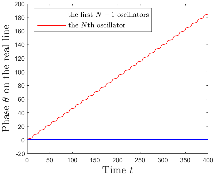
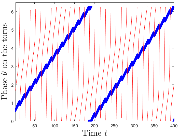
Figure 2: A cluster of 19 phase-locked oscillators and 1 free oscillator.

Figure 3 represents the same experiment from Figure 2, but we have moved to a frame that is co-rotating with the phase-locked cluster and rescaled the graph to more clearly represent the dynamics of the cluster. One can clearly see that after an initial transient the phase-locked cluster settles down to something that appears to be periodic. It is clear that there is a periodic disturbance of the cluster when the free oscillator passes through, although this is not sufficient to break up the cluster. To make this a little more precise, we first computed the frequency of the free oscillator via $\omega_{\text{eff}}=\frac{\theta(T)-\theta(T/2)}{T/2}$ where $T=1000$ is the total running time. This calculation gave $\omega_{\text{eff}}=0.4483$. Next we took the Fourier transform of the trajectory of one of the oscillators in the locked cluster, excluding the initial transient region. The results are depicted in Figure 3, which shows the one-sided spectral power density for a single trajectory. One can see that the trajectories are effectively periodic – the spectrum has peaks at integer multiples of fundamental frequency $\xi\approx.0714$, and that $\omega_{\text{eff}}\approx 2\pi\xi$, as expected.

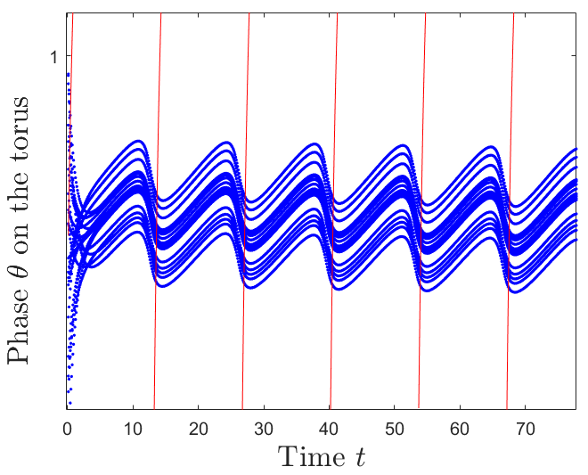
Figure 3: Phase trajectories on the torus under a rotated frame

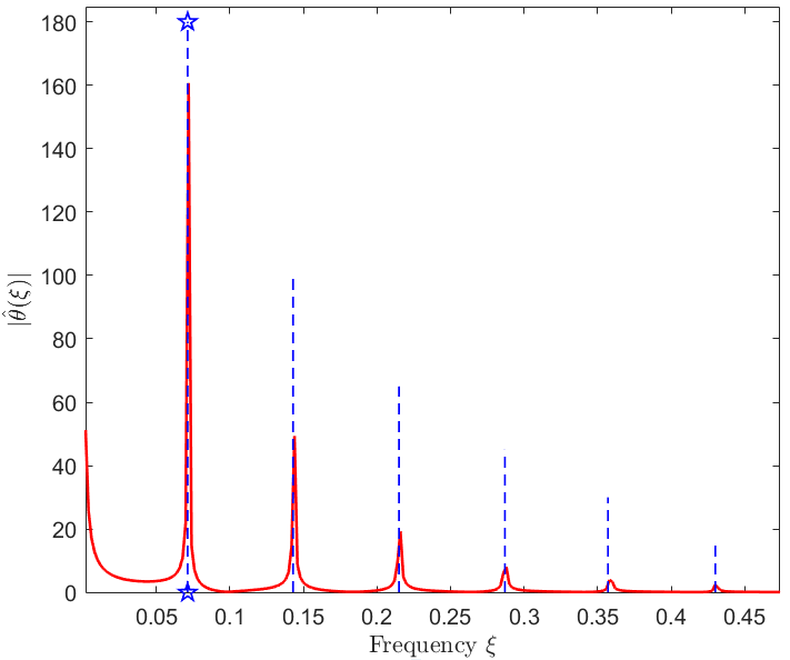
Figure 4: Single-sided amplitude spectrum of a phase-locked trajectory

Example 2 (Two free oscillators)

In this example we still consider a system of $N=20$ oscillators with coupling strength $\gamma=1$, but instead choose the frequencies of two of the oscillators to guarantee that they do not phase-lock to the rest. More precisely the frequencies $\omega_{1},\omega_{2},...,\omega_{18}$ are chosen to be Gaussian random variables with mean 0 and variance $\frac{\gamma}{N}$, and the two free oscillators are chosen to have frequencies $\omega_{19}=\gamma+0.1$ and $\omega_{20}=1.5\gamma+0.01$. As expected $K^{*}=2$, and as before we work in the coordinate system that rotates with the mean frequency of the cluster of $18$ oscillators. The results of a numerical simulation are depicted in Figure 5. As in the first experiment we see a stable cluster of eighteen oscillators with quasi-periodic disturbances as the two free oscillators pass through the cluster.

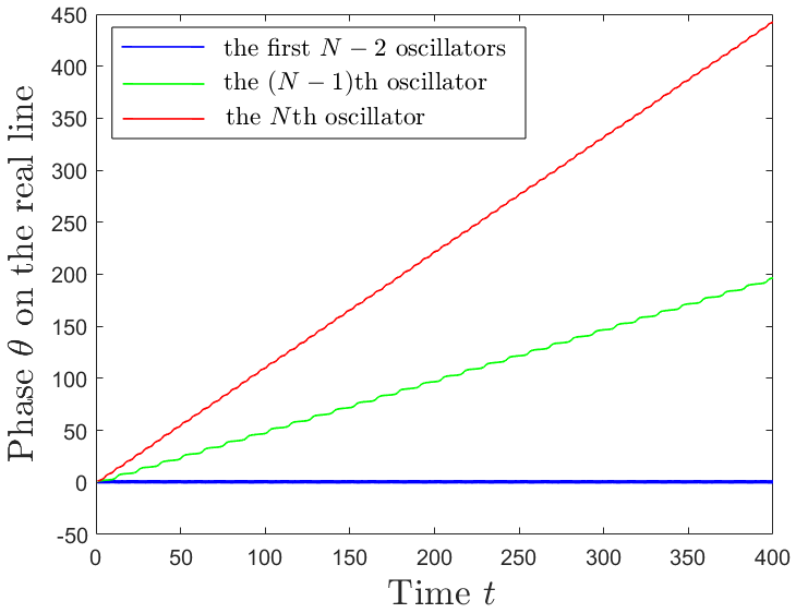
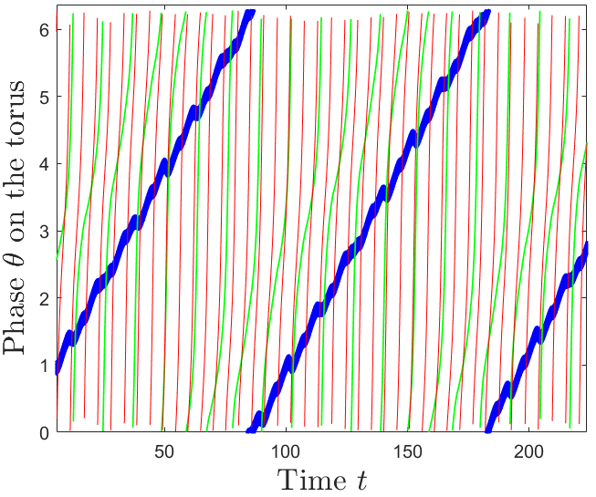
Figure 5: A cluster of 18 phase-locked oscillators and 2 free oscillators.

The left graph in Figure 5 shows the phases of the oscillators in the cluster, which appear to be quasi-periodic. The effect of these two oscillators on the phase-locked ones can be seen from the right graph in Figure 5. Enlarging a portion of this graph and redrawing the trajectories in the co-rotating frame gives Figure 6.

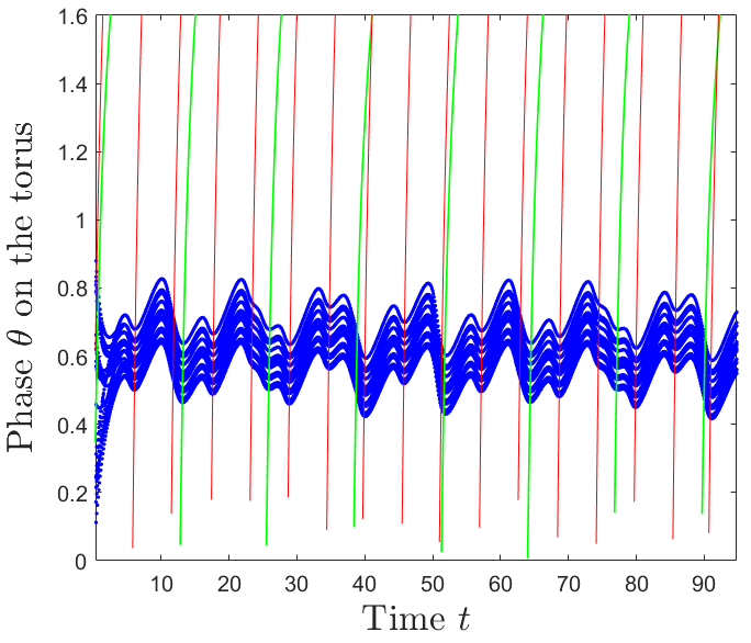
Figure 6: Phase trajectories on the torus under a rotated frame

In a similar manner to the first experiment we expect a relation between the fundamental frequencies of the phase trajectory of a phase-locked oscillator $\xi$ and the angular frequencies of the free oscillator $\tilde{\omega}$: $\tilde{\omega}=2\pi\xi$, Once again we compute the Fourier transform of one of the trajectories in the phase-locked cluster and obtain Figure 7.

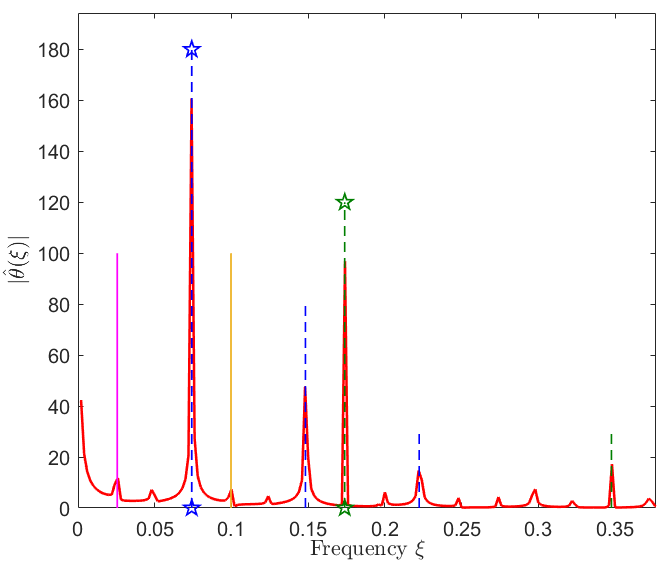
Figure 7: Single-sided amplitude spectrum of a locked phase trajectory

As in the previous experiment we also computed the effective frequencies by $\omega_{\text{eff};19}=\frac{\theta_{19}(T)-\theta_{19}(T/2)}{T/2}$, and found $\omega_{\text{eff};19}\approx 0.4656$ and $\omega_{\text{eff};20}\approx 1.0920$. This agrees well with what we found by computing the Fourier transform of one of the trajectories of an oscillator in the phase-locked cluster. The fundamental frequencies, as seen in Figure 7, are $\xi_{19}=0.0741\approx\omega_{\text{eff};19}/2\pi$ and $\xi_{20}=0.1738\approx\omega_{\text{eff};20}/2\pi$, associated with the two highest peaks denoted by the dashed lines with the star markers, in agreement with the direct numerical measurement. Since the two free oscillators have incommensurate frequencies we would expect to see many smaller peaks associated with various linear combinations of the fundamental frequencies. We have marked the integer multiples of $\xi_{19}$ with blue lines, and multiples of $\xi_{20}$ with green, as well as a couple of other peaks corresponding to other linear combinations. For instance, the pink line denotes a frequency of $\xi_{20}-2\xi_{19}$ and the yellow line a frequency $\xi_{20}-\xi_{19}$. We will not label all of the frequency peaks but all of them correspond to small integer combinations $j\xi_{19}+k\xi_{20}$ with $|j|,|k|\leq 3$.

Remark 3

In the previous two experiments, with one and two free oscillators, the solutions appeared to be periodic and quasi-periodic respectively. It is worth noting that it would probably be quite difficult to prove the existence of a periodic or quasi-periodic solution. Even if one were able to do so a linear stability analysis of the solution would likely be highly non-trivial. In the case of a periodic solution the stability analysis would involve a Floquet problem; these types of problems are difficult to solve in any but the simplest of cases. The spectrum of quasi-periodic operators is even more difficult to understand: in the case of a quasi-periodic Schrödinger operator the spectrum typically lies on a Cantor setJS1994 , rather than simple bands and gaps as in the periodic case. However by showing the existence of a small exponentially attracting ball we can answer the same physical question in a much easier way.

Example 3 (Cauchy distributed oscillators)

The first two numerical experiments were instructive but obviously somewhat contrived in that we picked one or two of the oscillators frequencies by hand to ensure that we had some free oscillators.

In this experiment we take $N=500$ oscillators with coupling strength $\gamma=5$. The frequencies $\omega_{1},\omega_{2},...,\omega_{500}$ were chosen to be standard Cauchy random variables with constant scale $0.01$, i.e., $\omega_{i}\sim 0.01\cdot Cauchy(0,1)$. Of course Cauchy random variables have very broad tails, so we expect large outliers to be relatively common (as compared with, say, a Gaussian distribution). In the experiment depicted here, $\omega_{\max}-\omega_{\min}=7.2161>\gamma=5$, so the necessary condition for full phase-locking is not satisfied. However, partial phase-locking is guaranteed if there exists some integer $K$ such that $g(K)<h(K)$.

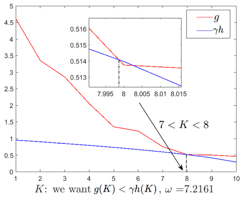
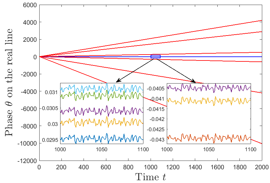
Figure 8: Partially phase-locked oscillators with Cauchy distributed frequencies.

The left graph in Figure 8 shows the graphs of functions $g(K,N)$ (computed directly from the random frequency vector $(\omega_{1},\omega_{2},\ldots,\omega_{500})$) and $\gamma h(K,N)$ with respect to $K$. There is a very small region in which the inequality $g(K)<\gamma h(K)$ holds, from about $7.998$ to about $8.003$. This guarantees the existence of a phase-locked cluster of at least $N-8=492$ oscillators. The theorem does not really say much about the basin of attraction, except to guarantee that it has radius at least $O(1).$ The right graph in Figure 8 shows the evolution of the oscillator phases $\theta_{i}$ with respect to time $t$. In practice we see that the size of the phase-locked cluster is somewhat larger than the minimum guaranteed by the theorem: there are actually 494 phase-locked oscillators and 6 free oscillators. The red curves represent the trajectories of 494 phase-locked oscillators while the blue curves represent 6 free oscillators.

5 Almost sure Entrainment

Our goal in this section is to understand the probability of partial entrainment in the Kuramoto model with randomly distributed frequencies, particularly in the large $N$ limit. The results in the previous section used a relatively strong definition of partial phase-locking, in that we required a subset of oscillators to remain close to an equilibrium configuration. This resulted in fairly strong control on $\|\theta-\theta^{*}\|_{S}$; however while it allowed a large number of non-phase-locked oscillators the percentage as a fraction of the total number had to remain small. In considering the limit $N\rightarrow\infty$ one would really like to allow the possibility that a fixed percentage of the oscillators, possibly small but independent of $N$, would fail to phase-lock. To this end we utilize a very pretty result of De Smet and Aeyels DeSmet2007 that guarantees that a subset of oscillators remains close to one another, while not necessarily being close to any fixed configuration: partial entrainment.

Theorem 5.1 (Aeyels-DeSmet)

For the finite $N$ Kuramoto model (1), if

$$\min\limits_{S\subset\Omega,|S|=N-K}\max\limits_{i,j\in S}|\omega_{i}-\omega_{j}|<\gamma\sqrt{\frac{N}{N-K}}\left(\frac{2N-4K}{3N}\right)^{\frac{3}{2}},$$ (23)

then there exists a subset $S\subset\{1,...,N\}$ with $|S|=N-K$ such that there is an invariant region:

$$\exists C_{S}>0\ s.t.\ |\theta_{i}(t)-\theta_{j}(t)|<C_{S},\ \forall t\geq 0,\ \forall i,j\in S,$$

where $C_{s}=2\arcsin{\sqrt{\frac{N-2K}{6(N-K)}}}$, i.e., the Equation (1) achieves partial entrainment for at least $N-K$ oscillators.

Remark 4

The above result is very strong, in the sense that it can in principle establish entrainment when a positive fraction (up to roughly $1/2$) of the oscillators are free. This is what one would expect from experiments, applications, and the original physical arguments of Kuramoto. On the other hand it does not give very much information about the dynamics. While the angles of the entrained subset of oscillators are guaranteed to remain close to one another there can in principle be $O(1)$ changes in the relative positions of the oscillators, and thus the order parameter is not guaranteed to be constant. One expects that, on average, the free oscillators will not contribute to the order parameter (though there is not proof of that) but even defining a “reduced” order parameter based only on the entrained oscillators the most that one can say is that the order parameter is bounded from above and below. We will discuss this further in the conclusions section.

If we denote the right-hand side of inequality (23) as $\tilde{h}(K,N)$ and let $\rho=\frac{K}{N}$ represent the density of unlocked oscillators, then it is clear that in this new variable $\rho$ that

$$g(\rho)=\min\limits_{S\subset\Omega,\frac{|S|}{N}=1-\rho}\max\limits_{i,j\in S}|\omega_{i}-\omega_{j}|,$$ (24)

$$\tilde{h}(\rho)=\sqrt{\frac{1}{1-\rho}}\left(\frac{2-4\rho}{3}\right)^{\frac{3}{2}}.$$ (25)

In terms of $\rho$, the inequality (23) becomes $g(\rho)<\gamma\tilde{h}(\rho)$. Note that the function $\tilde{h}(\rho)$ is only well-defined when $\rho\leq\rho_{max}=\frac{1}{2}$. Now we are ready to state our second main result as follows.

Theorem 5.2

Consider the Kuramoto model (1) where the natural frequencies $\{\omega_{i}\}_{i=1}^{N}$ are chosen independently and identically distributed from a distribution with the following properties

• The distribution has a density $f(\varpi)$ that is symmetric and unimodal with support on the whole line – the density is increasing on ${\mathbb{R}}^{-}$ and decreasing on ${\mathbb{R}}^{+}.$

• The maximum of the density occurs at $\varpi=0$.

Define the function $g_{\infty}(\rho)$ implicitly by

$$\int_{-\frac{g_{\infty}}{2}}^{\frac{g_{\infty}}{2}}f(\varpi)d\varpi=1-\rho,$$ (26)

and the function $\tilde{h}(\rho)$ by

$$\tilde{h}(\rho)=\sqrt{\frac{1}{1-\rho}}\left(\frac{2-4\rho}{3}\right)^{\frac{3}{2}}.$$

Let $\gamma^{*}$ be the smallest value of $\gamma$ such that there exists a solution to

$$g_{\infty}(\rho)=\gamma\tilde{h}(\rho)\qquad\rho\in(0,\frac{1}{2}].$$ (27)

Then $\gamma^{*}$ is a threshold coupling strength for partial entrainment in the following sense: let ${\mathbb{P}}_{N,\gamma}$ denote the probability that the Kuramoto model admits a partially entrained state with $O(N)$ oscillators. Then

$$\lim_{N\rightarrow\infty}{\mathbb{P}}_{N,\gamma}=1\qquad\forall\gamma>\gamma^{*}.$$

Moreover we have bounds on the size of the largest partially entrained cluster: if $N_{\text{cluster}}$ denotes the number of the oscillators belonging to the largest partially entrained cluster then

$$1-\rho_{\text{min}}\leq\frac{N_{\text{cluster}}}{N}\leq\int_{-\gamma}^{\gamma}f(\varpi)d\varpi.$$

Here, $\rho_{\text{min}}$ is defined as the smallest $\rho$-coordinate of the intersection points of $g_{\infty}(\rho)$ and $\gamma\tilde{h}(\rho)$. The inequality holds in the sense that

$$\lim_{N\rightarrow\infty}{\mathbb{P}}(N_{\text{cluster}}\geq(1-\rho_{\text{min}})N-O(N^{\frac{1}{2}+\epsilon}))=1,$$ (28)

$$\lim_{N\rightarrow\infty}{\mathbb{P}}(N_{\text{cluster}}\leq N\int_{-\gamma}^{\gamma}f(\varpi)d\varpi+O(N^{\frac{1}{2}+\epsilon}))=1.$$ (29)

Remark 5

This is, of course, a sufficient condition ($\gamma>\gamma^{*}$) for partial phase-locking and not a necessary one. Of course based on what is known about the continuous Kuramoto model and the physical arguments on the finite $N$ Kuramoto model one expects (and the numerics to be presented later support this) that partial entrainment occurs for much smaller values of $\gamma$ than are required by the theorem.

As far as the hypotheses go, the second condition that the maximum of the density of the distribution occurs at $\omega=0$ can be assumed w.l.o.g. by working in a co-rotating frame. In the first condition the assumption of symmetry is not really required, and was adopted mostly for ease of exposition, but the assumption that the density is monomodal enters into the proof in a more substantial way. This will be discussed later.

By the definition of $g_{\infty}$, it is clear that $g_{\infty}=2F^{-1}(1-\frac{\rho}{2})$. Under the assumptions of symmetry and unimodality it is easy to compute that $g_{\infty}(\rho)$ is a decreasing functions with a positive second derivative. It is also easy to compute that $\tilde{h}(\rho)$ is a decreasing function with a positive second derivative. In fact, if one can show $(g_{\infty}-\tilde{h})(\rho)$ is a convex function when $\rho\leq\frac{1}{2}$, then it follows that these functions can be equal, $g_{\infty}(\rho)=\tilde{h}(\rho)$, at at most two distinct values of $\rho$, implying that in the continuum limit the range of possible entrained cluster sizes is an interval. Plus, as the coupling strength $\gamma$ increases, $\rho_{\text{min}}$ decreases until the first intersection point vanishes, which implies that partial synchronization becomes full synchronization. For instance, when $\omega_{i}$’s follow standard Gaussian distribution, the graph of the functions $g_{\infty}$ and $\gamma\tilde{h}$ is shown below:

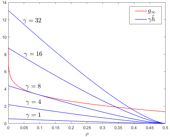
Figure 9: Intersections of $g_{\infty}$ and $\gamma\tilde{h}$ for Gaussian distribution.

To prove Theorem 5.2, we first prove that under the assumptions on the distribution of the $\omega_{i}$, in the limit $N\rightarrow\infty$ the function $g(\rho)$ tends to a deterministic function $g_{\infty}(\rho)$, which is Proposition 30 stated below. Then with Proposition 30 and Theorem 5.1, it is straightforward to derive Theorem 5.2.

Proposition 5.3

Suppose that the natural frequencies $\{\omega_{i}\}_{i=1}^{N}$ are independent, identically distributed random variables satisfying the assumptions in Theorem 5.2, with $f(\varpi)$ the probability density function and $F(\varpi)$ the cumulative distribution function. Then with high probability $g(K,N)$ converges to a deterministic function $g_{\infty}(\rho)$ defined by the Equation 26. More precisely, we have the estimate

$$\lim_{N\rightarrow\infty}{\mathbb{P}}(|g(K,N)-g_{\infty}(\frac{K}{N})|\leq N^{-\frac{1}{2}+\epsilon})=1.$$ (30)

Proof (Sketch of proof)

Define $a=F^{-1}(1-\frac{\rho}{2})$ so that we have $g_{\infty}=2a$ and define $\delta=\frac{1}{2}N^{-\frac{1}{2}+\epsilon}$. First, using the law of large number theorem, one can easily show $g(\rho)\leq 2(a+\delta)$ with probability one. What is less obvious to show is that $g(\rho)\geq 2(a-\delta)$ with probability one where $\delta=\frac{1}{2}N^{-\frac{1}{2}+\epsilon}$ and $\epsilon>0$. In other words, we need to prove

$$\mathbb{P}(A)\to 0\ \text{as}\ N\to\infty,$$ (31)

where $A$ is the event that “there exists an interval with length $L=2(a-\delta)$ containing more than $(1-\rho)N$ points”. Notice that if no intervals of Length $L$ with $\omega_{k}$ at an endpoint contain more than $m$ points then no any other interval does. So we can only focus on $N$ intervals $\{[\omega_{i},\omega_{i}+L]:i=1,2,...,N\}$. Moreover, the interval centered at zero maximizes the probability that a point lies in the interval, i.e., $I=[-L/2,L/2]$ gives the largest $\mathbb{P}(x\in I)$ among all intervals of length $L$. Based on these observations, it is not hard to see

$$\mathbb{P}(A)\leq N\sum\limits_{M=\lceil(1-\rho)N\rceil}^{N}\binom{N}{M}p^{M}(1-p)^{N-M},$$ (32)

where $1-\rho=\int_{-a}^{a}f(x)dx$ and $p=\int_{-L/2}^{L/2}f(x)dx=\int_{-a+\delta}^{a-\delta}f(x)dx$. Using the Stirling approximation, one can prove that the right-hand side of the inequality (32) approaches zero as $N$ approaches infinity. So we are done. This is the main idea of our proof, the full proof can be found in Appendix.

Proposition 30 suggests Equation (28), a probabilistic lower bound on the number of oscillators in a partially entrained cluster. On the other hand, the probabilistic upper bound, given by Equation (29) in Theorem 5.2, is implied by the central limit theorem. We formalize it in the following proposition.

Proposition 5.4

Consider the finite $N$ Kuramoto model (1) where the frequencies $\omega_{i}$ are independent and identically distributed according to a distribution with a density $f(\omega)$ that is symmetric and monomodal, with the unique maximum of $f$ occuring at $\omega=0$. Then the probability that there is any partially entrained cluster containing more than

$$N\int_{-\gamma}^{\gamma}f(\varpi)d\varpi+O(N^{\frac{1}{2}+\epsilon})$$

tends to zero as $N\rightarrow\infty$.

Proof (Sketch of proof)

The proof of this is straightforward and similar to previous arguments, so we just give the broad strokes. The basic observation is that from the usual ${\ell}_{1}/{\ell}_{\infty}$ estimate we have that a subset of oscillators cannot be partially entrained if

$$\omega_{max}-\omega_{min}\geq 2\gamma.$$

By the usual central limit theorem arguments the number of $\omega_{i}$ lying in an interval $I$ is, for $N$ large, approximately $\int_{I}f(\omega)$. We would like to guarantee that (with high probability) there is no interval of length $I$ containing substantially more frequencies than that. Since $f$ is symmetric and monomodal the interval of length $|I|=2\gamma$ which maximizes $\int_{I}f(\omega)$ is the symmetric one, so the largest cluster will, with high probability, have no more than $\int_{-\gamma}^{\gamma}f(\omega)d\omega$.

Remark 6

It is worth comparing this with the minimum cluster size guaranteed by Theorem 5.2. The condition $g_{\infty}(\rho)\leq\gamma\tilde{h}(\rho)$ defines the largest guaranteed cluster size $1-\rho^{*}$ as a somewhat complicated implicit function of the coupling strength $\gamma$, but this simplifies greatly in the limit of large coupling strength $\gamma$. In the limit $\gamma\gg 1$ we have that $\rho\ll 1$ and the partial synchronization condition becomes $g_{\infty}(\rho)\leq\gamma\tilde{h}(0)=\gamma(2/3)^{\frac{3}{2}}.$ Thus the theorem guarantees a partially locked cluster of size at least

$$N_{\text{\rm cluster}}\gtrsim\int_{-(\frac{2}{3})^{\frac{3}{2}}\frac{\gamma}{2}}^{(\frac{2}{3})^{\frac{3}{2}}\frac{\gamma}{2}}f(\omega)d\omega$$

for large $\gamma$.

6 Numerical Examples

In this section, we give two examples to support Theorem 5.2. In the first example, we consider oscillators with Gaussian distributed natural frequencies. In the second example, we consider oscillators with Cauchy distributed natural frequencies.

Example 4

For the case of Gaussian distributed natural frequencies $\omega_{i}$ the function $g_{\infty}(\rho)$ is the inverse function to the error function:

$$g_{\infty}(\rho)=2\sqrt{2}\operatorname{erf}^{-1}(1-\rho).$$

Numerical calculations show that in the thermodynamic limit the minimum coupling in order to guarantee the existence of partially entrained states is $\gamma^{*}\approx 8.0027\sigma$, where $\sigma$ is the variance of the Gaussian distribution (it is clear from scaling that the critical coupling strength should be proportional to the variance). For this critical value of $\gamma$ we have $g_{\infty}(\rho)=\gamma^{*}\tilde{h}(\rho)$ at $\rho\approx.0901$. Thus for a Gaussian distribution of frequencies the theorem guarantees the existence of a partially synchronized cluster containing all but about $9\%$ of the oscillators.

We illustrate Proposition 30, with $N=10000$ oscillators with coupling strength $\gamma=10$ and suppose the natural frequencies follow standard Gaussian distribution $\mathcal{N}(0,1)$. In Figure 10 we plot the function

$$g(\rho)=\min_{S\subset\Omega~{}~{}|S|=(1-\rho)N}\max_{i,j\in S}|\omega_{i}-\omega_{j}|,$$

the function $g_{\infty}(\rho)$ and the curves $g_{\infty}(\rho)\pm\frac{1}{\sqrt{N}}$. One can see that, as expected, the actual curve typically lies within $O(N^{-\frac{1}{2}})$ of the limiting curve.

We note at this point that it is difficult to see a sharp distinction between partial phase-locking regime and the full phase-locking regime for Gaussian distributed random variables in numerical simulations. The reason for this is clear: partial phase-locking takes place in the mean-field scaling

$$\frac{d\theta_{i}}{dt}=\omega_{i}+\frac{\gamma}{N}\sum\sin(\theta_{j}-\theta_{i})$$

while for Gaussian distributed frequencies full phase-locking takes place in the slightly more strongly coupled scaling

$$\frac{d\theta_{i}}{dt}=\omega_{i}+\frac{\gamma\sqrt{\log{N}}}{N}\sum\sin(\theta_{j}-\theta_{i}).$$

In order to get a clean separation of scales one would like $\sqrt{\log(N)}\gg 1$, which is numerically challenging. As an example choosing $\sqrt{2\log{N}}\geq 8$ would guarantee that (by the results of Bronski, DeVille and Park) that full phase locking does not occur and (by the above) that partial phase-locking does occur. This would require an $N$ in the range $N\gtrsim 10^{14}$, which is not numerically feasible. The partial phase-locking behaviour is much easier to observe for distributions with broader tails. This motivates our next example, that of Cauchy distributed frequencies.

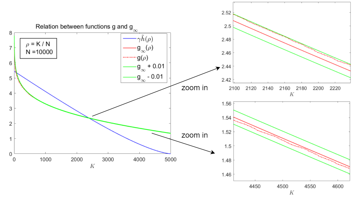
Figure 10: Comparison between functions $g$ and $g_{\infty}$ for Gaussian distribution

Example 5

For the case of Cauchy distributed natural frequencies $\omega_{i}$, their pdf and cdf are as follows:

$$f(\varpi;k,\lambda)=\frac{1}{k\pi(1+(\frac{\varpi-\lambda}{k})^{2})},$$ (33)

$$F(\varpi;k,\lambda)=\frac{1}{\pi}\arctan(\frac{\varpi-\lambda}{k})+\frac{1}{2},$$ (34)

where $k$ is the scale parameter, and $\lambda$ is the location parameter, specifying the location of the peak of the distribution. We consider the case when $\lambda=0$. The function $g_{\infty}(\rho)$ is the inverse function to the cumulative distribution (sometimes called the quantile function):

$$g_{\infty}(\rho)=2\tan(\frac{\pi}{2}(1-\rho)).$$

Numerical calculations show that in the thermodynamic limit the minimum coupling in order to guarantee the existence of partially entrained states is $\gamma^{*}\approx 21.4950k$, where $k$ is the Cauchy scale parameter. It is clear from scaling that the critical coupling strength should be proportional to the scale parameter $k$. For this critical value of $\gamma$ we have $g_{\infty}(\rho)=\gamma^{*}\tilde{h}(\rho)$ at $\rho\approx.2258$. Thus for a Cauchy distribution of frequencies the theorem guarantees the existence of a partially synchronized cluster containing all but about $22.58\%$ of the oscillators for . $\gamma^{*}\approx 21.4950k.$

As a numerical illustration of Proposition 30, we consider $N=10000$ oscillators with coupling strength $\gamma=50$ and suppose the natural frequencies follow Cauchy distribution with $k=1,\lambda=0$. We have that $|g(\rho)-g_{\infty}(\rho)|=o(N^{-\frac{1}{2}+\epsilon})$. The graphs of $g$ and $g_{\infty}$ are shown in Figure 11, along with the curves $g_{\infty}\pm\frac{1}{\sqrt{N}}=g_{\infty}\pm 0.01$. As is clear from the figure we see the typical central limit type convergence of $g(\rho)$ to $g_{\infty}(\rho)$.

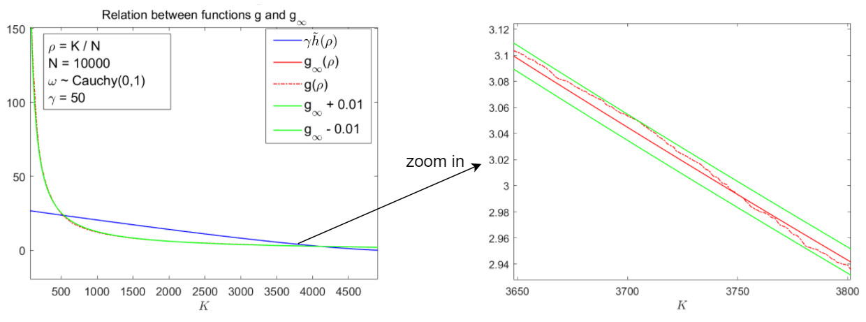
Figure 11: Comparison between functions $g$ and $g_{\infty}$ for Cauchy distribution

Next, we present a simulation to illustrate Theorem 5.2. In this simulation we take the Cauchy scale parameter to be $k=1$ and the location parameter $\lambda=0$. We take $N=500$ oscillators, $\omega_{1}=0$ and $\omega_{i}\sim f(x;1,0)$ for $i=2,...,N$, then direct calculation gives $\gamma^{*}=21.4950$. Our numerical criteria for determining if an oscillator is part of the entrained cluster is as follows. We assume that oscillator number 1, which has zero frequency, is part of any entrained cluster. Define $\Phi_{1i}=\theta_{i}(\frac{T}{2})-\theta_{1}(\frac{T}{2})$, $\Phi_{2i}=\theta_{i}(T)-\theta_{1}(T)$ and $\Psi_{i}=(\Phi_{2i}-\Phi_{1i})\times\frac{2}{T}$. Then we have $\Psi_{i}\to\omega_{i\infty}-\omega_{1\infty}\ \text{as}\ T\to\infty,$ and thus, $\Psi_{i}$ approaches zero if $\theta_{i}$ is locked with $\theta_{1}$. Now, define a relative frequency difference: $d=10^{-5}\times(\max_{i}(\Psi_{i})-\min_{i}(\Psi_{i}))$, where $10^{-5}$ is a tolerance that we choose to classify phase-locked oscillators. If $\Psi_{i}\leq d$, we regard $\theta_{i}$ as the oscillator that locks with $\theta_{1}$. To see the effect of $\gamma$ on the partial entrainment, we vary $\gamma$ from 1 to 25, and for each $\gamma$, use 5 samples of $\omega_{i}$ to solve Equation (1) numerically up to time $T=500$ with a time step $dt=0.1$. Then we compute the average number of oscillators in the largest cluster with frequency difference less than $d$, i.e, $\Psi_{i}\leq d$, over the 5 simulations. The histogram graphs of the amount of oscillators corresponding to $\gamma=5$ and $\gamma=25$ are drawn separately in Figure 12, where the $x$-axis is the frequency difference $\Psi_{i}$ and the $y$-axis is the average number of oscillators satisfying $\Psi_{i}\in(x-\frac{d}{2},x+\frac{d}{2})$. The graphs show, as we expected, the size of the largest cluster of phase-entrained oscillators is larger for $\gamma=25$ than which of $\gamma=5$.

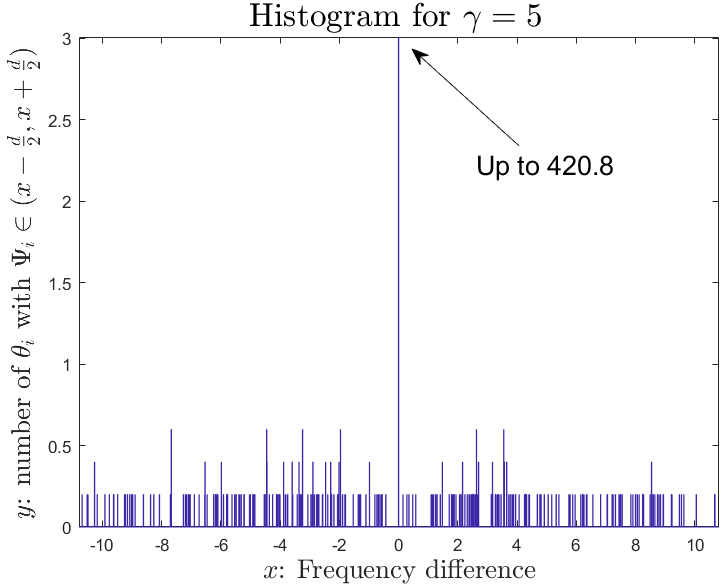
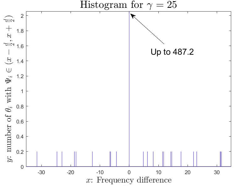
Figure 12: Histogram graphs of average number of entrained oscillators: left: $\gamma=5$; right: $\gamma=25$

In the next experiment we define three percentages $P_{\text{numeric}}$, $P_{\text{lower}}$ and $P_{\text{upper}}$ and make a careful comparison among them as a function of the coupling strength $\gamma$. Firstly let $P_{\text{numeric}}$ denote the average percentage of oscillators in the largest phase-entrained cluster over the 5 simulations. For instance, the realizations in the right graph in Figure 12 give $P_{\text{numeric}}=\frac{487.2}{500}\approx 97\%$ when $\gamma=25$. Secondly, we note the well-known $\ell_{1}-\ell_{\infty}$ estimate: namely that if we have

$$|\omega_{i}-\omega_{j}|>2\gamma\geq\frac{2\gamma}{N}|\sum_{j=1}^{N}\sin(\theta_{j}-\theta_{i})|,$$ (35)

then the $ith$ oscillator and $jth$ oscillator will never synchronize. Thus, by the law of large number, the percentage of oscillators that lock together must be (with high probability) less than $\int_{-\gamma}^{\gamma}f(x;1,0)dx+o(1)$. We let $P_{\text{upper}}$ denote this percentage, i.e., $P_{\text{upper}}=\int_{-\gamma}^{\gamma}f(x;1,0)dx$. Finally, according to Theorem 5.2, we know that as $\gamma>\gamma^{*}=21.4950$, there are at least $n=(1-\rho_{\min})\times N$ oscillators locking together, where $\rho_{\min}$ is defined as the $\rho$-coordinate of the first intersection point of $g_{\infty}$ and $\gamma\tilde{h}$. Let $P_{\text{lower}}$ denote the percentage of oscillators in the largest phase-entrained cluster derived from this theorem, i.e., $P_{\text{lower}}=1-\rho_{\text{min}}$.

Obviously, we have the following inequality

$$P_{\text{lower}}\leq P_{\text{numeric}}\leq P_{\text{upper}}.$$ (36)

As a numerical check of inequality (36), we consider a sequence of values of the coupling strength $\gamma$. For each value of $\gamma$ we plot $P_{\text{numeric}}$, the percentage of oscillators in the largest entrained cluster, as well as $P_{\text{upper}}$ and $P_{\text{lower}}$. Note that when $\gamma<\gamma^{*}=21.4950$, functions $g_{\infty}$ and $\gamma\tilde{h}$ have no intersections, so our theorem cannot guarantee any cluster of phase-entrained oscillators. Therefore, $P_{\text{lower}}=0$ when $\gamma<\gamma^{*}=21.4950$, as seen in Figure 13. It is clear that, at least for the range of $\gamma$ considered the upper bound from the $\ell_{1}-\ell_{\infty}$ estimate and the law of large numbers is actually a very good approximation to the observed number of entrained oscillators.

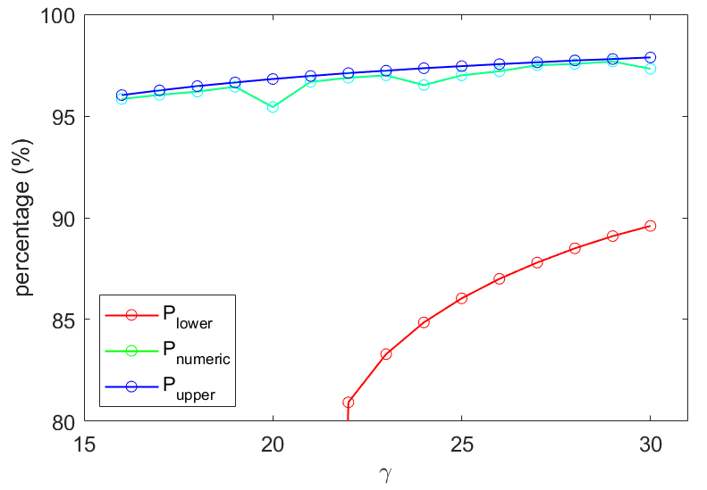
Figure 13: Largest cluster of partial synchronization for Cauchy distribution

It is interesting to consider the asymptotic percentage of entrained oscillators for large coupling strength $\gamma$. Note that as $\gamma$ grows large, $\rho_{\text{min}}$ tends to approach zero, and thus, $\tilde{h}(\rho)$ approaches $(\frac{2}{3})^{\frac{3}{2}}$. From Equation (27), we have

$$g_{\infty}(\rho)\to(\frac{2}{3})^{\frac{3}{2}}\gamma\approx 0.544\gamma\ \text{as}\ \rho\to 0.$$

Using the definition of $g_{\infty}$ as given by (26), it is easy to compute that $\rho_{\text{min}}=2\int_{(\frac{2}{3})^{\frac{3}{2}}\frac{\gamma}{2}}^{\infty}f(x)dx\approx 2\int_{0.272\gamma}^{\infty}f(x)dx$. Thus, when $\gamma$ is large,

$$P_{\text{lower}}\sim 1-2\int_{0.272\gamma}^{\infty}f(x)dx.$$ (37)

Denote the right-hand side as $P_{\text{lower asym}}$, i.e., $P_{\text{lower asym}}=1-2\int_{0.272\gamma}^{\infty}f(x)dx$. Then for the Cauchy distribution, $(1-P_{\text{lower asym}})\sim\frac{1}{\gamma}$, i.e., the percentage of unlocked oscillators is inversely proportional to the coupling strength when the strength is large. On the other hand, for $P_{\text{upper}}$, by its definition, we have for any $\gamma>0$,

$$P_{\text{upper}}=1-2\int_{\gamma}^{\infty}f(x)dx.$$ (38)

The order parameter $r$, defined by

$$r(t)=\mid\frac{1}{N}\sum\limits_{j=1}^{N}e^{i\theta_{j}(t)}\mid,$$ (39)

is a widely used proxy for synchronization. It is worthwhile to plot the evolution of the order parameter as a function of time for some different values of the coupling strength $\gamma$. Specifically we choose $\gamma=\gamma^{*}/2,\gamma^{*},2\gamma^{*}$, where $\gamma^{*}$ is the minimum coupling strength required by the theorem in order to guarantee the existence of a partially entrained state. As one can see from Figure 14 we see the prder parameter $r(t)$ oscillate around a non-zero mean for values of $\gamma$ substantially below the $\gamma^{*}$ required by the theorem.

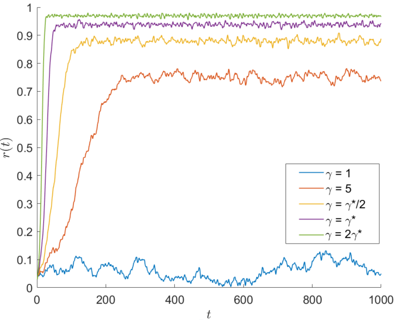
Figure 14: Order parameter $r(t)$ for different coupling strength

7 Conclusions

In this paper, we derived an explicit analytical expression for a sufficient condition on the coupling strength $\gamma$ to achieve partial phase-locking (entrainment) in the classical finite-N Kuramoto model (1) for any arbitrary monomodal distribution of the natural frequencies. We also derived explicit upper and lower bounds on the percentage of entrained oscillators, again as a function of the coupling strength. This result can be veiwed as an extension of the result of F.Dörfler and F.Bullo Drfler2011 on full phase-locking to the case of partial phase locking. The requirement that the distribution of frequencies be monomodal is interesting, in that other authors have identified a change in the nature of the bifurcation when one moves from mono-modal distributions to bimodal or trimodal. In the work of Acebrón, Perales and SpiglerAPS , for instance, the authors identify a change in the nature of the bifurcation, from subcritical to supercritical, as one moves from monomodal to multimodal distributions.

While the scaling of the result is optimal – it holds in the usual mean field scaling whereas, for instance, full phase-locking requires a slightly stronger coupling than the mean field coupling – the constants are almost certainly not optimal and could likely be improved. It is interesting, in fact, that the numerical experiments suggest that the size of the largest entrained cluster is well-predicted by the upper bound given by the law of large numbers. It would be interesting to see if one could derive a lower bound that is closer to the current upper bound.

Appendix A Proof of Proposition 3.2

Proof

Suppose $J$ is the Jacobian matrix of (1) at $\theta^{*}$, $\lambda_{1},\lambda_{2},...,\lambda_{N}$ are $N$ eigenvalues of $J$ and $v_{1},v_{2},...,v_{N}$ are the corresponding eigenvectors. Since $\theta^{*}$ is a stable fixed point, by definition, $\lambda_{N}\leq\lambda_{N-1}\leq...\leq\lambda_{2}<\lambda_{1}=0$. And clearly, $v_{1}=\hat{\textbf{1}}=(1,1,...,1)$. Let $V=Ker(J)=\text{span}\{\hat{\textbf{1}}\}$ and $W=\text{span}\{v_{2},v_{3},...,v_{N}\}$, then $V\oplus W=\mathbb{R}^{N}$.

Now, consider any steady solution of Equation (9) that is close to $\theta^{*}$, i.e., consider $\theta=\theta^{*}+\tilde{\theta}$ where $||\tilde{\theta}||$ is small. Then we have

$$\dot{\theta_{i}}=\dot{\tilde{\theta_{i}}} =\omega_{i}+\frac{\gamma}{N}\sum_{j}\sin(\theta_{j}^{*}-\theta_{i}^{*}+(\tilde{\theta_{j}}-\tilde{\theta_{i}}))+\epsilon f_{i}(\theta,t)$$ (40)

$$=\omega_{i}+\frac{\gamma}{N}(\sum_{j}\sin(\theta_{j}^{*}-\theta_{i}^{*})+\sum_{j}\cos(\theta_{j}^{*}-\theta_{i}^{*})(\tilde{\theta_{j}}-\tilde{\theta_{i}})-\sum_{j}\sin(\xi_{i,j})\frac{(\tilde{\theta_{j}}-\tilde{\theta_{i}})^{2}}{2})$$ (41)

$$\quad+\epsilon f_{i}(\theta,t)\qquad\text{where}\ \xi_{ij}\ \text{is between}\ (\theta_{j}^{*}-\theta_{i}^{*})\ \text{and}\ (\theta_{j}-\theta_{i})\hskip 85.35826pt$$ (42)

$$=\frac{\gamma}{N}\sum_{j}\cos(\theta_{j}^{*}-\theta_{i}^{*})(\tilde{\theta_{j}}-\tilde{\theta_{i}})-\frac{\gamma}{N}\sum_{j}\sin(\xi_{i,j})\frac{(\tilde{\theta_{j}}-\tilde{\theta_{i}})^{2}}{2}+\epsilon f_{i}(\theta,t)$$ (43)

$$=(J\tilde{\theta})_{i}-\frac{\gamma}{N}\sum_{j}\sin(\xi_{i,j})\frac{(\tilde{\theta_{j}}-\tilde{\theta_{i}})^{2}}{2}+\epsilon f_{i}(\theta,t),$$ (44)

where $(J\tilde{\theta})_{i}$ refers to the $i$th row of the matrix $J\tilde{\theta}$.

By our definition of semi-norm (4), $||\theta||^{2}=||\theta||^{2}_{\Omega}=\frac{1}{N}\sum\limits_{1\leq i\leq j\leq N}(\theta_{i}-\theta_{j})^{2}=\frac{1}{N}\theta^{T}M\theta$, where $M=$

$$\left(\begin{array}[]{cccccc}N-1&-1&-1&...&-1\\ -1&N-1&-1&...&-1\\ &&......\\ -1&-1&-1&...&N-1\\ \end{array}\right).$$

Notice that $M$ has an eigenvalue 0 with multiplicity 1 and an eigenvalue $N$ with multiplicity $N-1$, so $M$ is positive semi-definite. By computing the derivative of this semi-norm for $\tilde{\theta}\in W$, we have

$$\frac{d}{dt}\|\tilde{\theta}\|^{2} =\frac{1}{N}\frac{d}{dt}\tilde{\theta}^{T}M\tilde{\theta}=\frac{2}{N}\tilde{\theta}^{T}M\dot{\tilde{\theta}}$$

$$\leq\frac{2}{N}\tilde{\theta}^{T}MJ\tilde{\theta}+\frac{\gamma}{N^{2}}\sum_{i,j}|\sin(\xi_{i,j})[(\tilde{\theta}_{i}-\tilde{\theta}_{j})^{2}\sum_{k}\tilde{\theta}_{i}-\tilde{\theta}_{k})]|+\frac{2}{N}\epsilon\tilde{\theta}^{T}Mf$$

$$\leq\frac{2}{N}\tilde{\theta}^{T}MJ\tilde{\theta}+\frac{\gamma}{N^{2}}\sum_{i,j}[(\tilde{\theta}_{i}-\tilde{\theta}_{j})^{2}\sum_{k}|\tilde{\theta}_{i}-\tilde{\theta}_{k}|]+\frac{2\epsilon}{N}||\tilde{\theta}^{T}M||\cdot||f||$$

$$\leq\lambda_{2}\frac{2}{N}\tilde{\theta}^{T}M\tilde{\theta}+\frac{\gamma}{N^{2}}\sum_{i,j}(\tilde{\theta}_{i}-\tilde{\theta}_{j})^{2}(\sum_{k}(\tilde{\theta}_{i}-\tilde{\theta}_{k})^{2})^{1/2}N^{1/2}+\frac{2\epsilon}{N}(N\tilde{\theta}^{T}M\tilde{\theta})^{1/2}\cdot(N^{1/2}C)$$

$$\leq 2\lambda_{2}\|\tilde{\theta}\|^{2}+\gamma\|\tilde{\theta}\|^{3}+2\epsilon CN^{1/2}\|\tilde{\theta}\|.$$

For $\tilde{\theta}\in V$, $\|\tilde{\theta}\|=0$. In this case, since $M\cdot J$ is negative semi-definite, we still have above inequality. Thus for any small $\tilde{\theta}\in\Re^{N}$, we have

$$\frac{d}{dt}{||\tilde{\theta}||^{2}}\leq 2\lambda_{2}||\tilde{\theta}||^{2}+\gamma||\tilde{\theta}||^{3}+2\epsilon CN^{1/2}||\tilde{\theta}||.$$

To find the basin of attraction, it suffices to find the domain of $||\tilde{\theta}||$ such that

$$2\lambda_{2}||\tilde{\theta}||^{2}+\gamma||\tilde{\theta}||^{3}+2\epsilon CN^{1/2}||\tilde{\theta}||<0,$$ (45)

which will be satisfied if

$$\left\{\begin{array}[]{c}2\epsilon CN^{1/2}||\tilde{\theta}||<c_{1}|\lambda_{2}|||\tilde{\theta}||^{2}\\ \gamma||\tilde{\theta}||^{3}<c_{2}|\lambda_{2}|||\tilde{\theta}||^{2},\\ \end{array}\right.$$ (46)

where $c_{1}>0,c_{2}>0$ and $c_{1}+c_{2}\leq 2$. So we need

$$\frac{2\epsilon CN^{1/2}}{c_{1}|\lambda_{2}|}<||\tilde{\theta}||<\frac{c_{2}|\lambda_{2}|}{\gamma}.$$ (47)

It’s clear to see (47) makes sense only when $\epsilon<\frac{c_{1}c_{2}|\lambda_{2}|^{2}}{2CN^{1/2}\gamma}$. Since $c_{1}c_{1}\leq(\frac{c_{1}+c_{2}}{2})^{2}\leq 1$, the loosest bound on $\epsilon$ is $\frac{|\lambda_{2}|^{2}}{2CN^{1/2}\gamma}$, when $c_{1}=c_{2}=1$.

Let $r(\epsilon)=2\epsilon CN^{1/2}/|\lambda_{2}|$ and $R=|\lambda_{2}|/\gamma$, then by Gronwall’s inequality [20], the semi-norm of $\tilde{\theta}$ is exponentially decreasing when $\tilde{\theta}$ is in the annulus of radii $r(\epsilon)$ and $R$, and then stays in the ball of radius $r(\epsilon)$ forever. So statements (1) and (2) in Proposition 3.2 were proved.

Appendix B Proof of Proposition 30

Proof

The goal is to prove Equation (30):

$$\lim_{N\rightarrow\infty}{\mathbb{P}}(|g(K,N)-g_{\infty}(\frac{K}{N})|\leq N^{-\frac{1}{2}+\epsilon})=1,$$

in other words, we need

$$\lim_{N\rightarrow\infty}{\mathbb{P}}(g\leq g_{\infty}+N^{-\frac{1}{2}+\epsilon})=1,$$ (48)

$$\lim_{N\rightarrow\infty}{\mathbb{P}}(g\geq g_{\infty}-N^{-\frac{1}{2}+\epsilon})=1.$$ (49)

For simplicity, define $a=F^{-1}(1-\frac{\rho}{2})$ so that we have $g_{\infty}=2a$ and define $\delta=\frac{1}{2}N^{-\frac{1}{2}+\epsilon}$, then Equations (48) and (49) can be rewritten as

$$\lim_{N\rightarrow\infty}{\mathbb{P}}(g\leq 2(a+\delta))=1,$$ (50)

$$\lim_{N\rightarrow\infty}{\mathbb{P}}(g\geq 2(a-\delta))=1.$$ (51)

Let’s prove Equation (50) first. In fact, we will show $\mathbb{P}(g\leq 2a)$ tends to one as $N\to\infty$. Define $X_{i}$ =

$$\begin{cases}1,&\text{if}\ \omega_{i}\in[-a,a]\\ 0,&\text{if}\ \omega i\notin[-a,a].\\ \end{cases}$$ (52)

Then $X_{i}^{\prime}s$ are i.i.d random variables since $\omega_{i}^{\prime}s$ are i.i.d random variables. Let $X=X_{1}+X_{2}+...+X_{N}$, then $X$ represents the number of $\omega_{i}$ such that $\omega_{i}\in[-a,a]$. By strong law of large number theorem, $\frac{X}{N}$ converges to ${\mathbb{E}}(X_{i})$ almost surely, i.e., ${\mathbb{P}}(\underset{N\to\infty}{\lim}\frac{X}{N}=\int_{-a}^{a}f(x)dx)=1$. Notice that $\int_{-a}^{a}f(x)dx=1-\rho$, so we have ${\mathbb{P}}(\underset{N\to\infty}{\lim}\frac{X}{N}=1-\rho)=1$. Moreover, we know $g(\rho)\leq 2a$ if $X=(1-\rho)N$ by the definition of the function $g$. Therefore, ${\mathbb{P}}(g(\rho)\leq 2a)=1$ as $N\rightarrow\infty$. Equation (50) has been proved.

The other direction Equation (51) is less trivial to prove. Intuitively, we want to show that with high probability no intervals with length $g_{\infty}-2\delta$ contain more than $(1-\rho)N$ points. To show this, we need to firstly make two important observations. First, notice that if no intervals of Length $L$ with $\omega_{k}$ at an endpoint contain more than $m$ points then no any other interval does. So we can only focus on $N$ intervals $\{[\omega_{i},\omega_{i}+L]:i=1,2,...,N\}$. Second, the interval centered at zero maximizes the probability that a point lies in the interval, i.e., $I=[-L/2,L/2]$ gives the largest $\mathbb{P}(x\in I)$ among all intervals of length $L$. The proof follows from the fact that for $\mu=\int_{a}^{a+L}f(x)dx$, its derivative $\frac{d\mu}{da}=f(a+L)-f(a)$ is zero when $a=-\frac{L}{2}$. As a result, the probability that the interval of length $L$ with $\omega_{k}$ at an endpoint contains more than $m$ points is less than the probability that $[-L/2,L/2]$ contains more than $m$ points. Now, fix $L=2(a-\delta)$ where $\delta$ is defined at the beginning of the proof. Define $A_{k}$ as the event that interval $[\omega_{k},\omega_{k}+L]$ containing more than $(1-\rho)N$ points, $A$ as the event that there exists an interval with length $L$ containing more than $(1-\rho)N$ points, and $B$ as the event that $[-L/2,L/2]$ contains more than $(1-\rho)N$ points. Clearly, our goal is to prove

$$\mathbb{P}(A)\to 0\ \text{as}\ N\to\infty.$$ (53)

Due to the above two observations and the union bound, we have

$$\mathbb{P}(A)=\mathbb{P}(\cup_{k=1}^{N}A_{k})\leq\sum_{k=1}^{N}\mathbb{P}(A_{k})\leq N\cdot\mathbb{P}(B).$$ (54)

Note that

$$\mathbb{P}(B)=N\sum\limits_{M=\lceil(1-\rho)N\rceil}^{N}\binom{N}{M}p^{M}(1-p)^{N-M},$$ (55)

where $1-\rho=\int_{-a}^{a}f(x)dx$ and $p=\int_{-L/2}^{L/2}f(x)dx=\int_{-a+\delta}^{a-\delta}f(x)dx$. we denote the right-hand side of Equation (55) as $R(\rho,p,N)$, then it is sufficient to show

$$R(\rho,p,N)\to 0\ \text{as}\ N\to\infty.$$ (56)

Define $\tau_{N,M}:=\binom{N}{M}p^{M}(1-p)^{N-M}=\frac{N!}{M!(N-M)!}p^{M}(1-p)^{N-M}$. Then

$$\log(\tau_{N,M})=\log(N!)-\log(M!)-\log(N-M)!+M\log(p)+(N-M)\log(1-p).$$

For large $N$, using Stirling’s approximation: $\log(N!)\approx N\log(N)-N+\frac{1}{2}\log(2\pi N)$, we have

$$\log(\tau_{N,M}) \approx N\log(N)-N+\frac{1}{2}\log(2\pi N)-M\log(M)+M-\frac{1}{2}\log(2\pi M)$$

$$\quad-(N-M)\log(N-M)+(N-M)-\frac{1}{2}\log(2\pi(N-M))$$

$$\quad+M\log(p)-(N-M)\log(1-p)$$

$$=N\log(N)-M\log(N)-M\log(\frac{M}{N})-(N-M)\log(N)$$

$$\quad-(N-M)\log(\frac{N-M}{N})+M\log(p)-(N-M)\log(1-p)$$

$$\quad+\frac{1}{2}\log\left(\frac{N}{2\pi M(N-M)}\right)$$

$$=N\left(-\frac{M}{N}\log(\frac{M}{N})-(1-\frac{M}{N})\log(1-\frac{M}{N})+\frac{M}{N}\log(p)+(1-\frac{M}{N})\log(1-p)\right)$$

$$\quad+\frac{1}{2}\log\left(\frac{N}{2\pi M(N-M)}\right)$$

$$=N\left(-x\log(x)-(1-x)\log(1-x)+x\log(p)+(1-x)\log(1-p)\right)$$

$$\quad+\frac{1}{2}\log\left(\frac{N}{2\pi x(1-x)}\right)-\log(N)\quad\text{by setting}\ x=\frac{M}{N}.$$

Let

$$\phi(x):=-x\log(x)-(1-x)\log(1-x)+x\log(p)+(1-x)\log(1-p),$$ (57)

then

$$\phi^{\prime}(x)=\log(\frac{p}{1-p})-\log(\frac{x}{1-x})\ \text{ and}\ \phi^{\prime\prime}(x)=\frac{-1}{x(1-x)}<0.$$ (58)

So $\phi$ reaches the largest when $x=p$. And thus, when $N$ is large, the maximum of $\tau_{N,M}$ occurs when $x=\frac{M}{N}=p$. In the neighborhood of the maximum: $x=p+y$, $\phi(x)\approx\frac{-1}{2p(1-p)}y^{2}$. So we have

$$\log(\tau_{N,M})=\frac{1}{2}\log(\frac{1}{2\pi p(1-p)N})-\frac{N}{2p(1-p)}y^{2}+O(y),$$ (59)

and thus

$$\tau_{N,M}\approx\frac{1}{N}\sqrt{\frac{N}{2\pi p(1-p)}}e^{-\frac{Ny^{2}}{2p(1-p)}+O(y)}.$$ (60)

Recall that $1-\rho=\int_{-a}^{a}f(x)dx$ and $p=\int_{-a+\delta}^{a-\delta}f(x)dx$ where $\delta=N^{-\frac{1}{2}+\epsilon}$, then $(1-\rho)-p\sim N^{-\frac{1}{2}+\epsilon}$. So for $M\geq\lceil(1-\rho)N\rceil$, we have $\frac{M}{N}-p\gtrsim N^{-\frac{1}{2}+\epsilon}$, i.e., $y\gtrsim N^{-\frac{1}{2}+\epsilon}$. On the other hand, $y\leq 1-p<1$. Thus

$$\tau_{N,M}\lesssim\frac{1}{N}\sqrt{\frac{N}{2\pi p(1-p)}}e^{-\frac{N^{2\epsilon}}{2p(1-p)}+O(1)}.$$ (61)

So we have

$$R(\rho,p,N) \leq N\cdot N\cdot\left(\frac{1}{N}\sqrt{\frac{N}{2\pi p(1-p)}}e^{-\frac{N^{2\epsilon}}{2p(1-p)}+O(1)}\right)$$

$$=N\sqrt{\frac{N}{2\pi p(1-p)}}e^{-\frac{N^{2\epsilon}}{2p(1-p)}+O(1)},$$

which implies $R(\rho,p,N)\to 0$ as $N\to\infty$ for any positive $\epsilon$. The proof of Equation (51) is now complete.

With the two equations (50) and (51), we proved Proposition (30).

References

- [1] J. A. Acebrón, A. Perales, and R. Spigler. Bifurcations and global stability of synchronized stationary states in the kuramoto model for oscillator populations. Phys. Rev. E, 64:016218, Jun 2001.
- [2] Juan A. Acebrón, L. L. Bonilla, Conrad J. Pérez Vicente, Félix Ritort, and Renato Spigler. The Kuramoto model: A simple paradigm for synchronization phenomena. Reviews of Modern Physics, 77(1):137–185, apr 2005.
- [3] D. Aeyels and J. A. Rogge. Existence of partial entrainment and stability of phase locking behavior of coupled oscillators. Progress of Theoretical Physics, 112(6):921–942, dec 2004.
- [4] Michael Rosenblum Arkady Pikovsky and Jurgen Kurths. Synchronization: a universal concept in nonlinear sciences, volume 12. Cambridge University Press, New York, 2003.
- [5] Jared C. Bronski, Lee DeVille, and Moon Jip Park. Fully synchronous solutions and the synchronization phase transition for the finite-N Kuramoto model. Chaos: An Interdisciplinary Journal of Nonlinear Science, 22(3):033133, 2012.
- [6] Jared C Bronski and Thomas N Gambill. Uncertainty estimates and bounds for the Kuramoto–Sivashinsky equation. Nonlinearity, 19(9):2023, 2006.
- [7] Eduardo Canale and Pablo Monzo. Almost global synchronization of symmetric Kuramoto coupled oscillators. In Systems Structure and Control. InTech, aug 2008.
- [8] Hayato Chiba, Georgi S. Medvedev, and Matthew S. Mizuhara. Bifurcations in the Kuramoto model on graphs. Chaos: An Interdisciplinary Journal of Nonlinear Science, 28(7):073109, July 2018.
- [9] Nikhil Chopra and Mark W. Spong. On exponential synchronization of Kuramoto oscillators. IEEE Transactions on Automatic Control, 54(2):353–357, feb 2009.
- [10] Pierre Collet, Jean-Pierre Eckmann, Henri Epstein, and Joachim Stubbe. A global attracting set for the Kuramoto–Sivashinsky equation. Communications in mathematical physics, 152:203–214, 1993.
- [11] Helge Dietert. Stability and bifurcation for the Kuramoto model. Journal de Mathématiques Pures et Appliquées, 105(4):451–489, April 2016.
- [12] Florian Dörfler and Francesco Bullo. On the critical coupling for Kuramoto oscillators. SIAM Journal on Applied Dynamical Systems, 10(3):1070–1099, jan 2011.
- [13] G.Bard Ermentrout. Synchronization in a pool of mutually coupled oscillators with random frequencies. Journal of Mathematical Biology, 22(1), jun 1985.
- [14] Bastien Fernandez, David Gérard-Varet, and Giambattista Giacomin. Landau damping in the Kuramoto model. Annales Henri Poincaré, 17(7):1793–1823, December 2015.
- [15] Lorenzo Giacomelli and Felix Otto. New bounds for the Kuramoto–Sivashinsky equation. Communications on Pure and Applied Mathematics: A Journal Issued by the Courant Institute of Mathematical Sciences, 58(3):297–318, 2005.
- [16] Michael Goldman, Marc Josien, and Felix Otto. New bounds for the inhomogenous Burgers and the Kuramoto–Sivashinsky equations. Communications in Partial Differential Equations, 40(12):2237–2265, 2015.
- [17] Charles M. Gray. Synchronous oscillations in neuronal systems: mechanisms and functions. Journal of Computational Neuroscience, 1((1-2)):11–38, 1994.
- [18] Seung-Yeal Ha, Taeyoung Ha, and Jong-Ho Kim. On the complete synchronization of the Kuramoto phase model. Physica D: Nonlinear Phenomena, 239(17):1692–1700, sep 2010.
- [19] S. Jitomirskaya and B. Simon. Operators with singular continuous spectrum: Iii. almost periodic schrödinger operators. Communications in Mathematical Physics, 165(1):201–205, 1994.
- [20] Hassan K. Khalil. Nonlinear Systems. Prentice Hall, Upper Saddle River, New Jersey 07458, 3 edition, 2002.
- [21] Yoshiki Kuramoto. Chemical Oscillations, Waves, and Turbulence. Springer Berlin Heidelberg, 1984.
- [22] Yoshiki Kuramoto. Collective synchronization of pulse-coupled oscillators and excitable units. Physica D: Nonlinear Phenomena, 50(1):15–30, 1991.
- [23] B. Nicolaenko, B. Scheurer, and R. Temam. Some global dynamical properties of the Kuramoto–Sivashinsky equations: Nonlinear stability and attractors. Physica D: Nonlinear Phenomena, 16(2):155 – 183, 1985.
- [24] Filip De Smet and Dirk Aeyels. Partial entrainment in the finite Kuramoto- Sakaguchi model. Physica D: Nonlinear Phenomena, 234(2):81–89, oct 2007.
- [25] Steven H. Strogatz. From Kuramoto to Crawford: exploring the onset of synchronization in populations of coupled oscillators. Physica D: Nonlinear Phenomena, 143(1-4):1–20, sep 2000.
- [26] Steven H. Strogatz and Renato E. Mirollo. Stability of incoherence in a population of coupled oscillators. Journal of Statistical Physics, 63(3-4):613–635, May 1991.
- [27] Steven H. Strogatz, Renato E. Mirollo, and Paul C. Matthews. Coupled nonlinear oscillators below the synchronization threshold: Relaxation by generalized landau damping. Physical Review Letters, 68(18):2730–2733, May 1992.
- [28] Vincent Torre. A theory of synchronization of heart pace-maker cells. Journal of Theoretical Biology, 61(1):55–71, 1976.
- [29] Mark Verwoerd and Oliver Mason. Global phase-locking in finite populations of phase-coupled oscillators. SIAM Journal on Applied Dynamical Systems, 7(1):134–160, jan 2008.
- [30] Mark Verwoerd and Oliver Mason. On computing the critical coupling coefficient for the Kuramoto model on a complete bipartite graph. SIAM Journal on Applied Dynamical Systems, 8(1):417–453, jan 2009.
- [31] Ralf W. Wittenberg. Dissipativity, analyticity and viscous shocks in the (de)stabilized Kuramoto–Sivashinsky equation. Physics Letters A, 300(4):407 – 416, 2002.
- [32] Ralf W Wittenberg. Optimal parameter-dependent bounds for Kuramoto–Sivashinsky-type equations. Discrete & Continuous Dynamical Systems-A, 34(12):5325–5357, 2014.