Improved quark coalescence model for spin alignment and polarization of hadrons

Abstract

We propose an improved quark coalescence model for spin alignment of vector mesons and polarization of baryons by spin density matrix with phase space dependence. The spin density matrix is defined through Wigner functions. Within the model we propose an understanding of spin alignments of vector mesons $\phi$ and $K^{*0}$ (including $\overline{K}^{*0}$) in the static limit: a large positive deviation of $\rho_{00}$ for $\phi$ mesons from 1/3 may come from the electric part of the vector $\phi$ field, while a negative deviation of $\rho_{00}$ for $K^{*0}$ may come from the electric part of vorticity tensor fields. Such a negative contribution to $\rho_{00}$ for $K^{*0}$ mesons, in comparison with the same contribution to $\rho_{00}$ for $\phi$ mesons which is less important, is amplified by a factor of the mass ratio of strange to light quark times the ratio of $\left\langle\mathbf{p}_{b}^{2}\right\rangle$ on the wave function of $K^{*0}$ to $\phi$ ($\mathbf{p}_{b}$ is the relative momentum of two constituent quarks of $K^{*0}$ and $\phi$). These results should be tested by a detailed and comprehensive simulation of vorticity tensor fields and vector meson fields in heavy ion collisions.

I Introduction

The Barnett effect Barnett (1935) and the Einstein-de Haas effect Einstein and de Haas (1915) are two well-known effects in materials to connect rotation and spin polarization which can be converted from one to another. Similar effects also exist in ultra-relativistic heavy-ion collisions (HIC), in which a huge orbital angular momentum (OAM) can be generated in the direction perpendicular to the reaction plane and is transferred to the hot and dense medium in the form of the global polarization of hadrons Liang and Wang (2005a, b); Voloshin (2004); Betz et al. (2007); Becattini et al. (2008); Gao et al. (2008) (see, e.g. Wang (2017); Becattini and Lisa (2020); Gao et al. (2020); Liu and Huang (2020), for recent reviews). In microscopic scenarios the transfer of OAM to spin polarization of hadrons is through the spin-orbit coupling in particle scatterings Liang and Wang (2005a); Gao et al. (2008); Zhang et al. (2019); Weickgenannt et al. (2020), while in macroscopic approaches it is through the spin-vorticity coupling in the fluid Becattini et al. (2013a); Csernai et al. (2013); Becattini et al. (2013b); Becattini et al. (2017); Fang et al. (2016); Pang et al. (2016); Florkowski et al. (2018a, b). The global polarization can be measured through the the polarization of hyperons such as $\Lambda$ (including $\bar{\Lambda}$ hereafter) since they have weak decay channels Liang and Wang (2005a). The STAR collaboration has recently measured a non-vanishing global polarization of $\Lambda$ hyperons in Au+Au collisions at $\sqrt{s_{NN}}=7.7-200$ GeV Adamczyk et al. (2017); Adam et al. (2018).

In principle vector mesons can also be polarized in heavy ion collisions, but the polarization of vector mesons cannot be measured since they mainly decay through strong interaction. Instead, $\rho_{00}$, the 00-element of the vector meson’s spin density matrix, can be meaured through the angular distribution of its decay daughters Liang and Wang (2005b); Yang et al. (2018). If $\rho_{00}\neq 1/3$, the distribution is anisotropic and the spin of the vector meson is aligned to the spin quantization direction. In 2008, the STAR collaboration measured $\rho_{00}$ for the vector meson $\phi(1020)$ in Au+Au collisions at 200 GeV, but the result is consistent to $1/3$, indicating no spin alignment within errors Abelev et al. (2008). Recent preliminary data of STAR for the $\phi$ meson’s $\rho_{00}$ (denoted as $\rho_{00}^{\phi}$ hereafter) at lower energies show a significant positive deviation from $1/3$, which is beyond conventional understanding of the polarization Zhou (2018). In Ref. Sheng et al. (2020), some of us proposed that such a large positive deviation of $\rho_{00}^{\phi}$ from 1/3 may possibly be explained by the $\phi$ field. In such a proposal Sheng et al. (2020), a quark coalescence model is employed which is based on spin density operators in momentum space Yang et al. (2018). As the quark polarization comes mainly from vorticity and vector meson fields which are functions of space-time, the space dependence of the quark polarization in Ref. Sheng et al. (2020) is put in a phenomenological way. The purpose of this paper is to improve the quark coalescence model of Ref. Yang et al. (2018) by defining and using spin density operators in phase space with the help of spin Wigner functions. In such an improved quark coalescence model, the quark polarization as a function of space-time can be treated in a rigorous and systematic way. So one can then naturally describe spin alignments of vector mesons such as $\phi$ and $K^{*0}$ (including $\overline{K}^{*0}$ if not stated explicitly) as functions of space-time. It is expected to implement the improved coalescence model in real time simulations and to provide insights in spin alignments of vector mesons.

The paper is organized as follows. In Sect. II, we formulate the improved coalescence model through the spin density matrix in phase space with coordinate dependence. In Sect. III, we give spin polarization of quarks in phase space from vorticity and vector meson fields. In Sect. IV, we analyze global and local polarization of $\Lambda$ (including $\bar{\Lambda}$ if not stated explicitly) using the improved coalescence model. In Sect. V, using the improved coalescence model we formulate spin alignments of vector mesons $\phi$ and $K^{*0}$. In Sect. VI, we solve the Klein-Gordon equation to give vector meson fields generated by point charge sources. Finally we make a summary of the results.

Notations and conventions. We adopt the sign convention for the metric tensor $g^{\mu\nu}=(1,-1,-1,-1)$. A four-vector is represented by Greek indices, e.g, $x^{\mu}$ or $p^{\mu}$ with $\mu=0,1,2,3$. A three-vector is represented in a boldfaced symbol, e.g., $\mathbf{x}$ or $\mathbf{p}$. The components of a three-vector is represented by the Latin index, but we do not distinguish the superscript and subscript, for example, we do not distinguish $\mathbf{x}^{i}$ and $\mathbf{x}_{i}$ with $i=1,2,3$. We use the shorthand notation $[d^{3}\mathbf{p}]\equiv d^{3}\mathbf{p}/(2\pi)^{3}$.

II Spin density matrix and quark coalescence model in phase space

In Ref. Yang et al. (2018), a quark coalescence model is constructed based on the spin density matrix in momentum representation. In order to describe space-time dependence of spin polarization, we need to formulate an improved coalescence model through the spin density matrix in phase space with coordinate dependence. We work at the formation time $t$ of a hadron, for simplicity of notation, throughout the paper we suppress the time dependence of all quantities unless it is necessary to show it explicitly.

In momentum representation, the spin density operator for single particle states is defined as Yang et al. (2018)

$$\rho=\frac{1}{\Omega}\sum_{s}\int[d^{3}\mathbf{p}]w(s,\mathbf{p})\left|s,\mathbf{p}\right\rangle\left\langle s,\mathbf{p}\right|,$$ (1)

where $w(s,\mathbf{p})$ is the weight function corresponding to the particle state with spin $s$ and momentum $\mathbf{p}$, $\Omega$ is the space volume, and the spin-momentum state $\left|s,\mathbf{p}\right\rangle$ is the direct product of the spin state and the momentum state, $\left|s,\mathbf{p}\right\rangle\equiv\left|s\right\rangle\left|\mathbf{p}\right\rangle$. The weight function is given by

$$w(s,\mathbf{p})=\left\langle s,\mathbf{p}\right|\rho\left|s,\mathbf{p}\right\rangle,$$ (2)

which satisfies the normalization condition $\mathrm{Tr}\rho=1$ equivalent to

$$\sum_{s}\int[d^{3}\mathbf{p}]w(s,\mathbf{p})=1.$$ (3)

The definition and convention of single particle states in non-relativistic quantum mechanics are given in Appendix A.

For the quark and antiquark with spin 1/2, the weight functions have the form

$$w(\mathrm{q}\mid s,\mathbf{p}) = \frac{1}{2}f_{\mathrm{q}}(\mathbf{p})\left[1+sP_{\mathrm{q}}(\mathbf{p})\right],$$

$$w(\bar{\mathrm{q}}\mid s,\mathbf{p}) = \frac{1}{2}f_{\bar{\mathrm{q}}}(\mathbf{p})\left[1+sP_{\bar{\mathrm{q}}}(\mathbf{p})\right],$$ (4)

where $s=\pm$ label two spin states with $s_{z}=\pm 1/2$ in the spin quantization direction $z$, and $f_{\mathrm{q}/\bar{\mathrm{q}}}(\mathbf{p})$ and $P_{\mathrm{q}/\bar{\mathrm{q}}}(\mathbf{p})$ denote the distribution and polarization of the quark/antiquark respectively. Here the quark polarization is normalized to 1 and given by

$$P_{\mathrm{q}}(\mathbf{p})=\frac{w(\mathrm{q}\mid+,\mathbf{p})-w(\mathrm{q}\mid-,\mathbf{p})}{w(\mathrm{q}\mid+,\mathbf{p})+w(\mathrm{q}\mid-,\mathbf{p})}.$$ (5)

The polarization for antiquark $P_{\bar{\mathrm{q}}}(\mathbf{p})$ has the same form as above. We note that generally the weight functions (4) are $2\times 2$ matrices in spin space. Throughout this paper we assume that they are diagonalized in the spin quantization direction.

Now we generalize (1) by introducing the space variable into the density operator as

$$\rho=\sum_{s}\int d^{3}\mathbf{x}\int[d^{3}\mathbf{p}]w(s,\mathbf{x},\mathbf{p})\int[d^{3}\mathbf{q}]e^{-i\mathbf{q}\cdot\mathbf{x}}\left|s,\mathbf{p}+\frac{\mathbf{q}}{2}\right\rangle\left\langle s,\mathbf{p}-\frac{\mathbf{q}}{2}\right|.$$ (6)

We see that the momenta of state bases differ by $\mathbf{q}$ with $\mathbf{x}$ being its conjugate position. The weight function $w(s,\mathbf{x},\mathbf{p})$ is actually the Wigner function which can be obtained by projecting the above density operator onto two states with the same spin and different momenta

$$w(s,\mathbf{x},\mathbf{p})=\int[d^{3}\mathbf{q}]e^{i\mathbf{q}\cdot\mathbf{x}}\left\langle s,\mathbf{p}+\frac{\mathbf{q}}{2}\left|\rho\right|s,\mathbf{p}-\frac{\mathbf{q}}{2}\right\rangle.$$ (7)

By an integration over $\mathbf{x}$ for $w(s,\mathbf{x},\mathbf{p})$ one can recover the weight function (2), therefore the normalization condition for $w(s,\mathbf{x},\mathbf{p})$ reads

$$\sum_{s}\int d^{3}\mathbf{x}\int[d^{3}\mathbf{p}]w(s,\mathbf{x},\mathbf{p})=1.$$ (8)

From above condition one can see that $w(s,\mathbf{x},\mathbf{p})$ is dimensionless. For the quark and antiquark, with new weight functions $w(\mathrm{q}/\bar{\mathrm{q}}\mid s,\mathbf{x},\mathbf{p})$ we have similar formula to Eqs. (4,5) with the distribution $f_{\mathrm{q}/\bar{\mathrm{q}}}(\mathbf{x},\mathbf{p})$ and polarization $P_{\mathrm{q}/\bar{\mathrm{q}}}(\mathbf{x},\mathbf{p})$ as functions in phase space.

II.1 Mesons

To describe the formation of mesons from a quark and an antiquark, we define the spin density operator for a quark-antiquark pair

$$\rho_{\mathrm{q}\bar{\mathrm{q}}} = \sum_{s_{1},s_{2}}\sum_{\mathrm{q}_{1},\bar{\mathrm{q}}_{2}}\int d^{3}\mathbf{x}_{1}d^{3}\mathbf{x}_{2}\int[d^{3}\mathbf{p}_{1}][d^{3}\mathbf{p}_{2}]\int[d^{3}\mathbf{q}_{1}][d^{3}\mathbf{q}_{2}]$$ (9)

$$\times w(\mathrm{q}_{1}|s_{1},\mathbf{x}_{1},\mathbf{p}_{1})w(\bar{\mathrm{q}}_{2}|s_{2},\mathbf{x}_{2},\mathbf{p}_{2})e^{-i\mathbf{q}_{1}\cdot\mathbf{x}_{1}}e^{-i\mathbf{q}_{2}\cdot\mathbf{x}_{2}}$$

$$\times\left|\mathrm{q}_{1},\bar{\mathrm{q}}_{2};s_{1},s_{2};\,\mathbf{p}_{1}+\frac{\mathbf{q}_{1}}{2},\mathbf{p}_{2}+\frac{\mathbf{q}_{2}}{2}\right\rangle$$

$$\times\left\langle\mathrm{q}_{1},\bar{\mathrm{q}}_{2};s_{1},s_{2};\,\mathbf{p}_{1}-\frac{\mathbf{q}_{1}}{2},\mathbf{p}_{2}-\frac{\mathbf{q}_{2}}{2}\right|,$$

where $\mathrm{q}_{1}=$u,d,s and $\bar{\mathrm{q}}_{2}=\bar{\mathrm{u}},\bar{\mathrm{d}},\bar{\mathrm{s}}$ denote the quark and antiquark respectively, the sum over quark and antiquark flavors have been taken, the quark-antiquark state is the direct product of the quark state and the antiquark state

$$\left|\mathrm{q}_{1},\bar{\mathrm{q}}_{2};s_{1},s_{2};\,\mathbf{p}_{1}+\frac{\mathbf{q}_{1}}{2},\mathbf{p}_{2}+\frac{\mathbf{q}_{2}}{2}\right\rangle = \left|\mathrm{q}_{1},s_{1},\mathbf{p}_{1}+\frac{\mathbf{q}_{1}}{2}\right\rangle\left|\bar{\mathrm{q}}_{2},s_{2},\mathbf{p}_{2}+\frac{\mathbf{q}_{2}}{2}\right\rangle$$ (10)

$$= \left|\mathrm{q}_{1},\bar{\mathrm{q}}_{2}\right\rangle\left|s_{1},s_{2}\right\rangle\left|\mathbf{p}_{1}+\frac{\mathbf{q}_{1}}{2},\mathbf{p}_{2}+\frac{\mathbf{q}_{2}}{2}\right\rangle,$$

where $\left|\mathrm{q}_{1},\bar{\mathrm{q}}_{2}\right\rangle=\left|\mathrm{q}_{1}\right\rangle\left|\bar{\mathrm{q}}_{2}\right\rangle$ is the flavor state for the quark-antiquark pair, and $s_{1},s_{2}=\pm 1/2$ denote spins of the quark and the antiquark in the quantization direction. All quantities with index ’1’ and ’2’ in (9) and (10) are those of the quark and antiquark respectively. The Wigner functions have similar forms to (4),

$$w(\mathrm{q}\mid s,\mathbf{x},\mathbf{p}) = \frac{1}{2}f_{\mathrm{q}}(\mathbf{x},\mathbf{p})\left[1+sP_{\mathrm{q}}(\mathbf{x},\mathbf{p})\right],$$

$$w(\bar{\mathrm{q}}\mid s,\mathbf{x},\mathbf{p}) = \frac{1}{2}f_{\bar{\mathrm{q}}}(\mathbf{x},\mathbf{p})\left[1+sP_{\bar{\mathrm{q}}}(\mathbf{x},\mathbf{p})\right].$$ (11)

The polarization $P_{\mathrm{q}/\bar{\mathrm{q}}}(\mathbf{x},\mathbf{p})$ can be determined from the Wigner function $w(\mathrm{q}/\bar{\mathrm{q}}\mid s,\mathbf{x},\mathbf{p})$ in a similar way to (5). Note that we do not include color wave functions for hadrons since they are totally decoupled from other parts of wave functions. As we have mentioned, the spin Wigner functions in (11) are generally $2\times 2$ matrices in spin space, but throughout the paper we assume that they are diagonalized in the spin quantization direction.

To obtain spin density matrix elements of mesons, we put $\rho_{\mathrm{q}\bar{\mathrm{q}}}$ between two meson states

$$\rho_{S_{z1},S_{z2}}^{\mathrm{M}}(\mathbf{x},\mathbf{p})=\int[d^{3}\mathbf{q}]e^{i\mathbf{q}\cdot\mathbf{x}}\left\langle\mathrm{M};S,S_{z1};\mathbf{p}+\frac{\mathbf{q}}{2}\right|\rho_{\mathrm{q}\bar{\mathrm{q}}}\left|\mathrm{M};S,S_{z2};\mathbf{p}-\frac{\mathbf{q}}{2}\right\rangle,$$ (12)

where M labels the flavor state of the meson, $S$ and $S_{z}$ denote spin states which are the total spin and spin in a quantization direction (chosen to be $+z$ or any direction) respectively, and $\mathbf{p}+\mathbf{q}/2$ and $\mathbf{p}-\mathbf{q}/2$ label two momentum states. The details of the evaluation of (12) are given in Appendix B. The result is

$$\rho_{S_{z1},S_{z2}}^{\mathrm{M}}(\mathbf{x},\mathbf{p}) = \int d^{3}\mathbf{x}_{b}[d^{3}\mathbf{p}_{b}][d^{3}\mathbf{q}_{b}]$$ (13)

$$\times\exp\left(-i\mathbf{q}_{b}\cdot\mathbf{x}_{b}\right)\varphi_{\mathrm{M}}^{\ast}\left(\mathbf{p}_{b}+\frac{\mathbf{q}_{b}}{2}\right)\varphi_{\mathrm{M}}\left(\mathbf{p}_{b}-\frac{\mathbf{q}_{b}}{2}\right)$$

$$\times\sum_{s_{1},s_{2}}w\left(\mathrm{q}_{1}\left|s_{1},\mathbf{x}+\frac{\mathbf{x}_{b}}{2},\frac{\mathbf{p}}{2}+\mathbf{p}_{b}\right.\right)w\left(\bar{\mathrm{q}}_{2}\left|s_{2},\mathbf{x}-\frac{\mathbf{x}_{b}}{2},\frac{\mathbf{p}}{2}-\mathbf{p}_{b}\right.\right)$$

$$\times\left\langle S,S_{z1}\mid s_{1},s_{2}\right\rangle\left\langle s_{1},s_{2}\mid S,S_{z2}\right\rangle,$$

where $\varphi_{\mathrm{M}}$ is the meson wave function in relative momentum between the quark and the antiquark, and $\mathbf{x}_{b}$, $\mathbf{p}_{b}$ and $\mathbf{q}_{b}$ are relative position and momenta which are related to positions and momenta of the quark and the antiquark in (56). Equation (13) is one of the main results in this paper.

For convenience of notation, hereafter we use $\mathbf{x}_{1}=\mathbf{x}+\mathbf{x}_{b}/2$, $\mathbf{p}_{1}=\mathbf{p}/2+\mathbf{p}_{b}$, $\mathbf{x}_{2}=\mathbf{x}-\mathbf{x}_{b}/2$, and $\mathbf{p}_{2}=\mathbf{p}/2-\mathbf{p}_{b}$, see Fig. 1 for illustration. These relations can be obtained from (56) by setting $\mathbf{x}_{a}=\mathbf{x}$ and $\mathbf{p}_{a}=\mathbf{p}$.

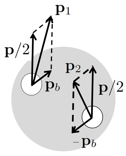
Figure 1: Quark positions and momenta inside a meson in its rest frame.

A simple choice of the meson wave function $\varphi_{\mathrm{M}}\left(\mathbf{k}\right)$ is the Gaussian distribution Greco et al. (2003); Fries et al. (2003)

$$\varphi_{\mathrm{M}}\left(\mathbf{k}\right)=\left(\frac{2\sqrt{\pi}}{a_{\mathrm{M}}}\right)^{3/2}\exp\left(-\frac{\mathbf{k}^{2}}{2a_{\mathrm{M}}^{2}}\right),$$ (14)

where $a_{\mathrm{M}}$ is the momentum width parameter of the meson. If we use the above Gaussian form of the wave function we can complete the integral over $\mathbf{q}_{b}$ in (13) to obtain the most simple form

$$\rho_{S_{z1},S_{z2}}^{\mathrm{M}}(\mathbf{x},\mathbf{p}) = \frac{1}{\pi^{3}}\int d^{3}\mathbf{x}_{b}d^{3}\mathbf{p}_{b}\exp\left(-\frac{\mathbf{p}_{b}^{2}}{a_{\mathrm{M}}^{2}}-a_{\mathrm{M}}^{2}\mathbf{x}_{b}^{2}\right)$$ (15)

$$\times\sum_{s_{1},s_{2}}w\left(\mathrm{q}_{1}\left|s_{1},\mathbf{x}_{1},\mathbf{p}_{1}\right.\right)w\left(\bar{\mathrm{q}}_{2}\left|s_{2},\mathbf{x}_{2},\mathbf{p}_{2}\right.\right)$$

$$\times\left\langle S,S_{z1}\mid s_{1},s_{2}\right\rangle\left\langle s_{1},s_{2}\mid S,S_{z2}\right\rangle.$$

We see that the Gaussian wave packet form appears in the integral which depends on the relative position and relative momentum between the quark and the antiquark.

Now we apply (15) to the vector meson $\phi$ with $S=1$ and $S_{z}=-1,0,1$. The diagonal elements of the spin density matrix for $\phi$ mesons are given in Eq. (57). With spin Wigner functions (11), the normalization condition (8) reads

$$\int d^{3}\mathbf{x}\int[d^{3}\mathbf{p}]f_{\mathrm{q}/\bar{\mathrm{q}}}(\mathbf{x},\mathbf{p})=1.$$ (16)

Since we are concerned mainly with polarization functions that are small $P_{\mathrm{q}/\bar{\mathrm{q}}}(\mathbf{x},\mathbf{p})\ll 1$, without loss of generality, we can assume $f_{\mathrm{q}}(\mathbf{x},\mathbf{p})=f_{\mathrm{q}}$ and $f_{\mathrm{\bar{q}}}(\mathbf{x},\mathbf{p})=f_{\mathrm{\bar{q}}}$ are constants. Under these assumptions, with (57) we obtain

$$\bar{\rho}_{00}^{\phi} = \frac{\rho_{00}^{\phi}(\mathbf{x},\mathbf{p})}{\rho_{00}^{\phi}(\mathbf{x},\mathbf{p})+\rho_{11}^{\phi}(\mathbf{x},\mathbf{p})+\rho_{-1,-1}^{\phi}(\mathbf{x},\mathbf{p})}$$ (17)

$$\approx \frac{1}{3}-\frac{4}{9}\left\langle P_{\mathrm{s}}\left(\mathbf{x}_{1},\mathbf{p}_{1}\right)P_{\bar{\mathrm{s}}}\left(\mathbf{x}_{2},\mathbf{p}_{2}\right)\right\rangle_{\phi},$$

where the average $\left\langle\cdots\right\rangle_{\mathrm{M}}$ is taken on the meson wave packet

$$\left\langle\cdots\right\rangle_{\mathrm{M}}\equiv\frac{1}{\pi^{3}}\int d^{3}\mathbf{x}_{b}d^{3}\mathbf{p}_{b}\exp\left(-\frac{\mathbf{p}_{b}^{2}}{a_{\mathrm{M}}^{2}}-a_{\mathrm{M}}^{2}\mathbf{x}_{b}^{2}\right)(\cdots).$$ (18)

If $P_{\mathrm{s}/\bar{\mathrm{s}}}$ are independent of positions, we can recover the result of Ref. Yang et al. (2018). In the remainder of this paper we will reuse $\rho_{00}^{\mathrm{M}}$ to denote the normalized $\bar{\rho}_{00}^{\mathrm{M}}$ for simplicity of notation.

In the same way, we can also obtain the normalized $\rho_{00}$ for the vector meson $K^{*0}$ with the flavor content $(\mathrm{d\bar{s}})$

$$\rho_{00}^{K^{*}} \approx \frac{1}{3}-\frac{4}{9}\left\langle P_{\mathrm{d}}\left(\mathbf{x}_{1},\mathbf{p}_{1}\right)P_{\bar{\mathrm{s}}}\left(\mathbf{x}_{2},\mathbf{p}_{2}\right)\right\rangle_{K^{*}}.$$ (19)

The result for $\overline{K}^{*0}$ with the flavor content $(\mathrm{s\bar{d}})$ can be obtained similarly.

II.2 Baryons

In this subsection we will derive the spin density matrix for baryons in phase space. The starting point is the spin density operator for three quarks. The spin, flavor and momentum part of the wave function for three quarks is the direct product of that for each single quark,

$$\left|\mathrm{q}_{1},\mathrm{q}_{2},\mathrm{q}_{3};s_{1},s_{2},s_{3};\mathbf{p}_{1},\mathbf{p}_{2},\mathbf{p}_{3}\right\rangle \equiv \left|\mathrm{q}_{1},s_{1},\mathbf{p}_{1}\right\rangle\left|\mathrm{q}_{2},s_{2},\mathbf{p}_{2}\right\rangle\left|\mathrm{q}_{3},s_{3},\mathbf{p}_{3}\right\rangle$$ (20)

$$= \left|\mathrm{q}_{1},\mathrm{q}_{2},\mathrm{q}_{3};s_{1},s_{2},s_{3}\right\rangle\left|\mathbf{p}_{1},\mathbf{p}_{2},\mathbf{p}_{3}\right\rangle,$$

where $s_{1,2,3}=\pm 1/2$ denote spins in the quantization direction and $\mathrm{q}_{1,2,3}=\mathrm{u},\mathrm{d},\mathrm{s}$ denote the spin states in the z-direction and quark flavors respectively. The second equality implies that the spin and flavor part of the wave function for three quarks is independent of the momentum part. The spin density operator for three quarks has the form

$$\rho_{\mathrm{qqq}} = \sum_{s_{1},s_{2},s_{3}}\sum_{\mathrm{q}_{1},\mathrm{q}_{2},\mathrm{q}_{3}}\int\prod_{i=1}^{3}d^{3}\mathbf{x}_{i}\prod_{i=1}^{3}[d^{3}\mathbf{p}_{i}]\prod_{i=1}^{3}[d^{3}\mathbf{q}_{i}]$$ (21)

$$\times\prod_{i=1}^{3}w(\mathrm{q}_{i}|s_{i},\mathbf{x}_{i},\mathbf{p}_{i})e^{-i\mathbf{q}_{i}\cdot\mathbf{x}_{i}}$$

$$\times\left|\mathrm{q}_{1},\mathrm{q}_{2},\mathrm{q}_{3};s_{1},s_{2},s_{3};\mathbf{p}_{1}+\frac{\mathbf{q}_{1}}{2},\mathbf{p}_{2}+\frac{\mathbf{q}_{2}}{2},\mathbf{p}_{3}+\frac{\mathbf{q}_{3}}{2}\right\rangle$$

$$\times\left\langle\mathrm{q}_{1},\mathrm{q}_{2},\mathrm{q}_{3};s_{1},s_{2},s_{3};\mathbf{p}_{1}-\frac{\mathbf{q}_{1}}{2},\mathbf{p}_{2}-\frac{\mathbf{q}_{2}}{2},\mathbf{p}_{3}-\frac{\mathbf{q}_{3}}{2}\right|.$$

The spin density matrix element for baryons with spin $S$ is given by putting $\rho_{\mathrm{qqq}}$ between two baryon states

$$\rho_{S_{z1},S_{z2}}^{\mathrm{B}}(\mathbf{x},\mathbf{p})=\int[d^{3}\mathbf{q}]e^{i\mathbf{q}\cdot\mathbf{x}}\left\langle\mathrm{B};S,S_{z1};\mathbf{p}+\frac{\mathbf{q}}{2}\right|\rho_{\mathrm{qqq}}\left|\mathrm{B};S,S_{z2};\mathbf{p}-\frac{\mathbf{q}}{2}\right\rangle.$$ (22)

For ground state (spin-1/2 octet and spin-3/2 decuplet) baryons, the spin-flavor part of the wave function is decoupled from the momentum or spatial part, but for excited states of baryons, they are generally entangled. In this paper we only consider ground state baryons so the momentum or spatial part of the baryon wave function is disentangled from the spin-flavor part. Using the Gaussian form of the baryon momentum wave function, we obtain

$$\rho_{S_{z1},S_{z2}}^{\mathrm{B}}(\mathbf{x},\mathbf{p}) = \frac{1}{\pi^{6}}\int d^{3}\mathbf{x}_{b}d^{3}\mathbf{x}_{c}d^{3}\mathbf{p}_{b}d^{3}\mathbf{p}_{c}$$ (23)

$$\times\exp\left(-\frac{\mathbf{p}_{b}^{2}}{a_{\mathrm{B}1}^{2}}-\frac{\mathbf{p}_{c}^{2}}{a_{\mathrm{B}2}^{2}}-a_{\mathrm{B}1}^{2}\mathbf{x}_{b}^{2}-a_{\mathrm{B}2}^{2}\mathbf{x}_{c}^{2}\right)$$

$$\times\sum_{s_{1},s_{2},s_{3}}\sum_{\mathrm{q}_{1},\mathrm{q}_{2},\mathrm{q}_{3}}$$

$$\times w\left(\mathrm{q}_{1}\left|s_{1},\mathbf{x}_{1},\mathbf{p}_{1}\right.\right)w\left(\mathrm{q}_{2}\left|s_{2},\mathbf{x}_{2},\mathbf{p}_{2}\right.\right)w\left(\mathrm{q}_{3}\left|s_{3},\mathbf{x}_{3},\mathbf{p}_{3}\right.\right)$$

$$\times\left\langle B;S,S_{z1}\right.\left|\mathrm{q}_{1},\mathrm{q}_{2},\mathrm{q}_{3};s_{1},s_{2},s_{3}\right\rangle$$

$$\times\left\langle\mathrm{q}_{1},\mathrm{q}_{2},\mathrm{q}_{3};s_{1},s_{2},s_{3}\right|\left.B;S,S_{z2}\right\rangle,$$

where $\mathbf{p}_{i}$ and $\mathbf{x}_{i}$ ($i=1,2,3$) are expressed in terms of Jacobi variables $\mathbf{p}_{j}$ and $\mathbf{x}_{j}$ ($j=a,b,c$) defined in Eq. (60) and (63) respectively and finally by setting $\mathbf{x}_{a}=\mathbf{x}$ and $\mathbf{p}_{a}=\mathbf{p}$, see Fig. 2 for illustration of positions of three quarks inside a baryon. The detailed derivation of (23) is given in Appendix C. We see that the wave packet form of the baryon emerges as a function of relative coordinates and relative momenta of three quarks.

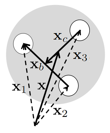
Figure 2: Positions of three quarks inside a baryon. The momenta conjugate to Jocobi cooridinates $\mathbf{x}_{a}=\mathbf{x}$, $\mathbf{x}_{b}$ and $\mathbf{x}_{c}$ are $\mathbf{p}_{a}$, $\mathbf{p}_{b}$ and $\mathbf{p}_{c}$ respectively, see Eq. (60) and (63).

As an example, we can apply (23) to the octet baryon $\Lambda$ with its SU(6) spin-flavor wave function. The spin-flavor wave function of $\Lambda$ tells that its spin in the quantization direction is carried by the s-quark while spins of u- and d-quark cancel. Similar to mesons, we also assume the polarization is small, $P_{\mathrm{q}/\bar{\mathrm{q}}}(\mathbf{x},\mathbf{p})\ll 1$ and $f_{\mathrm{q}}(\mathbf{x},\mathbf{p})=f_{\mathrm{q}}$ and $f_{\mathrm{\bar{q}}}(\mathbf{x},\mathbf{p})=f_{\mathrm{\bar{q}}}$ are constants. The result for the diagonal element of the spin density matrix $\rho_{++}^{\Lambda}\equiv\rho_{\frac{1}{2},\frac{1}{2}}^{\Lambda}$ is then

$$\rho_{++}^{\Lambda}(\mathbf{x},\mathbf{p}) = \frac{1}{24\pi^{6}}f_{\mathrm{u}}f_{\mathrm{d}}\int d^{3}\mathbf{x}_{b}d^{3}\mathbf{x}_{c}d^{3}\mathbf{p}_{b}d^{3}\mathbf{p}_{c}$$ (24)

$$\times\exp\left(-\frac{\mathbf{p}_{b}^{2}}{a_{\Lambda 1}^{2}}-\frac{\mathbf{p}_{c}^{2}}{a_{\Lambda 2}^{2}}-a_{\Lambda 1}^{2}\mathbf{x}_{b}^{2}-a_{\Lambda 2}^{2}\mathbf{x}_{c}^{2}\right)$$

$$\times\left\{w\left(\mathrm{s}\left|+,\mathbf{x}_{1},\mathbf{p}_{1}\right.\right)\left[2-P_{\mathrm{u}}(\mathbf{x}_{2},\mathbf{p}_{2})P_{\mathrm{d}}(\mathbf{x}_{3},\mathbf{p}_{3})-P_{\mathrm{u}}(\mathbf{x}_{3},\mathbf{p}_{3})P_{\mathrm{d}}(\mathbf{x}_{2},\mathbf{p}_{2})\right]\right.$$

$$+w\left(\mathrm{s}\left|+,\mathbf{x}_{2},\mathbf{p}_{2}\right.\right)\left[2-P_{\mathrm{u}}(\mathbf{x}_{3},\mathbf{p}_{3})P_{\mathrm{d}}(\mathbf{x}_{1},\mathbf{p}_{1})-P_{\mathrm{u}}(\mathbf{x}_{1},\mathbf{p}_{1})P_{\mathrm{d}}(\mathbf{x}_{3},\mathbf{p}_{3})\right]$$

$$+\left.w\left(\mathrm{s}\left|+,\mathbf{x}_{3},\mathbf{p}_{3}\right.\right)\left[2-P_{\mathrm{u}}(\mathbf{x}_{1},\mathbf{p}_{1})P_{\mathrm{d}}(\mathbf{x}_{2},\mathbf{p}_{2})-P_{\mathrm{u}}(\mathbf{x}_{2},\mathbf{p}_{2})P_{\mathrm{d}}(\mathbf{x}_{1},\mathbf{p}_{1})\right]\right\}.$$

Another diagonal element $\rho_{--}^{\Lambda}\equiv\rho_{-\frac{1}{2},-\frac{1}{2}}^{\Lambda}$ can be obtained from $\rho_{++}^{\Lambda}\equiv\rho_{\frac{1}{2},\frac{1}{2}}^{\Lambda}$ by flipping the s-quark’s spin, i.e. $w\left(\mathrm{s}\left|+,\mathbf{x}_{i},\mathbf{p}_{i}\right.\right)\rightarrow w\left(\mathrm{s}\left|-,\mathbf{x}_{i},\mathbf{p}_{i}\right.\right)$ with $i=1,2,3$. Finally we can read out the polarization of $\Lambda$ from spin density matrix elements

$$P_{\Lambda}(\mathbf{x},\mathbf{p}) = \frac{\rho_{++}^{\Lambda}(\mathbf{x},\mathbf{p})-\rho_{--}^{\Lambda}(\mathbf{x},\mathbf{p})}{\rho_{++}^{\Lambda}(\mathbf{x},\mathbf{p})+\rho_{--}^{\Lambda}(\mathbf{x},\mathbf{p})}$$ (25)

$$\approx \frac{1}{3}\left\langle P_{\mathrm{s}}(\mathbf{x}_{1},\mathbf{p}_{1})+P_{\mathrm{s}}(\mathbf{x}_{2},\mathbf{p}_{2})+P_{\mathrm{s}}(\mathbf{x}_{3},\mathbf{p}_{3})\right\rangle_{\Lambda},$$

where the average $\left\langle O(\mathbf{x}_{i},\mathbf{p}_{i})\right\rangle_{\mathrm{B}}$ with $i=1,2,3$ are taken on the wave packet function of baryons

$$\left\langle O(\mathbf{x}_{i},\mathbf{p}_{i})\right\rangle_{\mathrm{B}} \equiv \frac{1}{\pi^{6}}\int d^{3}\mathbf{x}_{b}d^{3}\mathbf{x}_{c}d^{3}\mathbf{p}_{b}d^{3}\mathbf{p}_{c}\>O(\mathbf{x}_{i},\mathbf{p}_{i})$$ (26)

$$\times\exp\left(-\frac{\mathbf{p}_{b}^{2}}{a_{\mathrm{B}1}^{2}}-\frac{\mathbf{p}_{c}^{2}}{a_{\mathrm{B}2}^{2}}-a_{\mathrm{B}1}^{2}\mathbf{x}_{b}^{2}-a_{\mathrm{B}2}^{2}\mathbf{x}_{c}^{2}\right).$$

Note that the integral in the average is normalized to 1, i.e. $\left\langle 1\right\rangle=1$.

III Spin polarization of quarks

In the last section we have constructed an improved quark coalescence model in phase space. The model is based on the spin density operator for quarks with spin dependent Wigner functions as weights, from which one can obtain spin density matrix elements in phase space for mesons and baryons. Once spin polarization functions for quarks in phase space (or equivalently spin Wigner functions) are known, one can calculate a vector meson’s spin alignment and a hyperon’s polarization.

There are different sources of spin polarization for massive fermions: vorticity fields, electromagnetic fields, and mean fields of vector mesons. The first two sources, vorticity and electromagnetic fields, have been extensively studied in quantum kinetic approach through Wigner functions Fang et al. (2016); Becattini et al. (2017); Weickgenannt et al. (2019); Gao and Liang (2019); Hattori et al. (2019); Wang et al. (2019); Liu et al. (2020). The polarization effect by vector meson fields was first proposed in Ref. Csernai et al. (2019) in the study of $\Lambda$ polarization. It was generalized to the spin alignment of vector mesons in Ref. Sheng et al. (2020). For each kind of field, one can distinguish the electric and magnetic part. It is believed that the contribution from electromagnetic fields is negligible Csernai et al. (2019); Sheng et al. (2020). Therefore in the remainder of this paper we consider vorticity and vector meson fields as main sources of spin polarization.

The spin polarization distribution in phase space for quarks (upper sign) and antiquarks (lower sign) is in the form Yang et al. (2018); Sheng et al. (2020)

$$P_{\pm}^{\mu}(x,p) = \frac{1}{2m}\left(\tilde{\omega}_{\mathrm{th}}^{\mu\nu}\pm\frac{g_{V}}{E_{p}T}\tilde{F}_{V}^{\mu\nu}\right)p_{\nu}\left[1-f_{FD}(E_{p}\mp\mu)\right],$$ (27)

where $p^{\mu}=(E_{p},\pm\mathbf{p})$ are on-shell momenta of quarks and antiquarks with $E_{p}=\sqrt{\mathbf{p}^{2}+m_{\mathrm{q}}^{2}}$, $\tilde{\omega}_{\mathrm{th}}^{\mu\nu}=\frac{1}{2}\epsilon^{\mu\nu\sigma\rho}\omega_{\sigma\rho}^{\mathrm{th}}$ is the dual of the thermal vorticity tensor defined by $\omega_{\sigma\rho}^{\mathrm{th}}=\frac{1}{2}[\partial_{\sigma}(\beta u_{\rho})-\partial_{\rho}(\beta u_{\sigma})]$ with $\beta\equiv 1/T$ being the temperature inverse (note that there is a sign difference in the definition of $\omega_{\sigma\rho}^{\mathrm{th}}$ from Ref. Becattini et al. (2013a)), $\tilde{F}_{V}^{\mu\nu}=\frac{1}{2}\epsilon^{\mu\nu\sigma\rho}F_{\sigma\rho}^{V}$ is the dual of the field strength tensor of vector mesons, and $f_{FD}$ is the Fermi-Dirac distribution. The electric and magnetic part of vector meson fields as three-vectors are defined as $\mathbf{E}_{V}^{i}=\mathbf{E}_{i}^{V}=F_{V}^{i0}$ and $\mathbf{B}_{V}^{i}=\mathbf{B}_{i}^{V}=-\frac{1}{2}\epsilon_{ijk}F_{V}^{jk}$ respectively with $i,j,k=x,y,z$. In a similar way, one can define the three-vector of thermal vorticity as $\boldsymbol{\omega}^{i}=\boldsymbol{\omega}_{i}=\tilde{\omega}_{\mathrm{th}}^{i0}$ which is the magnetic part of the thermal vorticity tensor, while the electric part of the thermal vorticity tensor is $\boldsymbol{\varepsilon}^{i}=\boldsymbol{\varepsilon}_{i}=\omega_{\mathrm{th}}^{i0}$. Written explicitly in three-vector forms, they are

$$\boldsymbol{\omega} = \frac{1}{2}\nabla\times(\beta\mathbf{u}),$$

$$\boldsymbol{\varepsilon} = -\frac{1}{2}[\partial_{t}(\beta\mathbf{u})+\nabla(\beta u^{0})].$$ (28)

We take $xz$ plane as the reaction plane with one nucleus moving along $+z$ direction at $x=-b/2$ while the other nucleus moving along $-z$ direction at $x=b/2$. The global OAM is along $+y$ direction. Therefore we assume that the spin quantization direction is $+y$, and that the Wigner functions in (11) are diagonalized in $+y$ direction. Then the polarization distribution for $\mathrm{q}$ and $\bar{\mathrm{q}}$ along $+y$ direction can be written as Sheng et al. (2020)

$$P_{\mathrm{q}/\bar{\mathrm{q}}}^{y}(\mathbf{x},\mathbf{p}) = \frac{1}{2}\boldsymbol{\omega}_{y}\pm\frac{1}{2m_{\mathrm{q}}}(\boldsymbol{\varepsilon}\times\mathbf{p})_{y}$$ (29)

$$\pm\frac{g_{V}}{2m_{\mathrm{q}}T}\mathbf{B}_{y}^{V}+\frac{g_{V}}{2m_{\mathrm{q}}E_{p}T}\left(\mathbf{E}_{V}\times\mathbf{p}\right)_{y},$$

where $g_{V}$ is the coupling constant of quarks and antiquarks to vector meson fields, and we have taken the Boltzmann limit $1-f_{FD}(E_{p}\mp\mu)\simeq 1$. The last term of Eq. (29) is the spin-orbit term for quarks and antiquarks involving the electric part of vector meson fields, the similar term is the key to the nuclear shell structure if applying to nucleons in meson fields Mayer (1949); Haxel et al. (1949). For $\mathrm{q}=\mathrm{s}$ and $\bar{\mathrm{q}}=\bar{\mathrm{s}}$, the vector meson field should be the $\phi$ field, i.e. $V=\phi$.

IV Global and local polarization of $\Lambda$

In this section we look at the polarization of $\Lambda$ (including $\bar{\Lambda}$ if not stated explicitly) in Eq. (25) with the polarization of s and $\bar{\mathrm{s}}$ given in Eq. (29). In this case the vector meson field is the $\phi$ field, i.e. $V=\phi$. By choosing $+y$ as the spin quantization direction, the spin polarization of $\Lambda$ and $\bar{\Lambda}$ in phase space is now

$$P_{\Lambda/\bar{\Lambda}}^{y}(\mathbf{x},\mathbf{p}) \approx \frac{1}{3}\left\langle P_{\mathrm{s}/\bar{\mathrm{s}}}^{y}(\mathbf{x}_{1},\mathbf{p}_{1})+P_{\mathrm{s}/\bar{\mathrm{s}}}^{y}(\mathbf{x}_{2},\mathbf{p}_{2})+P_{\mathrm{s}/\bar{\mathrm{s}}}^{y}(\mathbf{x}_{3},\mathbf{p}_{3})\right\rangle_{\Lambda/\bar{\Lambda}}$$ (30)

$$\approx \frac{1}{6}\left\langle\boldsymbol{\omega}_{y}(\mathbf{x}_{1})+\boldsymbol{\omega}_{y}(\mathbf{x}_{2})+\boldsymbol{\omega}_{y}(\mathbf{x}_{3})\right\rangle_{\Lambda/\bar{\Lambda}}$$

$$\pm\frac{1}{6m_{\mathrm{s}}}\hat{\mathbf{y}}\cdot\left\langle\boldsymbol{\varepsilon}(\mathbf{x}_{1})\times\mathbf{p}_{1}+\boldsymbol{\varepsilon}(\mathbf{x}_{2})\times\mathbf{p}_{2}+\boldsymbol{\varepsilon}(\mathbf{x}_{3})\times\mathbf{p}_{3}\right\rangle_{\Lambda/\bar{\Lambda}}$$

$$\pm\frac{g_{\phi}}{6m_{\mathrm{s}}T}\left\langle\mathbf{B}_{y}^{\phi}(\mathbf{x}_{1})+\mathbf{B}_{y}^{\phi}(\mathbf{x}_{2})+\mathbf{B}_{y}^{\phi}(\mathbf{x}_{3})\right\rangle_{\Lambda/\bar{\Lambda}}$$

$$+\frac{g_{\phi}}{6m_{\mathrm{s}}^{2}T}\hat{\mathbf{y}}\cdot\left\langle\mathbf{E}_{\phi}(\mathbf{x}_{1})\times\mathbf{p}_{1}+\mathbf{E}_{\phi}(\mathbf{x}_{2})\times\mathbf{p}_{2}+\mathbf{E}_{\phi}(\mathbf{x}_{3})\times\mathbf{p}_{3}\right\rangle_{\Lambda/\bar{\Lambda}}.$$

where we have taken non-relativistic limit $E_{p}\approx m_{\mathrm{s}}$. We can take an average over a space volume at the formation time of $\Lambda$. If all fields change slowly inside $\Lambda$, we can approximate $O(\mathbf{x}_{i})\approx O(\mathbf{x})$ for $i=1,2,3$. Then we obtain

$$\left\langle P_{\Lambda/\bar{\Lambda}}^{y}(\mathbf{x},\mathbf{p})\right\rangle \approx \frac{1}{2}\left\langle\boldsymbol{\omega}_{y}(\mathbf{x})\right\rangle\pm\frac{1}{6m_{\mathrm{s}}}\left[\left\langle\boldsymbol{\varepsilon}(\mathbf{x})\right\rangle\times\mathbf{p}\right]_{y}$$ (31)

$$\pm\frac{g_{\phi}}{2m_{\mathrm{s}}}\left\langle\beta\mathbf{B}_{y}^{\phi}(\mathbf{x})\right\rangle+\frac{g_{\phi}}{6m_{\mathrm{s}}^{2}}\left[\left\langle\beta\mathbf{E}_{\phi}(\mathbf{x})\right\rangle\times\mathbf{p}\right]_{y},$$

where $\left\langle\cdot\right\rangle$ represents the volume average at the formation time of $\Lambda$. Note that the spin-orbit term $\mathbf{E}_{\phi}\times\mathbf{p}$ has the same sign for $\Lambda$ and $\bar{\Lambda}$.

For static $\Lambda$ with $\mathbf{p}=0$, the terms involving $\boldsymbol{\varepsilon}$ and $\mathbf{E}_{\phi}$ are vanishing Sheng et al. (2020), but for non-static $\Lambda$ with non-vanishing momenta, they are generally present. However, for the global spin polarization in the direction of $+y$ (direction of the global OAM) with all $\Lambda$ and $\bar{\Lambda}$ in momentum spectra being included, these terms of $\boldsymbol{\varepsilon}$ and $\mathbf{E}_{\phi}$ are vanishing. So the global polarization for $\Lambda$ and $\bar{\Lambda}$ measured in STAR experiments Adamczyk et al. (2017); Adam et al. (2018) comes mainly from $\boldsymbol{\omega}_{y}$ and $\mathbf{B}_{y}^{\phi}$. Note that the $\mathbf{B}_{y}^{\phi}$ term for $\bar{\Lambda}$ has an opposite sign to $\Lambda$. This provides a possible explanation of the difference between magnitudes of $P_{\Lambda}^{y}$ and $P_{\bar{\Lambda}}^{y}$, similar to the scenario of Ref. Csernai et al. (2019). The fact $P_{\bar{\Lambda}}^{y}>P_{\Lambda}^{y}$ shown in experimental data indicates $g_{\phi}\left\langle\beta\mathbf{B}_{y}^{\phi}(\mathbf{x})\right\rangle<0$.

Recent STAR measurements Adam et al. (2019) of the longitudinal spin polarization of $\Lambda$ as functions show a positive $\sin\left(2\phi-2\Psi_{2}\right)$ behavior with $\phi$ and $\Psi_{2}$ being the azimuthal angle of $\Lambda$ and the second-order event plane respectively, while theoretical results of relativistic hydrodynamics model Becattini and Karpenko (2018) and transport models Xie et al. (2017); Xia et al. (2018); Wei et al. (2019) show an opposite sign. The simulation from chiral kinetic theory in Ref. Liu et al. (2019) and results from a simple phenomenological model in Ref. Voloshin (2018) gives the correct sign as the data. The sign problem in local polarization may indicate the assumption of global equilibrium of spin may not be justified, so the thermal vorticity may not be the right quantity for the spin chemical potential Wu et al. (2019). The azimuthal angle dependence of $P_{\Lambda/\bar{\Lambda}}^{y}$ has been measured by the STAR collaboration with the trend that $P_{\Lambda/\bar{\Lambda}}^{y}$ in the reaction plane is larger than that out of the reaction plane. This phenomenon has not been well understood Wu et al. (2019).

The spin-orbit term may provide an additional contribution to the polarization along the beam direction $P_{\Lambda/\bar{\Lambda}}^{z}$ in heavy ion collisions Adam et al. (2019). To this end, we split the whole space into four parts corresponding to four quadrants of the transverse plane which we denote as $++$, $-+$, $--$ and $+-$ respectively. Let us look at $\left\langle P_{\Lambda/\bar{\Lambda}}^{z}\right\rangle$ in the first and second quadrant

$$\left\langle P_{\Lambda/\bar{\Lambda}}^{z}(\mathbf{x},\mathbf{p})\right\rangle_{++} \sim \frac{g_{\phi}}{2m_{\mathrm{s}}^{2}}\left[\left\langle\beta\mathbf{E}_{\phi}^{x}\right\rangle_{++}p_{T}\sin(\phi_{p})-\left\langle\beta\mathbf{E}_{\phi}^{y}\right\rangle_{++}p_{T}\cos(\phi_{p})\right],$$

$$\left\langle P_{\Lambda/\bar{\Lambda}}^{z}(\mathbf{x},\mathbf{p})\right\rangle_{-+} \sim \frac{g_{\phi}}{2m_{\mathrm{s}}^{2}}\left[\left\langle\beta\mathbf{E}_{\phi}^{x}\right\rangle_{-+}p_{T}\sin(\phi_{p})-\left\langle\beta\mathbf{E}_{\phi}^{y}\right\rangle_{-+}p_{T}\cos(\phi_{p})\right].$$ (32)

If $\left\langle\beta\mathbf{E}_{\phi}\right\rangle$ is dominated by the $x$ component in the first and second quadrant and if $g_{\phi}\left\langle\beta\mathbf{E}_{\phi}^{x}\right\rangle_{++}=-g_{\phi}\left\langle\beta\mathbf{E}_{\phi}^{x}\right\rangle_{-+}>0$, then we can obtain the patterns observed in experiments Adam et al. (2019): $\left\langle P_{\Lambda/\bar{\Lambda}}^{y}(\mathbf{x},\mathbf{p})\right\rangle_{++}>0$ and $\left\langle P_{\Lambda/\bar{\Lambda}}^{y}(\mathbf{x},\mathbf{p})\right\rangle_{-+}<0$.

Furthermore the spin-orbit term $\mathbf{E}_{\phi}\times\mathbf{p}$ in $P_{\Lambda/\bar{\Lambda}}^{y}$ may also provide a possible additional contribution to the azimuthal angle dependence of the polarization along $+y$ in heavy ion collisions Niida (2019), if there is a correlation between $\mathbf{E}_{\phi}$ and $\mathbf{p}$ in a certain region. In order to look at the relevant observable, we choose the region for taking average to be $x>0,y>0$ corresponding to the first quadrant of the transverse plane in collisions, the average quantity is denoted as $\left\langle\beta\mathbf{E}_{\phi}\right\rangle_{++}$ which may not be vanishing (the average of $\beta\mathbf{E}_{\phi}$ over the full space should be vanishing). Then the azimuthal angle part of $P_{\Lambda/\bar{\Lambda}}^{y}$ in the first quadrant of the transverse plane is

$$\left\langle P_{\Lambda/\bar{\Lambda}}^{y}(\mathbf{x},\mathbf{p})\right\rangle_{++}\sim\frac{g_{\phi}}{2m_{\mathrm{s}}^{2}}\left\langle\beta\mathbf{E}_{\phi}^{z}\right\rangle_{++}p_{T}\cos(\phi_{p}),$$ (33)

where $\phi_{p}$ is the azimuthal angle relative to that of the reaction plane, and $p_{T}\equiv|\mathbf{p}_{T}|$ is the scalar transverse momentum. We see that the spin-orbit term may provide an additional contribution to the the azimuthal angle dependence of $P_{\Lambda/\bar{\Lambda}}^{y}$.

V Spin alignments of $\phi$ and $K^{*0}$

We now investigate spin alignments of vector mesons $\phi$ and $K^{*0}$. In the remainder of this paper, when we say $K^{*0}$ we imply to include $\overline{K}^{*0}$ if there is no ambiguity.

Let us first look at the spin alignment of $\phi$. Substituting Eq. (29) for $\mathrm{q}=\mathrm{s}$ and $\bar{\mathrm{q}}=\bar{\mathrm{s}}$ into Eq. (17) and taking an average on a space volume, we obtain the spin density matrix element for $\phi$ mesons

$$\left\langle\rho_{00}^{\phi}(\mathbf{x},\mathbf{p})\right\rangle \approx \frac{1}{3}-\frac{4}{9}\left\langle P_{\mathrm{s}}^{y}\left(\mathbf{x}_{1},\mathbf{p}_{1}\right)P_{\bar{\mathrm{s}}}^{y}\left(\mathbf{x}_{2},\mathbf{p}_{2}\right)\right\rangle_{\phi,\mathrm{Vol}}$$ (34)

$$\approx \frac{1}{3}-\frac{1}{9}\left\langle\boldsymbol{\omega}_{y}^{2}\right\rangle+\frac{1}{9m_{s}^{2}}\left\langle\left(\boldsymbol{\varepsilon}\times\mathbf{p}_{1}\right)_{y}\left(\boldsymbol{\varepsilon}\times\mathbf{p}_{2}\right)_{y}\right\rangle_{\phi,\mathrm{Vol}}$$

$$+\frac{g_{\phi}^{2}}{9m_{\mathrm{s}}^{2}}\left\langle\left(\beta\mathbf{B}_{y}^{\phi}\right)^{2}\right\rangle-\frac{g_{\phi}^{2}}{9m_{\mathrm{s}}^{2}}\left\langle\frac{\beta^{2}}{E_{p1}E_{p2}}\left(\mathbf{E}_{\phi}\times\mathbf{p}_{1}\right)_{y}\left(\mathbf{E}_{\phi}\times\mathbf{p}_{2}\right)_{y}\right\rangle_{\phi,\mathrm{Vol}},$$

where the spin quantization direction is chosen as $+y$, $\left\langle\cdot\right\rangle$ denotes the volume average at the formation time of $\phi$ mesons, and we have put index ’Vol’ to distinguish the volume average from the average on the $\phi$ meson wave function if both averages are taken. In deriving Eq. (34) we have made approximations: (a) The size of the vector meson is much smaller than the hydrodynamic scale, so we put $\mathbf{x}_{1}\approx\mathbf{x}_{2}\approx\mathbf{x}$ for vorticity fields and the $\phi$ fields; (b) We neglect correlation in the volume between different fields except between themselves Sheng et al. (2020), for example, no correlation between $\mathbf{E}_{\phi}$ and $\mathbf{B}_{\phi}$, between $\boldsymbol{\varepsilon}$ and $\mathbf{E}_{\phi}$, or between $\boldsymbol{\omega}$ and $\mathbf{B}_{\phi}$, etc.. We also neglect correlation in the volume between different components of the same field, for example, between $\mathbf{E}_{\phi}^{x}$ and $\mathbf{E}_{\phi}^{z}$ or between $\boldsymbol{\varepsilon}_{z}$ and $\boldsymbol{\varepsilon}_{x}$, etc..

We now simplify terms involving $\boldsymbol{\varepsilon}$ and $\mathbf{E}_{\phi}$ in (34). The $\boldsymbol{\varepsilon}$ term is evaluated as

$$\left\langle\left(\boldsymbol{\varepsilon}\times\mathbf{p}_{1}\right)_{y}\left(\boldsymbol{\varepsilon}\times\mathbf{p}_{2}\right)_{y}\right\rangle_{\phi,\mathrm{Vol}}$$ (35)

$$\approx \frac{1}{4}\left\langle\boldsymbol{\varepsilon}_{z}^{2}\right\rangle\mathbf{p}_{x}^{2}+\frac{1}{4}\left\langle\boldsymbol{\varepsilon}_{x}^{2}\right\rangle\mathbf{p}_{z}^{2}-\left\langle\boldsymbol{\varepsilon}_{z}^{2}\right\rangle\left\langle\mathbf{p}_{b,x}^{2}\right\rangle_{\phi}-\left\langle\boldsymbol{\varepsilon}_{x}^{2}\right\rangle\left\langle\mathbf{p}_{b,z}^{2}\right\rangle_{\phi}$$

$$= \frac{1}{4}\left\langle\boldsymbol{\varepsilon}_{z}^{2}\right\rangle\mathbf{p}_{x}^{2}+\frac{1}{4}\left\langle\boldsymbol{\varepsilon}_{x}^{2}\right\rangle\mathbf{p}_{z}^{2}-\frac{1}{3}\left(\left\langle\boldsymbol{\varepsilon}_{z}^{2}\right\rangle+\left\langle\boldsymbol{\varepsilon}_{x}^{2}\right\rangle\right)\left\langle\mathbf{p}_{b}^{2}\right\rangle_{\phi},$$

and the $\mathbf{E}_{\phi}$ term is evaluated as

$$\left\langle\frac{\beta^{2}}{E_{p1}E_{p2}}\left(\mathbf{E}_{\phi}\times\mathbf{p}_{1}\right)_{y}\left(\mathbf{E}_{\phi}\times\mathbf{p}_{2}\right)_{y}\right\rangle_{\phi,\mathrm{Vol}}$$ (36)

$$\approx \frac{1}{4}\left\langle\beta^{2}\mathbf{E}_{\phi,z}^{2}\right\rangle\left\langle\frac{1}{E_{p1}E_{p2}}\right\rangle_{\phi}\mathbf{p}_{x}^{2}+\frac{1}{4}\left\langle\beta^{2}\mathbf{E}_{\phi,x}^{2}\right\rangle\left\langle\frac{1}{E_{p1}E_{p2}}\right\rangle_{\phi}\mathbf{p}_{z}^{2}$$

$$-\left\langle\beta^{2}\mathbf{E}_{\phi,z}^{2}\right\rangle\left\langle\frac{\mathbf{p}_{b,x}^{2}}{E_{p1}E_{p2}}\right\rangle_{\phi}-\left\langle\beta^{2}\mathbf{E}_{\phi,x}^{2}\right\rangle\left\langle\frac{\mathbf{p}_{b,z}^{2}}{E_{p1}E_{p2}}\right\rangle_{\phi},$$

where we have used $\mathbf{p}_{1,2}=\mathbf{p}/2\pm\mathbf{p}_{b}$ and dropped terms with mixture of different fields or different components of the same field. Inserting (35) and (36) into (34) we obtain

$$\left\langle\rho_{00}^{\phi}(\mathbf{x},\mathbf{p})\right\rangle \approx \frac{1}{3}-\frac{1}{9}\left\langle\boldsymbol{\omega}_{y}^{2}\right\rangle-\frac{1}{27m_{s}^{2}}\left(\left\langle\boldsymbol{\varepsilon}_{z}^{2}\right\rangle+\left\langle\boldsymbol{\varepsilon}_{x}^{2}\right\rangle\right)\left\langle\mathbf{p}_{b}^{2}\right\rangle_{\phi}$$ (37)

$$+\frac{g_{\phi}^{2}}{9m_{\mathrm{s}}^{2}}\left\langle\left(\beta\mathbf{B}_{y}^{\phi}\right)^{2}\right\rangle+\frac{g_{\phi}^{2}}{9m_{\mathrm{s}}^{2}}\left[\left\langle\beta^{2}\mathbf{E}_{\phi,z}^{2}\right\rangle\left\langle\frac{\mathbf{p}_{b,x}^{2}}{E_{p1}E_{p2}}\right\rangle_{\phi}+\left\langle\beta^{2}\mathbf{E}_{\phi,x}^{2}\right\rangle\left\langle\frac{\mathbf{p}_{b,z}^{2}}{E_{p1}E_{p2}}\right\rangle_{\phi}\right]$$

$$+\rho_{p}(\boldsymbol{\varepsilon}_{z}^{2})\mathbf{p}_{x}^{2}+\rho_{p}(\boldsymbol{\varepsilon}_{x}^{2})\mathbf{p}_{z}^{2}-\rho_{p}(\phi,\mathbf{E}_{\phi,z}^{2})\mathbf{p}_{x}^{2}-\rho_{p}(\phi,\mathbf{E}_{\phi,x}^{2})\mathbf{p}_{z}^{2},$$

where we have used following positive coefficients

$$\rho_{p}(\boldsymbol{\varepsilon}_{i}^{2}) = \frac{1}{36m_{s}^{2}}\left\langle\boldsymbol{\varepsilon}_{i}^{2}\right\rangle,$$

$$\rho_{p}(\phi,\mathbf{E}_{\phi,i}^{2}) = \frac{g_{\phi}^{2}}{36m_{\mathrm{s}}^{2}}\left\langle\beta^{2}\mathbf{E}_{\phi,i}^{2}\right\rangle\left\langle\frac{1}{E_{p1}E_{p2}}\right\rangle_{\phi},$$ (38)

with $i=x,y,z$. For nearly static $\phi$ mesons with $|\mathbf{p}|\ll|\mathbf{p}_{b}|$ the terms proportional to $\mathbf{p}_{x}^{2}$ and $\mathbf{p}_{z}^{2}$ in (37) are very small and can be neglected compared with the $\left\langle\mathbf{p}_{b}^{2}\right\rangle_{\phi}$ term, in this case we recover the result of Ref. Sheng et al. (2020) in nonrelativistic limit with $E_{p1}\approx E_{p2}\approx m_{\mathrm{s}}$

$$\left\langle\rho_{00}^{\phi}(\mathbf{x},\mathbf{p}\approx 0)\right\rangle \approx \frac{1}{3}-\frac{1}{9}\left\langle\boldsymbol{\omega}_{y}^{2}\right\rangle-\frac{1}{27m_{s}^{2}}\left(\left\langle\boldsymbol{\varepsilon}_{z}^{2}\right\rangle+\left\langle\boldsymbol{\varepsilon}_{x}^{2}\right\rangle\right)\left\langle\mathbf{p}_{b}^{2}\right\rangle_{\phi}$$ (39)

$$+\frac{g_{\phi}^{2}}{9m_{\mathrm{s}}^{2}}\left\langle\left(\beta\mathbf{B}_{y}^{\phi}\right)^{2}\right\rangle+\frac{g_{\phi}^{2}}{9m_{\mathrm{s}}^{4}}\left[\left\langle\beta^{2}\mathbf{E}_{\phi,z}^{2}\right\rangle\left\langle\mathbf{p}_{b,x}^{2}\right\rangle_{\phi}+\left\langle\beta^{2}\mathbf{E}_{\phi,x}^{2}\right\rangle\left\langle\mathbf{p}_{b,z}^{2}\right\rangle_{\phi}\right].$$

In Eq. (37) and (39) there are averages of squares of relative momenta of two quarks on the wave function of $\phi$ mesons and there are also space volume averages of field squares.

Equation (37) with (39) as its static limit is part of our main results in the paper. A few remarks are in order about Eq. (37): (a) All contributions appear independently as positive or negative quantities. This is the main feature of $\rho_{00}$ for $\phi$ mesons. (b) The second term is from the vorticity vector (magnetic part of the vorticity tensor), while the third term is from the electric part of the vorticity tensor. Both terms are negative definite. (c) The fourth term is from the magnetic part of the $\phi$ field, while the fifth term is from the electric part of the $\phi$ field. Both terms are positive definite. (d) The last line collects contributions proportional to momentum squares of the $\phi$ meson, where the contribution from the electric part of the vorticity tensor is always positive while that from the electric part of the $\phi$ field is always negative. (e) We have argued in Ref. Sheng et al. (2020) that the dominant contribution to $\rho_{00}^{\phi}$ may possibly be from the electric part of the $\phi$ field which is positive definite.

Let us turn to the spin alignment of another vector meson $K^{*0}$. Different from the $\phi$ meson with flavor content $(\mathrm{s}\bar{\mathrm{s}})$, $K^{*0}$ has flavor $(\mathrm{d\bar{s}})$. Vector meson ($\rho$ or $\omega$) fields that can polarize light quarks are different from the $\phi$ field which mainly polarize $\mathrm{s}$ and $\bar{\mathrm{s}}$. We will see that such a difference has significant consequences on $\rho_{00}^{K^{*}}$. Following the same procedure and taking the same approximations as in deriving (34), we obtain the spin density matrix element for $K^{*0}$, a counterpart of Eq. (37),

$$\left\langle\rho_{00}^{K^{*}}(\mathbf{x},\mathbf{p})\right\rangle \approx \frac{1}{3}-\frac{1}{9}\left\langle\boldsymbol{\omega}_{y}^{2}\right\rangle-\frac{1}{27m_{\mathrm{s}}m_{\mathrm{d}}}\left(\left\langle\boldsymbol{\varepsilon}_{z}^{2}\right\rangle+\left\langle\boldsymbol{\varepsilon}_{x}^{2}\right\rangle\right)\left\langle\mathbf{p}_{b}^{2}\right\rangle_{K^{*}}$$ (40)

$$+\frac{g_{\phi}g_{V}}{9m_{\mathrm{s}}m_{\mathrm{d}}}\left\langle\beta^{2}\mathbf{B}_{y}^{\phi}\mathbf{B}_{y}^{V}\right\rangle$$

$$+\frac{g_{\phi}g_{V}}{9m_{\mathrm{s}}m_{\mathrm{d}}}\left[\left\langle\beta^{2}\mathbf{E}_{z}^{\phi}\mathbf{E}_{z}^{V}\right\rangle\left\langle\frac{\mathbf{p}_{b,x}^{2}}{E_{p1}^{\mathrm{d}}E_{p2}^{\bar{\mathrm{s}}}}\right\rangle_{K^{*}}+\left\langle\beta^{2}\mathbf{E}_{x}^{\phi}\mathbf{E}_{x}^{V}\right\rangle\left\langle\frac{\mathbf{p}_{b,z}^{2}}{E_{p1}^{\mathrm{d}}E_{p2}^{\bar{\mathrm{s}}}}\right\rangle_{K^{*}}\right]$$

$$+\frac{m_{\mathrm{s}}}{m_{\mathrm{d}}}\rho_{p}(\boldsymbol{\varepsilon}_{z}^{2})\mathbf{p}_{x}^{2}+\frac{m_{\mathrm{s}}}{m_{\mathrm{d}}}\rho_{p}(\boldsymbol{\varepsilon}_{x}^{2})\mathbf{p}_{z}^{2}$$

$$-\rho_{p}(K^{*},\mathbf{E}_{z}^{\phi}\mathbf{E}_{z}^{V})\mathbf{p}_{x}^{2}-\rho_{p}(K^{*},\mathbf{E}_{x}^{\phi}\mathbf{E}_{x}^{V})\mathbf{p}_{z}^{2},$$

where $\mathbf{B}_{i}^{\phi}$ and $\mathbf{E}_{i}^{\phi}$ with $i=x,y,z$ are from the polarization of $\bar{\mathrm{s}}$, while $\mathbf{B}_{i}^{V}$ and $\mathbf{E}_{i}^{V}$ are vector meson fields ($\rho$ or $\omega$ mesons) that polarize the d-quark, and $\rho_{p}(K^{*},\mathbf{E}_{i}^{\phi}\mathbf{E}_{i}^{V})$ are defined as

$$\rho_{p}(K^{*},\mathbf{E}_{i}^{\phi}\mathbf{E}_{i}^{V})=\frac{g_{\phi}g_{V}}{36m_{\mathrm{s}}m_{\mathrm{d}}}\left\langle\beta^{2}\mathbf{E}_{i}^{\phi}\mathbf{E}_{i}^{V}\right\rangle\left\langle\frac{1}{E_{p1}^{\mathrm{d}}E_{p2}^{\bar{\mathrm{s}}}}\right\rangle_{K^{*}}.$$ (41)

In (40) we have shown terms of volume averages of different fields, $\left\langle\beta^{2}\mathbf{B}_{y}^{\phi}\mathbf{B}_{y}^{V}\right\rangle$ and $\left\langle\beta^{2}\mathbf{E}_{i}^{\phi}\mathbf{E}_{i}^{V}\right\rangle$, for the purpose of illustration and comparison, since they should have been neglected in accordance with the approximation that different fields do not have large correlation in space as compared with the correlation between the same fields. After implementing this approximation, we obtain

$$\left\langle\rho_{00}^{K^{*}}(\mathbf{x},\mathbf{p})\right\rangle \approx \frac{1}{3}-\frac{1}{9}\left\langle\boldsymbol{\omega}_{y}^{2}\right\rangle-\frac{1}{27m_{\mathrm{s}}m_{\mathrm{d}}}\left(\left\langle\boldsymbol{\varepsilon}_{z}^{2}\right\rangle+\left\langle\boldsymbol{\varepsilon}_{x}^{2}\right\rangle\right)\left\langle\mathbf{p}_{b}^{2}\right\rangle_{K^{*}}$$ (42)

$$+\frac{m_{\mathrm{s}}}{m_{\mathrm{d}}}\left[\rho_{p}(\boldsymbol{\varepsilon}_{z}^{2})\mathbf{p}_{x}^{2}+\rho_{p}(\boldsymbol{\varepsilon}_{x}^{2})\mathbf{p}_{z}^{2}\right].$$

We can see that the slope of $\rho_{00}^{K^{*}}$ with respect to $p_{T}^{2}$ is positive. For nearly static $K^{*0}$ mesons with $|\mathbf{p}|\ll|\mathbf{p}_{b}|$, the terms proportional to $\mathbf{p}_{x}^{2}$ and $\mathbf{p}_{z}^{2}$ in (37) are very small and can be neglected, then we have

$$\left\langle\rho_{00}^{K^{*}}(\mathbf{x},\mathbf{p}\approx 0)\right\rangle\approx\frac{1}{3}-\frac{1}{9}\left\langle\boldsymbol{\omega}_{y}^{2}\right\rangle-\frac{1}{27m_{\mathrm{s}}m_{\mathrm{d}}}\left(\left\langle\boldsymbol{\varepsilon}_{z}^{2}\right\rangle+\left\langle\boldsymbol{\varepsilon}_{x}^{2}\right\rangle\right)\left\langle\mathbf{p}_{b}^{2}\right\rangle_{K^{*}}.$$ (43)

We see in (42) and (43) the absence of the contribution from vector meson fields. Therefore the spin alignment of $K^{*0}$ is dominated by the vorticity contribution which must be negative for nearly static $K^{*0}$. This is the significant difference from the spin alignment of $\phi$ mesons which may possibly be dominated by $\phi$ fields whose contribution is positive definite for nearly static $\phi$ mesons. Another feature of $\rho_{00}^{K^{*}}$ in (42) and (43) is that the contribution from the electric part of the vorticity tensor is amplified by a factor $(m_{\mathrm{s}}/m_{\mathrm{d}})\left(\left\langle\mathbf{p}_{b}^{2}\right\rangle_{K^{*}}/\left\langle\mathbf{p}_{b}^{2}\right\rangle_{\phi}\right)$ compared with $\rho_{00}^{\phi}$. Note that the ratio $\left\langle\mathbf{p}_{b}^{2}\right\rangle_{K^{*}}/\left\langle\mathbf{p}_{b}^{2}\right\rangle_{\phi}$ is about $1.4\sim 1.5$ in the quark model. This may provide a sizable magnitude of the negative contribution to $\rho_{00}^{K^{*}}$ as shown in ALICE experiments Acharya et al. (2020).

We note that the above arguments are only valid for primary $K^{*0}$. The life time of $K^{*0}$ is much shorter and the interaction of $K^{*0}$ with the surrounding matter is much stronger than the $\phi$ meson. This may bring other contributions to $\rho_{00}^{K^{*}}$ from the interaction of $K^{*0}$ with medium. A caveat is that the above arguments are based on the approximation that different fields do not have large correlation in space as compared with the correlation between the same fields. This seems to work for $\rho_{00}^{\phi}$ since there are squares of the same vector meson field. However it is not the case for $\rho_{00}^{K^{*}}$ that all terms of vector meson fields are mixture of differenct fields which are thought to be equally small. In this case, in order to justify the approximation, we may need to evaluate these terms and compare their magnitudes with the negative comtribution from vorticity tensor fields. This is beyond the scope of this paper and will be studied in the future.

Figure 3: An example for the effects of vector meson fields on the spin density matrices of $\phi$ and $K^{*0}$ mesons in their rest frame. There is large correlation between vector meson fields acting on s and $\bar{\mathrm{s}}$ in the $\phi$ meson but almost no correlation between vector meson fields acting on d and $\bar{\mathrm{s}}$ in $K^{*0}$. Due to the short distance nature of vector meson fields, the dominant contribution to the fields at the position of a constituent quark of $\phi$ or $K^{*0}$ is from the quark of its nearest neighbor. The relative momentum of the quark and antiquark inside the meson is shown as $2\mathbf{p}$ (intead of $2\mathbf{p}_{b}$ in the text).

To summarize, in the picture of the coalescence model, we propose that a large positive contribution to the spin matrix element $\rho_{00}^{\phi}$ should be from the $\phi$ field Sheng et al. (2020). This is due to the correlation between the $\phi$ field that polarizes the s-quark and that polarizes $\bar{\mathrm{s}}$, see Fig. 3 for illustration. However this is not the case for $\rho_{00}^{K^{*}}$: the $\phi$ field that polarizes $\bar{\mathrm{s}}$ does not correlate much with vector meson fields ($\rho$ or $\omega$ mesons) that polarize the d-quark, the former is from other strange quarks not belonging to $K^{*0}$, while the latter come from other light quarks surrounding d, see Fig. 3. Therefore $\rho_{00}^{K^{*}}$ is dominated by the contribution from vorticity fields which is negative definite for static $K^{*0}$. Such a negative contribution from vorticity fields in $\rho_{00}^{K^{*}}$ is amplified relative to $\rho_{00}^{\phi}$ by the mass ratio of strange to light quark and by the ratio of $\left\langle\mathbf{p}_{b}^{2}\right\rangle$ on $K^{*0}$’s to $\phi$’s wave function.

VI Solving vector meson fields generated by sources

In this section we solve the mean vector field which satisfies the Klein-Gordon equation Csernai et al. (2019)

$$\partial_{\mu}F_{V}^{\mu\nu}+m_{V}^{2}V^{\nu}=g_{V}J^{\nu},$$ (44)

where $F_{V}^{\mu\nu}\equiv\partial^{\mu}V^{\nu}-\partial^{\nu}V^{\mu}$ is the field strength tensor, the source of the field $J^{\mu}$ is the current density associated with a conserved quantum number, $m_{V}$ is the vector meson mass, and $g_{V}$ is the coupling constant. We can write $V^{\mu}$ and $J^{\mu}$ explicitly as $V^{\mu}=(\phi,\mathbf{A})$ and $J^{\mu}=(\rho,\mathbf{j})$. We can also define the electric and magnetic part of $F_{V}^{\mu\nu}$ as three-vectors as in Sect. III. If $m_{V}$ is very large compared with the derivative term, we can just neglect latter in Eq. (44). In this case $V^{\mu}$ can be approximately proportional to the current density Csernai et al. (2019), $V^{\mu}\approx(g_{V}/m_{V}^{2})J^{\mu}$, known as the current-field identity Gell-Mann and Zachariasen (1961); Kroll et al. (1967) in the vector dominance model Sakurai (1960); Bauer et al. (1978).

We can use the Green’s function method to solve the Klein-Gordon equation (44) as to solve Maxwell’s equations in Ref. Li et al. (2016). The only difference is the presence of the vector meson mass which brings a little more complexity. We consider a point charge $Q$ located at the original point at $t=0$ moves with velocity $v$ in $+z$ direction. The charge $Q$ corresponds to a quantum number such as the baryon number for quarks or the strangeness number for $\mathrm{s}$ and $\bar{\mathrm{s}}$. Finally we obtain the electric and magnetic parts of vector meson fields as

$$\mathbf{E}_{V}^{x}(t,\mathbf{x}) = g_{V}Q\frac{\gamma v(1+m_{V}\Delta)}{4\pi\Delta^{3}}x\,e^{-m_{V}\Delta},$$

$$\mathbf{E}_{V}^{y}(t,\mathbf{x}) = g_{V}Q\frac{\gamma v(1+m_{V}\Delta)}{4\pi\Delta^{3}}y\,e^{-m_{V}\Delta},$$

$$\mathbf{E}_{V}^{z}(t,\mathbf{x}) = g_{V}Q\frac{\gamma v(1+m_{V}\Delta)}{4\pi\Delta^{3}}(z-vt)\,e^{-m_{V}\Delta},$$

$$\mathbf{B}_{V}^{x}(t,\mathbf{x}) = -g_{V}Q\frac{\gamma v(1+m_{V}\Delta)}{4\pi\Delta^{3}}y\,e^{-m_{V}\Delta},$$

$$\mathbf{B}_{V}^{y}(t,\mathbf{x}) = g_{V}Q\frac{\gamma v(1+m_{V}\Delta)}{4\pi\Delta^{3}}x\,e^{-m_{V}\Delta},$$

$$\mathbf{B}_{V}^{z}(t,\mathbf{x}) = 0,$$ (45)

where $\Delta=\sqrt{x^{2}+y^{2}+\gamma^{2}(vt-z)^{2}}$ with $\gamma=1/\sqrt{1-v^{2}}$ being the Lorentz contraction factor. We see that an exponential decay factor $e^{-m_{V}\Delta}$ appears in vector meson fields produced by a point charge, which reflects the finite distance nature of vector meson fields. Such a factor is absent in electromagnetic fields produced by electric charges Li et al. (2016); Gursoy et al. (2014). The detailed derivation of (45) is given in Appendix D.

If we can determine the strangeness current, we can apply Eq. (45) to obtain the $\phi$ field with $Q$ being the strangeness number. Due to the short distance nature of the vector meson field, the $\phi$ field that can polarize the constituent s-quark in a $\phi$ meson is dominated by the field produced by its constituent partner $\bar{\mathrm{s}}$ in the same $\phi$ meson which is in its nearest neighborhood in space, and vice versa.

VII Summary

We have constructed an improved quark coalecence model based on the spin density matrix in phase space with coordinate dependence. The spin density matrices for mesons and ground state baryons depend on spin Wigner functions of quark systems. The quark spin polarization functions in phase space are encoded in spin Wigner functions. The spin polarization of baryons can be obtained from spin density matrices for hadrons. As an example we obtain the spin polarization of $\Lambda$ which is determined by that of strange quarks. The spin polarization of quarks comes mainly from vorticity tensor fields and vector meson fields. We discussed a possible role that the electric part of the vector meson field may play in understanding experimental observations in local polarization of $\Lambda$. Most importantly we propose an understanding of spin alignments of vector mesons $\phi$ and $K^{*0}$ (including $\overline{K}^{*0}$) in the static limit: a large positive deviation of $\rho_{00}$ for $\phi$ mesons from 1/3 may come from the electric part of the vector $\phi$ field, while a large magnitude of negative deviation of $\rho_{00}$ for $K^{*0}$ may come from the electric part of vorticity tensor fields. Such a large negative contribution to $\rho_{00}$ for $K^{*0}$, in contrast to the same contribution to that for $\phi$ which is less important, may be due to a large mass ratio of strange quarks to light quarks. These results should be tested by a detailed and comprehensive simulation of vorticity tensor fields and vector meson fields in heavy ion collisions.

Appendix A Single particle state in coordinate and momentum space

In this appendix, we give definition and convention for single particle states in coordinate and momentum representation in non-relativistic quantum mechanics.

A position eigenstate is denoted as $\left|\mathbf{x}\right\rangle$ and satisfies following orthogonality and completeness conditions

$$\left\langle\mathbf{x}^{\prime}|\mathbf{x}\right\rangle = \delta^{(3)}(\mathbf{x}^{\prime}-\mathbf{x}),$$

$$1 = \int d^{3}\mathbf{x}\left|\mathbf{x}\right\rangle\left\langle\mathbf{x}\right|.$$ (46)

The normalization of the state $|\mathbf{x}\rangle$ is then

$$\left\langle\mathbf{x}|\mathbf{x}\right\rangle=\delta^{(3)}(\mathbf{x}-\mathbf{x})=\int[d^{3}\mathbf{p}]=\frac{1}{\Omega}\sum_{\mathbf{p}},$$ (47)

where $\Omega$ is the space volume and $[d^{3}\mathbf{p}]\equiv d^{3}\mathbf{p}/(2\pi)^{3}$.

A momentum eigenstate is denoted as $\left|\mathbf{p}\right\rangle$ and satisfies following orthogonality and completeness conditions

$$\left\langle\mathbf{p}^{\prime}|\mathbf{p}\right\rangle = (2\pi)^{3}\delta^{(3)}(\mathbf{p}-\mathbf{p}^{\prime}),$$

$$1 = \int[d^{3}\mathbf{p}]\left|\mathbf{p}\right\rangle\left\langle\mathbf{p}\right|.$$ (48)

The normalization of $|\mathbf{p}\rangle$ is then

$$\left\langle\mathbf{p}|\mathbf{p}\right\rangle=(2\pi)^{3}\delta^{(3)}(\mathbf{p}-\mathbf{p})=\Omega.$$ (49)

From Eq. (46) and (48) we can define the inner product $\left\langle\mathbf{x}|\mathbf{p}\right\rangle$ as

$$\left\langle\mathbf{x}|\mathbf{p}\right\rangle=e^{i\mathbf{p}\cdot\mathbf{x}}.$$ (50)

With the above relation we can check

$$\delta^{(3)}(\mathbf{x}-\mathbf{x}^{\prime}) = \left\langle\mathbf{x}^{\prime}|\mathbf{x}\right\rangle=\int[d^{3}\mathbf{p}]\left\langle\mathbf{x}^{\prime}|\mathbf{p}\right\rangle\left\langle\mathbf{p}|\mathbf{x}\right\rangle$$ (51)

$$= \int[d^{3}\mathbf{p}]e^{i\mathbf{p}\cdot(\mathbf{x}^{\prime}-\mathbf{x})},$$

where we have inserted the completeness relation (48). We can express $\left|\mathbf{x}\right\rangle$ in terms of $\left|\mathbf{p}\right\rangle$ and vice versa,

$$\left|\mathbf{x}\right\rangle = \int[d^{3}\mathbf{p}]\left|\mathbf{p}\right\rangle\left\langle\mathbf{p}|\mathbf{x}\right\rangle=\int[d^{3}\mathbf{p}]e^{-i\mathbf{p}\cdot\mathbf{x}}\left|\mathbf{p}\right\rangle,$$

$$\left|\mathbf{p}\right\rangle = \int d^{3}\mathbf{x}\left|\mathbf{x}\right\rangle\left\langle\mathbf{x}|\mathbf{p}\right\rangle=\int d^{3}\mathbf{x}e^{i\mathbf{p}\cdot\mathbf{x}}\left|\mathbf{x}\right\rangle.$$ (52)

Appendix B Derivation of density matrix elements for mesons

In this Appendix, we evaluate (12), the spin density matrix element on two meson states,

$$\rho_{S_{z1},S_{z2}}^{\mathrm{M}}(\mathbf{x},\mathbf{p}) = \int[d^{3}\mathbf{q}]e^{i\mathbf{q}\cdot\mathbf{x}}\int d^{3}\mathbf{x}_{1}d^{3}\mathbf{x}_{2}\int[d^{3}\mathbf{p}_{1}][d^{3}\mathbf{p}_{2}][d^{3}\mathbf{q}_{1}][d^{3}\mathbf{q}_{2}]$$ (53)

$$\times e^{-i\mathbf{q}_{1}\cdot\mathbf{x}_{1}}e^{-i\mathbf{q}_{2}\cdot\mathbf{x}_{2}}$$

$$\times\left\langle\mathrm{M};\mathbf{p}+\frac{\mathbf{q}}{2}\right.\left|\mathbf{p}_{1}+\frac{\mathbf{q}_{1}}{2},\mathbf{p}_{2}+\frac{\mathbf{q}_{2}}{2}\right\rangle\left\langle\mathbf{p}_{1}-\frac{\mathbf{q}_{1}}{2},\mathbf{p}_{2}-\frac{\mathbf{q}_{2}}{2}\right|\left.\mathrm{M};\mathbf{p}-\frac{\mathbf{q}}{2}\right\rangle$$

$$\times\sum_{s_{1},s_{2}}w(\mathrm{q}_{1}|s_{1},\mathbf{x}_{1},\mathbf{p}_{1})w(\bar{\mathrm{q}}_{2}|s_{2},\mathbf{x}_{2},\mathbf{p}_{2})$$

$$\times\left\langle S,S_{z1}\mid s_{1},s_{2}\right\rangle\left\langle s_{1},s_{2}\mid S,S_{z2}\right\rangle,$$

where $\left\langle S,S_{z1}\mid s_{1},s_{2}\right\rangle$ denotes the Clebsch-Gordan coefficient for spin states, $\sum_{\mathrm{q}_{1},\bar{\mathrm{q}}_{2}}\left|\left\langle\mathrm{q}_{1},\bar{\mathrm{q}}_{2}\mid\mathrm{M}\right\rangle\right|^{2}=1$ with $\left|\mathrm{M}\right\rangle$ being the flavor part of the meson’s wave function, $\left\langle\mathrm{q}_{1},\bar{\mathrm{q}}_{2}\mid\mathrm{M}\right\rangle$ denotes the Clebsch-Gordan coefficient for the flavor state (here we have used the fact that the flavor part is decoupled from its spin part in a meson’s wave function), and the amplitudes between the meson’s and quark-antiquark’s momentum states are

$$(\mathrm{M}|\mathrm{q},\bar{\mathrm{q}}) = \left\langle\mathrm{M};\mathbf{p}+\frac{\mathbf{q}}{2}\right.\left|\mathbf{p}_{1}+\frac{\mathbf{q}_{1}}{2},\mathbf{p}_{2}+\frac{\mathbf{q}_{2}}{2}\right\rangle$$

$$= (2\pi)^{3}\delta^{(3)}\left(\mathbf{p}_{1}+\mathbf{p}_{2}-\mathbf{p}+\frac{\mathbf{q}_{1}+\mathbf{q}_{2}-\mathbf{q}}{2}\right)$$

$$\times\varphi_{\mathrm{M}}^{*}\left(\frac{\mathbf{p}_{1}-\mathbf{p}_{2}}{2}+\frac{\mathbf{q}_{1}-\mathbf{q}_{2}}{4}\right),$$

$$(\mathrm{q},\bar{\mathrm{q}}|\mathrm{M}) = \left\langle\mathbf{p}_{1}-\frac{\mathbf{q}_{1}}{2},\mathbf{p}_{2}-\frac{\mathbf{q}_{2}}{2}\right|\left.\mathrm{M};\mathbf{p}-\frac{\mathbf{q}}{2}\right\rangle$$ (54)

$$= (2\pi)^{3}\delta^{(3)}\left(\mathbf{p}_{1}+\mathbf{p}_{2}-\mathbf{p}-\frac{\mathbf{q}_{1}+\mathbf{q}_{2}-\mathbf{q}}{2}\right)$$

$$\times\varphi_{\mathrm{M}}\left(\frac{\mathbf{p}_{1}-\mathbf{p}_{2}}{2}-\frac{\mathbf{q}_{1}-\mathbf{q}_{2}}{4}\right),$$

where the meson wave function in relative momentum of two quarks is normalized as $\int[d^{3}\mathbf{k}]\left|\varphi_{\mathrm{M}}(\mathbf{k})\right|^{2}=1$ with $\varphi_{\mathrm{M}}(\mathbf{k})$ being related to the wave function in relative position, $\varphi_{\mathrm{M}}(\mathbf{k})=\int d^{3}\mathbf{y}e^{-i\mathbf{k}\cdot\mathbf{y}}\varphi_{\mathrm{M}}(\mathbf{y})$. Here we have used the same symbol $\varphi_{\mathrm{M}}$ to denote the meson wave function in coordinate and momentum without ambiguity.

Equation (53) can be simplified as

$$\rho_{S_{z1},S_{z2}}^{\mathrm{M}}(\mathbf{x},\mathbf{p}) = \int d^{3}\mathbf{x}_{a}d^{3}\mathbf{x}_{b}\int[d^{3}\mathbf{p}_{b}][d^{3}\mathbf{q}_{a}][d^{3}\mathbf{q}_{b}]$$ (55)

$$\times\exp\left(-i\mathbf{q}_{b}\cdot\mathbf{x}_{b}\right)\exp\left[-i\mathbf{q}_{a}\cdot(\mathbf{x}_{a}-\mathbf{x})\right]$$

$$\times\varphi_{\mathrm{M}}^{\ast}\left(\mathbf{p}_{b}+\frac{\mathbf{q}_{b}}{2}\right)\varphi_{\mathrm{M}}\left(\mathbf{p}_{b}-\frac{\mathbf{q}_{b}}{2}\right)$$

$$\times\sum_{s_{1},s_{2}}w\left(\mathrm{q}_{1}\left|s_{1},\mathbf{x}_{a}+\frac{\mathbf{x}_{b}}{2},\frac{\mathbf{p}}{2}+\mathbf{p}_{b}\right.\right)w\left(\bar{\mathrm{q}}_{2}\left|s_{2},\mathbf{x}_{a}-\frac{\mathbf{x}_{b}}{2},\frac{\mathbf{p}}{2}-\mathbf{p}_{b}\right.\right)$$

$$\times\left\langle S,S_{z1}\mid s_{1},s_{2}\right\rangle\left\langle s_{1},s_{2}\mid S,S_{z2}\right\rangle,$$

where we have used

$$\mathbf{p}_{a} = \mathbf{p}_{1}+\mathbf{p}_{2},$$

$$\mathbf{p}_{b} = \frac{1}{2}(\mathbf{p}_{1}-\mathbf{p}_{2}),$$

$$\mathbf{q}_{a} = \mathbf{q}_{1}+\mathbf{q}_{2},$$

$$\mathbf{q}_{b} = \frac{1}{2}(\mathbf{q}_{1}-\mathbf{q}_{2}),$$

$$\mathbf{x}_{a} = \frac{1}{2}(\mathbf{x}_{1}+\mathbf{x}_{2}),$$

$$\mathbf{x}_{b} = \mathbf{x}_{1}-\mathbf{x}_{2}.$$ (56)

Note that $\mathbf{q}_{a}$ and $\mathbf{q}_{b}$ are conjugate momenta of $\mathbf{x}_{a}$ and $\mathbf{x}_{b}$ respectively. Completing integrals in (55) over $\mathbf{q}_{a}$ and $\mathbf{x}_{a}$, we obtain Eq. (13).

Using the Gaussian form of the meson wave function in Eq. (14), we can further simplify Eq. (13) to obtain the most simple form in Eq. (15) for the spin matrix elements. Applying Eq. (15) to the vector meson $\phi$ with $S=1$ and $S_{z}=-1,0,1$, we obtain diagonal elements of the spin density matrix for $\phi$,

$$\rho_{00}^{\phi}(\mathbf{x},\mathbf{p}) = \frac{1}{2\pi^{3}}\int d^{3}\mathbf{x}_{b}d^{3}\mathbf{p}_{b}\exp\left(-\frac{\mathbf{p}_{b}^{2}}{a_{\phi}^{2}}-a_{\phi}^{2}\mathbf{x}_{b}^{2}\right)$$

$$\times\left[w\left(\mathrm{s}\left|+,\mathbf{x}+\frac{\mathbf{x}_{b}}{2},\frac{\mathbf{p}}{2}+\mathbf{p}_{b}\right.\right)w\left(\bar{\mathrm{s}}\left|-,\mathbf{x}-\frac{\mathbf{x}_{b}}{2},\frac{\mathbf{p}}{2}-\mathbf{p}_{b}\right.\right)\right.$$

$$\left.+w\left(\mathrm{s}\left|-,\mathbf{x}+\frac{\mathbf{x}_{b}}{2},\frac{\mathbf{p}}{2}+\mathbf{p}_{b}\right.\right)w\left(\bar{\mathrm{s}}\left|+,\mathbf{x}-\frac{\mathbf{x}_{b}}{2},\frac{\mathbf{p}}{2}-\mathbf{p}_{b}\right.\right)\right],$$

$$\rho_{11}^{\phi}(\mathbf{x},\mathbf{p}) = \frac{1}{\pi^{3}}\int d^{3}\mathbf{x}_{b}d^{3}\mathbf{p}_{b}\exp\left(-\frac{\mathbf{p}_{b}^{2}}{a_{\phi}^{2}}-a_{\phi}^{2}\mathbf{x}_{b}^{2}\right)$$

$$\times w\left(\mathrm{s}\left|+,\mathbf{x}+\frac{\mathbf{x}_{b}}{2},\frac{\mathbf{p}}{2}+\mathbf{p}_{b}\right.\right)w\left(\bar{\mathrm{s}}\left|+,\mathbf{x}-\frac{\mathbf{x}_{b}}{2},\frac{\mathbf{p}}{2}-\mathbf{p}_{b}\right.\right),$$

$$\rho_{-1,-1}^{\phi}(\mathbf{x},\mathbf{p}) = \frac{1}{\pi^{3}}\int d^{3}\mathbf{x}_{b}d^{3}\mathbf{p}_{b}\exp\left(-\frac{\mathbf{p}_{b}^{2}}{a_{\phi}^{2}}-a_{\phi}^{2}\mathbf{x}_{b}^{2}\right)$$ (57)

$$\times w\left(\mathrm{s}\left|-,\mathbf{x}+\frac{\mathbf{x}_{b}}{2},\frac{\mathbf{p}}{2}+\mathbf{p}_{b}\right.\right)w\left(\bar{\mathrm{s}}\left|-,\mathbf{x}-\frac{\mathbf{x}_{b}}{2},\frac{\mathbf{p}}{2}-\mathbf{p}_{b}\right.\right).$$

Appendix C Derivation of density matrix elements for baryons

In this appendix we will evaluate Eq. (22) for ground state baryons to give Eq. (23). The spatial or momentum parts of wave functions for these baryons are independent of spin-flavor parts. Inserting (21) into (22) we obtain

$$\rho_{S_{z1},S_{z2}}^{\mathrm{B}}(\mathbf{x},\mathbf{p}) = \int[d^{3}\mathbf{q}]e^{i\mathbf{q}\cdot\mathbf{x}}\int\prod_{i=1}^{3}d^{3}\mathbf{x}_{i}\prod_{i=1}^{3}[d^{3}\mathbf{p}_{i}]\prod_{i=1}^{3}[d^{3}\mathbf{q}_{i}]$$ (58)

$$\times\exp\left[-i\left(\mathbf{q}_{1}\cdot\mathbf{x}_{1}+\mathbf{q}_{2}\cdot\mathbf{x}_{2}+\mathbf{q}_{3}\cdot\mathbf{x}_{3}\right)\right]$$

$$\times\left\langle\mathrm{B};\mathbf{p}+\frac{\mathbf{q}}{2}\right.\left|\mathbf{p}_{1}+\frac{\mathbf{q}_{1}}{2},\mathbf{p}_{2}+\frac{\mathbf{q}_{2}}{2},\mathbf{p}_{3}+\frac{\mathbf{q}_{3}}{2}\right\rangle$$

$$\times\left\langle\mathbf{p}_{1}-\frac{\mathbf{q}_{1}}{2},\mathbf{p}_{2}-\frac{\mathbf{q}_{2}}{2},\mathbf{p}_{3}-\frac{\mathbf{q}_{3}}{2}\right|\left.\mathrm{B};\mathbf{p}-\frac{\mathbf{q}}{2}\right\rangle$$

$$\times\sum_{s_{1},s_{2},s_{3}}\sum_{\mathrm{q}_{1},\mathrm{q}_{2},\mathrm{q}_{3}}\prod_{i=1}^{3}w(\mathrm{q}_{i}|s_{i},\mathbf{x}_{i},\mathbf{p}_{i})$$

$$\times\left\langle B;S,S_{z1}\right.\left|\mathrm{q}_{1},\mathrm{q}_{2},\mathrm{q}_{3};s_{1},s_{2},s_{3}\right\rangle$$

$$\times\left\langle\mathrm{q}_{1},\mathrm{q}_{2},\mathrm{q}_{3};s_{1},s_{2},s_{3}\right|\left.B;S,S_{z2}\right\rangle.$$

The amplitudes between momentum states of the baryon and three quarks are given by

$$(\mathrm{q},\mathrm{q},\mathrm{q}|\mathrm{B}) = \left\langle\mathrm{q};\mathbf{p}_{1}-\frac{\mathbf{q}_{1}}{2},\mathbf{p}_{2}-\frac{\mathbf{q}_{2}}{2},\mathbf{p}_{3}-\frac{\mathbf{q}_{3}}{2}\right|\left.\mathrm{B};\mathbf{p}-\frac{\mathbf{q}}{2}\right\rangle$$

$$= (2\pi)^{3}\delta^{(3)}\left(\mathbf{p}_{a}-\mathbf{p}-\frac{\mathbf{q}_{a}-\mathbf{q}}{2}\right)\varphi_{\mathrm{B}}\left(\mathbf{p}_{b}-\frac{\mathbf{q}_{b}}{2},\mathbf{p}_{c}-\frac{\mathbf{q}_{c}}{2}\right),$$

$$(\mathrm{B}|\mathrm{q},\mathrm{q},\mathrm{q}) = \left\langle\mathrm{B};\mathbf{p}+\frac{\mathbf{q}}{2}\right|\left.\mathrm{q};\mathbf{p}_{1}+\frac{\mathbf{q}_{1}}{2},\mathbf{p}_{2}+\frac{\mathbf{q}_{2}}{2},\mathbf{p}_{3}+\frac{\mathbf{q}_{3}}{2}\right\rangle$$ (59)

$$= (2\pi)^{3}\delta^{(3)}\left(\mathbf{p}_{a}-\mathbf{p}+\frac{\mathbf{q}_{a}-\mathbf{q}}{2}\right)\varphi_{\mathrm{B}}^{*}\left(\mathbf{p}_{b}+\frac{\mathbf{q}_{b}}{2},\mathbf{p}_{c}+\frac{\mathbf{q}_{c}}{2}\right),$$

where $\varphi_{\mathrm{B}}(\mathbf{k}_{b},\mathbf{k}_{c})$ is wave function of the baryon in the momentum representation to defined in (62) and (64), and we have used momenta in Jacobi form

$$\mathbf{p}_{a} = \mathbf{p}_{1}+\mathbf{p}_{2}+\mathbf{p}_{3},$$

$$\mathbf{p}_{b} = \frac{1}{3}(\mathbf{p}_{1}+\mathbf{p}_{2}-2\mathbf{p}_{3}),$$

$$\mathbf{p}_{c} = \frac{1}{2}(\mathbf{p}_{1}-\mathbf{p}_{2}),$$

$$\mathbf{q}_{a} = \mathbf{q}_{1}+\mathbf{q}_{2}+\mathbf{q}_{3},$$

$$\mathbf{q}_{b} = \frac{1}{3}(\mathbf{q}_{1}+\mathbf{q}_{2}-2\mathbf{q}_{3}),$$

$$\mathbf{q}_{c} = \frac{1}{2}(\mathbf{q}_{1}-\mathbf{q}_{2}).$$ (60)

To obtain the amplitudes (59), we have inserted the completeness relation

$$\int\prod_{i=1}^{3}d^{3}\mathbf{x}_{i}\left|\mathbf{x}_{i}\right\rangle\left\langle\mathbf{x}_{i}\right|=1,$$ (61)

between the baryon and three-quarks state. We have also used

$$\left\langle\mathbf{x}_{1},\mathbf{x}_{2},\mathbf{x}_{3}\left|\mathrm{B};\mathbf{p}\right.\right\rangle=\exp\left(i\mathbf{p}\cdot\mathbf{x}_{a}\right)\varphi_{\mathrm{B}}(\mathbf{x}_{b},\mathbf{x}_{c}),$$ (62)

where $\varphi_{\mathrm{B}}(\mathbf{x}_{b},\mathbf{x}_{c})$ is the spatial wave function of the baryon depending on relative distance $\mathbf{x}_{b}$ and $\mathbf{x}_{c}$ of Jacobi coordinates defined as

$$\mathbf{x}_{a} = \frac{1}{3}(\mathbf{x}_{1}+\mathbf{x}_{2}+\mathbf{x}_{3}),$$

$$\mathbf{x}_{b} = \frac{1}{2}(\mathbf{x}_{1}+\mathbf{x}_{2})-\mathbf{x}_{3},$$

$$\mathbf{x}_{c} = \mathbf{x}_{1}-\mathbf{x}_{2}.$$ (63)

The momentum state $\varphi_{\mathrm{B}}(\mathbf{k}_{b},\mathbf{k}_{c})$ in (59) can be obtained from $\varphi_{\mathrm{B}}(\mathbf{x}_{b},\mathbf{x}_{c})$ by Fourier transformation

$$\varphi_{\mathrm{B}}(\mathbf{k}_{b},\mathbf{k}_{c})=\int d^{3}\mathbf{x}_{b}d^{3}\mathbf{x}_{c}\exp\left(-i\mathbf{k}_{b}\cdot\mathbf{x}_{b}-i\mathbf{k}_{c}\cdot\mathbf{x}_{c}\right)\varphi_{\mathrm{B}}(\mathbf{x}_{b},\mathbf{x}_{c}),$$ (64)

where $\mathbf{k}_{b}$ and $\mathbf{k}_{c}$ are conjugate momenta to $\mathbf{x}_{b}$ and $\mathbf{x}_{c}$ respectively. Note that we have used for simplicty of notation the same symbol $\varphi_{\mathrm{B}}$ for the wave function in both coordinate and momentum representation. We assume normalization conditions for $\varphi_{\mathrm{B}}(\mathbf{x}_{b},\mathbf{x}_{c})$ and $\varphi_{\mathrm{B}}(\mathbf{k}_{b},\mathbf{k}_{c})$ as

$$\int d^{3}\mathbf{x}_{b}d^{3}\mathbf{x}_{c}\left|\varphi_{\mathrm{B}}(\mathbf{x}_{b},\mathbf{x}_{c})\right|^{2} = 1,$$

$$\int[d^{3}\mathbf{k}_{b}][d^{3}\mathbf{k}_{c}]\left|\varphi_{\mathrm{B}}(\mathbf{k}_{b},\mathbf{k}_{c})\right|^{2} = 1.$$ (65)

We insert (59) into (58) and complete integrals over $\mathbf{q}$, $\mathbf{x}_{a}$ and $\mathbf{p}_{a}$, then we obtain

$$\rho_{S_{z1},S_{z2}}^{\mathrm{B}}(\mathbf{x},\mathbf{p}) = \int\prod_{i=b,c}d^{3}\mathbf{x}_{i}\prod_{i=b,c}[d^{3}\mathbf{p}_{i}]\prod_{i=b,c}[d^{3}\mathbf{q}_{i}]$$ (66)

$$\times\exp\left[-i\left(\mathbf{q}_{b}\cdot\mathbf{x}_{b}+\mathbf{q}_{c}\cdot\mathbf{x}_{c}\right)\right]$$

$$\times\varphi_{\mathrm{B}}\left(\mathbf{p}_{b}-\frac{\mathbf{q}_{b}}{2},\mathbf{p}_{c}-\frac{\mathbf{q}_{c}}{2}\right)\varphi_{\mathrm{B}}^{*}\left(\mathbf{p}_{b}+\frac{\mathbf{q}_{b}}{2},\mathbf{p}_{c}+\frac{\mathbf{q}_{c}}{2}\right)$$

$$\times\sum_{s_{1},s_{2},s_{3}}\sum_{\mathrm{q}_{1},\mathrm{q}_{2},\mathrm{q}_{3}}$$

$$\times w\left(\mathrm{q}_{1}\left|s_{1},\mathbf{x}+\frac{1}{3}\mathbf{x}_{b}+\frac{1}{2}\mathbf{x}_{c},\frac{1}{3}\mathbf{p}+\frac{1}{2}\mathbf{p}_{b}+\mathbf{p}_{c}\right.\right)$$

$$\times w\left(\mathrm{q}_{2}\left|s_{2},\mathbf{x}+\frac{1}{3}\mathbf{x}_{b}-\frac{1}{2}\mathbf{x}_{c},\frac{1}{3}\mathbf{p}+\frac{1}{2}\mathbf{p}_{b}-\mathbf{p}_{c}\right.\right)$$

$$\times w\left(\mathrm{q}_{3}\left|s_{3},\mathbf{x}-\frac{2}{3}\mathbf{x}_{b},\frac{1}{3}\mathbf{p}-\mathbf{p}_{b}\right.\right)$$

$$\times\left\langle B;S,S_{z1}\right.\left|\mathrm{q}_{1},\mathrm{q}_{2},\mathrm{q}_{3};s_{1},s_{2},s_{3}\right\rangle$$

$$\times\left\langle\mathrm{q}_{1},\mathrm{q}_{2},\mathrm{q}_{3};s_{1},s_{2},s_{3}\right|\left.B;S,S_{z2}\right\rangle.$$

The above equation is another main result in this paper. Now we assume that the baryon’s momentum wave function has the Gaussian form Greco et al. (2003); Fries et al. (2003)

$$\varphi_{\mathrm{B}}\left(\mathbf{k}_{b},\mathbf{k}_{c}\right) = \int d^{3}\mathbf{x}_{b}d^{3}\mathbf{x}_{c}\exp\left(-i\mathbf{k}_{b}\cdot\mathbf{x}_{b}-i\mathbf{k}_{c}\cdot\mathbf{x}_{c}\right)\varphi_{\mathrm{B}}(\mathbf{x}_{b},\mathbf{x}_{c})$$ (67)

$$= (2\sqrt{\pi})^{3}\left(\frac{1}{a_{\mathrm{B}1}a_{\mathrm{B}2}}\right)^{3/2}\exp\left(-\frac{\mathbf{k}_{b}^{2}}{2a_{\mathrm{B}1}^{2}}-\frac{\mathbf{k}_{c}^{2}}{2a_{\mathrm{B}2}^{2}}\right),$$

where $a_{\mathrm{B}1}$ and $a_{\mathrm{B}2}$ are two width parameters in the Gaussian wave function of the baryon. One can verify the normalization condition (65) holds for the above form of $\varphi_{\mathrm{B}}(\mathbf{k}_{b},\mathbf{k}_{c})$. Substituting (67) into (66), we can complete integrals over $\mathbf{q}_{b}$ and $\mathbf{q}_{c}$ to arrive at Eq. (23).

Appendix D Solving Klein-Gordon equation for vector meson fields

In this appendix, we will solve the Klein-Gordon equation (44) for vector meson fields using the Green’s function method Li et al. (2016).

In terms of $V^{\mu}=(\phi,\mathbf{A})$ and $J^{\mu}=(\rho,\mathbf{j})$, the Klein-Gordon equation (44) can be put in a three-vector form

$$\partial^{2}\phi-\partial_{t}\left(\partial_{t}\phi+\boldsymbol{\nabla}\cdot\mathbf{A}\right)+m^{2}\phi = g\rho,$$

$$\partial^{2}\mathbf{A}+\boldsymbol{\nabla}\left(\partial_{t}\phi+\boldsymbol{\nabla}\cdot\mathbf{A}\right)+m^{2}\mathbf{A} = g\mathbf{j}.$$ (68)

For simple notations, in this appendix we suppress the index ’V’ of following quantities: $m\equiv m_{V}$, $g\equiv g_{V}$, $\mathbf{E}\equiv\mathbf{E}_{V}$, and $\mathbf{B}=\mathbf{B}_{V}$. The electric and magnetic vector meson fields are given by

$$\mathbf{E} = -\partial_{t}\mathbf{A}-\boldsymbol{\nabla}\phi,$$

$$\mathbf{B} = \boldsymbol{\nabla}\times\mathbf{A}.$$ (69)

From the equations for $\phi$ and $\mathbf{A}$ we derive the following equation for $\mathbf{E}$ and $\mathbf{B}$,

$$(\partial^{2}+m^{2})\mathbf{E} = -g\left(\partial_{t}\mathbf{j}+\boldsymbol{\nabla}\rho\right),$$

$$(\partial^{2}+m^{2})\mathbf{B} = g\boldsymbol{\nabla}\times\mathbf{j}.$$ (70)

We can solve Eq. (70) by taking Fourier transformation

$$\tilde{f}(\omega,\mathbf{k}) =\int dtd^{3}\mathbf{x}\,\exp(i\omega t-i\mathbf{k}\cdot\mathbf{x})f(t,\mathbf{x}),$$

$$f(t,\mathbf{x}) =\int\frac{d^{4}k}{(2\pi)^{4}}\,\exp(-i\omega t+i\mathbf{k}\cdot\mathbf{x})\tilde{f}(\omega,\mathbf{k}),$$ (71)

where $f$ can be $\mathbf{E}$, $\mathbf{B}$, $\rho$, and $\mathbf{j}$. Then in momentum representation Eq. (70) becomes

$$(-\omega^{2}+\mathbf{k}^{2}+m^{2})\mathbf{E}(\omega,\mathbf{k}) = ig\omega\mathbf{j}(\omega,\mathbf{k})-ig\mathbf{k}\rho(\omega,\mathbf{k}),$$

$$(-\omega^{2}+\mathbf{k}^{2}+m^{2})\mathbf{B}(\omega,\mathbf{k}) = ig\mathbf{k}\times\mathbf{j}(\omega,\mathbf{k}),$$ (72)

where we have suppressed tildes on all variables in momentum representation for simple notations. The solutions have the form

$$\mathbf{E}(\omega,\mathbf{k}) = -ig\frac{\omega\mathbf{j}(\omega,\mathbf{k})-\mathbf{k}\rho(\omega,\mathbf{k})}{\omega^{2}-\mathbf{k}^{2}-m^{2}},$$

$$\mathbf{B}(\omega,\mathbf{k}) = -ig\frac{\mathbf{k}\times\mathbf{j}(\omega,\mathbf{k})}{\omega^{2}-\mathbf{k}^{2}-m^{2}}.$$ (73)

The solutions in space-time can be obtained from their momentum forms by Fourier transformation

$$\mathbf{E}(t,\mathbf{x}) = g\partial_{t}\int\frac{d\omega d^{3}\mathbf{k}}{(2\pi)^{4}}\,\exp(-i\omega t+i\mathbf{k}\cdot\mathbf{x})\frac{\mathbf{j}(\omega,\mathbf{k})}{\omega^{2}-\mathbf{k}^{2}-m^{2}}$$

$$+g\boldsymbol{\nabla}\int\frac{d\omega d^{3}\mathbf{k}}{(2\pi)^{4}}\,\exp(-i\omega t+i\mathbf{k}\cdot\mathbf{x})\frac{\rho(\omega,\mathbf{k})}{\omega^{2}-\mathbf{k}^{2}-m^{2}},$$

$$\mathbf{B}(t,\mathbf{x}) = -g\boldsymbol{\nabla}\times\int\frac{d\omega d^{3}\mathbf{k}}{(2\pi)^{4}}\,\exp(-i\omega t+i\mathbf{k}\cdot\mathbf{x})\frac{\mathbf{j}(\omega,\mathbf{k})}{\omega^{2}-\mathbf{k}^{2}-m^{2}}.$$ (74)

We consider a point charge located at the original point at $t=0$ and moves with velocity $v$ in $+z$ direction. Then the charge and current density are in the forms in space-time and momentum,

$$\rho(t,\mathbf{x}) = Q\delta(x)\delta(y)\delta(z-vt),$$

$$\mathbf{j}(t,\mathbf{x}) = Qv\mathbf{e}_{z}\delta(x)\delta(y)\delta(z-vt),$$

$$\rho(\omega,\mathbf{k}) = 2\pi Q\delta(\omega-k_{z}v),$$

$$\mathbf{j}(\omega,\mathbf{k}) = 2\pi Qv\mathbf{e}_{z}\delta(\omega-k_{z}v)=v\mathbf{e}_{z}\rho(\omega,\mathbf{k}).$$ (75)

We evaluate the integral of $\rho(\omega,\mathbf{k})$ in (74)

$$I_{1} = \int\frac{d\omega d^{3}\mathbf{k}}{(2\pi)^{4}}\,\exp(-i\omega t+i\mathbf{k}\cdot\mathbf{x})\frac{\rho(\omega,\mathbf{k})}{\omega^{2}-\mathbf{k}^{2}-m^{2}}$$ (76)

$$= -Q\int\frac{d^{3}\mathbf{k}}{(2\pi)^{3}}\,\exp\left[-ik_{z}(vt-z)+i\mathbf{k}_{T}\cdot\mathbf{x}_{T}\right]\frac{1}{k_{z}^{2}/\gamma^{2}+\mathbf{k}_{T}^{2}+m^{2}}$$

$$= -Q\int\frac{dk_{T}d\theta dk_{z}}{(2\pi)^{3}}\,\exp\left[-ik_{z}(vt-z)+ik_{T}x_{T}\cos\theta\right]\frac{k_{T}}{k_{z}^{2}/\gamma^{2}+k_{T}^{2}+m^{2}},$$

where $\gamma=1/\sqrt{1-v^{2}}$, $k_{T}\equiv|\mathbf{k}_{T}|$, $x_{T}\equiv|\mathbf{x}_{T}|$, $k_{z}\equiv\mathbf{k}_{z}$, and we have used cylindrical coordinates in the last step. We then use the formula for the Bessel function, $2\pi J_{0}(x)=\int_{0}^{2\pi}d\theta\exp(i\,x\cos\theta)$, and complete the $k_{z}$ integral by contour integral around the poles at $k_{z}=\pm i\gamma\sqrt{k_{T}^{2}+m^{2}}$, where $\pm$ depends on the sign of $vt-z$. The result is

$$I_{1} = -\frac{Q}{(2\pi)^{2}}\int dk_{T}dk_{z}\,\exp\left[-ik_{z}(vt-z)\right]$$ (77)

$$\times\frac{\gamma^{2}k_{T}J_{0}(k_{T}x_{T})}{\left(k_{z}+i\gamma\sqrt{k_{T}^{2}+m^{2}}\right)\left(k_{z}-i\gamma\sqrt{k_{T}^{2}+m^{2}}\right)}$$

$$= \begin{cases}-\frac{Q\gamma}{4\pi}\int dk_{T}\,\exp\left[-\gamma(vt-z)\sqrt{k_{T}^{2}+m^{2}}\right]\frac{k_{T}J_{0}(k_{T}x_{T})}{\sqrt{k_{T}^{2}+m^{2}}},&vt-z>0\\ -\frac{Q\gamma}{4\pi}\int dk_{T}\,\exp\left[\gamma(vt-z)\sqrt{k_{T}^{2}+m^{2}}\right]\frac{k_{T}J_{0}(k_{T}x_{T})}{\sqrt{k_{T}^{2}+m^{2}}},&vt-z<0\end{cases}$$

The integral over $k_{T}$ can also be worked out by the formula

$$\int_{0}^{\infty}dx\,e^{-a\sqrt{x^{2}+m^{2}}}\frac{xJ_{0}(bx)}{\sqrt{x^{2}+m^{2}}} = m\int_{1}^{\infty}dy\,e^{-amy}J_{0}\left(bm\sqrt{y^{2}-1}\right)$$ (78)

$$= \frac{1}{\sqrt{a^{2}+b^{2}}}\exp\left(-m\sqrt{a^{2}+b^{2}}\right).$$

Finally we obtain

$$I_{1}=-\frac{Q\gamma}{4\pi\Delta}e^{-m\Delta},$$ (79)

with $\Delta=\sqrt{x^{2}+y^{2}+\gamma^{2}(vt-z)^{2}}$. In the same way we can also obtain

$$I_{2} =\int\frac{d\omega d^{3}\mathbf{k}}{(2\pi)^{4}}\,\exp(-i\omega t+i\mathbf{k}\cdot\mathbf{x})\frac{\mathbf{j}(\omega,\mathbf{k})}{\omega^{2}-\mathbf{k}^{2}-m^{2}}$$

$$=-v\mathbf{e}_{z}\frac{Q\gamma}{4\pi\Delta}e^{-m\Delta}.$$ (80)

Inserting Eq. (79) and (80) into (74), we obtain Eq. (45).

References

Barnett (1935)
S. Barnett,
Rev. Mod. Phys. 7,
129 (1935).
Einstein and de Haas (1915)
A. Einstein and
W. de Haas,
Deutsche Physikalische Gesellschaft, Verhandlungen
17, 152 (1915).
Liang and Wang (2005a)
Z.-T. Liang and
X.-N. Wang,
Phys. Rev. Lett. 94,
102301 (2005a),
[Erratum: Phys. Rev. Lett.96,039901(2006)],
eprint nucl-th/0410079.
Liang and Wang (2005b)
Z.-T. Liang and
X.-N. Wang,
Phys. Lett. B629,
20 (2005b),
eprint nucl-th/0411101.
Voloshin (2004)
S. A. Voloshin
(2004), eprint nucl-th/0410089.
Betz et al. (2007)
B. Betz,
M. Gyulassy, and
G. Torrieri,
Phys. Rev. C76,
044901 (2007), eprint 0708.0035.
Becattini et al. (2008)
F. Becattini,
F. Piccinini,
and J. Rizzo,
Phys. Rev. C77,
024906 (2008), eprint 0711.1253.
Becattini and Lisa (2020)
F. Becattini and
M. A. Lisa
(2020), eprint 2003.03640.
Gao et al. (2020)
J.-H. Gao,
G.-L. Ma,
S. Pu, and
Q. Wang
(2020), eprint 2005.10432.
Liu and Huang (2020)
Y.-C. Liu and
X.-G. Huang,
Nucl. Sci. Tech. 31,
56 (2020), eprint 2003.12482.
Zhang et al. (2019)
J.-J. Zhang,
R.-H. Fang,
Q. Wang, and
X.-N. Wang
(2019), eprint 1904.09152.
Weickgenannt et al. (2020)
N. Weickgenannt,
E. Speranza,
X.-l. Sheng,
Q. Wang, and
D. H. Rischke
(2020), eprint 2005.01506.
Becattini
et al. (2013a)
F. Becattini,
V. Chandra,
L. Del Zanna,
and E. Grossi,
Annals Phys. 338,
32 (2013a), eprint 1303.3431.
Csernai et al. (2013)
L. Csernai,
V. Magas, and
D. Wang,
Phys. Rev. C 87,
034906 (2013), eprint 1302.5310.
Becattini
et al. (2013b)
F. Becattini,
L. Csernai, and
D. Wang,
Phys. Rev. C 88,
034905 (2013b),
[Erratum: Phys.Rev.C 93, 069901 (2016)], eprint 1304.4427.
Becattini et al. (2017)
F. Becattini,
I. Karpenko,
M. Lisa,
I. Upsal, and
S. Voloshin,
Phys. Rev. C95,
054902 (2017), eprint 1610.02506.
Fang et al. (2016)
R.-H. Fang,
L.-G. Pang,
Q. Wang, and
X.-N. Wang,
Phys. Rev. C94,
024904 (2016), eprint 1604.04036.
Pang et al. (2016)
L.-G. Pang,
H. Petersen,
Q. Wang, and
X.-N. Wang,
Phys. Rev. Lett. 117,
192301 (2016), eprint 1605.04024.
Florkowski
et al. (2018a)
W. Florkowski,
B. Friman,
A. Jaiswal,
R. Ryblewski,
and E. Speranza,
Phys. Rev. D97,
116017 (2018a),
eprint 1712.07676.
Florkowski
et al. (2018b)
W. Florkowski,
A. Kumar, and
R. Ryblewski,
Phys. Rev. C98,
044906 (2018b),
eprint 1806.02616.
Adamczyk et al. (2017)
L. Adamczyk et al.
(STAR), Nature
548, 62 (2017),
eprint 1701.06657.
Adam et al. (2018)
J. Adam et al.
(STAR), Phys. Rev.
C98, 014910
(2018), eprint 1805.04400.
Yang et al. (2018)
Y.-G. Yang,
R.-H. Fang,
Q. Wang, and
X.-N. Wang,
Phys. Rev. C97,
034917 (2018), eprint 1711.06008.
Abelev et al. (2008)
B. I. Abelev
et al. (STAR), Phys.
Rev. C77, 061902
(2008), eprint 0801.1729.
Zhou (2018)
C. Zhou
(STAR), PoS
CPOD2017, 048
(2018).
Sheng et al. (2020)
X.-L. Sheng,
L. Oliva, and
Q. Wang,
Phys. Rev. D 101,
096005 (2020), eprint 1910.13684.
Greco et al. (2003)
V. Greco,
C. Ko, and
P. Levai,
Phys. Rev. Lett. 90,
202302 (2003), eprint nucl-th/0301093.
Fries et al. (2003)
R. Fries,
B. Muller,
C. Nonaka, and
S. Bass,
Phys. Rev. C 68,
044902 (2003), eprint nucl-th/0306027.
Weickgenannt et al. (2019)
N. Weickgenannt,
X.-L. Sheng,
E. Speranza,
Q. Wang, and
D. H. Rischke,
Phys. Rev. D 100,
056018 (2019), eprint 1902.06513.
Gao and Liang (2019)
J.-H. Gao and
Z.-T. Liang,
Phys. Rev. D 100,
056021 (2019), eprint 1902.06510.
Hattori et al. (2019)
K. Hattori,
Y. Hidaka, and
D.-L. Yang,
Phys. Rev. D 100,
096011 (2019), eprint 1903.01653.
Wang et al. (2019)
Z. Wang,
X. Guo,
S. Shi, and
P. Zhuang,
Phys. Rev. D 100,
014015 (2019), eprint 1903.03461.
Liu et al. (2020)
Y.-C. Liu,
K. Mameda, and
X.-G. Huang
(2020), eprint 2002.03753.
Csernai et al. (2019)
L. P. Csernai,
J. I. Kapusta,
and T. Welle,
Phys. Rev. C99,
021901 (2019), eprint 1807.11521.
Mayer (1949)
M. G. Mayer,
Phys. Rev. 75,
1969 (1949).
Haxel et al. (1949)
O. Haxel,
J. H. D. Jensen,
and H. E. Suess,
Phys. Rev. 75,
1766 (1949).
Adam et al. (2019)
J. Adam et al.
(STAR), Phys. Rev. Lett.
123, 132301
(2019), eprint 1905.11917.
Becattini and Karpenko (2018)
F. Becattini and
I. Karpenko,
Phys. Rev. Lett. 120,
012302 (2018), eprint 1707.07984.
Xie et al. (2017)
Y. Xie,
D. Wang, and
L. P. Csernai,
Phys. Rev. C 95,
031901 (2017), eprint 1703.03770.
Xia et al. (2018)
X.-L. Xia,
H. Li,
Z.-B. Tang, and
Q. Wang,
Phys. Rev. C 98,
024905 (2018), eprint 1803.00867.
Wei et al. (2019)
D.-X. Wei,
W.-T. Deng, and
X.-G. Huang,
Phys. Rev. C 99,
014905 (2019), eprint 1810.00151.
Liu et al. (2019)
S. Y. Liu,
Y. Sun, and
C. M. Ko
(2019), eprint 1910.06774.
Voloshin (2018)
S. A. Voloshin,
EPJ Web Conf. 171,
07002 (2018), eprint 1710.08934.